3.1. Objectives of the Valuation Process
There is an economically relevant relationship, alongside the effects of real-estate market cyclicality, between the sustainable value of a property and the asset’s intrinsic (or endogenous) and extrinsic (or exogenous) characteristics. Demand for properties with greater resilience and better energy efficiency, particularly where assets are exposed to physical risks or significant increases in energy costs, may shift toward assets with superior performance; the scientific literature shows that, in certain markets and under certain conditions, such characteristics may be capitalized into prices or rents.
Physical risks relevant to real-estate value are heterogeneous. Climate-related physical risks include acute events and chronic changes; geophysical hazards such as earthquakes and volcanic events are natural physical risks but are not climate risks. Other environmental or nature-related risks may also be relevant where they have a demonstrable value channel. These risks may affect value through expected physical damage, interruption of use and downtime (For a building, “downtime” means the period between a damaging event and the complete restoration of the conditions of usability and functionality existing before the event. It concerns not only collapse or severe structural damage, but also damage to non-structural components, building services and contents, which are often the main cause of prolonged unavailability. In summary, for buildings, the relationship with use value and therefore economic value concerns: Vulnerability (how much it is damaged); Downtime (how long it remains unusable); Resilience (how quickly it returns to operation). A “resilient” building is therefore not merely one that does not collapse, but one that maintains its function or rapidly restores it; loss of rental income, insurance terms, adaptation or protection costs, liquidity and required returns. Their effect is not uniform and depends on hazard intensity, asset-specific vulnerability, resilience, use, loan horizon, insurance, and the extent to which the market already prices the risk (“Risk” is the possibility that a natural phenomenon or a phenomenon induced by human activities may cause harmful effects on the population, residential and productive settlements and infrastructure within a specific area over a given period. Risk may therefore be expressed as R = P × V × E, where P = hazard (the probability that a phenomenon of a given intensity will occur within a given period in a given area); V = vulnerability (the propensity of an element to suffer damage as a result of the stresses induced by an event of a given intensity); and E = exposure or value exposed (the number of units or value of each element at risk present in a given area).
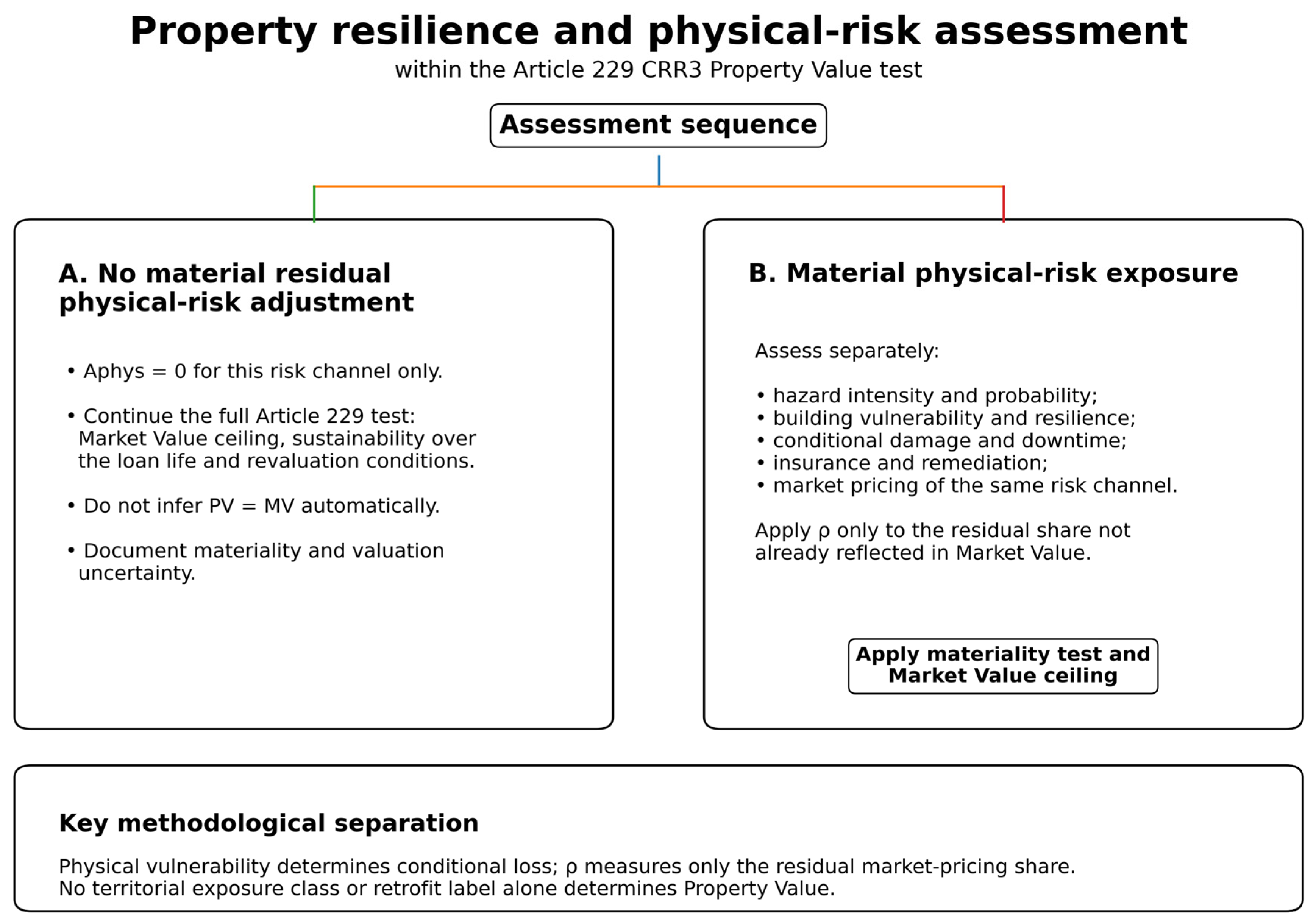
Figure 1 therefore presents a continuous residual-risk assessment rather than a binary exposed/not-exposed rule.
3.3. The Aphys Formula for Physical-Risk Adjustments
For event-based physical risks, this paper proposes the following first-order analytical formulation. It is designed to make the economic components of a possible residual adjustment explicit and auditable; it is not a complete probabilistic catastrophe-loss model, and it is not prescribed by CRR3, EBA or the ECB:
where:
Aphys = present value of the expected residual property-level loss attributable to physical, climate-related and environmental risks not incorporated into market value;
Pr(e,t) = probability of event e in period t under the selected hazard information and, where relevant, the selected forward-looking scenario; event intensity and asset vulnerability should be reflected in the conditional loss estimate or an underlying vulnerability function;
Physical vulnerability is conceptually upstream of the residual-pricing coefficient. For each event, the conditional damage component may be represented schematically as D(e,t) = f[I(e,t), Vbuilding, Rbuilding], where I(e,t) denotes event intensity, Vbuilding physical vulnerability, and Rbuilding resilience or mitigation. A retrofit or physical improvement should therefore affect Vbuilding/Rbuilding and the resulting conditional damage, downtime, or remediation assumptions. It should change ρ only where separate market evidence also demonstrates that the proportion of the remaining economic effect already incorporated in market value has changed.
Dunins(e,t) = physical damage to the property conditional on event e, measured through structural and non-structural repair/replacement costs required to restore damaged components, net of insurance recoveries that can reasonably be relied upon after deductibles, limits and exclusions, and excluding every item separately included in Crem;
Luse(e,t) = property-level economic loss from temporary unavailability, reduced habitability, lost rent or impaired use; borrower operating losses unrelated to the property’s own value are excluded;
Crem(e,t) = incremental post-event remediation or ancillary restoration cost not already included in Dunins, such as debris removal, temporary protection, environmental remediation or separately evidenced regulatory upgrading. Planned ex-ante adaptation expenditure is not probability-weighted as a contingent loss and should instead be treated separately as capex or another explicit adjustment where material and not already reflected in MV;
For each event-time pair, the economic content of Dunins and Crem must be mutually exclusive: Dunins(e,t) ∩ Crem(e,t) = ∅. The valuation file should reconcile the two buckets line by line. Repair or reinstatement of damaged structural and non-structural components belongs to Dunins; only ancillary or incremental post-event items not embedded in those repair estimates belong to Crem. This is an economic, not merely terminological, separation.
rp = discount rate used for expected residual losses, specified consistently on a nominal or real basis with the underlying loss estimates. It must not embed a risk premium for a risk already captured in event probabilities or expected losses;
m = total number of physical, climate-related and environmental event types considered for the purpose of the analysis;
n = loan term (or prudential analysis horizon).
The coefficient ρ(e,t), with 0 ≤ ρ(e,t) ≤ 1, represents the share of the relevant economic risk that remains unpriced in market value. It must not be selected at discretion. The proposed estimation hierarchy is: (i) define risk-homogeneous comparables by location, hazard, building type, vulnerability/resilience and relevant insurance characteristics; (ii) test whether transaction prices, rents, capitalization rates or other market evidence already reflect the risk, using matched-sales, repeat-sales, hedonic/spatial methods or other empirically appropriate designs where data permit; (iii) set ρ = 0 only where the relevant risk is demonstrably fully reflected, estimate 0 < ρ < 1 only where evidence supports partial pricing, and use ρ = 1 only where credible evidence supports the conclusion that the component is unpriced; and (iv) where evidence is insufficient, do not infer an arbitrary point estimate—report the data limitation and test a documented range in sensitivity analysis. This procedure makes ρ an empirically calibratable parameter rather than a free haircut coefficient. When partial pricing is evidenced, and the market-implied effect and the economic-loss benchmark can be expressed on the same present-value basis, an operational mapping may be written as ρ = max{0, min [1, 1 − Mpriced/Ggross]}, where Mpriced is the capitalized market effect attributable to the same risk channel, and Ggross is the present value of the corresponding gross expected property-level economic loss before the residual-pricing adjustment. Mpriced may be estimated from matched sales, hedonic/spatial coefficients, repeat-sales evidence, rent or capitalization-rate differentials, or evidence from a sufficiently comparable market, after controlling relevant confounders. The numerator and denominator must refer to the same hazard, property characteristics, time horizon, and economic-loss channel. Where either quantity is estimated as an interval, ρ should likewise be reported as a range; weak or non-comparable evidence should not be converted into a point estimate. This mapping is a proposed operational aid, not an empirically calibrated universal formula.
The Aphys formulation is primarily suited to event-based environmental, acute physical risks and geophysical events that can be represented through event probability and conditional loss. Chronic climate risks—such as gradual sea-level rise, chronic heat, drought or water scarcity—should not be forced into a single-event probability where that representation is inappropriate. Their value effects should instead be modeled through scenario-consistent changes in cash flows, operating costs, marketability, terminal value, or other empirically supported channels. Where multiple hazards overlap or are correlated, joint or conditional probabilities and vulnerability functions should be used where material; simple additivity is defensible only after overlap and repeated-loss effects have been controlled.
The formulation is designed to make the economic drivers of any prudential adjustment explicit and verifiable. It does not imply that every physical exposure should lead to a deduction from market value: an adjustment is justified only where the risk is materially relevant to the sustainability of value and is not already adequately incorporated into current prices.
The Aphys formulation may be informed by granular forward-looking hazard data and vulnerability functions linking event intensity to asset-specific damage. Its simplifying assumptions—including additivity, treatment of hazard dependence, insurance reliability, vulnerability, downtime and discounting—must be stated for each application. Results should be subjected to sensitivity analysis over the principal uncertain inputs, including ρ, event probabilities or scenario paths, vulnerability/damage assumptions, insurance recoveries, downtime and rp. The formulation remains a methodological proposal by the author and requires empirical calibration and external validation; it must not be interpreted as a source of standardized haircuts.
For example, at the European level, for the purpose of a simplified and more standardized screening of seismic damage, the European Macroseismic Scale 1998 (EMS-98) [
31] may also be used. It is the first intensity scale accompanied by illustrations, in which the drawings and photographic examples in
Section 5 facilitate field comparison with actually damaged structures. For damage classification, the scale distinguishes masonry and reinforced-concrete buildings and five grades (D1–D5), from negligible/slight damage to destruction; its use does not replace engineering analyses of hazard, vulnerability and fragility where required.
Although A
phys is labeled as an environmental and physical-risk adjustment, reflecting its primary purpose of quantifying residual physical-risk losses, its additive structure across event types and time periods is modular and can accommodate multiple hazards as well as additional measurable property-level loss channels. Social or Governance variables should not, however, be collapsed mechanically into A
phys. They may affect A
phys only where there is a documented causal link to one of its physical-risk inputs—for example by modifying vulnerability, property-level loss of use, remediation or compliance costs, insurance effectiveness, or another measurable consequence of a physical event. Otherwise, their value effects should be reflected separately through market evidence, cash flows, capex/opex, liquidity, legal/compliance costs or another expressly identified adjustment. This preserves the breadth of the ESG assessment recognized by the Italian Property Valuation Standard while maintaining analytical transparency and avoiding double counting [
5].
Where scenario analysis is used for non-stationary climate risks, the selected pathway, time horizon, downscaling source, and treatment of model uncertainty should be documented. In line with the EBA Guidelines, scenario analysis informs the inputs to the valuation framework; it does not translate supervisory climate scenarios into automatic property haircuts [
32].
Table 2 sets out the evidence chain expected in a real application. The numerical values used in Cases A-C remain constructed scenario assumptions; the table specifies how each input would instead be sourced, estimated, expressed, assigned an uncertainty range, and subjected to appropriate professional responsibility and control in an empirical valuation. The indication of the professional roles involved is, in any event, illustrative, since it must necessarily be aligned, and where necessary redefined, with the professional regulatory frameworks applicable in the different jurisdictions.
Table 2 summarizes the principal Aphys inputs, the supporting empirical evidence, and the controls adopted to avoid double counting.
3.4. Estimating PV for Income-Producing Properties
For income-producing properties, MV
RA may be represented by discounting property-level cash flows after distinct and non-overlapping physical-risk adjustments:
where:
NOIt is the expected net operating income in period t, based on market-supported and prudently normalized assumptions and excluding unsupported expectations of future price or rent increases;
ELt is the expected loss from physical damage and/or interruption of use;
Capext comprises planned adaptation or protection expenditure attributable to the property and not already reflected in MV or another cash-flow item;
ExtraOpext comprises additional insurance and maintenance costs;
r is the market discount rate, used on a nominal or real basis consistently with the cash flows;
Δr is an additional premium only for residual risk components not already incorporated in ELt, Capext, ExtraOpext, terminal value or the base market discount rate;
is the risk-adjusted terminal value at the end of the prudential analysis horizon. Continuing physical risk must be reflected through one, and only one, non-overlapping channel—for example, a risk-adjusted terminal NOI, a separately supported exit capitalization rate, or expected post-horizon capex/opex. It must not disappear mechanically after year n, and the chosen channel must be reconciled with ELt, Capext, ExtraOpext and Δr. The terminal assumptions must remain market-supportable and must not introduce speculative appreciation excluded by Article 229; assumptions on rent growth, inflation and exit capitalization should be internally consistent and should normalize rather than extrapolate short-term market-cycle peaks.
n = loan term (or prudential analysis horizon).
To avoid double counting, the preferred allocation is to reflect a quantifiable risk through the cash-flow item to which it directly relates; Δr should be used only for a distinct residual risk not captured elsewhere. ELt, Capext, ExtraOpext, Δr and must therefore be reconciled explicitly. Inflation, taxation and other model conventions must be applied consistently with the chosen nominal/real basis. The parameterization will differ across office, retail, industrial, logistics and other sectors because lease structures, insurance, market liquidity and vulnerability channels differ; coefficients should not be transferred across sectors without validation.
A capitalization rate k and a discount rate r are conceptually distinct. A capitalization rate converts a stabilized one-period income into value and embeds assumptions regarding growth, depreciation and risk; a discount rate prices multi-period cash flows. The same numerical value should therefore be used only where an explicit cash-flow convention makes them consistent—for example, a zero-growth level-perpetuity illustration with otherwise aligned assumptions. In empirical applications, k and r should be estimated and justified separately unless such a convention is demonstrated.
3.5. Estimating PV for Residential (Non-Income-Producing) Properties
For non-income-producing residential properties, the notation is standardized as follows: PV
R is the lower of current residential market value (MV
R) and the residential risk-adjusted analytical value (MV
RA,R), subject, on revaluation, to the additional Article 229(1)(e) ceiling:
The residential risk-adjusted market value (MV
RA,R) is obtained as follows:
where:
Aenergy = residual value effect attributable to energy performance only where it is material and not already reflected in MVR;
Alegal,residual = any remediable legal/planning/cadastral cost not already reflected in MVR. This is a baseline property/legal valuation issue, not an ESG category (Alegal (building, planning and cadastral compliance) is intended to identify non-compliances which, where remediable, would entail regularization costs or costs to restore the property to its compliant condition).
Aliquidity = residual marketability effect in a high-risk context only where it is empirically supported and not already incorporated into comparable prices. Planned ex-ante adaptation expenditure, where relevant, is treated separately rather than probability weighted as contingent loss.
The Aenergy, Alegal,residual and Aliquidity components are analytical variables of this framework, not adjustment categories prescribed by CRR3. Each is used only where the effect is material, adequately evidenced, and not already incorporated into market value. In a strictly subtractive residential implementation, the min operator is mathematically redundant whenever MVRA,R can only be below MVR; it is retained in Equation (5) to make the Article 229 market value ceiling explicit and to keep notation aligned with the general framework.
3.6. Avoiding Double Counting
A methodologically critical issue is the risk of double counting. If the comparables used to estimate MV are homogeneous with respect to the subject property’s material risks and those risks are already reflected in market prices, automatically applying an additional haircut would result in an unjustified penalty. The Aphys adjustment should therefore address only: (i) residual risk not incorporated into current prices; and/or (ii) reasonably foreseeable future conditions over the life of the loan that are materially relevant but not yet priced by the market. Article 229 CRR3 establishes the prudential outcome to be achieved but does not prescribe a specific haircut formula; the distinction between generic approaches and more granular, forward-looking methodologies instead emerges from the supervisory practices described by the ECB.
Where the comparables used to estimate MV have a demonstrably homogeneous risk profile, observed prices may already incorporate all or part of the relevant risk discount; materially different risk profiles require comparability adjustments. The identification procedure should therefore document: the hazard and property characteristics used to define the comparable set; whether price, rent or capitalization-rate evidence shows full, partial or no pricing; the empirical method used to infer any residual share; and the resulting ρ range. This procedure is intended to make the no-double-counting conclusion replicable rather than dependent on an unsupported expert assertion.
Because Article 229 does not define a universal numerical threshold for ‘significantly above’, materiality is operationalized in Equation (1) as a decision gate rather than as an automatic haircut. ΔV = MV − MVRA is compared with a documented mandate- or institution-specific criterion τ and with credible valuation/model uncertainty. If ΔV ≤ τ, or the difference lies within documented valuation uncertainty, PV remains MV under the proposed operational rule. Only where ΔV > τ and the difference also exceeds the documented uncertainty allowance (or lies outside the corresponding uncertainty range) does the lower-of-MV-and-MVRA rule apply. τ may be expressed as an absolute amount, a percentage of MV, or another documented metric, provided that it is translated onto a basis comparable with ΔV; neither τ nor the uncertainty allowance U is a CRR3-prescribed threshold.
3.7. Illustrative Numerical Cases and Sensitivity Analysis
The following cases operationalize the framework using transparent illustrative inputs. Their purpose is to show how the residual-risk logic, no-double-counting rule, and Aphys formulation work in practice across different property types and hazards. The comparable data and residual-risk shares are scenario inputs constructed for the worked applications; they are not presented as an observed empirical sample. Accordingly, the cases provide an internal-consistency and computational-implementation illustration, while empirical calibration and external validation remain necessary.
3.7.1. Case A—Residential Property in a Hydraulic-Hazard Area (Emilia-Romagna)
Asset and context. The subject is an 85 m2 ground-floor apartment in a 1980s residential building in Emilia-Romagna. It is assumed to have no dedicated hydraulic-mitigation measures and to be located in an area classified as P2 in the competent hydraulic-hazard mapping. The loan horizon is 25 years. The EPC is class E, and no material planning or cadastral non-compliance is assumed. The P2 administrative/hazard class is not converted mechanically into an annual damage probability; the event probability used below is a separate scenario input.
Market value and priced location risk. MV
R is estimated using the market comparison approach using three illustrative comparables. Two are in the same P2 micro-area and therefore provide evidence of the broad location-risk component already reflected in local prices; a third comparable outside the risk area is adjusted to the subject micro-area. The implied 17% location adjustment is constructed within the case and is not a generalizable empirical flood discount. Because the market value analysis already controls location risk and EPC characteristics, the base case does not apply a separate A
liquidity or A
energy deduction: absent additional evidence, doing so would risk double counting.
Table 3 presents the market comparison approach (MCA) and the resulting market value (MV) estimate for Case A.
Residual physical-risk adjustment. For the worked scenario, Prflood = 2.0% per year is assumed independently of the P2 label. Conditional property-level loss is EUR 18,000 of uninsured repair/replacement of damaged building components + EUR 3960 of property-level loss of use + EUR 8000 of ancillary post-event remediation (debris removal, drying/clean-up and temporary protection assumed in the scenario and excluded from the EUR 18,000 repair estimate) = EUR 29,960. The ground-floor position and absence of hydraulic mitigation affect the conditional-loss assumptions; independently, ρ = 40% is used as a residual market-pricing scenario assumption to represent partial market recognition of the same economic risk channel. It is not an empirical estimate and is varied separately in sensitivity analysis.
Sensitivity. The table varies event probability, residual-risk share, and the discount rate. The direction of the results is consistent with the framework: higher event probability or a larger residual unpriced share reduces PV, while a higher discount rate reduces the present value of a fixed expected-loss stream. The resulting MV
RA,R remains an analytical intermediate; in the base-case decision example in
Table 4, it becomes PV because ΔV exceeds both the illustrative τ and the uncertainty allowance. Sensitivity outputs remain conditional unless the same documented materiality test is applied to each scenario.
Table 4 presents the residual expected loss and the resulting property value for Case A.
Table 5 presents the sensitivity analysis for Case A.
3.7.2. Case B—Income-Producing Commercial Property in a High-Seismic-Hazard Area (Marche)
Asset and context. The subject is a 1200 m2 office/commercial building constructed in 1990 in a Marche municipality classified in Seismic Zone 1. The administrative zone signals high hazard but does not by itself determine site-specific seismic action or building damage probability; a real application would combine INGV/technical hazard inputs with the building vulnerability model. The worked case assumes an illustrative vulnerability/risk class D, no complete structural retrofit, no earthquake insurance, a 15-year loan, annual gross rent of EUR 96,000, 5% vacancy, and EUR 18,000 annual operating costs, giving a current NOI of EUR 73,200.
Market value. A market capitalization rate of 7.5% is assumed for comparable office properties in the same area. Because that market rate is derived from the same location, the broad seismic-zone component is treated as already priced. MV = 73,200/0.075 = EUR 976,000 (rounded).
Residual-risk and cash-flow architecture. The worked scenario assumes a 2.0% annual probability of an event capable of producing material structural damage. Physical vulnerability is represented through the assumed conditional-loss vector, not through ρ. The scenario uses ρ = 60% solely as a residual market-pricing assumption: it represents the share of the resulting property-level economic effects assumed not to be incorporated in the market evidence underlying MV. Neither Pr
seismic nor ρ is inferred mechanically from Seismic Zone 1 or from retrofit status. Conditional loss is kept mutually exclusive across components: EUR 350,000 represents uninsured structural/non-structural repair and replacement; EUR 45,000 represents 180 days of effective rental-income loss after the stated 5% vacancy allowance [EUR 96,000 × (1 − 0.05) × 180/365, rounded]; and EUR 80,000 represents ancillary post-event remediation and temporary-protection items assumed not to be included in the EUR 350,000 repair estimate. The scenario assumes no earthquake insurance, no rent recovery under the lease during unusability, and no reduction of the baseline operating costs during downtime; if recoverable or avoidable operating costs, insurance proceeds, or different lease obligations applied, L
use and/or the other cash-flow inputs would need to be adjusted accordingly. No additional Δr is included in the base case because there is no separate empirical evidence for a residual investor-risk premium beyond the quantified cash-flow loss; Δr should be used only for a distinct, non-overlapping residual component. As shown in
Table 6, Case B presents the expected residual property-level loss.
Capitalization and discounting convention.
The 7.5% market capitalization rate k is first used to derive MV from current stabilized NOI. A capitalization rate and a discount rate are conceptually distinct. For this constructed illustration only, the numerical discount rate r is also set at 7.5% under an explicit zero-growth, level-income/level-expected-loss convention, so that k = r when g = 0. The annual expected residual property level loss is EUR 5700. Continuing risk is not allowed to disappear after year 15: the terminal value is calculated from a risk-adjusted terminal NOI of EUR 73,200 − EUR 5700 = EUR 67,500, using the same 7.5% exit capitalization rate and no additional overlapping risk premium. Under these assumptions, the 15-year DCF plus risk-adjusted terminal value is equivalent to capitalizing the level risk-adjusted NOI, giving MVRA ≈ EUR 900,000 and a continuing residual adjustment of EUR 76,000. In an actual valuation, k and r would be estimated separately unless the same convention is empirically justified, and the terminal-risk channel would be documented explicitly.
Table 7 reports the property value determination for Case B.
Table 8 presents the sensitivity analysis for Case B.
The sensitivity analysis varies the residual market-pricing assumption (ρ) and physical-vulnerability/conditional-loss assumptions separately. An illustrative post-retrofit effect is represented through a lower conditional loss with ρ held constant unless independent market evidence supports a change in the proportion of risk already priced. A separate discount-rate or residual premium change would likewise require distinct evidence and must not duplicate expected losses or terminal-value assumptions.
In this respect, the treatment of terminal value deserves specific attention in a prudential DCF framework. D’Amato and Bambagioni [
33] discuss alternative approaches to the determination of exit value and emphasize the need to relate terminal-value assumptions to market conditions and to the long-term sustainability of cash flows.
More broadly, recent U.S. professional valuation literature supports a market-informed treatment of physical risk. Robinson [
34] argues that physical weather risk may be relevant to valuation where it is financially material and evidenced in market behavior, with potential transmission through operating and insurance costs, net operating income, capitalization and discount rates, resilience-related capital expenditure, liquidity and marketability. Importantly, the existence of physical exposure does not by itself justify a uniform adjustment; the valuation response should depend on whether and how market participants incorporate the relevant risk into pricing and investment decisions. This is consistent with the separation adopted here between physical vulnerability, market pricing and residual unpriced risk.
3.7.3. Case C—Residential Property with Partial Seismic Improvement (Messina, Sicily)
Asset and context. The subject is a 95 m2 second-floor apartment in a 1960s residential building in Messina, a municipality classified in Seismic Zone 1. The building is assumed to have undergone a partial seismic improvement in 2015, represented for the worked case by an illustrative class C vulnerability/risk profile compared with an unretrofitted class E profile. The loan horizon is 20 years, the EPC is D, no material planning or cadastral non-compliance is assumed, and hydrogeological risk in the micro-area is treated as immaterial. The administrative seismic zone is used for screening only; the scenario event probability is not inferred mechanically from the zone classification.
Market value and resilience pricing. Three illustrative comparables are used to isolate a resilience differential. Comp. 1 is aligned with the subject’s partial seismic improvement; Comp. 2 requires floor, condition, and EPC adjustments; Comp. 3 has otherwise similar characteristics but an unretrofitted class E profile and is adjusted upward to the subject’s class C profile. The 9.8% differential between Comp. 1 and Comp. 3 is an internal feature of the constructed case dataset, not an empirical estimate for the Messina market. It is used to demonstrate how resilience that is already priced in market value must not be deducted again through A
phys. The market comparison approach and the related resilience adjustment for Case C are reported in
Table 9.
Residual physical-risk adjustment. The worked scenario assumes Pr
seismic = 2.2% per year for an event capable of producing material building damage. The physical effect of the partial improvement is represented in the conditional-loss assumptions and in the resilience adjustment used in the comparable analysis; it is not used to determine ρ. Independently, ρ = 35% is adopted as a residual market-pricing scenario assumption representing partial pricing of the same economic risk channel. Neither Pr
seismic nor ρ is derived mechanically from the administrative zone or retrofit status. Conditional loss comprises EUR 95,000 of uninsured repair/replacement of damaged building components, EUR 3045 of property-level loss of use, and EUR 30,000 of ancillary post-event remediation/temporary-protection costs that are assumed not to be embedded in the EUR 95,000 repair estimate.
Table 10 presents the residual expected loss and the resulting property value for Case C.
As in Case A, no separate A
energy or A
liquidity is deducted in the base case because the comparable analysis already controls EPC and the local risk context. A further deduction would require separate evidence of a residual value effect not already reflected in market value. In the sensitivity analysis, the effect of a fuller retrofit is therefore represented by a lower conditional-loss assumption while ρ is held at 35%; ρ changes only in the separate market-pricing sensitivity.
Table 11 presents the sensitivity analysis for Case C.
3.7.4. Cross-Case Comparison
The three applications generate different analytical adjustments because the property type, physical vulnerability/conditional loss, residual unpriced-market share, horizon, and discounting assumptions differ. Physical vulnerability and ρ are varied separately. The results should not be read as market-wide haircut benchmarks or empirical building-performance estimates. Their role is to illustrate the computational behavior of the framework and to show explicitly how no-double-counting and materiality choices affect the result. A cross-case comparison of the base scenarios is presented in
Table 12.
Across the constructed base scenarios, the difference between MV and MVRA ranges from approximately 2.6% to 8.8%. These are outputs of the scenario assumptions, not empirically calibrated prudential ranges. In Case A, the 2.6% analytical difference is not treated as an automatic CRR3 deduction:
Table 4 provides a purely illustrative application of Equation (1), using τ = 2.0% of MV and an uncertainty allowance U = 1.5% of MV. Under those scenario assumptions, ΔV exceeds both MV and MV
RA,R becomes the illustrative PV; different documented mandate- or institution-specific criteria or uncertainty ranges could instead result in PV remaining equal to MV. For CRR purposes, the relevant effect must ultimately be assessed through the applicable ETV definition and exposure treatment rather than through the illustrative LTV ratios alone.