Physics-Generated Artificial Neural Network for Performance-Based Jet Grout Design in Soft to Medium Clays

Abstract

A jet grout design beneath raft foundations requires simultaneous selection of column geometry while satisfying bearing resistance and settlement criteria. This study develops a physics-generated artificial neural network (ANN) surrogate for performance-based screening of discrete jet grout configurations in soft to medium clays. Six engineering variables—undrained shear strength, constrained modulus, raft pressure, column diameter, spacing, and length—were used to generate 12,000 analytical cases representing 400 geometries. Equivalent ultimate column-grid pressure and settlement were calculated using established resistance formulations and an equal strain composite settlement model, respectively. Complete geometry groups were separated into training, validation, and independent test subsets to prevent information leakage, and a compact 6–24–12–2 ANN was trained to predict both responses simultaneously. For 2400 independent test cases representing 80 previously unseen geometries, the ANN achieved R² values exceeding 0.95 for both outputs and identified the same minimum-intensity feasible configuration as the analytical procedure in the illustrative design application. Independent three-dimensional finite-element simulations provided a complementary numerical assessment of representative settlement responses. The proposed framework integrates source-traceable analytical formulations, multi-output surrogate prediction, and performance constraints into a transparent preliminary design methodology for rapid screening of jet grout configurations. More broadly, it demonstrates how physics-generated machine learning surrogates can support the transition towards data-driven geotechnical design by systematically linking multidimensional engineering inputs with performance-based design decisions.

1. Introduction

Jet grouting is an in situ ground-improvement technique in which high-velocity fluid jets erode and mix the native soil with cementitious grout to form soilcrete columns or panels. The method is used for foundation strengthening, settlement reduction, excavation support, seepage control, and underpinning. However, the achieved column diameter, continuity, strength, and stiffness depend strongly on soil conditions, jetting parameters, grout properties, equipment configuration, and construction quality. Consequently, public agency guidance treats trial columns, coring, material testing, geometric verification, and performance testing as essential components of jet grout implementation rather than optional quality control measures [1,2].

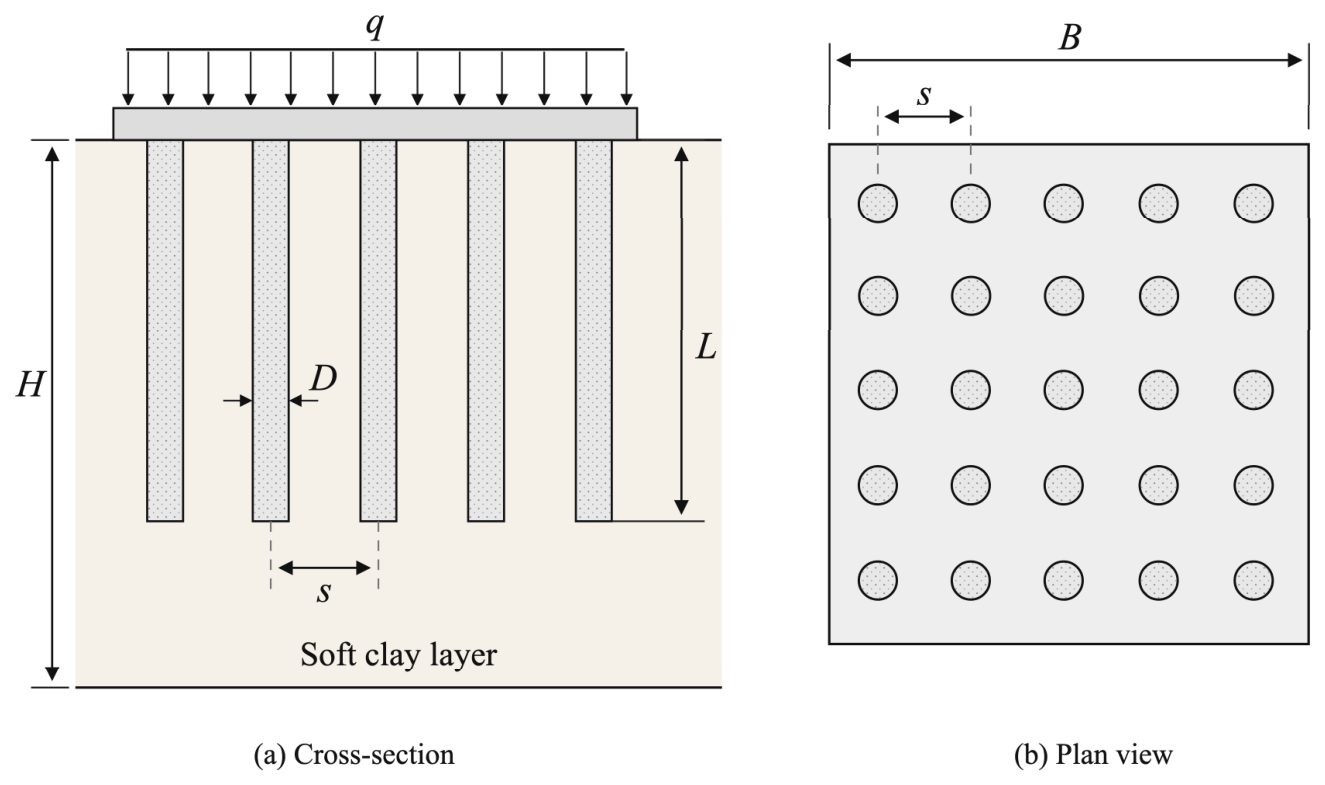
When jet grout columns are installed beneath a relatively rigid raft, the applied load is transferred to a composite ground system consisting of the stiffer soilcrete columns and the surrounding untreated soil. If the column tips do not penetrate into a competent bearing stratum, the columns behave as floating inclusions rather than end-bearing elements. Because of the stiffness contrast between soilcrete and a soft-to-medium clay, the columns generally attract a greater proportion of the applied stress, while the intervening soil continues to participate in load carrying and deformation. The resulting response therefore depends on column stiffness, area replacement ratio, length, spacing, interface mobilisation, and the compressibility of the untreated soil beneath and between the columns [3,4]. This composite behaviour means that a preliminary design procedure should not assess column resistance or settlement independently; both ultimate and serviceability requirements should be considered simultaneously.

Previous research has mainly focused either on predicting construction outcomes or on evaluating individual aspects of foundation response. Empirical and data-driven models have been proposed to predict the achieved diameter of single-, double-, and triple-fluid jet grout columns from ground and execution parameters [5,6]. Numerical studies have investigated various column diameters and centre-to-centre spacings, demonstrating that spacing and treatment length are important controls on foundation settlement [7]. These findings support the use of column diameter D, spacing s, and length L as the principal discrete geometry variables in a reduced preliminary design space. This limitation motivates the development of a computationally efficient surrogate capable of rapidly evaluating large numbers of candidate geometries while preserving consistency with the underlying analytical framework.

A jet grout design remains inherently affected by uncertainties associated with subsurface heterogeneity, construction variability, and the empirical or semi-empirical nature of many design relationships. Furthermore, post-installation verification is generally based on a limited number of core samples, material tests, or load tests, which cannot fully characterise the spatial variability of the treated ground. These uncertainties complicate the evaluation of numerous treatment alternatives while simultaneously satisfying ultimate and serviceability requirements [8,9]. In this context, surrogate machine learning models provide a practical means of learning multivariable input–output relationships and rapidly screening alternative treatment geometries within prescribed engineering constraints. Such models are particularly relevant when structured as scalable prediction components that can progressively incorporate analytical, numerical, laboratory, and field-derived response data as these become available. Accordingly, surrogate modelling can provide a useful bridge between conventional deterministic preliminary calculations and more data-informed performance-based jet grout designs.

Artificial intelligence and machine learning techniques have increasingly been applied to nonlinear geotechnical prediction problems, including soil-property estimation, foundation resistance, settlement, slope stability, and constitutive modelling [10]. Artificial neural networks are among the most frequently used approaches because they can approximate complex input–output relationships without requiring an explicitly prescribed functional form [11]. For example, machine learning models have been developed for pile-bearing-capacity prediction using measured soil, pile, and load-test data [8], while recent research on column-improved soft-to-medium clay has used numerical analysis databases and ANN models to predict settlement as a function of treatment geometry [4]. These studies confirm the potential of ANN-based surrogate models for rapid geotechnical response prediction. Nevertheless, most existing applications predict a single response quantity, such as bearing capacity, settlement, achieved diameter, or material strength, rather than directly identifying a feasible treatment geometry that satisfies multiple design criteria.

The reliability of a geotechnical ANN depends not only on its architecture but also on the physical relevance of the data generator, the selection of measurable input variables, and the independence of the validation procedure. Recent reviews have emphasised that the predictive performance of artificial intelligence models is strongly affected by dataset quality, input selection, evaluation strategy, and the extent to which physical knowledge is incorporated into the modelling framework [10,11]. Recent developments in structural engineering have further demonstrated the potential of integrating machine learning with mechanics- and physics-based modelling for efficient and generalizable engineering response prediction [12,13]. Recent studies have also extended machine learning applications from forward response prediction towards surrogate-assisted and inverse design frameworks, in which trained models are integrated with engineering constraints to support candidate evaluation and design-oriented decision-making [14,15]. Consequently, physically meaningful data generation and validation are equally important as network architecture in developing reliable engineering surrogate models.

The present study addresses these limitations through a source-audited, physics-generated ANN surrogate for performance-constrained jet grout geometry screening. Its contribution differs from studies that predict achieved column diameters or soilcrete strength from construction parameters. Here, the ANN is used to simultaneously estimate an equivalent column-grid resistance and total foundation settlement and is subsequently embedded in a discrete geometry selection procedure. Only six mechanically interpretable and practically obtainable variables are retained: undrained shear strength s_u, constrained modulus M_s, net raft pressure q, column diameter D, spacing s, and length L. The analytical equations, parameter intervals, and fixed assumptions are explicitly traceable to published technical sources. Moreover, complete D–s–L geometry groups, rather than individual database rows, are withheld during validation and independent testing. The resulting evaluation therefore examines interpolation to previously unseen geometries and reduces the risk of information leakage between the model-development and test datasets.

The ANN is not presented as a substitute for project-specific ground investigation, numerical analysis, trial-column construction, or field verification; rather, it is intended as a transparent preliminary screening surrogate for performance-based evaluation of candidate jet grout geometries. Although individual evaluations of the analytical equations are computationally inexpensive, the ANN provides a unified multi-output prediction engine that simultaneously maps soil, loading, and geometry variables to bearing resistance and settlement responses across the multidimensional design space and can be directly integrated with automated constraint-based geometry selection. Within this scope, the study aims to define a compact set of mechanically interpretable input variables; generate simultaneous bearing resistance and settlement targets using source-traceable analytical formulations; develop and assess the ANN through geometry-grouped training, validation, and independent testing; compare its predictions with the analytical data generator and a conventional regression baseline; and demonstrate a performance-constrained procedure for selecting feasible D–s–L configurations using bearing, settlement, and treatment-intensity criteria. In addition, complementary 3D FEM analyses are used to provide an independent numerical assessment of representative settlement responses obtained using the FHWA-based analytical calculation method. Importantly, the framework is structured so that the present analytical response generator can subsequently be replaced or recalibrated using higher-fidelity finite-element simulations, instrumented field trials, core-test results, or foundation load-test observations without modifying the downstream screening procedure. Accordingly, the principal motivation for the ANN lies in its role as the prediction component of a scalable surrogate-assisted design framework rather than in accelerating a single closed-form calculation.

2. Model Framework and Investigated Parameter Domains

2.1. Reference Foundation System and Soil Improvement Configuration

The reference problem consists of a 20 m × 20 m square rigid raft founded at the ground surface on a homogeneous, fully saturated, 20 m thick soft-to-medium clay layer. Jet grout columns are installed vertically beneath the raft in a regular square grid and are treated as floating inclusions because their tips remain within the compressible clay layer rather than penetrate into a competent bearing stratum. Under the rigid-raft assumption, the applied net foundation pressure is uniformly distributed at the raft level, while the stiffer soilcrete columns attract a greater share of the load than the surrounding untreated soil. This idealisation is consistent with the equal strain unit-cell concept commonly adopted in preliminary analyses of column-improved ground, in which column and soil deformations are represented through an equivalent composite response [3,4]. The model predicts the average vertical settlement of the raft and an equivalent ultimate resistance of the column grid for preliminary geometry screening. The square-grid arrangement is adopted because it provides a simple and reproducible relationship between column diameter, spacing, area replacement ratio, and tributary-cell area, while remaining representative of common design layouts used in column-supported foundations [3].

The reference system is intentionally simplified to isolate the effects of the six retained ANN inputs and to maintain full traceability between the analytical generator and the predicted outputs. The clay layer is therefore assumed to be homogeneous, isotropic, fully saturated, and characterised by constant values of undrained shear strength and constrained modulus within each generated case. The raft is assumed sufficiently rigid to suppress the differential flexural response, and the applied pressure is taken as vertical, concentric, and spatially uniform. The model does not explicitly simulate interface slip, progressive shaft mobilisation, local column bending, group interaction, or time-dependent excess-pore-pressure dissipation. These assumptions are appropriate for a transparent screening framework but should not be interpreted as substitutes for project-specific numerical modelling or field verification. Recent studies on jet grout column-improved soft to medium clays have similarly used idealised numerical or surrogate frameworks to isolate the effects of column spacing, length, and arrangement on settlement response [4]. Figure 1 illustrates the reference foundation geometry adopted in this study and defines the primary geometric parameters, including the column diameter (D), centre-to-centre spacing (s), column length (L), raft width (B), and thickness of the compressible clay layer (H).

2.2. ANN Input Variables and Evaluated Parameter Domains

The ANN input space comprises undrained shear strength (s_u), one-dimensional constrained modulus (M_s), net raft pressure (q), column diameter (D), centre-to-centre spacing (s), and column length (L). These variables were selected because they represent the principal soil-strength, compressibility, loading, and treatment-geometry mechanisms governing the response of a rigid raft supported by floating jet grout columns. Restricting the model to mechanically interpretable and practically obtainable parameters reduces unnecessary model complexity, improves transparency, and facilitates subsequent application to project-specific conditions. Undrained shear strength governs the short-term shaft and base resistance mobilised in the clay, whereas the constrained modulus controls vertical compression within the untreated and treated zones. Net raft pressure represents the foundation demand, while D, s, and L determine the column cross-sectional area, area replacement ratio, tributary-cell geometry, available shaft-resistance length, and thickness of the improved layer.

The parameter domains and sampling procedures used in this study are summarised in

Table 1. ANN input variables and source-audited parameter domains.

Input Variable	Adopted Domain	Sampling Strategy and Engineering Basis
Undrained shear strength, su	12–48 kPa	Latin hypercube sampling; represents soft-to-medium clay conditions [18].
Constrained modulus, Ms	0.60–2.00 MPa	Latin hypercube sampling; based on reported soft to medium clays [19].
Net raft pressure, q	50–250 kPa	Latin hypercube sampling; covers representative raft pressures [7,20].
Column diameter, D	0.60–1.00 m	Discrete 0.10 m increments; consistent with published jet grout geometries [1,2,7].
Column spacing, s	1.50–2.50 m	Discrete 0.25 m increments; covers commonly analysed grid spacings [7].
Column length, L	5–20 m	Discrete 1 m increments; represents partial to full treatment depth [1,2,7].

. The continuously varying variables s_u, M_s, and q are sampled using Latin hypercube sampling. This method stratifies the range of each variable and selects samples so that all portions of the prescribed domain are represented more uniformly than in simple random sampling. It therefore improves coverage of the multidimensional input space, reduces clustering and unrepresented intervals, and allows a broad range of soil and loading combinations to be explored with a comparatively limited number of cases [16]. In contrast, D, s, and L are treated as discrete variables because these parameters are selected in practice from constructible and operationally meaningful increments. This separation between continuously sampled site variables and discrete design variables also enables complete geometry groups to be withheld during validation and independent testing [17].

The specified intervals define the interpolation domain of the present ANN. Application to soil properties, loading levels, or column geometries outside these ranges requires regeneration of the physics-based database and retraining of the surrogate model. The constrained modulus interval of 0.60–2.00 MPa is specifically derived from the laboratory values reported for soft to medium clays in reference [19]. To avoid adding poorly constrained material inputs, q_u,jg is fixed at 2.0 MPa. FHWA reports typical soilcrete strengths in clays of 250–500 psi, approximately 1.72–3.45 MPa [1]. A screening modulus E_jg = 100q_u,jg = 200 MPa is used. The ratio is reported for the jet-mixed zone in the FHWA deep mixing manual; it is adopted here as a transparent, conservative screening assumption [3]. Project-specific core strength and stiffness should replace both fixed values. Although representative reference values of q_u,jg = 2.0 MPa and E_jg = 200 MPa were adopted as fixed parameters for the baseline dataset, these quantities are not inputs for the trained six-input ANN. Changing either value therefore requires regeneration of the corresponding analytical database or retraining of the present surrogate. Sensitivity evaluations indicate that, in deep soft-to-medium clay deposits, overall foundation performance and settlement reduction are primarily governed by the area replacement ratio and soil–column interface mobilisation rather than moderate variations in soilcrete stiffness [4,7,17]. Nevertheless, in future extensions, q_u,jg and E_jg may be incorporated as additional continuous ANN inputs so as to represent project-specific soilcrete properties directly within the surrogate framework, thereby accommodating different jet-grouting technologies and binder formulations.

3. Physics-Generated Bearing and Settlement Targets

Establishing reliable bearing capacity and settlement targets for the analytical dataset requires a precise formulation of the spatial configuration and the composite mechanical properties of the treated zone [20,21]. For columns installed on a square grid, the cross-sectional area of an individual column (Ac) and the corresponding area replacement ratio (a_r) are defined in Equation (1) and Equation (2), respectively:

$$A_c={\displaystyle \frac{\pi D^2}{4}}$$

(1)

$$a_r=A_c/s^2={\displaystyle \frac{\pi D^2}{4s^2}}$$

(2)

where D is the column diameter, and s is the centre-to-centre spacing. The area replacement ratio links the discrete column geometry to the stiffness of the treated ground and represents the fraction of each square tributary cell occupied by soilcrete.

Under the equal strain idealisation, the soilcrete column and surrounding clay within the treated zone are assumed to undergo the same average vertical strain. The equivalent constrained modulus of the treated zone (M_comp) is therefore calculated as given in Equation (3):

$$M_{comp}=a_s{E}_{jg}+\left(1-a_s\right)M_s$$

(3)

where E_jg is the assigned soilcrete modulus, and M_s is the constrained modulus of the untreated clay. Equation (3) follows the composite modulus formulation presented in the FHWA design guidance for preliminary settlement assessment [3]. The expression provides a transparent first-order representation of the effects of column stiffness and the area replacement ratio but does not explicitly simulate interface slip, progressive column mobilisation, local stress redistribution, or three-dimensional group interaction. FHWA similarly presents the composite modulus approach within an equal strain settlement framework and indicates that compression beneath the treated zone should be assessed separately.

Previous studies have shown that equivalent composite stiffnesses may differ from the effective stiffness mobilised at the field scale because of group interactions and construction-related factors [22]. Accordingly, Equation (3) forms the basis of the physics-generated training database used for ANN development. Because the same mechanically consistent formulation is applied to every geometry and soil condition, the resulting database provides a transparent, reproducible, and internally consistent representation of the stiffness contribution of the treated zone.

3.1. Settlement Target

The settlement target is calculated as the sum of the compression within the treated zone and the compression of the untreated clay beneath the column tips. Within the treated zone, the equal strain assumption implies that the soilcrete columns and surrounding clay undergo the same average vertical shortening. The corresponding compression is calculated using the equivalent composite modulus, as given by Equation (4):

$$S_1={\displaystyle \frac{qL}{M_{comp}}}$$

(4)

where q is the uniform net raft pressure, and L is the column length. Equation (4) represents the average one-dimensional compression S₁ of the improved layer and is consistent with the FHWA composite modulus approach, in which treated-zone settlement is obtained by dividing the applied stress by the equivalent modulus and multiplying by the treatment thickness [3].

For floating columns with L < H, the compressible clay extending beneath the column tips contributes an additional settlement component. A 2:1 stress-spread approximation is adopted to represent the reduction in vertical stress with depth below the raft. For a square raft of width B, the vertical stress increment at depth z, measured from the raft level, is calculated using the approximation given by Equation (5):

$$\Delta \sigma \left(z\right)=q{\left({\displaystyle \frac{B}{B+z}}\right)}^2$$

(5)

Assuming a constant constrained modulus with depth, integration of the vertical strain Δσ(z)/Ms between the column tip level L and the base of the compressible layer H yields the settlement contribution given by Equations (6)–(8):

$$S_2={\displaystyle \frac{q{B}^2}{M_s}}\left({\displaystyle \frac{1}{B+L}}-{\displaystyle \frac{1}{B+H}}\right) \mathrm{f}\mathrm{o}\mathrm{r} \mathrm{L}<\mathrm{H}$$

(6)

$$S_2=0 \mathrm{f}\mathrm{o}\mathrm{r} \mathrm{L}=\mathrm{H}$$

(7)

$$S=S_1+S_2$$

(8)

The separation of treated-zone compression and sub-column compression is consistent with FHWA guidance, which permits the settlement of the underlying untreated ground beneath the jet grout column tips, represented here by S₂, to be estimated using a load-spread approach [3].

The resulting S value is an average, equivalent one-dimensional settlement index for comparing candidate geometries within the prescribed parameter space. It does not predict the rate of consolidation, excess-pore-pressure dissipation, differential raft settlement, soil anisotropy, stress-dependent stiffness, or installation-induced changes in the surrounding clay. The use of a constant M_s also assumes that the adopted modulus represents the relevant foundation stress range. These limitations are intentionally retained to preserve transparency in the initial analytical generator; subsequent versions should replace or calibrate the settlement labels using project-specific coupled-consolidation analyses or field observations.

3.2. Bearing Resistance Target

The geotechnical resistance of an individual jet grout column is evaluated as the combined contribution of shaft and base resistance. In the absence of a generally accepted shaft-resistance formulation specifically developed for floating jet grout columns in soft clay, the FHWA drilled shaft α-method is employed as a transparent and source-traceable analytical analogue for preliminary resistance assessment [22,23]. The adopted α-method should be regarded as a source-traceable analytical analogue for preliminary screening rather than a definitive representation of jet grout interface behaviour. Variations in mobilised adhesion directly affect the shaft-resistance component and may consequently modify the equivalent column-grid resistance and the set of geometries satisfying the prescribed bearing resistance criterion. Project-specific load-test data or calibrated interface resistance should therefore be used where available during detailed design. Accordingly, the adhesion factor, unit shaft resistance, and ultimate shaft resistance are calculated using Equations (9)–(11), respectively:

$$\alpha =0.30+{\displaystyle \frac{0.17}{s_u/p_a}}$$

(9)

$$f_s=\mathit{min}\left(\alpha s_u,\hspace{0.33em}{s}_u\right)$$

(10)

$$Q_{s,u}=\pi DL{f}_s$$

(11)

where pa = 100 kPa is the reference atmospheric pressure, and s_u is expressed in the same stress unit. The corresponding unit shaft resistance is f_s, and the ultimate shaft resistance of one column is Q_s,u. The base resistance is determined from Equation (12):

$$Q_{b,u}=N_c{s}_u{A}_c$$

(12)

where N_c is the clay base resistance factor. Following FHWA GEC 10 [20], N_c is assigned according to the undrained shear strength of the clay within the investigated parameter range.

The geotechnical resistance of the column and the material resistance of the soilcrete are subsequently calculated using Equations (13) and (14), respectively. The ultimate column resistance is then obtained as the lower of the geotechnical and material resistance limits according to Equation (15):

$$Q_{\mathrm{g}\mathrm{e}\mathrm{o},u}=Q_{s,u}+Q_{b,u}$$

(13)

$$Q_{\mathrm{m}\mathrm{a}\mathrm{t},n}=A_c{q}_{u,\mathrm{j}\mathrm{g}}$$

(14)

$$Q_{\mathrm{c}\mathrm{o}\mathrm{l},u}=\min \left(Q_{\mathrm{g}\mathrm{e}\mathrm{o},u},\hspace{0.33em}{Q}_{\mathrm{m}\mathrm{a}\mathrm{t},n}\right)$$

(15)

Finally, the equivalent ultimate column-grid pressure is obtained by dividing the ultimate column resistance by the tributary-cell area, as given by Equation (16). The corresponding bearing resistance ratio is subsequently calculated using Equation (17):

$$q_{\mathrm{u}\mathrm{l}\mathrm{t},\mathrm{e}\mathrm{q}}={\displaystyle \frac{Q_{\mathrm{c}\mathrm{o}\mathrm{l},u}}{s^2}}$$

(16)

$$F{S}_b={\displaystyle \frac{q_{ult,eq}}{q}}$$

(17)

The ANN is trained to predict q_ult,eq, whereas the required bearing resistance ratio is applied subsequently during geometry screening. This separation allows the same trained surrogate to be evaluated under different project-specific resistance requirements without retraining.

Equations (9)–(17) provide a transparent analytical framework for estimating the equivalent resistance of floating jet grout column grids during preliminary design. The formulation evaluates the resistance mobilised by the columns within their tributary grid areas while representing the governing shaft, base, and soilcrete material resistance mechanisms through source-traceable equations. Accordingly, q_ult,eq is interpreted as a conservative column-resistance-based equivalent grid capacity for preliminary performance screening, obtained by distributing the governing column resistance over the corresponding tributary-cell area. The surrounding untreated soil contributes to the composite deformation response through the settlement formulation, while its additional ultimate resistance is not superimposed on q_ult,eq. This provides a transparent and conservative resistance measure for comparing candidate jet grout geometries, while a more detailed assessment of the complete raft–column–soil system, including composite load transfer, column group interaction, and project-specific material behaviour, remains part of the subsequent project-specific design verification.

4. Development of the Artificial Neural Network

4.1. Database Generation

The database was constructed by combining five column-diameter levels, five spacing levels, and sixteen column-length levels, resulting in 5 × 5 × 16 = 400 discrete D-s-L geometries. For each geometry, 30 combinations of undrained shear strength su, constrained modulus M_s, and net raft pressure q were generated using three-dimensional Latin hypercube sampling. This procedure produced a total of 400 × 30 = 12,000 cases. Latin hypercube sampling was adopted because it distributes samples more uniformly across the prescribed multidimensional parameter space than simple random sampling, reduces clustering, and enables the continuous soil and loading domains to be represented efficiently with a limited number of cases [16]. The same number of samples was generated for every geometry so that no diameter–spacing–length configuration was overrepresented during ANN training.

Each database row contains the input vector x = [s_u, M_s, q, D, s, L] and the corresponding target vector y = [q_ult,eq, S]. The target values were generated directly from Equations (1)–(17) using the reproducible computational script. Because all outputs were generated deterministically from the analytical formulations, the database is free from measurement uncertainty and experimental variability. Accordingly, the ANN represents a computational surrogate of the underlying analytical framework, enabling rapid prediction of bearing resistance and settlement throughout the investigated design space.

4.2. Network Architecture and Training Procedure

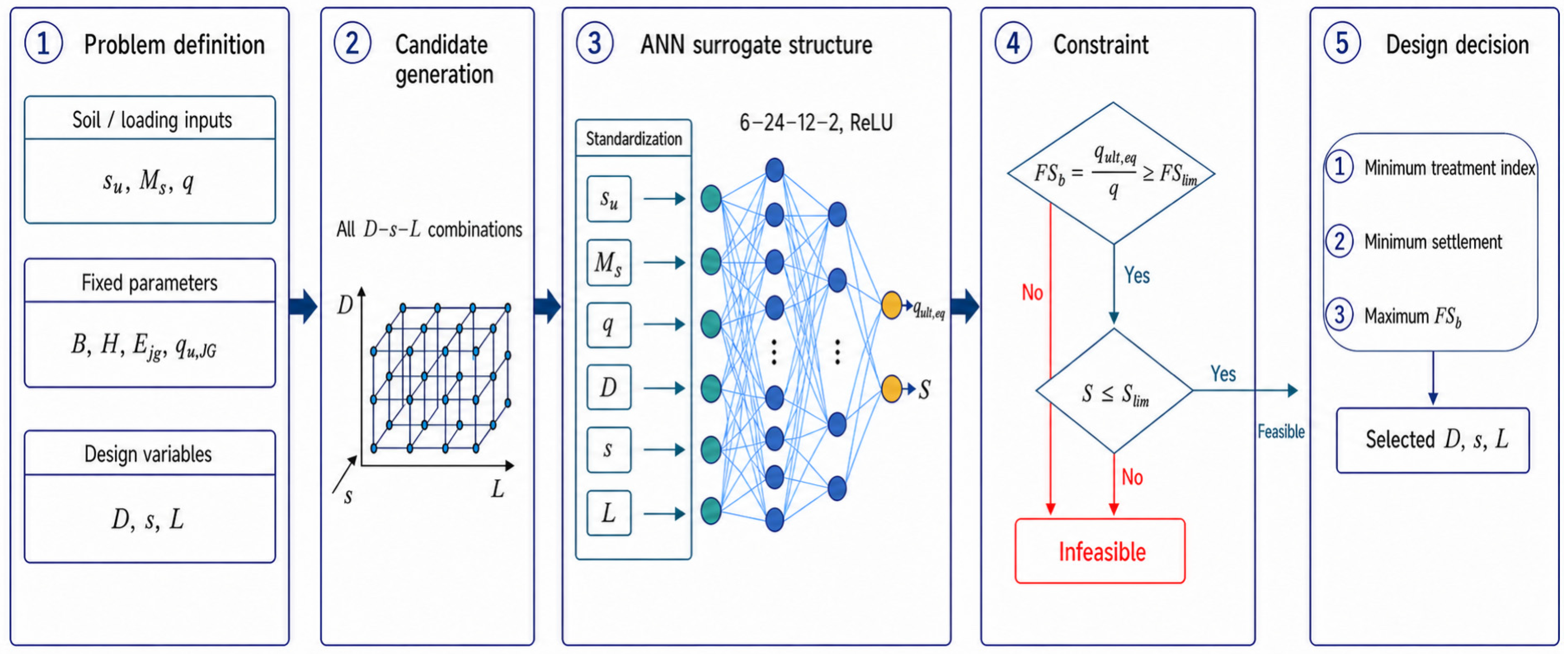
A fully connected feed-forward artificial neural network was developed to approximate the nonlinear mapping between the geotechnical, loading, and geometry inputs and the bearing resistance and settlement responses. The network consists of an input layer comprising the variables s_u, M_s, q, D, s, and L; two hidden layers containing 24 and 12 neurons, respectively; and an output layer with two neurons representing the equivalent ultimate column-grid pressure q_ult,eq and the total settlement S. Rectified linear unit (ReLU) activation functions are used in the hidden layers, whereas the output layer uses a linear activation function because both target variables represent continuous regression outputs. The adopted 6–24–12–2 network architecture is schematically illustrated in Figure 2.

All input variables and target values are standardised using the mean and standard deviation calculated exclusively from the training subset. The same training-derived transformation parameters are subsequently applied to the validation and independent test subsets. This procedure prevents information from the withheld geometries from influencing model fitting and avoids scaling-related data leakage. Predicted outputs are transformed back to their original units before the performance metrics are calculated.

The network is trained using the Adam optimisation algorithm [24], with an initial learning rate of 0.001 and a batch size of 256. Adam was adopted because it combines adaptive parameter-specific learning rates with momentum-based optimisation and is well suited to nonlinear regression problems involving input variables with different sensitivities. For the present six-input/two-output regression problem, a compact 6–24–12–2 feed-forward architecture was adopted. The purpose of the network selection was not to establish an optimised ANN topology, but to provide a parsimonious surrogate representation of the nonlinear analytical input–output relationships while avoiding unnecessary architectural complexity. The hidden layers use ReLU activation, while the output layer is linear for continuous regression. Early stopping used a 0.10 internal validation fraction from the training subset, with a minimum improvement of 10⁻⁷, a patience of 50 iterations, and a maximum of 1500 training iterations. The same settings were used during the hyperparameter assessment.

To establish a systematic basis for the selection of the ANN architecture and to assess the trade-off between predictive performance and model complexity, a structured hyperparameter analysis was conducted. Five hidden-layer architectures, (12, 6), (24, 12), (32, 16), (48, 24), and (32, 16, 8), were considered together with ReLU and tanh activation functions and batch sizes of 64, 128, and 256. The initial learning rate was held at 0.001, corresponding to that adopted in the main ANN model (

Table 2. Validation performance for the investigated ANN architecture–activation–batch-size combinations.

Hidden Layers	Activation	Batch Size	MSE	qult,eq R2/RMSE	S R2/RMSE
12–6	ReLU	64	0.005854	0.99491/10.99	0.99640/18.70
		128	0.005361	0.99550/10.33	0.99643/18.62
		256	0.004748	0.99652/9.09	0.99598/19.77
	tanh	64	0.001267	0.99880/5.35	0.99940/7.66
		128	0.001523	0.99859/5.78	0.99921/8.77
		256	0.002151	0.99776/7.30	0.99931/8.19
24–12	ReLU	64	0.001191	0.99914/4.53	0.99898/9.95
		128	0.001139	0.99909/4.65	0.99917/8.99
		256	0.001210	0.99919/4.38	0.99884/10.60
	tanh	64	0.000489	0.99950/3.44	0.99982/4.15
		128	0.000360	0.99962/3.01	0.99990/3.18
		256	0.000749	0.99921/4.34	0.99978/4.61
32–16	ReLU	64	0.000759	0.99942/3.71	0.99940/7.67
		128	0.000573	0.99953/3.33	0.99959/6.29
		256	0.000748	0.99934/3.97	0.99956/6.52
	tanh	64	0.000233	0.99978/2.30	0.99989/3.27
		128	0.000263	0.99976/2.39	0.99986/3.67
		256	0.000231	0.99977/2.31	0.99990/3.11
32–16–8	ReLU	64	0.000559	0.99960/3.09	0.99952/6.86
		128	0.000566	0.99957/3.21	0.99955/6.58
		256	0.000910	0.99935/3.94	0.99921/8.77
	tanh	64	0.000369	0.99969/2.70	0.99975/4.94
		128	0.000377	0.99967/2.80	0.99977/4.68
		256	0.000276	0.99977/2.33	0.99981/4.28
48–24	ReLU	64	0.000347	0.99972/2.56	0.99974/4.99
		128	0.000333	0.99975/2.42	0.99972/5.18
		256	0.000292	0.99980/2.17	0.99972/5.18
	tanh	64	0.000145	0.99986/1.80	0.99993/2.65
		128	0.000229	0.99979/2.23	0.99988/3.48
		256	0.000168	0.99984/1.95	0.99992/2.74

), so that the effects of network size, activation function, and batch size could be examined directly. This produced 30 architecture–activation–batch-size combinations. Adam optimisation and the same early stopping strategy were maintained for all configurations. Performance was compared using the 48 geometry-grouped validation geometries, while the 80 independent test geometries remained excluded from this sensitivity assessment.

As shown in Table 2, both ReLU- and tanh-based networks achieved high predictive accuracy across a broad range of architectures and batch sizes. Increasing network size generally reduced the validation error, whereas the influence of batch size was comparatively modest and configuration dependent. The lowest validation error in the focused comparison was obtained using the 48–24 tanh architecture with a batch size of 64. However, this larger architecture contains approximately 1562 trainable parameters, compared with only 494 parameters in the adopted 6–24–12–2 network. The adopted 24–12 ReLU configuration already achieved validation (R²) values of 0.9992 for q_ult,eq and 0.9988 for settlement. Consequently, the additional reduction in validation error obtained by increasing network complexity was not considered necessary for the intended screening-level application. The 6–24–12–2 architecture was therefore retained as a deliberately parsimonious surrogate that provides a favourable balance between predictive accuracy, model complexity, and transparency. The sensitivity analysis further demonstrates that the principal physics-generated input–output relationships are reproduced consistently by multiple ANN configurations rather than depending on a narrowly tuned network topology.

4.3. Geometry-Grouped Training, Validation, and Testing

A conventional random row split is unsuitable for the present database because each discrete D-s-L geometry is associated with multiple closely related su-Ms-q combinations. Consequently, randomly assigning individual rows to different subsets would distribute cases sharing the same geometry across both the training and testing datasets. As a result, the reported prediction accuracy would primarily reflect interpolation among soil and loading conditions for previously encountered geometries rather than the ability of the ANN to generalise to new design configurations.

To eliminate this source of information leakage, each discrete D-s-L configuration is assigned a unique geometry identifier. Complete geometry groups are then randomly allocated to the training, validation, or independent test subset, ensuring that every soil–loading combination associated with a withheld geometry remains completely unseen during model development. The final partition comprises 272 training geometries, 48 validation geometries, and 80 independent test geometries, corresponding to 68%, 12%, and 20% of the complete geometry space, respectively, as given in

Table 3. Training, validation, and test partition of the physics-generated database.

Subset	Geometries	Cases	Role
Training	272	8160	Estimation of network weights and scaling parameters
Validation	48	1440	Early stopping and model-development assessment on unseen geometries
Independent test	80	2400	Final evaluation on geometries not used during model development
Total	400	12,000	Complete physics-generated database

. This geometry-grouped partitioning provides a rigorous evaluation of the ANN by assessing its predictive capability on entirely unseen design configurations rather than on additional soil-property combinations associated with previously encountered geometries.

The independent test subset is reserved until the network architecture and training procedure have been established. Its results therefore assess the ability of the ANN to interpolate to diameter–spacing–length combinations that were not encountered during model fitting. Since the withheld geometries remain within the investigated ranges of D, s, and L, the independent test evaluates interpolation across previously unseen geometries within the audited design domain rather than extrapolation beyond it.

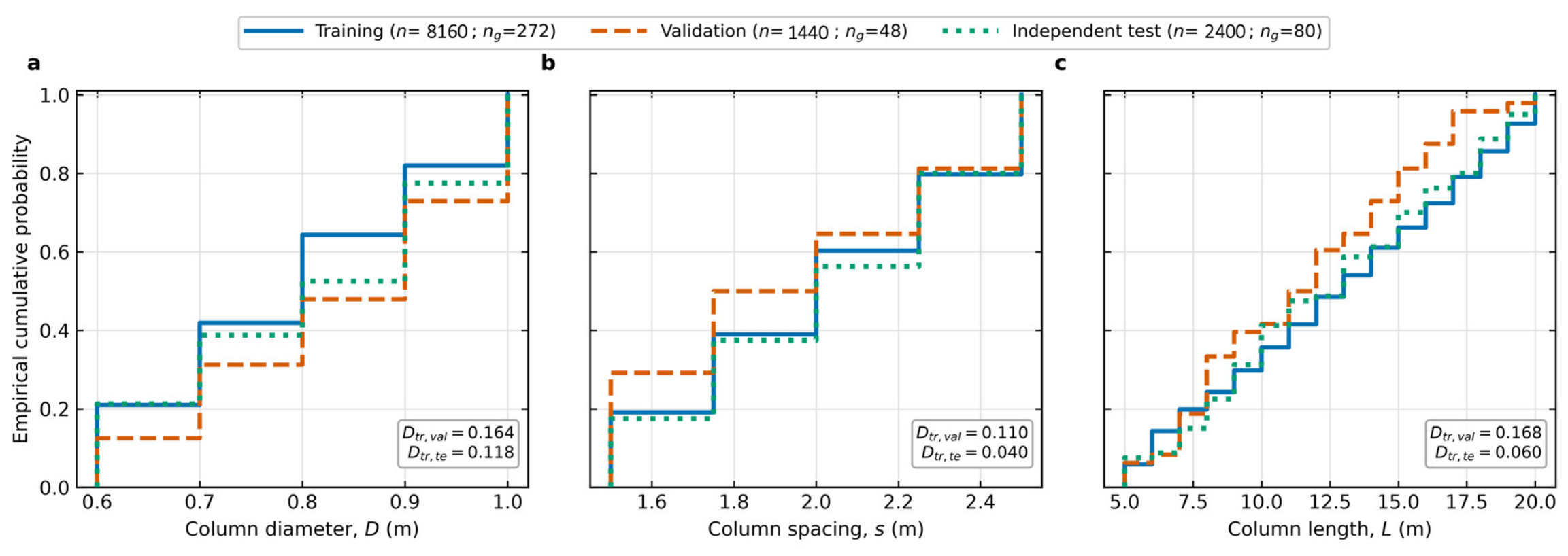
The empirical cumulative distribution functions of column diameter D, column spacing s, and column length L for the geometry-grouped training, validation, and independent test subsets are presented in Figure 3. Here, n is the number of individual samples and ng is the number of distinct geometric configurations. The statistics D_tr,val and D_tr,te quantify the maximum distributional differences between the training subset and the validation and independent test subsets, respectively. All samples associated with a given D-s-L configuration were assigned exclusively to one subset. This geometry-grouped partitioning preserves complete independence between model development and evaluation by ensuring that no design configuration is shared across different subsets. Consequently, the reported prediction performance reflects the generalisation capability of the ANN to previously unseen jet grout geometries rather than to additional soil-property combinations associated with previously encountered designs [25,26,27,28].

This partitioning strategy is consistent with previous findings showing that ignoring hierarchical or repeated-measure data structures during model validation can underestimate prediction errors and produce overly optimistic estimates of model performance [26,27].

Prediction performance was evaluated separately for q_ult,eq and S using the coefficient of determination R², root mean square error (RMSE), mean absolute error (MAE), and mean absolute percentage error (MAPE). Reporting both scale-dependent and dimensionless measures provides a more complete assessment than relying on R² alone. To establish whether the nonlinear ANN offers a meaningful improvement over a linear approximation, a multiple linear regression (MLR) model was developed using the same input variables together with the identical geometry-grouped training and independent test datasets.

Output-specific permutation sensitivity is evaluated using the independent test subset. Each standardised input is shuffled individually while the remaining inputs are retained in their original order, and the resulting increase in mean square error is calculated for each output. A greater error increase indicates that the ANN relies more strongly on the shuffled variable for the corresponding prediction [29]. These values describe the sensitivity of the trained surrogate within the adopted equations and parameter ranges; they should not be interpreted as universal geotechnical importance rankings.

In addition to the conventional regression performance metrics, agreement between the ANN predictions and analytical targets was evaluated using Bland–Altman analysis. Although R² quantifies the proportion of target variance reproduced by the model, it does not directly assess numerical agreement or systematic prediction bias. For each independent test observation, the paired difference (d_i) and the paired mean (m_i) were calculated according to Equations (18) and (19), respectively:

$$d_i=y_{i,\mathrm{A}\mathrm{N}\mathrm{N}}-y_{i,\mathrm{a}\mathrm{n}\mathrm{a}\mathrm{l}\mathrm{y}\mathrm{t}\mathrm{i}\mathrm{c}\mathrm{a}\mathrm{l}}$$

(18)

$$m_i={\displaystyle \frac{y_{i,\mathrm{A}\mathrm{N}\mathrm{N}}+y_{i,\mathrm{a}\mathrm{n}\mathrm{a}\mathrm{l}\mathrm{y}\mathrm{t}\mathrm{i}\mathrm{c}\mathrm{a}\mathrm{l}}}{2}}$$

(19)

The mean difference was interpreted as prediction bias, and the approximate 95% limits of agreement were calculated and given with the standard deviation of the paired differences. This analysis was used to identify systematic and magnitude-dependent prediction errors. The limits of agreement were interpreted as descriptive ANN–analytical error bounds rather than engineering acceptance limits. All calculations were performed on the geometry-grouped independent test subset, ensuring that no geometric configuration used for model development appeared in the final evaluation data [30,31].

The geometry-grouped holdout strategy ensures that the independent test set contains only D–s–L configurations that were not encountered during model training or validation. The predefined random seed was retained to ensure exact reproducibility of the data partition. Accordingly, the reported performance metrics quantify surrogate fidelity for this independent grouped test set within the prescribed analytical domain.

To evaluate the robustness of the surrogate with respect to the particular geometry-grouped data partition, the complete model-development procedure was additionally repeated using ten independently generated geometry-grouped partitions while retaining the adopted 6–24–12–2 ReLU architecture. This repeated grouped-splitting procedure provides an additional assessment of the sensitivity of the reported performance to the specific allocation of complete geometries among the model-development and test subsets. Across these repeated partitions, the mean independent test performance was R² = 0.99894 and RMSE = 3.96 kPa for q_ult,eq, and R² = 0.99917 and RMSE = 9.02 mm for settlement. As summarised in

Table 4. Robustness and LOEO assessment.

Test	R2, qult,eq	RMSE (kPa)	R2, S	RMSE (mm)
Original independent test	0.99890	4.01	0.99900	9.81
10 repeated geometry-grouped splits	0.99894 ± 3.2 × 10−4	3.96 ± 0.34	0.99917 ± 1.6 × 10−4	9.02 ± 0.73
Leave-one-D-level-out, mean	0.99528	6.52	0.99822	12.63
Leave-one-s-level-out, mean	0.98736	10.35	0.99885	10.55
Leave-one-L-level-out, mean	0.99776	4.63	0.99540	9.94

, the limited between-partition variability indicates that the reported predictive performance is stable with respect to the allocation of complete geometries and is not dependent on a single geometry-grouped partition.

Given the physics-generated and geometry-structured nature of the present database, the LOEO concept was implemented in a form directly aligned with the underlying design hierarchy, namely a leave-one-geometric-level-out assessment. In separate analyses, each complete level of column diameter D, spacing s, or column length L was excluded from model training and used exclusively for testing, resulting in 5 diameter-level, 5 spacing-level, and 16 length-level holdouts. The mean R² values for q_ult,eq were 0.99528, 0.98736, and 0.99776 when withholding D, s, and L, respectively, while the corresponding values for settlement were 0.99822, 0.99885, and 0.99540. The consistently high predictive performance obtained across all three groups of holdout analyses demonstrates that the surrogate retained its predictive capability even when complete geometric levels were entirely absent from model training. This provides a more stringent assessment of generalisation than interpolation among previously represented geometric levels and complements the geometry-grouped independent test procedure.

4.4. Performance-Based Geometry Selection

Following training, the ANN serves as the prediction engine within a discrete geometry screening procedure. For prescribed values of s_u, M_s, and q, the trained model predicts q_ult,eq and S for every candidate combination of D, s, and L contained in the audited geometry space [32,33]. A candidate geometry is classified as feasible when it simultaneously satisfies the required bearing resistance ratio and the allowable settlement condition:

$${\displaystyle \frac{q_{ult,eq}}{q}}\ge F{S}_{req}$$

(20)

$$S\le S_{lim}$$

(21)

where FS_req are user-defined project requirements. These limits are imposed after ANN prediction rather than being embedded in the target variables. The same trained surrogate can therefore be used to evaluate different bearing and settlement requirements without retraining.

Feasible candidates are ranked using the dimensionless treatment-intensity index:

$$I_t=a_r{\displaystyle \frac{L}{H}}$$

(22)

where a_r is the area replacement ratio, and H is the total thickness of the compressible clay layer. For a square tributary cell, I_t is equivalent to the ratio of the cylindrical soilcrete volume to the corresponding tributary-cell soil volume. It therefore provides a transparent measure of the relative treatment quantity associated with each geometry.

The configuration with the lowest I_t is identified as the preferred feasible alternative. When multiple candidates have the same treatment-intensity index, a lower predicted settlement and higher bearing resistance ratio are applied sequentially as secondary selection criteria. The index does not incorporate mobilisation costs, grout consumption losses, drilling time, plant productivity, access conditions, or construction risk and should therefore not be interpreted as a monetary optimisation function. It is used solely to identify the least treatment-intensive geometry that satisfies the prescribed performance constraints within the investigated discrete design space.

5. Results and Performance Evaluation

5.1. ANN Convergence and Independent Test Accuracy

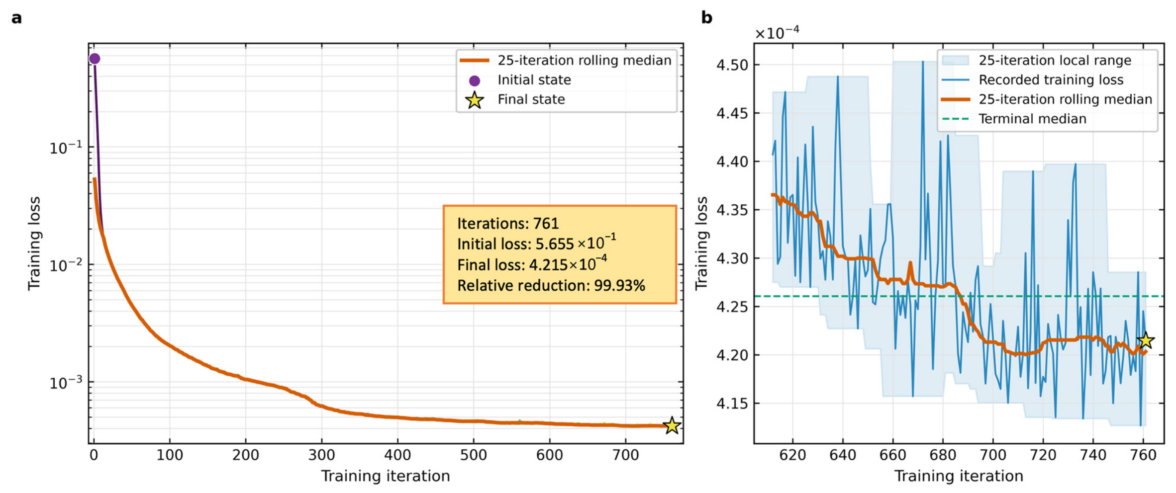
The prediction performance of the proposed ANN was evaluated on the geometry-grouped independent test subset using the performance metrics and validation procedures described in Figure 4, which illustrates the training convergence history of the proposed ANN. The training loss decreased from 5.655 × 10⁻¹ to 4.215 × 10⁻⁴ over 761 training iterations, corresponding to an overall reduction of approximately 99.93%. Most of the loss reduction occurred during the early stages of training, whereas subsequent iterations produced progressively smaller improvements as optimisation approached convergence. The 25-iteration rolling median was included to reveal the underlying convergence tendency while reducing the visual influence of short-term stochastic fluctuations associated with mini-batch optimisation.

The enlarged view of the final training stage shows that the loss fluctuated within a narrow range while the rolling median remained nearly constant. These small oscillations are consistent with the stochastic nature of the Adam optimizer and do not indicate optimisation instability or divergence. The convergence history therefore demonstrates that the training process reached a stable low-loss region before termination, indicating that the reported independent test performance reflects the predictive capability of the trained network rather than incomplete optimisation.

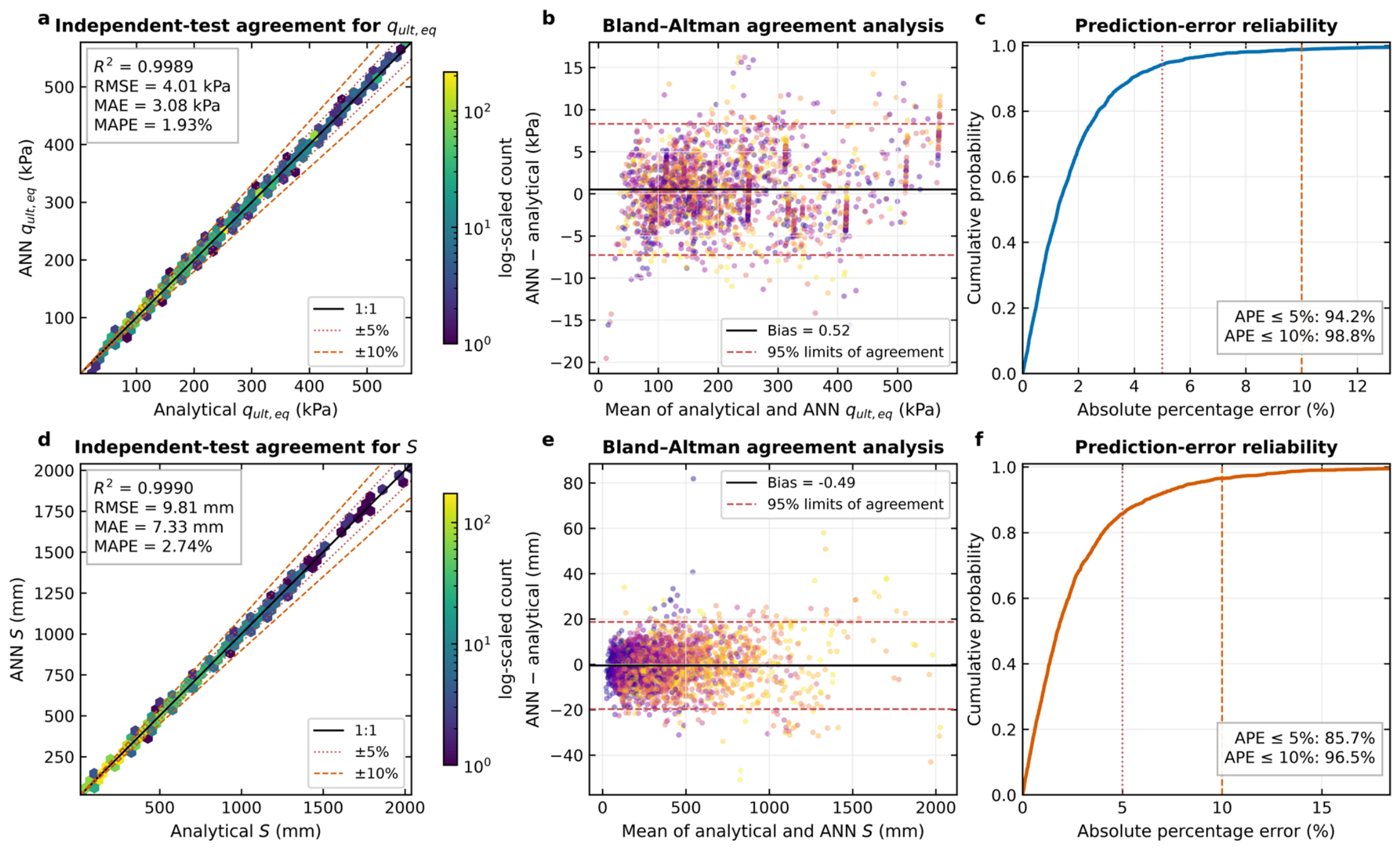
Figure 5 summarises the ANN performance on the independent test subset. The predicted equivalent ultimate grid pressures closely followed the analytical targets, yielding R² = 0.9989, RMSE = 4.01 kPa, MAE = 3.08 kPa, and MAPE = 1.93%. The Bland–Altman analysis indicated a negligible bias of 0.52 kPa, with approximate 95% limits of agreement from −7.28 to 8.32 kPa. Moreover, 94.2% and 98.8% of the test predictions exhibited absolute percentage errors not exceeding 5% and 10%, respectively.

Similarly, the ANN reproduced the analytical settlement response with R² = 0.9990, RMSE = 9.81 mm, MAE = 7.33 mm, and MAPE = 2.74%. The mean ANN–analytical difference was 0.49 mm, and the approximate 95% limits of agreement ranged from −19.70 to 18.72 mm. Absolute percentage errors remained below 5% for 85.7% of the test samples and below 10% for 96.5%. Although the dispersion of the paired differences increased moderately with settlement magnitude, no systematic trend or magnitude-dependent prediction bias was observed, indicating that the ANN maintained stable predictive accuracy throughout the investigated design space.

The output-specific permutation-sensitivity analysis revealed distinctly different input-dependence patterns for the two ANN outputs. For equivalent ultimate grid pressure, q_ult,eq, column spacing was the most influential input, accounting for 42.18% of the total normalised sensitivity, followed by column diameter (24.62%), column length (19.10%), and undrained shear strength (14.09%). Soil-constrained modulus and applied raft pressure each contributed less than 0.01% to this output. Conversely, settlement was governed primarily by column length (47.02%), applied raft pressure (30.40%), and soil-constrained modulus (20.78%), while column diameter (1.09%), column spacing (0.71%), and undrained shear strength had comparatively minor effects. These contrasting rankings are mechanically consistent with the analytical formulations used to generate the ANN targets: grid resistance depends principally on column geometry and undrained soil strength, whereas settlement depends mainly on treatment depth, applied loading, and composite ground stiffness. The results thus provide an output-specific quantitative interpretation of the final 6–24–12–2 ANN within the investigated analytical domain.

These sensitivity results should be interpreted within the prescribed analytical parameter domain. Because the ANN is trained on responses generated from the analytical formulations, the permutation sensitivities describe the relative dependence of the surrogate predictions on each input over the investigated ranges. They are therefore used as a complementary interpretability measure and should not be interpreted as universal rankings of the governing factors in field-scale jet grout behaviour.

5.2. Comparison of ANN and Linear Regression Prediction Performance

Although the comparison with the analytical targets demonstrated that the proposed ANN accurately reproduced the underlying analytical response, its practical value also depends on whether it provides a meaningful improvement over simpler predictive models. Accordingly, to assess the benefit of nonlinear learning, the predictive performance of the proposed ANN was compared with that of a linear regression model developed using the same input variables together with the identical geometry-grouped training and independent test datasets. 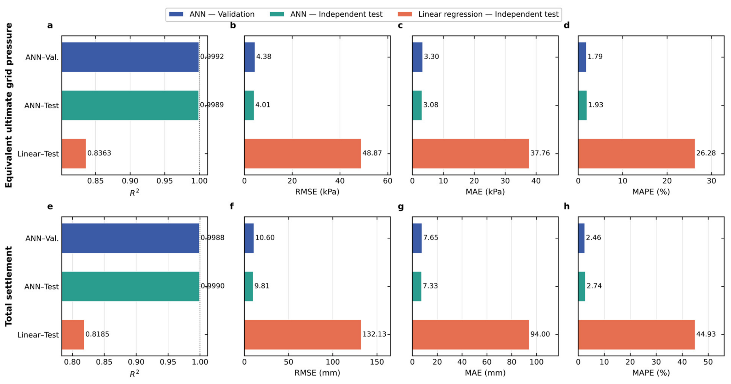Figure 6 summarises the prediction performance of both models for the equivalent ultimate column-grid pressure and total settlement.

As shown in Figure 6, the proposed ANN achieved consistently high predictive accuracy for both equivalent ultimate column-grid pressure and total settlement. For both response variables, the validation and geometry-grouped independent test subsets yielded closely comparable performances, with coefficients of determination exceeding 0.998 and MAPE values below 3%. The close agreement between the two datasets indicates that the proposed ANN generalised successfully to previously unseen jet grout geometries without any measurable degradation in predictive performance. In contrast, linear regression produced considerably lower coefficients of determination and substantially larger errors. For equivalent ultimate grid pressure, linear regression yielded R² = 0.8363 and MAPE = 26.28%, while for settlement, it yielded R² = 0.8185 and MAPE = 44.93%. Relative to linear regression, the independent test ANN reduced the RMSE by approximately 91.8% for equivalent ultimate grid pressure and 92.6% for settlement. The corresponding MAE reductions were approximately 91.8% and 92.2%.

To evaluate the surrogate directly at the engineering decision level, ANN-based and exact analytical feasibility classifications were compared for all 2400 cases in the geometry-grouped independent test set using FS_req = 3.0 and S = 75 mm. The two approaches produced identical classifications for 2387 cases, corresponding to an overall decision agreement of 99.46%. Only 11 cases (0.46%) were classified as false feasible by the ANN, while 2 cases (0.08%) were classified as false infeasible. Importantly, the ANN-based and analytical screening procedures identified the same minimum-treatment-intensity feasible configuration in the design application. Thus, the limited classification differences did not affect the final geometry selected by the performance-based screening procedure.

5.3. Application of the Proposed Framework to Representative Design Cases

The practical applicability of the proposed framework was demonstrated by applying the trained ANN to representative combinations of soil properties and foundation loading. For each design case, all candidate diameter–spacing–length (D–s–L) configurations within the investigated design space were evaluated against the prescribed bearing resistance and settlement criteria. The feasible alternatives were subsequently ranked using the treatment-intensity index, and the geometry requiring the minimum treatment intensity was identified as the preferred design.

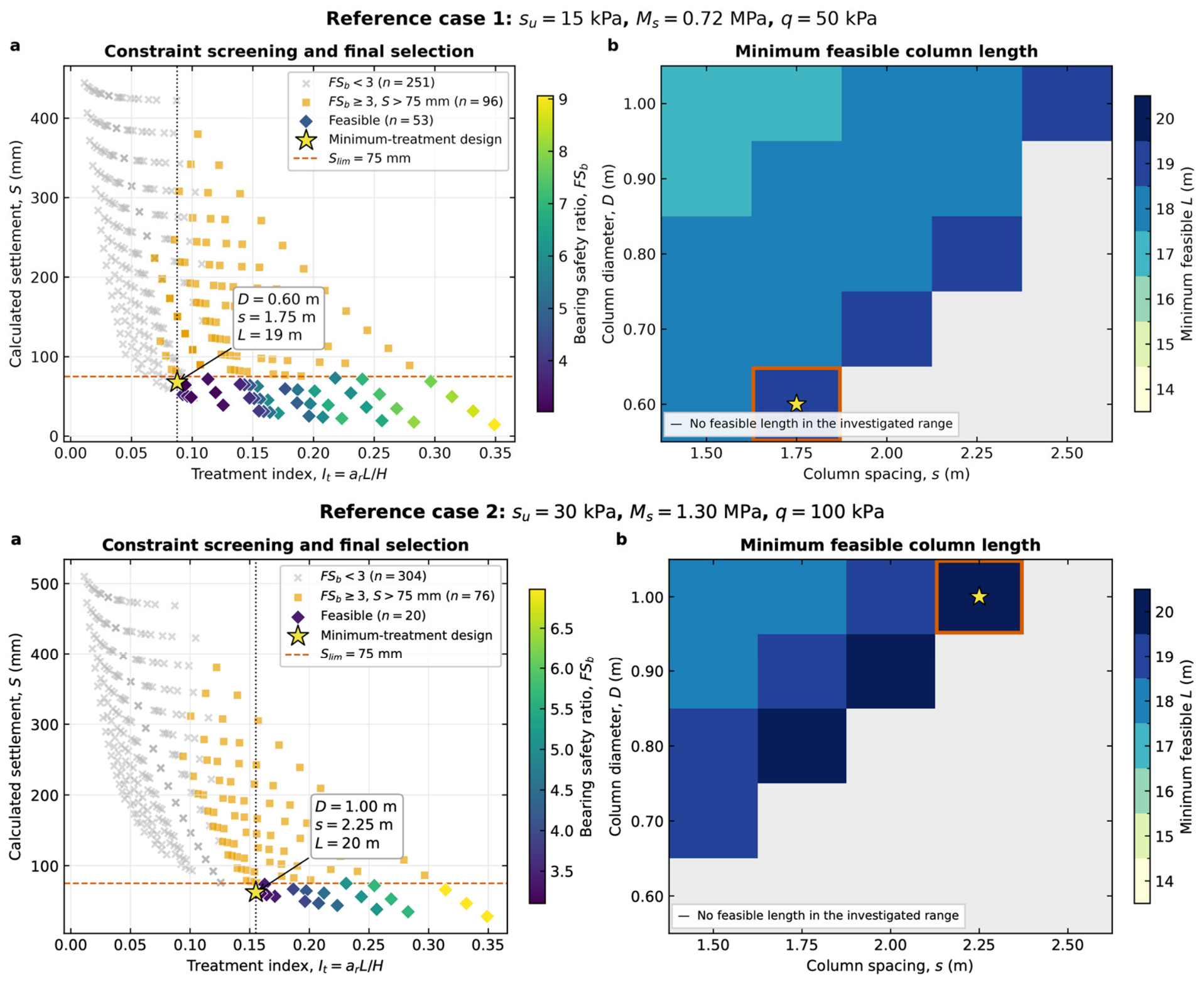
Figure 7 illustrates the resulting performance-based geometry selection procedure for representative soil and loading conditions. For each case, the left-hand panel presents the evaluation of all 400 candidate geometries according to the bearing resistance requirement (FS_b = 3.0) and the allowable settlement criterion (S = 75 mm). Among the feasible alternatives, the configuration with the minimum treatment-intensity index (It) was selected. The right-hand panel shows the minimum feasible column length for each diameter–spacing combination. The selected geometry is identified by the star and orange outline, whereas grey cells indicate diameter–spacing combinations for which no feasible column length was found within the investigated range of 5–20 m. A common colour scale (14–20 m) is used in all cases to facilitate a direct comparison of the required treatment lengths.

As demonstrated in Figure 7, the number of feasible jet grout geometries and the required treatment intensity vary markedly with the combined effects of soil properties and foundation loading. Grey cells indicate that no feasible geometry was identified within the investigated design space. Under the relatively low loading condition of Case 1 (s_u = 15 kPa, M_s = 0.72 MPa, and q = 50 kPa), 53 candidate geometries satisfy both the bearing resistance and settlement constraints, with the preferred solution corresponding to D = 0.60 m, s = 1.75 m, and L = 19 m. Under the intermediate loading condition of Case 2 (s_u = 30 kPa, M_s = 1.30 MPa, and q = 100 kPa), the feasible design space decreases to 20 candidate geometries, and the selected configuration becomes D = 1.00 m, s = 2.25 m, and L = 20 m. These results demonstrate that an increasing foundation demand progressively reduces the number of feasible design alternatives and generally requires larger column diameters together with greater treatment depths to satisfy the prescribed performance constraints. Conversely, lower loading conditions permit a wider range of feasible geometries and lower treatment intensity, providing greater flexibility for preliminary design.

5.4. Finite-Element Assessment of the Proposed Design Solutions

To provide an independent numerical assessment of the settlement component of the proposed framework, two representative design cases were analysed using three-dimensional finite-element (FEM) simulations. The FEM analyses were performed independently of both the analytical data-generation procedure and the ANN training process and therefore provide an independent continuum-mechanics assessment of the proposed settlement.

The two FEM cases provide independent continuum-mechanics assessments of the settlement response for representative configurations selected through the performance-based screening procedure. Their purpose is to examine the mechanical consistency of the analytical and ANN settlement predictions at selected design points rather than to establish exhaustive numerical validation across the complete six-dimensional parameter domain. The present numerical assessment therefore remains limited with respect to the range of treatment lengths, area replacement ratios, soil conditions, and loading levels considered, particularly for floating-column configurations in which compression of the untreated clay beneath the column tips may become increasingly significant. A systematic FEM assessment covering these variations represents an important extension of the present framework.

The analytical and FEM models represent the improved foundation system at different levels of idealisation. The analytical formulation uses a homogenised composite representation within the treated zone and a full-raft stress-spread approach beneath the column tips, whereas the FEM unit cell explicitly represents a column and its tributary soil volume. Accordingly, the FEM simulations provide complementary three-dimensional assessments of the settlement response rather than direct numerical reproductions of the analytical formulation.

The finite-element analyses were performed using PLAXIS 3D 2024.2. The lateral boundaries were restrained normal to their planes and free vertically, while the bottom boundary was fixed vertically. The horizontal dimensions of the unit cell were equal to the centre-to-centre column spacing, s. A single cylindrical jet grout column was placed at the centre of the unit cell. The soil and column domains were discretised using 10-noded tetrahedral elements with a global mesh coarseness factor of 0.075. The software’s automatic mesh generator was employed to obtain a geometry-conforming discretisation, resulting in a locally finer element distribution in the vicinity of the jet grout column and the surrounding soil–column transition region. The same mesh-generation procedure was consistently applied to both reference cases. The initial stress state was generated using the K₀ procedure. A value of K₀ = 1.0 was adopted for the undrained clay. Following the initial-stress calculation, a uniformly distributed vertical pressure, q, was applied over the entire upper surface of the unit cell. The resulting settlement was evaluated using the maximum magnitude of the calculated vertical displacement, |u_z|_max.

The clay behaviour was represented using the Mohr–Coulomb constitutive model. The friction and dilatancy angles were both set to zero, while the cohesion was set equal to the specified undrained shear strength. The constrained modulus, M_s, was used in the analytical calculation of the settlement contribution below the jet grout columns because this component was formulated under one-dimensional compression conditions. In the finite-element analyses, M_s was not assigned directly as a material parameter. Instead, the soil stiffness in the finite-element model was defined using Young’s modulus, Es, together with Poisson’s ratio, ν_s, as required for the elastic component of the Mohr–Coulomb constitutive model, with the corresponding constrained modulus. Accordingly, the analytical and finite-element formulations employed stiffness parameters consistent with the underlying assumptions of their respective modelling approaches. The unsaturated and saturated unit weights of the clay were set to 18 and 19 kN/m³, respectively. Poisson’s ratio was taken as ν_s = 0.495 to approximate an incompressible undrained response. The jet grout column was modelled as a nonporous Mohr–Coulomb continuum with an elastic modulus of E_jg = 200 MPa, Poisson’s ratio of ν_jg = 0.20, unit weight of γ_jg = 21 kN/m³, and cohesion of c_jg = 1000 kPa. The column friction and dilatancy angles were set to zero. Complete displacement compatibility was assumed between the jet grout columns and the surrounding soil.

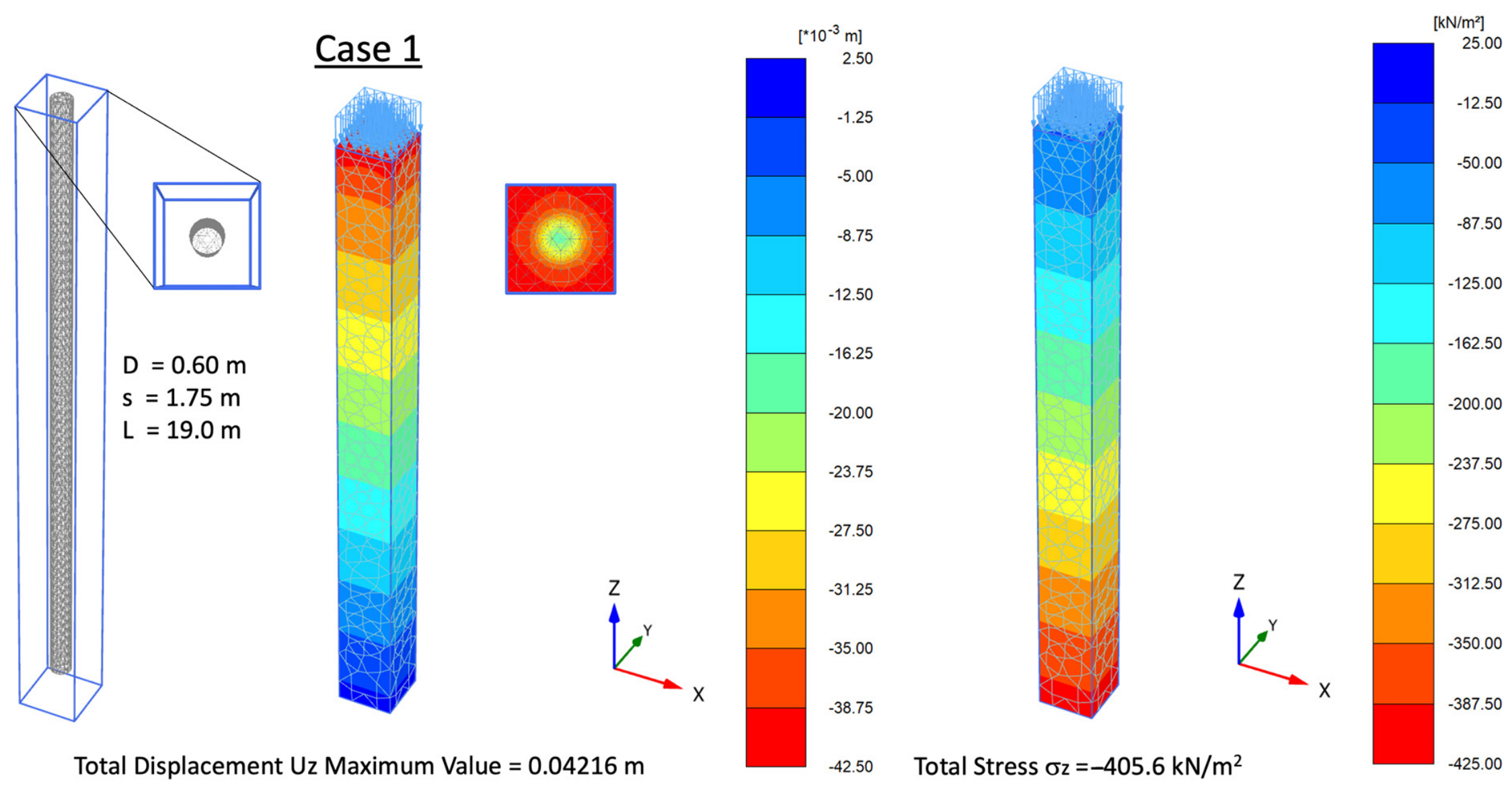
Reference Case 1, illustrated in Figure 8, represented a relatively soft-to-medium clay subjected to a surface pressure of 50 kPa. The soil parameters were s_u = 15 kPa and M_s = 0.72 MPa. The selected jet grout configuration consisted of columns with a diameter of D = 0.60 m, centre-to-centre spacing of s = 1.75 m, and length of L = 19 m.

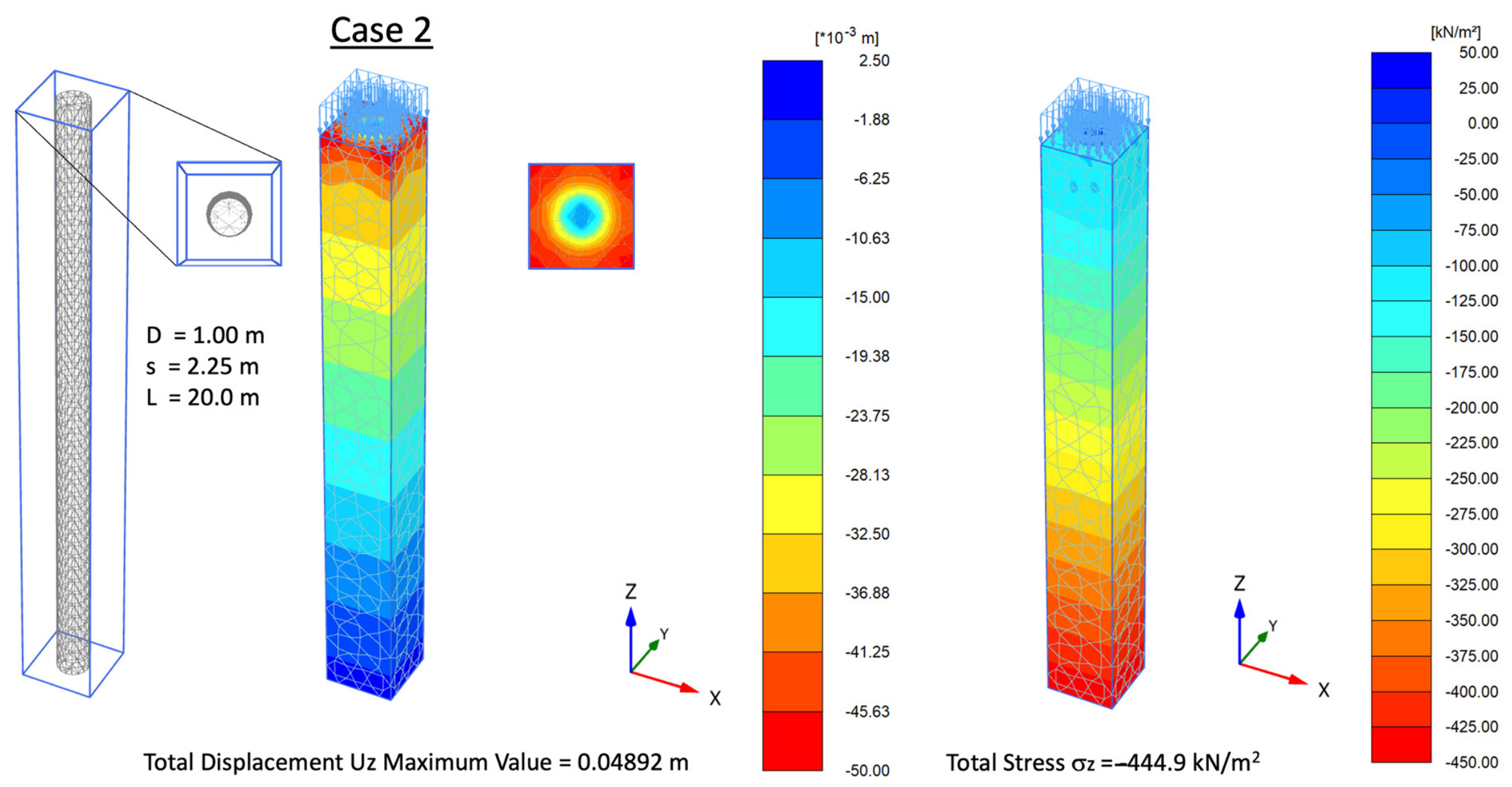
Figure 9 presents reference Case 2, representing a stronger and stiffer clay subjected to a higher surface pressure. The adopted parameters were s_u = 30 kPa, M_s = 1.30 MPa, and q = 100 kPa. The selected column geometry was D = 1.00 m, s = 2.25 m, and L = 20 m.

The finite-element analyses resulted in maximum vertical settlements of 42.16 mm for Case 1 and 48.92 mm for Case 2. The corresponding analytical settlements were 67.59 and 62.25 mm, whereas the ANN predictions were 60.37 and 67.69 mm, respectively.

Both the analytical formulation and the ANN produced conservative settlement estimates relative to the FEM results. For Case 1, the analytical and ANN predictions exceeded the finite-element settlement by 60.3% and 43.2%, respectively. The ANN prediction was therefore closer to the FEM result than the analytical estimate for this case, although both approaches retained the same conservative response tendency. Closer agreement between the analytical and finite-element results was obtained for Case 2. The analytical settlement exceeded the FEM result by 27.3%, whereas the ANN prediction exceeded it by 38.4%. Nevertheless, the analytical and ANN predictions remained reasonably close, differing by approximately 8.7%. This correspondence is consistent with the role of the ANN as a surrogate trained using responses generated by the analytical formulation. Across both reference cases, the mean absolute differences relative to the FEM results were approximately 19.38 mm for the analytical formulation and 18.49 mm for the ANN. The ANN therefore reproduced the conservative tendency of the analytical response generator without introducing a substantial additional discrepancy in the settlement estimates.

The differences between the analytical and finite-element results reflect the distinct modelling assumptions of the two approaches. The analytical formulation represents the improved ground using equivalent relationships, whereas the FEM model explicitly represents the three-dimensional soil and jet grout column volumes. Further differences may arise from the finite-element boundary conditions, the assumption of compatible deformation between the columns and surrounding soil, the omission of explicit interface slip, the assumed nonporous behaviour of the columns, and the elastic–perfectly plastic representation of the clay through the Mohr–Coulomb model.

6. Discussion

The proposed ANN demonstrated consistently high predictive performance because the underlying analytical response generator is governed by strongly nonlinear interactions between soil properties, loading conditions, and jet grout geometry. Equivalent ultimate column-grid resistance is controlled by nonlinear and piecewise relationships involving column cross-sectional area, shaft resistance, end-bearing resistance, material strength limitations, and the governing minimum of the geotechnical and material resistance components. Likewise, settlement depends on the coupled influence of the area replacement ratio, equivalent composite stiffness, applied foundation pressure, treatment depth, and the thickness of the untreated clay layer. These coupled mechanisms introduce multiplicative, inverse, threshold-dependent, and interaction effects that cannot be represented adequately by a simple additive linear model. Consequently, the substantial improvement achieved by the ANN over linear regression demonstrates its ability to reproduce the strongly nonlinear response relationships embedded in the analytical framework.

While individual analytical evaluations for a single jet grout configuration are computationally inexpensive, the iterative processing of multidimensional design matrices within complex optimisation loops or parametric screening routines can increase computational overheads in large parametric screening routines. The developed physics-generated ANN surrogate effectively translates the coupled closed-form expressions into a unified, vectorized matrix mapping system. This configuration provides a unified prediction interface for repeated screening of candidate geometries while simultaneously estimating bearing resistance and settlement. As emphasised in recent geotechnical machine learning literature [8,10,11], utilising such physics-consistent surrogates yields critical functional advantages, particularly in rendering interactive decision-support tools and automated screening interfaces operational without heavy software dependencies. Crucially, this setup establishes a scalable numerical framework that directly accepts higher-fidelity response data—such as finite-element outputs or experimental field datasets—without modification to the downstream performance-based geometry selection protocol.

The close agreement between the validation and geometry-grouped independent test results further indicates that the proposed ANN learned the governing response relationships rather than memorising individual design configurations. The geometry-grouped partition prevented identical diameter–spacing–length combinations from appearing in multiple subsets, thereby providing a more rigorous assessment of generalisation than conventional random row-wise partitioning. Furthermore, the negligible Bland–Altman biases and narrow limits of agreement indicate that the ANN reproduced the analytical response without introducing systematic overprediction or underprediction throughout the investigated design space.

Although prediction accuracy remained consistently high for both outputs, settlement exhibited a slightly greater relative error and a moderate increase in residual dispersion at larger response magnitudes. This behaviour is expected because settlement depends on several coupled deformation mechanisms that accumulate throughout the treated and untreated soil profiles, whereas the equivalent bearing resistance is primarily governed by resistance mobilisation within the jet grout columns. Future developments could therefore investigate response transformations, loss functions, or adaptive enrichment of the high-settlement region to further improve prediction accuracy for larger settlements.

From an engineering perspective, the principal contribution of the proposed framework is not merely the development of an accurate ANN surrogate but the integration of transparent analytical formulations with performance-based geometry selection. Rather than predicting a single response quantity, the trained ANN simultaneously evaluates bearing resistance and settlement for every candidate geometry within the investigated design space and rapidly identifies feasible jet grout configurations that satisfy prescribed performance requirements. This provides a unified prediction interface for repeated evaluations of candidate geometries while maintaining consistency with the underlying analytical formulation.

The independent finite-element assessment provides a complementary numerical comparison of the settlement response predicted by the proposed framework. The differences between the analytical/ANN predictions and FEM results should be regarded as substantial in terms of settlement magnitude, particularly for Case 1, rather than as close quantitative agreement. Nevertheless, the analytical, ANN-predicted, and FEM settlements all remained below the illustrative settlement limit of 75 mm for both cases; therefore, the observed numerical differences did not alter the settlement-based feasibility classification of these particular configurations. The discrepancies reflect the different representations of stress redistribution, treated-zone stiffness, boundary conditions, constitutive behaviour, and soil–column compatibility adopted in the analytical and finite-element formulations. Because the ANN was trained exclusively using analytically generated responses, the FEM comparison should be interpreted as an independent numerical assessment of the settlement response rather than as physical validation of the ANN or the complete proposed framework.

More broadly, geotechnical and earthquake engineering are increasingly evolving towards data-driven design frameworks in which machine learning methods complement conventional analysis by integrating multidimensional information from field investigations, laboratory testing, monitoring, and numerical simulations [34,35,36]. As such datasets continue to expand, physics-guided and data-driven models are expected to play an increasingly important role in identifying complex parameter interactions and supporting prediction-, interpretation-, and performance-based engineering decisions.

Consequently, the proposed framework should be regarded as a transparent and reproducible preliminary design tool rather than a substitute for project-specific numerical analysis or field verification. Future research should extend the database by using calibrated laboratory and field observations, incorporate advanced constitutive soil models, and further examine the robustness of the framework through comprehensive sensitivity and uncertainty analyses.

7. Conclusions

This study presented a physics-generated artificial neural network (ANN) framework for the preliminary performance-based design of jet grout columns beneath raft foundations constructed on soft-to-medium clays. The proposed framework integrates transparent analytical formulations with machine learning to simultaneously evaluate equivalent bearing resistance and settlement while efficiently identifying feasible jet grout geometries that satisfy prescribed performance requirements.

The developed ANN successfully reproduced the nonlinear behaviour of the underlying analytical framework and demonstrated robust generalisation to previously unseen design configurations. The comparison with multiple linear regression further confirmed that the nonlinear ANN provides a substantially more accurate representation of the coupled soil–structure response governing jet grout design. Application of the trained ANN to representative design cases demonstrated its capability to efficiently evaluate hundreds of candidate geometries and rapidly identify the minimum treatment solution satisfying both bearing resistance and settlement constraints.

Independent three-dimensional finite-element analyses provided additional confidence in the engineering consistency of the proposed framework. Although quantitative differences were observed between the analytical/ANN estimates and the FEM results, all three approaches produced the same settlement-based feasibility classification for the representative cases. These findings indicate that the proposed ANN preserves the mechanical characteristics of the analytical formulation while offering a computationally efficient surrogate suitable for preliminary engineering design within the investigated preliminary design domain.

The proposed framework should be interpreted within the scope of the adopted analytical assumptions and investigated parameter ranges. Accordingly, it is intended as a transparent and reproducible preliminary design tool rather than a replacement for project-specific numerical analyses, field testing, or detailed design verification. Future work should focus on extending the analytical database through laboratory and field calibrations, incorporating advanced constitutive soil models and explicit soil–column interface behaviour, expanding the investigated design space, and evaluating the methodology under more complex geological and loading conditions.