In Situ Thermal Performance Assessment of a Wood–Aluminum Window: Case Study of Spatial Variability, Dynamic Effects, and U-Value Accuracy

Abstract

This paper presents an experimental evaluation of the thermal performance of a wood–aluminum window installed in a timber building exposed to real climatic conditions. The assessment is based on long-term in situ measurements of heat flux and temperature variations. The aim of the research was to determine the thermal transmittance of individual parts of the window assembly, analyze their dynamic thermal behavior, and identify critical areas in terms of heat losses. The results revealed a spatially heterogeneous distribution of heat fluxes through the window structure. The center of the glazing achieved values close to the declared U_g parameter, whereas the edge regions of the glazing and the window frame exhibited a significant increase compared with the declared values. The time-dependent analysis confirmed a distinct diurnal cycle of heat flux and a phase shift between the glazing and frame components. Furthermore, it was demonstrated that the accuracy of local U-value determination is significantly affected by the magnitude of the temperature difference, with the stability and repeatability of the calculated U-values improved at higher ΔT values, particularly above approximately 10–15 K. The findings highlight the need for detailed, spatially resolved assessment of window structures and emphasize the importance of experimental verification of their thermal performance under real conditions.

1. Introduction

The energy performance of buildings remains a key topic in contemporary building research, as the accurate characterization of heat transfer through the building envelope is essential for evaluating operational energy use, designing retrofitting strategies, and validating simulation models. In this context, the thermal transmittance, or U-value, is widely used as a fundamental indicator of the thermal quality of building components. In recent years, increasing attention has been devoted to the gap between design or declared values and the actual in-use performance of building envelope systems. This need has been highlighted by both review-based and experimental studies addressing the in situ assessment of opaque envelope components and transparent elements, including windows and glazing systems [1,2,3,4,5].

Windows represent a specific part of the building envelope, as they simultaneously fulfill daylighting, architectural, operational, and thermal performance functions. This multifunctionality means that their thermal behavior cannot be reduced to a single homogeneous U-value. Several studies have shown that the actual thermal performance of windows depends on a combination of the properties of the glazing, frame, spacer elements, installation joint, installation details, and the method of connection to the building structure. This is reflected particularly in the difference between the central part of the glazing and the edge zones, where heat losses are typically higher and surface temperatures lower due to the distortion of temperature fields [6,7,8,9,10]. These effects may become even more pronounced when vacuum glazing is used [11,12,13,14].

Experimental measurements and numerical simulations have long confirmed that the glazing type itself has a significant effect on the thermal performance of window assemblies. Early analyses of so-called super-insulating windows indicate that the combination of high-performance glazing and a properly designed frame can markedly reduce heat losses under winter operating conditions [15]. More recent studies have further shown that the thermal transmittance of glazing is affected not only by the number of panes, gas filling, and low-emissivity coatings, but also by changing outdoor boundary conditions, particularly external temperature and solar radiation [8,16,17]. From a practical point of view, it is also important that contemporary approaches are gradually moving from laboratory-based determination of thermal parameters toward methods capable of estimating the properties of windows already installed in buildings under real operating conditions [2,6,17].

Several studies have shown that frame sections remain critical zones with respect to heat losses, even when high-performance triple glazing is used. Experimental studies focused on frame optimization have confirmed that appropriate cavity fillings, low-emissivity coatings, and the application of advanced insulating materials can reduce frame thermal transmittance by several tens of percent [18,19]. However, the actual thermal behavior of the frame cannot be evaluated in isolation, since the overall thermal response is governed by the interaction between the frame, the glazing, and the installation detail [7,9,20].

Thermal bridges in the glazing-edge region, frame joints, and window-to-wall connections represent a particularly important issue. Misiopecki et al. [21] used 2D finite-element simulations (THERM 7.0) to evaluate the effect of window position on linear thermal transmittance (LTT) for different wall–window configurations. The results showed that optimal window placement can reduce thermal-bridge losses by more than 50%, with the optimal position depending primarily on the wall construction and location of the insulation. Using 2D FEM simulations (Flixo Energy 8.2), Gendelis et al. [22] optimized the window mounting position and insulation overlap based on ψ-values and internal surface temperatures. They showed that positioning windows at an optimal depth within the insulation layer and overlapping the frame with insulation can reduce thermal bridging by up to approximately 90%, while improving surface temperatures and reducing heating demand. Barnes et al. [23] used 2D and 3D thermal simulations to analyze the ψ-values of window installation details and showed that the window-to-wall thermal bridge depends primarily on the structural detail and frame position, whereas the type and thermal performance of the window itself have a substantially smaller effect on the ψ-value. This finding supports the use of cataloged ψ-values for appropriately defined installation details. Using experimentally validated 3D numerical heat-flow simulations (TRISCO) for more than 400 wall–window configurations, Adamus and Pomada [24] showed that installing the window within the thermal insulation layer substantially reduces thermal bridging. The resulting annual heating demand decreased by at least 10% on average, while the wall and insulation material properties also had to be considered together with the window position. Using PHPP energy-balance calculations combined with 2D FEM simulations in THERM 7.6, Kalbe and Kalamees [25] assessed window-frame properties and installation depth. They showed that frame thermal transmittance and frame width strongly affect heating demand, with effects of up to 42% and 25%, respectively, whereas optimizing the window installation depth has only a minor effect (approximately 3%) because the reduction in thermal bridging is partly offset by reduced solar gains.

Similarly, Qin et al. [26] used steady-state two-dimensional finite-element heat-transfer simulations, validated against manufacturer test data, to compare five window–wall interface designs under climatic conditions representative of Nanjing and a cold-climate region. The study evaluated surface temperatures, condensation risk, heat flux, and heat flow. The newly proposed interface, in which insulation was placed around the sill and near the window-frame thermal bridge, showed the best overall thermal performance, reducing surface heat flow by 42.4% compared with the conventional insulated solution and substantially lowering the risk of condensation. Nôta and Danihelová [27] and Nôta [28] used 2D numerical modeling in THERM 7.6 to evaluate the linear thermal transmittance (ψ) of a wood–aluminum window at multiple installation positions in five different wall constructions. They showed that the optimal window position depends strongly on the wall composition and temperature-field distribution, with the lowest ψ-value generally occurring near the region of minimum thermal-field deformation but shifted by up to approximately 11.5% of the wall thickness. Choi and Ko [29] used five-day in situ heat-flow-meter (HFM) measurements and infrared thermography (IRT) on six exterior walls. They compared several U-value evaluation methods and found that the three HFM-based methods agreed within 10%, whereas IRT-derived U-values differed from the reference HFM method by 6–43%, highlighting the lower reliability of instantaneous IRT measurements due to thermal-inertia effects.

In terms of frame-related and point thermal bridges, the studies by Ben-Nakhi [30] and Terentjevas et al. [31] are also relevant. Ben-Nakhi [30] evaluated thermal bridging and cooling loads for several window–wall configurations under hot-climate conditions and found that thermal bridging in conventional window systems is significant. Extending the insulation around the window edge was identified as the most effective and practical modification for reducing both linear thermal transmittance and cooling loads. Terentjevas et al. [31] used 2D (THERM) and 3D (HEAT3) numerical modeling according to ISO 10211 to evaluate point and linear thermal bridges of windows installed directly within stone-wool insulation. The results showed that 3D modeling is essential for capturing the effects of fasteners and that positioning the window more than 100 mm from the supporting wall can substantially reduce thermal bridging, with reductions of up to 37% compared with conventional installation.

The heat flux method, and particularly the heat flow meter (HFM) approach, is among the most widely used methods for in situ local U-value determination. Its main advantage is the direct measurement of heat flux density. However, the accuracy of the resulting U-value depends on the magnitude of the temperature difference, the measurement duration, the stability of boundary conditions, and the correct determination of both surface and air temperatures. These limitations have been addressed in review papers as well as in experimental studies conducted under different climatic and operating conditions [5,32,33,34]. Therefore, recent studies have compared the HFM method with alternative procedures, including temperature-based methods, low-cost IoT-based solutions, virtual HFM models, and newly developed devices for field measurements [4,29,35,36,37,38,39]. The common conclusion is that longer measurement periods and the careful selection of quasi-stationary intervals improve the reliability of the estimated U-value, whereas small temperature differences and strong dynamic disturbances can result in substantial deviations.

For windows, this issue is even more critical, as they are characterized by the low thermal storage capacity of glazing, a pronounced influence of radiative heat transfer, and a locally highly nonuniform temperature field. In their in situ evaluation of window U-values, study [2] showed that HFM and IR-based approaches can be used in a complementary manner, while emphasizing that the appropriate selection of the measurement location is essential. Study [2] also confirms that the temperature-based method is applicable only under certain temperature-difference conditions and may produce invalid or even negative results when applied under unsuitable boundary conditions. In the review [1], authors concluded that the experimental evaluation of window U-values is methodologically more complex than that of homogeneous opaque elements, as it must account for the effects of edge zones, frames, radiation, installation details, and varying weather conditions. This is consistent with more recent studies focusing directly on glazing systems and windows under real operating conditions, which have shifted attention from single-point measurements toward long-term monitoring and data-driven modeling approaches [10,17].

From a practical design perspective, reducing the overall thermal transmittance of the window, U_w, is not sufficient on its own; the control of local internal surface temperatures is equally important. The link between local detailing and the risk of surface condensation has been documented in both numerical and experimental studies addressing glazing details and window profiles [26,40,41,42]. Moreover, reliable assessment of such details benefits from combining experimental measurements with numerical modeling. While experimental measurements capture the actual thermal response of the construction, numerical models allow the interpretation of isotherm patterns, heat flux concentrations, and the sensitivity of the detail to changing boundary conditions [21,43,44].

Although the current literature provides extensive knowledge on U-value assessment, thermal bridges, and in situ measurement methods, several research gaps remain in the case of windows. Most studies focus either on glazing systems tested under laboratory conditions, general measurement methodologies, or opaque building components such as walls. In contrast, relatively few studies have provided a long-term, spatially resolved analysis of several parts of a single window under real operating conditions, including the center of the glazing, the upper and lower glazing-edge zones, sash and frame sections, and lower frame profiles. Furthermore, limited attention has been paid to interpreting these measurements in relation to local thermal bridges and to the discrepancy between declared and experimentally determined thermal parameters [1,2,7,9,10].

The main research gap lies in the limited availability of long-term in situ studies focused on real installed windows, in which heat fluxes and surface temperatures are spatially resolved across individual window components, including the glazing, frame, and installation detail. Particular attention is required to account for dynamic winter operating conditions. Measurements performed under real conditions allow differences between the central glazing area and critical edge details to be quantified and enable experimental data to be linked with the theoretical interpretation of thermal bridges as well as with manufacturer-declared parameters. This gap arises from existing review and experimental studies, which often address measurement methods or selected aspects of window details, but only rarely provide a comprehensive, long-term, and spatially resolved assessment of a specific window installed in a real building.

The aim of this study is to experimentally analyze the thermal behavior of a wood–aluminum window installed in a timber building using long-term in situ measurements of heat flux and temperature. The objectives are to determine the U-values of selected components of the window assembly, identify regions with elevated thermal losses and internal surface temperatures, and interpret the results in relation to thermal bridges and manufacturer-declared thermal parameters.

The contribution of this study lies in providing detailed experimental data on the thermal behavior of a modern wood–aluminum window installed in a real building under winter operating conditions. By distinguishing the thermal response of individual parts of the window assembly, the study goes beyond the use of a single global U-value and provides a basis for a more accurate interpretation of critical components. Furthermore, the results can serve as experimental input for the validation of numerical models and may support practical design decisions in the development of nearly zero-energy buildings.

The study was intentionally designed as an in situ case study of a single wood–aluminum window assembly rather than as a comparative investigation of different window materials or climatic regions. This approach enabled the spatial variability of thermal performance within the same window to be examined while maintaining identical construction and installation conditions. The investigated window is permanently installed in an experimental building in Zvolen, Slovakia; therefore, the measurements represent naturally varying winter conditions characteristic of its Central European location. Consequently, the numerical results are specific to the investigated window assembly and boundary conditions and should not be interpreted as universally representative values for all wood–aluminum windows or climatic regions.

2. Materials and Methods

2.1. Investigated Window and Installation Detail

The experimental assessment of the thermal performance of the window assembly was conducted in situ on a MINTAL (Mintal s.r.o., Sielnica, Slovakia) Classic wood–aluminum window installed in a prototype research building of the Department of Wooden Constructions at the Technical University in Zvolen, Slovakia (Figure 1). The window was fitted with SGG Climatop XN triple glazing (Glasora a.s., Nira, Slovakia) fitted with a warm swisspacer frame (SWISSPACER Vetrotech Saint-Gobain International AG, Lengwil, Switzerland). The investigated assembly was exposed to natural climatic conditions, enabling the analysis of its behavior under both quasi-stationary and transient regimes, which are typical of building operation in the Central European climate.

For improved reproducibility of both the experimental assessment and the numerical model, the principal geometric and material characteristics of the investigated window assembly are summarized in

Table 1. Main geometric and material characteristics of the investigated wood–aluminum window assembly.

Parameter	Specification
Window type	Wood–aluminum window
Overall window dimensions	1230 × 1480 mm
Timber frame material	Glued laminated spruce
Frame profile depth	88 mm
Exterior frame protection	Aluminum profile
Glazing type	Triple insulating glazing, SGG CLIMATOP XN
Glazing configuration	8–14–4–14–8 mm
Gas cavities	Argon, ≥90%
Spacer	Swisspacer warm-edge
Glazing dimensions	998 × 1228 mm
Sash/frame characteristic dimensions	51/61 mm
Installation frame dimensions	1280 × 1530 mm
Load-bearing wall	120 mm MHM panel
Installation joint insulation	Wood-fibre-based thermal insulation
Window position	In the thermal-insulation plane, outboard of the MHM panel

. The dimensions refer to the actual window specimen investigated in this study.

The window was installed in the wall on a base of MHM panels (MHM Slovakia, Bytča, Slovakia) (Figure 2). The installation joint was filled with wood-fiber-based thermal insulation and sealed using SIGA Fentrim IS 20 (SIGA Cover AG, Ruswil, Switzerland) sealing tape on the interior side and SIGA Fentrim IS 2 sealing tape on the exterior side. For measurement purposes, the interior reveal was exposed and left without the final interior finish or cladding. According to the manufacturer’s declared data, the thermal transmittance of the glazing was U_g = 0.63 W·m⁻²·K⁻¹, the frame thermal transmittance was U_f = 1.09 W·m⁻²·K⁻¹, and the overall window thermal transmittance was U_w = 0.67 W·m⁻²·K⁻¹ for a window size of 1230 × 1480 mm.

2.2. Experimental Setup and In Situ Measurements

The experimental setup was designed to enable simultaneous monitoring of heat flux density and surface temperatures at representative locations of the investigated window assembly, thereby capturing spatial differences in its thermal behavior under real operating conditions.

Figure 1. Experimental setup of the measured window: (left) arrangement of sensors on the window; (central) detailed view of sensors installed at the lower edge of the glazing; (right) cross-section of the window assembly showing the lower profiles of the frame and sash.

Figure 1. Experimental setup of the measured window: (left) arrangement of sensors on the window; (central) detailed view of sensors installed at the lower edge of the glazing; (right) cross-section of the window assembly showing the lower profiles of the frame and sash.

Figure 2. Side installation details of the wood–aluminum window in the external wall of the research building constructed from MHM panels.

Figure 2. Side installation details of the wood–aluminum window in the external wall of the research building constructed from MHM panels.

The measurements were designed to determine the heat flux density q (W·m⁻²) passing through individual parts of the window assembly and, at the same time, to monitor temperature variations in the indoor and outdoor environments as well as at selected surface locations of the construction. The measurements were performed using an ALMEMO 2890-9 data acquisition system (Ahlborn GmbH, Holzkirchen, Germany) equipped with ALMEMO FQAD17T heat flux sensors with dimensions of 100 × 30 mm and type K thermocouples. All sensors used were calibrated by the manufacturer. The heat flux sensors were applied to the interior side of the window assembly at several representative locations: at the center of the glazing, at the upper and lower glazing edges adjacent to the sash frame, on the window sash, and in the lower frame area near the reveal (Figure 3). This arrangement enabled local variations in heat flux to be captured and allowed the thermal behavior of individual parts of the window assembly to be assessed separately. Thermal paste was used to reduce the contact thermal resistance between each heat flux sensor and the surface of the construction, thereby minimizing measurement errors caused by imperfect thermal contact. Thermocouples were installed at the corresponding surface locations of the window and in the air approximately 200 mm from the surface in order to record indoor and outdoor air temperatures.

2.3. Measurement Conditions and Data Evaluation

2.3.1. U Value

The measurements were conducted between 17 January and 27 February 2024, with data recorded at 10 min intervals (more than 1350 measurements). During the measurement period, the average indoor temperature was 20.81 ± 0.49 °C, corresponding to standard indoor environmental conditions according to STN 73 0540-2:2019 [45]. The outdoor boundary conditions varied throughout the monitoring period, enabling the thermal behavior of the window assembly to be analyzed under different temperature regimes. The outdoor air temperature ranged from −8 to +13 °C, and both quasi-stationary and distinctly transient thermal states were observed. The thermal transmittance was evaluated according to Equation (1), derived from the definition of heat flux:

$$U={\displaystyle \frac{q}{(T_{\mathrm{i}}-T_{\mathrm{e}})}}$$

(1)

where q denotes the measured heat flux density (W·m⁻²), and T_i − T_e represents the temperature difference between the indoor and outdoor air temperatures (K). This approach, based on the heat flow meter method, is commonly used for the in situ determination of the thermal transmittance of building components under real conditions (ISO 9869-1, 2014 [46]). The U-values derived from the HFM measurements represent local apparent thermal transmittance at the specific sensor locations and therefore characterize local heat-transfer conditions rather than the area-weighted thermal performance of the complete window. They should not be interpreted as standardized U_g, U_f or U_w values. In particular, U_w represents the overall thermal transmittance of the complete window, accounting for the area-weighted contributions of glazing and frame as well as the linear thermal transmittance of the glazing edge. Consequently, comparisons between the measured local apparent U-values and manufacturer-declared values are used only as a reference for assessing the consistency and relative thermal performance of the investigated regions and not as a direct equivalence between the quantities.

2.3.2. Uncertainty

The expanded uncertainty of the calculated U-values was qualitatively estimated from the manufacturer-specified accuracies of the heat flux sensors (±5%) and thermocouples (±0.5 K), using Equation (2):

$$u(U)=\sqrt{{\left({\displaystyle \frac{u\left(q\right)}{\mathsf{\Delta }T}}\right)}^2+{\left({\displaystyle \frac{q·u\left(\mathsf{\Delta }T\right)}{{\mathsf{\Delta }T}^2}}\right)}^2}$$

(2)

The uncertainty of the calculated local apparent U-values was evaluated according to the law of propagation of uncertainty following the GUM approach. The manufacturer-specified accuracies of the heat flux sensors (±5%) and thermocouples (±0.5 K) were treated as Type B uncertainty contributions. As no probability distribution or confidence level was specified by the manufacturer, rectangular distributions were assumed, resulting in standard uncertainties of $u\left(q\right)=0.05q/\sqrt{3}$ and $u\left(T\right)=0.5/\sqrt{3}$ K. The standard uncertainty of the indoor–outdoor temperature difference was calculated as $u\left(\mathsf{\Delta }T\right)={\left[u^2\left(T_i\right)+u^2\left(T_e\right)\right]}^{1/2}$. For $U=q/∆T$, the combined standard uncertainty was subsequently determined using Equation (2). The expanded uncertainty was calculated as $U_{\mathrm{e}\mathrm{x}\mathrm{p}}=k{u}_c\left(U\right)$, using a coverage factor of $k=2$, corresponding approximately to a 95% coverage probability. This propagated uncertainty therefore represents the contribution associated with the measurement instruments and should not be interpreted as the complete uncertainty of the in situ U-value determination. The estimated expanded uncertainty (k = 2) determined based on the accuracy of the sensors used is approximately 8% for ΔT > 15 K.

Additional sources of uncertainty inherent to in situ heat-flux measurements were considered. These include sensor positioning, thermal contact between the heat-flux sensor and the measured surface, local spatial heterogeneity of the window components, radiative effects, fluctuations in environmental boundary conditions, and the procedure used for selecting and processing quasi-stationary data. Because independent quantitative estimates were not available for all of these contributions, they were not included numerically in Equation (2) and are discussed separately as methodological uncertainty sources. Their effects were minimized through the use of calibrated sensors, thermal paste to reduce sensor–surface contact resistance, fixed representative sensor positions, preferential analysis of night-time and quasi-stationary periods, and long-term repeated measurements.

2.3.3. Thermal Performance Under Transient Conditions

To obtain representative temporal heat-flux profiles (Figure 4), complete daily cycles were extracted from the measurement dataset and processed separately for each measurement location. Prior to averaging, the individual daily heat-flux curves were temporally aligned by shifting each daily profile so that its maximum heat-flux value occurred at a common reference time. The synchronized profiles were subsequently averaged point by point to obtain a representative 24 h profile for each measurement location. This synchronization was applied solely for visualization and comparison of the characteristic shape and magnitude of the daily heat-flux profiles and was not used for the determination of the thermal time lag. Consequently, the original temporal relationships between the signals are intentionally not preserved in Figure 4. Phase shifts were evaluated independently from the original, non-shifted time series using the procedure described in Section 3.3.

2.3.4. Sensitivity Analysis

The influence of the data-processing procedure was additionally quantified by a sensitivity analysis. Varying the minimum evaluation duration between 4 and 8 h and the heat-flux stability threshold between 3% and 10% produced maximum changes in the calculated local apparent U-values of 2.20% and 0.83%, respectively, indicating that the principal results were only weakly sensitive to the adopted data-selection procedure.

Unless otherwise stated, values reported with the ± symbol in the tables represent the arithmetic mean ± standard deviation (SD) of the measurements within the analyzed time interval and should not be interpreted as measurement uncertainty or confidence intervals.

Owing to the transient nature of the measurements, the data were analyzed using two approaches. First, the complete measured dataset was evaluated to describe the overall thermal response of the window assembly under real operating conditions. Second, selected time intervals fulfilling quasi-stationary conditions were analyzed separately. For the purpose of identifying relatively stable periods within the long-term dataset, quasi-stationary intervals were operationally defined using a 5% heat-flux stability criterion. Because short-term fluctuations were present in the 10 min data, stability was assessed using time-averaged heat flux rather than requiring every individual measurement to remain within ±5% of the interval mean. Each candidate interval was divided into two equal time segments, and the mean heat flux of each segment was required to deviate by less than 5% from the mean heat flux of the complete interval. A minimum duration of 6 h was adopted for the primary analysis. The 5% criterion was selected as a restrictive stability threshold consistent with the convergence concept used in HFM-based thermal performance assessment, while the 6 h duration was considered appropriate for the relatively low thermal inertia of the investigated window assembly. The criterion was used as an operational data-selection procedure and should not be interpreted as the formal convergence criterion specified by ISO 9869-1. To evaluate the influence of the selected interval duration, a sensitivity analysis was additionally performed using otherwise identical 4, 6, and 8 h evaluation periods.

Heat-flux stability was selected as the primary screening variable because heat flux is the directly measured quantity entering the numerator of the local apparent U-value calculation and responds sensitively to transient changes in the thermal state of the lightweight window assembly. A stable heat-flux level was therefore used as a practical indicator that periods dominated by pronounced transient behavior had been excluded. However, heat-flux stability alone was not interpreted as evidence of standardized steady-state conditions. The corresponding indoor and outdoor temperatures and their difference were also examined to ensure that the selected periods did not contain pronounced changes in the thermal driving potential.

2.3.5. Time Lag

The dynamic time lag was initially evaluated using a peak-based approach. For each selected daily period, cubic-spline interpolation was applied to the 10 min outdoor-temperature and heat-flux data to obtain continuous representations of the measured signals. Local extrema were identified from the interpolated curves, and the peak-based delay was calculated as the time difference between the minimum outdoor temperature and the subsequent maximum outward heat flux.

To provide a more objective estimate that does not depend on the identification of individual extrema, a normalized cross-correlation analysis was subsequently performed between the outdoor-temperature and heat-flux signals. The analysis was conducted separately for each complete daily record, considering positive heat-flux lags from 0 to 240 min. The lag corresponding to the maximum correlation coefficient was taken as the characteristic response delay. Because the original data were recorded at 10 min intervals, the cross-correlation lag has a temporal resolution of 10 min. Variability of the estimated lag was evaluated from the results obtained on different measurement days.

2.3.6. Influence $∆T$ on U-Value

To evaluate the influence of the indoor–outdoor temperature difference on the calculated local apparent U-value, each individual measurement record was processed separately. For every 10 min measurement step, the instantaneous indoor–outdoor temperature difference was calculated as $∆T_{\mathrm{i}}=T_{\mathrm{i},\mathrm{i}}-T_{\mathrm{e},\mathrm{i}}$, and the corresponding local apparent U-value was obtained as $U_{\mathrm{i}}=\left|q_{\mathrm{i}}\right|-∆T_{\mathrm{i}}$. The resulting $U_{\mathrm{i}}$ values were then grouped according to the magnitude of $∆T$ and used to construct the curves. The plotted curves therefore represent the dependence of the experimentally derived local apparent U-value on the prevailing temperature difference and should not be interpreted as fitted theoretical U-value functions.

2.4. Numerical Thermal Analysis

The installation detail of the MINTAL Classic timber–aluminum window was modeled for supplementary thermal analysis using THERM 7.6 software (Lawrence Berkeley National Laboratory, Berkeley, CA). The details were modeled using a two-dimensional numerical heat transfer approach based on the finite element method according to the actual geometry of the window–wall installation detail. The thermal conductivities assigned to the individual solid materials are summarized in Section 3.6. Steady-state boundary conditions were applied, with an indoor air temperature of T_i = 20 °C and an outdoor air temperature of T_e = −15 °C. The internal and external surface heat-transfer conditions were defined using convection coefficients h_i = 8 W·m⁻²·K⁻¹ for interior (R_si = 0.125 m²·K·W⁻¹) and h_e = 23 W·m⁻²·K⁻¹ for exterior surface (R_se = 0.043 m²·K·W⁻¹). Closed cavities within the frame profiles were modeled using THERM cavity models in accordance with THERM procedure. The insulating glazing unit was represented by individual glass and gas layers, using the actual pane and cavity dimensions of the investigated triple glazing. Gas-filled cavities were assigned argon properties corresponding to the composition of the investigated glazing unit.

The numerical model represents a two-dimensional cross-section through the characteristic window–wall installation detail. Geometric features extending primarily in the out-of-plane direction, such as hardware, local fasteners, drainage openings, and other three-dimensional discontinuities, were not explicitly represented. Small construction details with negligible influence on the continuous two-dimensional heat-flow path were simplified, whereas the principal dimensions of the glazing, sash, frame, installation frame, insulation layers, and window-to-wall junction were retained according to the actual section geometry. The model therefore represents the dominant two-dimensional conductive heat-transfer path and does not account for local three-dimensional point thermal bridges.

The computational domain was discretized using the automatic finite-element meshing procedure implemented in THERM 7.6, with additional refinement in geometrically complex regions and at material interfaces, particularly around the glazing edge, frame profiles, and window-to-wall junction to mesh parameter 9. Mesh independence was verified by convergence criteria for internal surface temperature.

The calculation of heat transfer is based on Fourier’s law of heat conduction, which describes the relationship between heat flux density and the temperature gradient within the building component. The linear thermal transmittance of the installation detail, ψ (W·m⁻¹·K⁻¹), was determined in accordance with STN EN ISO 10211 [47] using Equation (3):

$$\psi =L_{2\mathrm{D}}-{\displaystyle \sum _{\mathrm{j}=1}^{N_{\mathrm{j}}}}{U}_{\mathrm{j}}\cdot l_{\mathrm{j}}$$

(3)

where L^2D denotes the thermal coupling coefficient (W·m⁻¹∙K⁻¹) obtained from the two-dimensional calculation of the building component separating the two considered environments, U_j is the thermal transmittance (W·m⁻²·K⁻¹) of the one-dimensional building component j separating these environments, and l_j is the length (m) over which the corresponding U_j value applies. The reference lengths were defined according to the external dimension convention, and the U_j values used for the adjoining wall components was U_wall = 0.1213 W·m⁻²·K⁻¹.

The value of L^2D is calculated according to Equation (4):

$$L_{2\mathrm{D}}={\displaystyle \frac{{\mathsf{\Phi }}_{\mathrm{i}}}{\left(T_{\mathrm{i}}-T_{\mathrm{e}}\right)}}$$

(4)

where Φ_i denotes the heat flow rate through the considered detail (W), T_i is the indoor air temperature (K), and T_e is the outdoor air temperature (K).

Generative artificial intelligence tools were used to assist in the preparation and formatting of selected graphical outputs solely for graphical post-processing on experimentally measured data provided by the authors. GenAI was not used to generate, modify, or interpret experimental data, nor to draw scientific conclusions.

3. Results and Discussion

The results and discussion are structured according to the principal aspects of the thermal performance of the investigated window assembly. First, the spatial and temporal variability of heat flux density is evaluated under transient boundary conditions, with particular attention to differences between the central glazing area, glazing edges, sash, and lower frame profile. Subsequently, quasi-stationary periods are analyzed to obtain more reliable local apparent U-values and to compare the thermal performance of the individual window components with the manufacturer-declared parameters. The influence of the indoor–outdoor temperature difference on the stability and accuracy of the calculated U-values is then assessed, followed by an analysis of the dynamic thermal response and phase shifts between the investigated window components. Finally, the experimental findings are complemented by two-dimensional numerical analysis of the window installation detail to identify and interpret local thermal-bridge effects.

3.1. Analysis of Thermal Performance Under Transient Conditions

To analyze the thermal performance of the window under transient conditions, datasets corresponding to periods with pronounced outdoor temperature fluctuations were selected. These fluctuations were directly reflected in the variability of the measured heat fluxes. During the analyzed period, the outdoor air temperature ranged from −8 to +6 °C. The average heat flux values for the individual parts of the window assembly are presented in

Table 2. Average values of heat flux density (q) ± standard deviation, internal surface temperature (T_si) ± standard deviation, and calculated local U-value for individual parts of the window assembly.

Measurement Location	q (W·m−2)	Tsi (°C)	U (W·m−2·K−1)
Center of glazing	18.5 ± 6.8	17.9 ± 1.3	≈0.68
Upper edge of glazing	22.3 ± 7.3	16.8 ± 1.1	≈0.85
Lower edge of glazing	26.7 ± 9.8	15.9 ± 1.4	≈1.02
Sash	24.1 ± 7.9	16.3 ± 1.3	≈0.94
Lower window frame profile	29.8 ± 10.6	15.2 ± 1.2	≈1.18

.

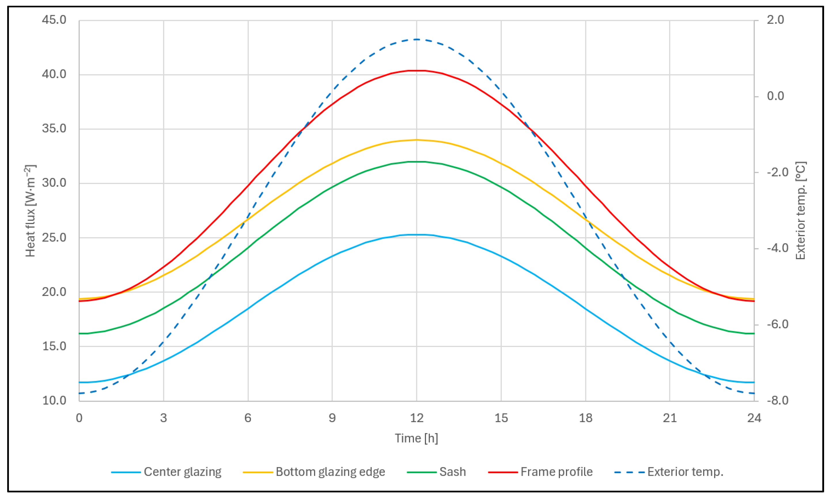
The results show that the highest local heat losses are concentrated in the lower part of the window assembly, especially in the lower frame profile, whereas the lowest values were recorded at the center of the glazing. Figure 4 also indicates a pronounced variation in heat flux density between different regions of the insulating glazing unit.

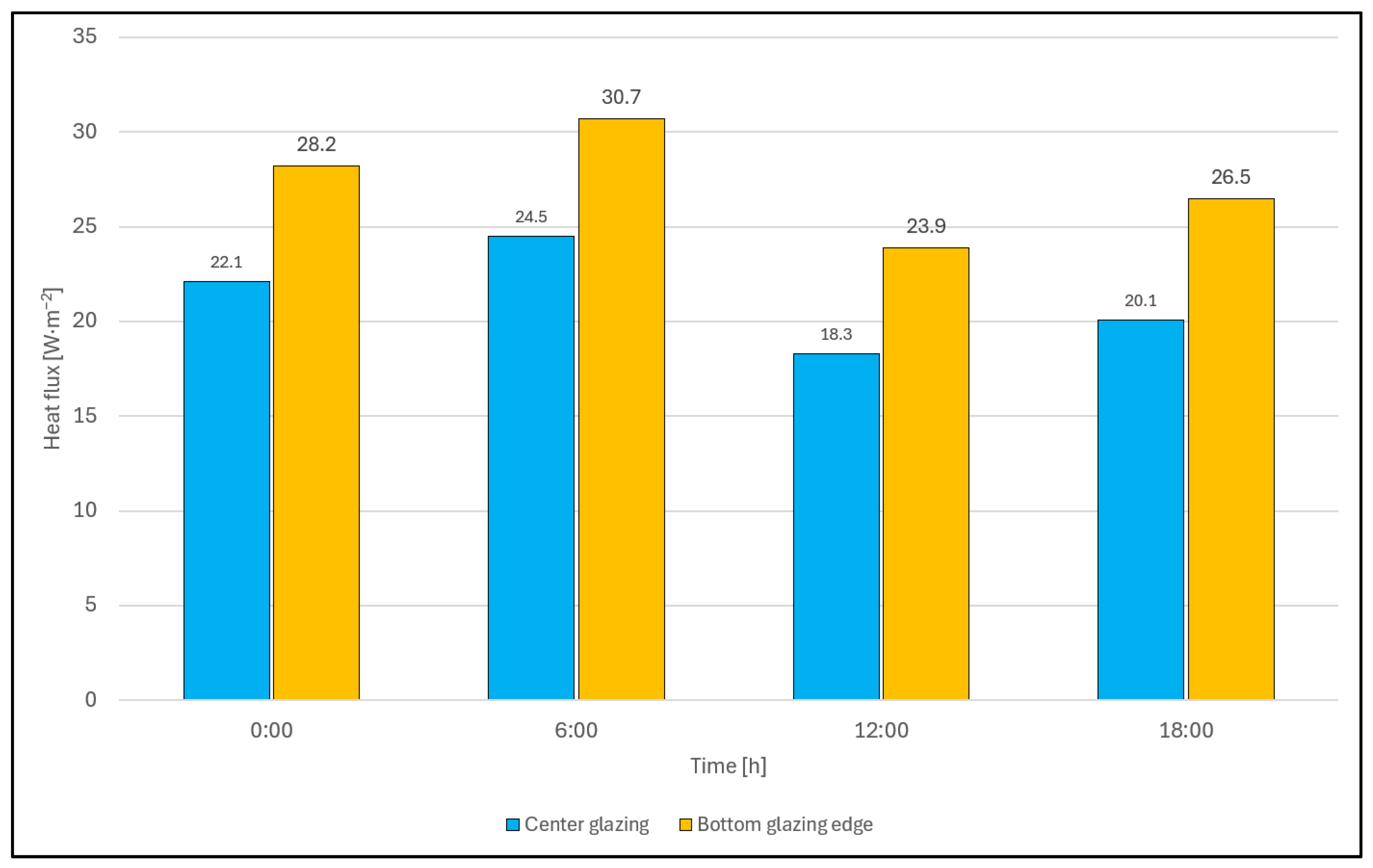
Figure 4 presents the temporal variation of heat flux density at several characteristic locations of the window assembly during a 24 h interval. For comparison purposes, the heat-flux curves represent time-aligned daily profiles. The profiles of the individual curves show that the heat fluxes are not constant but exhibit a pronounced time-dependent behavior closely related to changes in outdoor temperature and to the overall thermal regime of the surrounding environment. This dynamic response is typical of transparent building components with low thermal storage capacity, particularly glazing, which reacts rapidly to changes in boundary conditions [2,6].

The graph further indicates that the individual parts of the window exhibit different absolute values of heat flux density. The lowest values were recorded in the central glazing area, whereas higher values occurred in the glazing-edge regions and particularly in the lower part of the window assembly, namely at the lower frame profile. This variation suggests the nonuniform thermal behavior of the window and indicates the presence of linear thermal bridges in the edge regions, including the glazing edge, installation joint, and reveal. These findings are consistent with previous experimental studies [7,9], which reported increased heat fluxes in the glazing–frame contact zones.

The diurnal variation in heat flux density also reflects the cyclic nature of the outdoor boundary conditions. The highest heat flux values were observed during the night and early morning hours, when the indoor–outdoor temperature difference was greatest. In contrast, heat flux density decreased during the daytime as a result of increasing outdoor air temperature and possible solar gains. In a representative 24 h period without direct solar exposure, heat flux density decreased by approximately 20–25% between the morning maximum and the daytime minimum, further illustrating the sensitivity of the instantaneous heat flux to variations in the indoor–outdoor temperature difference. This trend is consistent with previous in situ studies of building envelope components, which demonstrated a strong relationship between the temperature difference and the magnitude of heat flux [4,32].

Another important observation is the relative stability of the differences between the individual measurement locations throughout the entire daily cycle. Although the absolute heat flux density values fluctuate over time, the ranking of the individual parts of the window assembly in terms of heat losses remains largely unchanged. This indicates that the identified critical zones are primarily governed by the structural design of the window rather than by instantaneous climatic conditions alone. This observation is consistent with the conclusions of previous research [1], which emphasized the need for spatially resolved assessment of window assemblies instead of relying solely on a single global U-value.

The curved profiles shown in Figure 4 underline the importance of long-term measurements. Short-term monitoring may fail to capture the full range of heat flux variability and may therefore lead to misleading conclusions regarding the thermal behavior of the window assembly. In contrast, long-term monitoring makes it possible to identify recurring patterns and to distinguish systematic effects from random fluctuations more reliably. This is consistent with the methodological considerations for in situ assessment of thermal performance reported in previous studies [1,2].

The results highlight the need to optimize the details in the glazing-edge regions and at the connection between the window frame and the building envelope. Such an approach enables a more detailed understanding of heat flux distribution and facilitates the identification of potential measures for reducing thermal losses [21,43].

3.2. Analysis of Local U-Values Under Quasi-Stationary Conditions

More stable weather conditions allowed a more accurate determination of the thermal transmittance. Several time intervals were used to calculate local U values under quasi-stationary conditions, the longest quasi-stationary time interval being from the evening of 18 January to the afternoon of 19 January. During this period, the outdoor air temperature remained quasi-stationary for more than 15 h, with an average value of 1.88 ± 0.28 °C.

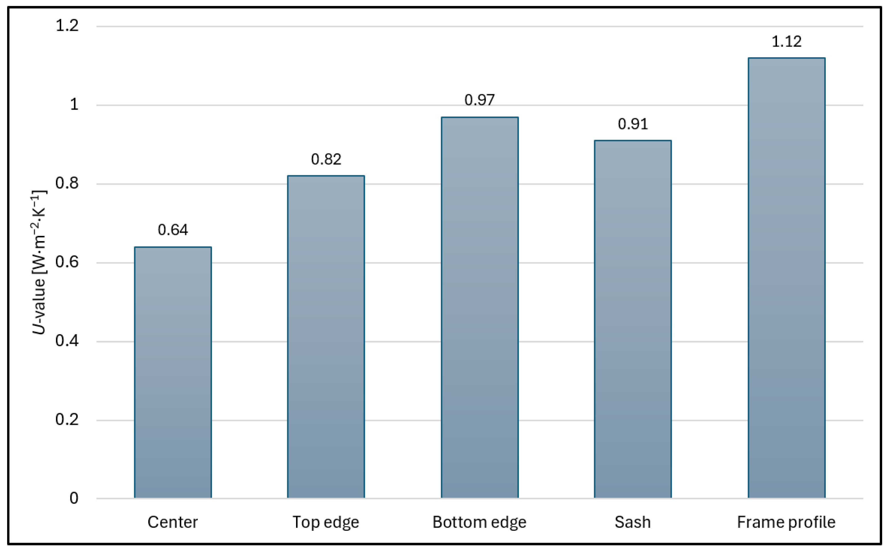
Figure 5 presents a comparison of the local thermal transmittance U for selected parts of the window assembly, including the center of the glazing, glazing-edge regions, sash, and lower frame profile, determined under quasi-stationary conditions. The results show substantial spatial variability in the calculated local U-values, exceeding 50% within the glazing itself. The lowest values were recorded in the central glazing area, whereas the highest values were observed in the frame components and lower frame profile.

The lowest local U-value was recorded at the center of the glazing (U = 0.64 W·m⁻²·K⁻¹), which is consistent with expectations and closely corresponds to the manufacturer-declared glazing value of U_g = 0.63 W·m⁻²·K⁻¹. This declared value refers to the homogeneous central part of the glazing under idealized conditions. Previous experimental and numerical studies [6,8] have confirmed that the center of glazing is the most representative area for assessing the thermal performance of insulating glass, as it is not influenced by edge effects associated with the installation of the glazing within the frame.

In contrast, the increased U-values observed in the glazing-edge regions highlight the importance of the linear thermal bridge at the glazing–frame interface. This phenomenon has been examined in detail in experimental studies [7,9], which showed that edge regions can exhibit heat losses several tens of percent higher than those recorded in the central glazing area. These increased values result from the combined effects of several factors, particularly the presence of the spacer bar, changes in material properties, and the more complex temperature field in this region.

A more pronounced increase in the local U-value was observed for the frame components, particularly the sash and the lower frame profile. This confirms that the window frame remains a critical component in terms of local heat losses, even when high-performance glazing is used. These findings are consistent with the studies [18,20], which showed that the thermal performance of window frames is strongly affected by their structural design, material composition, and internal configuration. Moreover, the actual local U values under in situ conditions may exceed the manufacturer-declared values, which are typically determined by using simplified procedures according to EN ISO 10077-1 [48] and EN ISO 10077-2 [49], particularly due to interactions with adjacent construction details.

Special attention should be paid to the lower frame profile of the window frame, which exhibited the highest local U-values. This suggests that this part of the assembly represents a significant source of local heat loss within the window construction. Similar findings have been reported in studies addressing window-to-wall connection details [21,26,27,28], where installation details and the position of the window within the reveal were shown to have a substantial effect on the resulting thermal bridges.

A sensitivity analysis was performed to evaluate whether the calculated local apparent U-values were affected by the selected duration of the quasi-stationary evaluation interval. Using the 6 h interval as the reference, shortening the evaluation period to 4 h resulted in a maximum difference of 2.20% in the calculated local apparent U-values, with a mean absolute difference of 0.84% across the four investigated locations. Extending the interval to 8 h resulted in an even smaller maximum difference of 1.02%, with a mean absolute difference of 0.80%. The largest individual difference was observed at the glazing edge for the 4 h interval (+2.20%). Importantly, the relative ranking of the investigated window regions remained unchanged for all three evaluation durations. Similarly, varying the heat-flux stability threshold from the reference 5% to 3% and 10% resulted in maximum differences of only 0.78% and 0.83%, respectively. The mean absolute differences associated with the threshold variation were approximately 0.50%. Importantly, the relative ranking of the investigated window regions remained unchanged in all cases. These results demonstrate that the calculated local apparent U-values and the principal conclusions regarding spatial differences in thermal performance are not materially sensitive to reasonable variations in either the selected stability threshold or the evaluation duration.

From a methodological point of view, Figure 5 confirms that relying on a single global U_w value may be insufficient for accurately characterizing the thermal behavior of a window assembly. Previous reviews and experimental studies [1,2] have emphasized the need for a more detailed assessment of individual window components, particularly in the context of in situ measurements.

These results confirm the importance of combining experimental and numerical methods, as this approach enables a more detailed understanding of heat flux distribution and supports the identification of potential measures for reducing thermal losses [43,44].

3.3. Analysis of Phase Shifts Within the Window Assembly

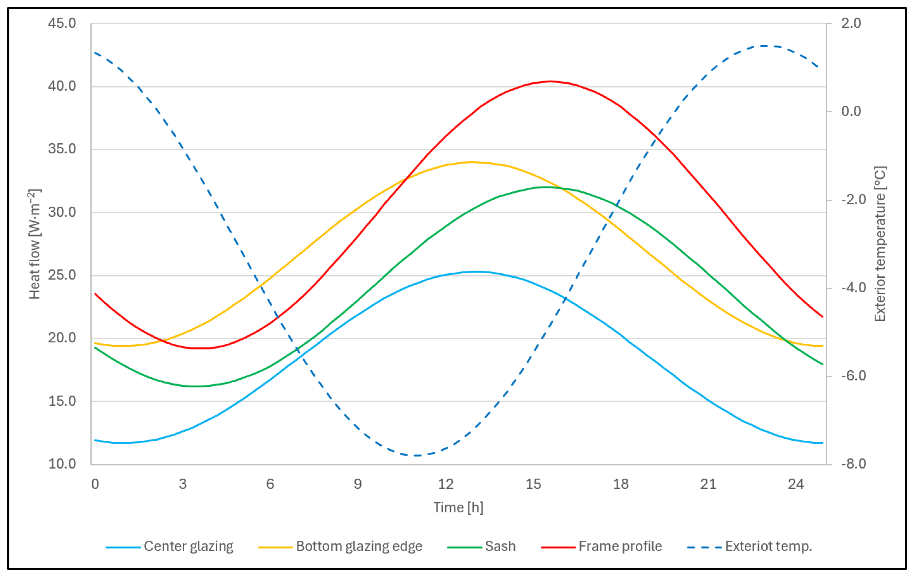
Time intervals characterized by pronounced dynamic changes in outdoor temperature and associated variations in heat flux density were selected to analyze the phase shifts in temperature response on the internal surface of the window assembly. The phase-shift analysis was performed independently for several daily measurement periods. The representative daily profiles shown in Figure 6 illustrate the characteristic dynamic response, whereas the reported phase-shift intervals summarize the range of delays observed across all analyzed days.

Table 3. Variation in measured heat flux density during the one selected measurement period. The values shown represent the arithmetic mean ± standard deviation (SD) of measurements in the analyzed time interval.

Measurement Location	qmin (W·m−2)	qmax (W·m−2)	Difference (W·m−2)
Center of glazing	15.2 ± 0.8	21.7 ± 1.3	≈6.5
Lower edge of glazing	20.4 ± 1.8	31.5 ± 3.1	≈11.1
Sash	18.9 ± 1.4	28.2 ± 2.1	≈9.3
Lower window frame profile	23.7 ± 1.9	33.3 ± 2.8	≈9.6

shows that the lower part of the glazing exhibited the highest variability in heat flux density.

Figure 6 illustrates the dynamic heat flux response in individual parts of the window assembly, with particular attention paid to the phase shift between the outdoor air temperature and the heat fluxes through the interior window construction. The phase shift was evaluated using cubic spline peak to peak curves for local values of temperature and heat flux. The analysis showed that the maximum heat flux values in the central glazing area and at the lower glazing edge occurred almost simultaneously, approximately 30–40 min after the minimum outdoor air temperature. The time shift between the two glazing-related profiles was negligible (≈0–10 min). In contrast, the heat flux profile measured on the window sash and lower frame profile exhibited a delay of approximately 90–120 min relative to maximum heat flux on glazing. These intervals represent the minimum-to-maximum phase shifts observed on different days, demonstrating that the differences in dynamic response between the glazing and frame components were repeatedly observed rather than being specific to a single selected period. The average time shift between the sash and the lower frame was less than 10 min. The temperature maximum was reached on the inner surface at almost the same time as the maximum heat flux (shift of 0–10 min.). These differences indicate the distinct dynamic thermal response of the individual structural components of the window assembly. The significant time lag in the response is primarily due to the sash and frame material (wood and aluminum cladding vs. glass and gas), thickness of locally measured layers and in the case of the frame, the connection to the sill and wall construction also plays a significant role. Cross-correlation analysis confirmed a significant difference between the dynamic response of the glazing and the frame components. The glazing was characterized by a delay generally in the range of 30–40 min. This behavior was independently confirmed by a second set of measurements, in which the median delay was in the same range. In contrast, significantly longer delays were obtained for the sash and the frame bottom profile. In five complete daily records, the median delay was 90 min for both components, while the average delays were about 105 ± 23 min for the sash and the frame bottom (mean ± SD across days). Although the exact delay varied between days, the cross-correlation analysis consistently demonstrated a significantly slower thermal response of the frame components than the glazing.

The synchronized heat flux profiles observed in the central glazing area and at the lower glazing edge indicate that these transparent regions are mainly governed by instantaneous boundary conditions, especially the indoor–outdoor temperature difference. This response is typical of elements with low thermal capacity, such as glass [6]. The similar dynamic behavior observed at the lower glazing edge suggests that, despite the presence of a thermal bridge at the glazing–sash interface, the temporal response of this region remains largely controlled by rapid heat exchange within the glazing system. This finding is consistent with experimental observations of heat flux distribution in window edge regions reported in [9]. In accordance with ISO 9869-1:2014 [46], for lightweight building components with low thermal capacity, defined as less than 20 kJ·m⁻²·K⁻¹, only night-time measurement data should be considered in order to minimize the influence of solar radiation. The recommended interval begins 1 h after sunset and ends at sunrise.

The substantially longer time lag observed for the sash and frame indicates a slower dynamic thermal response compared with the glazing. This difference may plausibly be associated with the greater thermal mass and heat-storage capacity of the frame assembly, together with its more complex geometry and multidimensional heat-transfer paths. However, the present measurements do not allow the individual contributions of these mechanisms to be separated, and the attribution to thermal storage should therefore be regarded as a physically plausible interpretation rather than a directly demonstrated causal relationship. This effect has been confirmed by numerical and experimental studies that emphasize the importance of thermal capacity and the internal structure of the frame in dynamic heat transfer [18,20]. The observed delay can therefore be interpreted as a consequence of heat accumulation in the frame and lower frame profile, followed by the delayed release of thermal energy.

The phase shift between the individual parts of the window assembly further indicates the transient nature of heat transfer under real conditions. Previous studies [1,2] have shown that in situ measurements can reveal dynamic phenomena that are not adequately captured by standard steady-state models. The presence of a phase shift indicates that the individual components of the assembly do not transfer heat simultaneously but respond with a certain time delay. This affects both instantaneous heat fluxes and the overall energy balance of the window assembly.

A physically plausible explanation for the slower response of the frame components is their greater effective thermal mass and heat-storage capacity compared with the glazing, combined with the more complex geometry and multidimensional heat-transfer paths within the frame assembly. Materials with greater thermal inertia generally respond more slowly to changes in boundary conditions. Nevertheless, thermal storage capacity was not independently measured or varied in the present experiment, and other factors, including frame geometry, local thermal bridges, and transient boundary conditions, may also contribute to the observed lag. Consequently, the present results demonstrate the difference in dynamic response but do not establish thermal storage capacity as its sole or direct cause. Similar conclusions have been reported in studies addressing the dynamic behavior of building components, e.g., [4], where different materials were shown to respond to temperature variations with different time delays.

From a practical point of view, this phenomenon has several important implications. First, it shows that instantaneous heat flux values do not necessarily represent the steady-state behavior of the window assembly, which is particularly important for U-value evaluation. Second, the observed phase shift may influence indoor thermal comfort, as different parts of the assembly respond to changes in outdoor boundary conditions with a time delay. Third, this finding underlines the importance of combining measurements with numerical simulations when analyzing the thermal behavior of construction details [43,44].

3.4. Influence of Temperature Difference on Local U-Value Determination

During the monitored period, a temporary warming event occurred. An 8 h interval was selected from this period, during which quasi-stationary conditions were observed, with an outdoor air temperature 8.86 ± 0.34 °C and an indoor air temperature 20.72 ± 0.33 °C. As a result of the smaller indoor–outdoor temperature difference, the recorded heat fluxes decreased. These data were used to evaluate the influence of the temperature difference during measurement on the calculated U-values.

Table 4. Average heat flux density ± SD and calculated U-values under low indoor–outdoor temperature difference conditions.

Measurement Location	q (W·m−2)	U (W·m−2·K−1)
Center of glazing	7.9 ± 0.8	≈0.66
Lower edge of glazing	11.7 ± 1.3	≈0.98
Sash	11.3 ± 1.2	≈0.95
Lower window frame profile	14.4 ± 1.3	≈1.21

summarizes the mean heat flux and local apparent U-values obtained during the selected 8 h low-ΔT quasi-stationary period, whereas Figure 7 is based on the broader set of individual measurements covering a range of indoor–outdoor temperature differences. Accordingly, the values in Table 4 correspond to one specific portion of the ΔT range represented in Figure 7 and are not expected to coincide with every point of the plotted curves. Table 4 values correspond approximately to the region around ΔT≈ 11.8 K in Figure 7.

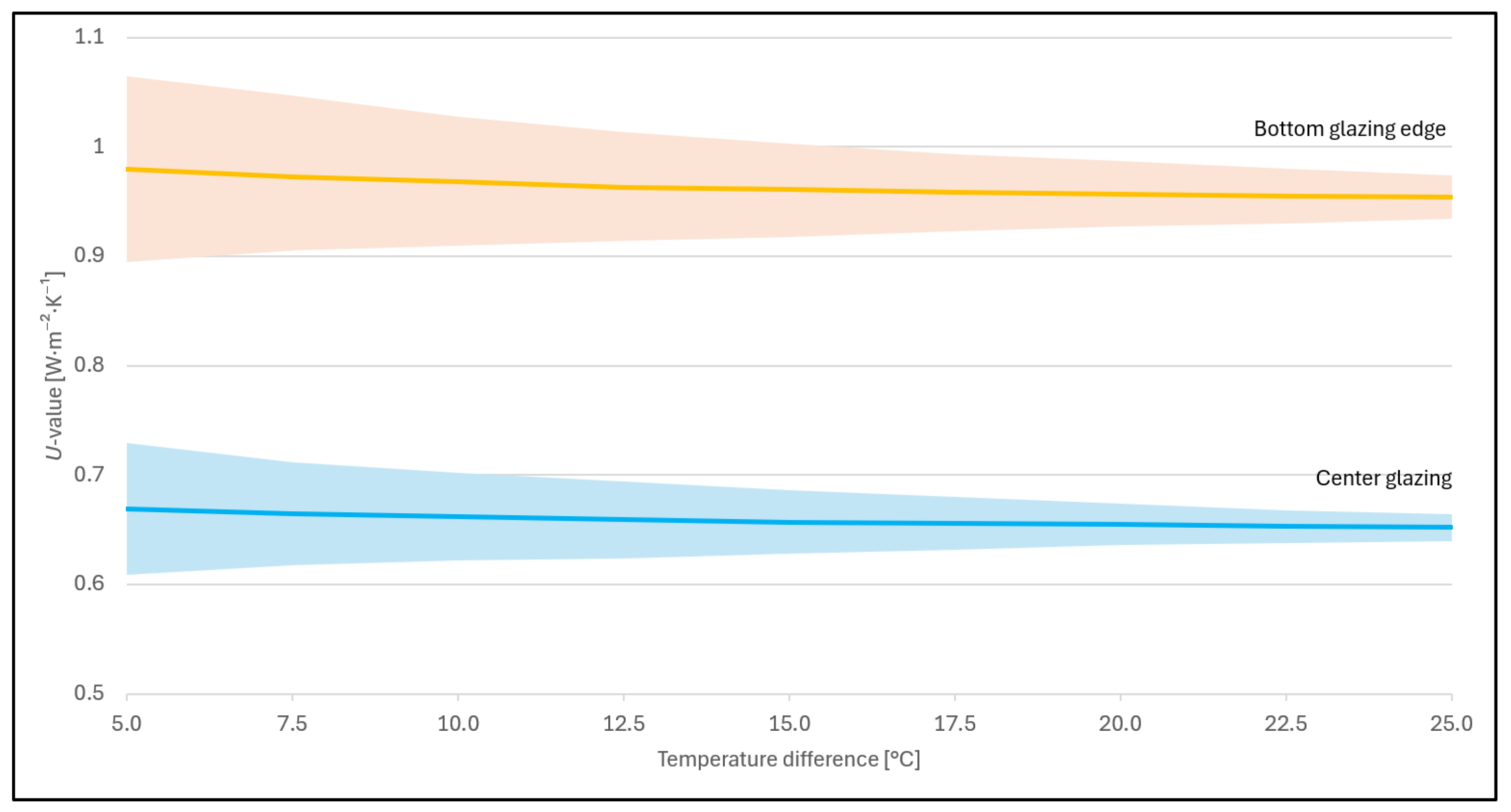
Figure 7 illustrates the dependence of the determined local thermal transmittance U on the magnitude of the temperature difference ΔT between the indoor and outdoor environments. The profiles show that the calculated local U-value is not stable but exhibits a certain degree of variability depending on the magnitude of the temperature gradient, with this effect being more pronounced at lower ΔT values. Similar behavior has also been identified in experimental studies [1,2] focused on in situ U-value measurements, which highlight the sensitivity of the results to boundary conditions and measurement quality. From the perspective of thermal transmittance determination, the results obtained during this period were less accurate, as the smaller temperature difference increased the relative error of the calculation. This issue is also recognized in in situ measurement methodologies [46].

The uncertainty bands shown in Figure 7 were calculated by propagating the instrumental uncertainties of the heat-flux and temperature measurements through U = q/ΔT using Equation (2). For each ΔT interval, the uncertainty was calculated at the corresponding mean heat-flux and temperature-difference values. The shaded regions therefore represent the propagated instrumental uncertainty of the calculated local apparent U-values and not the standard deviation of the measured data. At small temperature differences, approximately up to 5–10 K, the uncertainty of the thermal transmittance calculation increases. This effect follows directly from the definition U = q/ΔT, where a low denominator value leads to an increase in the relative error. As reported in studies [32,33], the accuracy of the heat flux method decreases considerably at low temperature differences, since even small errors in heat flux or temperature measurements can result in significant deviations in the calculated local U-value. In the graph, this effect is reflected by a larger scatter of values and their reduced stability.

As the temperature difference increases, particularly above approximately 15 K, the calculated local U-values become more stable and converge toward the expected value. This trend is consistent with previous in situ studies, which have shown that a higher temperature gradient improves the reliability of thermal transmittance determination. The improvement in accuracy at higher ΔT values is related to an increased signal-to-noise ratio, which is a key factor in the experimental assessment of thermal performance parameters [4]. The stabilization of the curves also indicates that the measurement approaches quasi-stationary conditions, which are required for reliable evaluation according to in situ measurement procedures [1,46].

Figure 8 also shows that the difference between the central glazing area and the edge region is maintained over the entire range of temperature differences. This indicates that the identified differences are not merely the result of measurement uncertainty but reflect the actual physical behavior of the window assembly. The influence of edge regions and linear thermal bridges has also been documented in studies focused on heat flux distribution in windows [7,9], which reported a systematic increase in heat losses outside the central glazing area.

The results confirm the recommendations in technical standards and the scientific literature that the indoor–outdoor temperature difference during measurement should be sufficiently large and stable. For example, the review study [1] states that an insufficient temperature difference is one of the main sources of uncertainty in the experimental determination of U-values. Similarly, study [39] emphasizes the importance of measurement sensitivity analysis, showing that the accuracy of the results is strongly affected by the magnitude of ΔT and by fluctuations in boundary conditions.

Measurements should preferably be conducted during the winter period, when higher indoor–outdoor temperature differences are naturally achieved. In addition, time intervals characterized by minimal fluctuations in outdoor boundary conditions should be selected. Alternatively, the heat flux method may be combined with infrared thermography, which allows local deviations in the temperature field to be identified more effectively and provides additional support for the interpretation of the results [46,50].

3.5. Synthesis of Results—Local Thermal Transmittance Values

Based on the processing of all measurements, thermal transmittance values were determined for the individual parts of the window assembly.

The summarized results (

Table 5. Summary of calculated local thermal transmittance values for individual parts of the window assembly.

Window Component	Umin (W·m−2·K−1)	Umax (W·m−2·K−1)	Uaverage (W·m−2·K−1)
Center of glazing	0.63	0.70	≈0.66
Lower edge of glazing	0.80	1.10	≈0.95
Sash	0.90	1.40	≈1.10
Lower window frame profile	1.10	1.60	≈1.25

) of the experimental measurements confirm that the thermal performance of the window assembly is spatially heterogeneous and depends on the specific location within the window component. The local apparent U-values measured at the center of the glazing ranged from approximately 0.63 to 0.70 W·m⁻²·K⁻¹. Although the locally measured quantity is not strictly equivalent to the standardized value, this range is consistent with the manufacturer-declared U_g value of 0.63 W·m⁻²·K⁻¹ and therefore provides a useful reference for the plausibility of the in situ measurements. This difference confirms that declared parameters represent ideal laboratory conditions and primarily refer to homogeneous parts of the construction [6,8].

In the glazing-edge regions, local U-values in the range of U = 0.8–1.1 W·m⁻²·K⁻¹ were determined, representing a significant increase compared with the central glazing area. This result is consistent with experimental studies highlighting the importance of linear thermal bridges in this region [7,9]. Even more pronounced deviations were recorded for the lower frame profile, where the local values reached up to 1.2–1.5 W·m⁻²·K⁻¹. This difference can be attributed not only to the methodology used to determine the thermal transmittance of window frames, and to the material properties of the frame, but also to the influence of the connection to the building structure and installation details, which represent significant sources of local heat loss under real operating conditions [20,21].

From the perspective of the overall assessment, it can be stated that the experimentally determined values locally exceed the declared overall window thermal transmittance, U_w = 0.67 W·m⁻²·K⁻¹, specified for a window size of 1230 × 1480 mm, particularly in critical details. This finding confirms the conclusions of review studies [1,2] that highlight the discrepancy between laboratory-determined, and in situ measured thermal performance parameters.

The synthesis of the results indicates that for the investigated window assembly the global U_w value may not sufficiently represent the actual thermal behavior of the window assembly, as it does not account for local extremes in heat fluxes. This aspect is particularly important from the perspective of energy balance and the assessment of condensation risk, which is governed by the coldest locations within the construction. The reported local U-values represent point-specific heat transfer conditions obtained from HFM measurements and should not be interpreted as the overall window thermal transmittance U_w. The comparison is intended to highlight the spatial variability of thermal performance and the presence of local thermal bridges rather than to replace the standardized area-weighted U_w value.

3.6. Analysis of Surface Temperature Fields of the Window Assembly

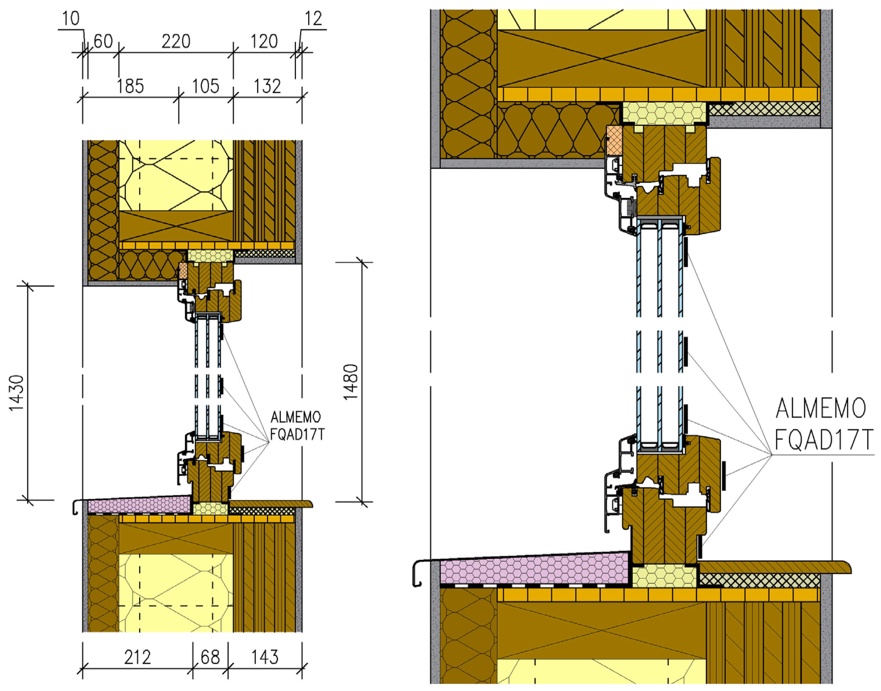
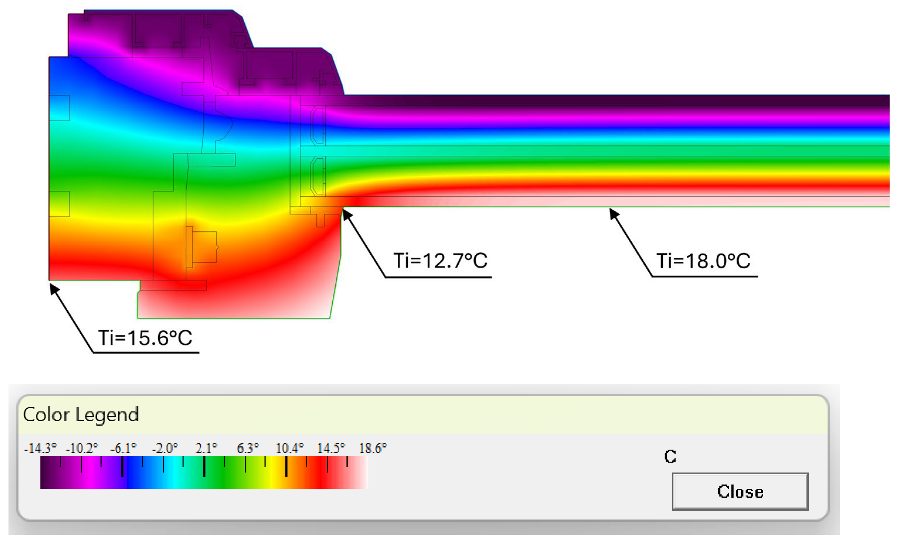
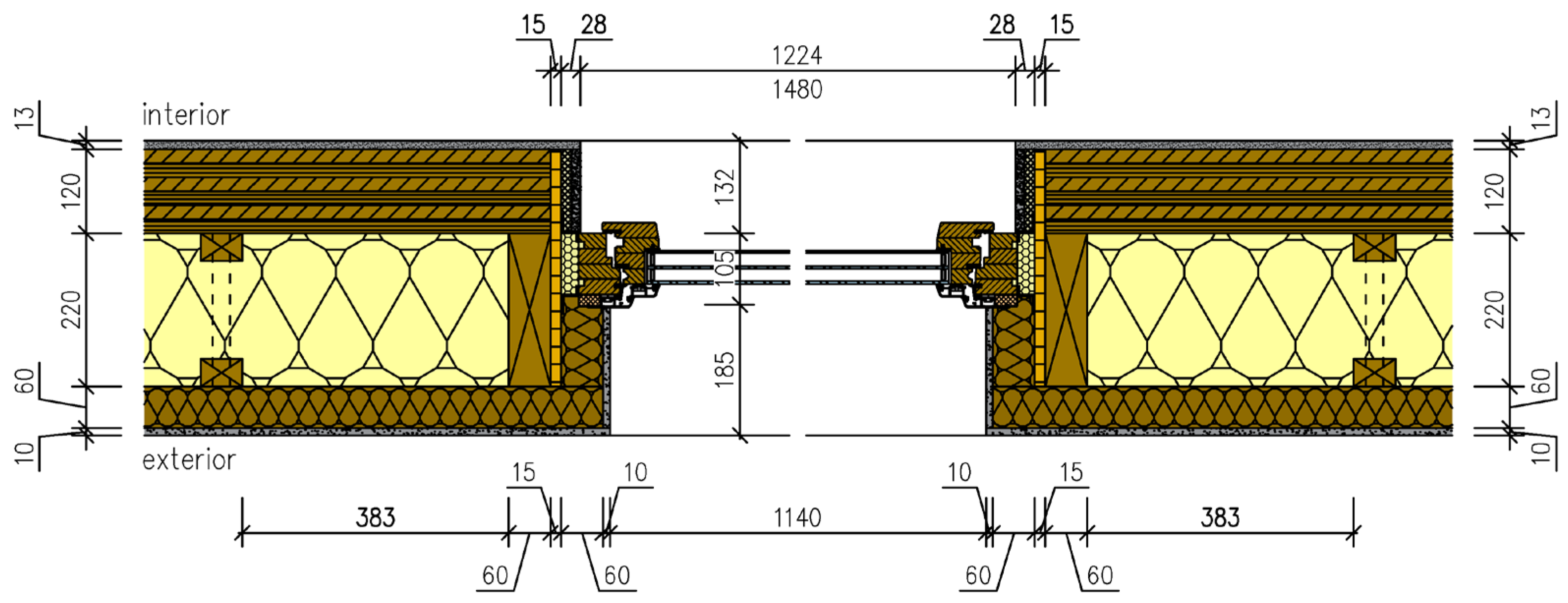
As a supplement to the in situ measurements, a two-dimensional heat transfer analysis was performed for the investigated window assembly and its installation detail in the research building. The analysis of the spatial surface temperature fields of the MINTAL Classic wood–aluminum window profile (Figure 9), conducted using THERM 7.6 software (Lawrence Berkeley National Laboratory), confirmed that the window assembly meets the requirements of STN 73 0540-2:2019 [45] for the minimum internal surface temperature. The properties of the materials used in the model are listed in

Table 6. Thermophysical Properties of Materials Used in the THERM Numerical Model.

Material	Thermal Conductivity λ (W·m−1·K−1)	Emissivity ε (-)
Softwood	0.130	0.85–0.95
Anodized aluminum alloy	200	0.77
EPDM gasket	0.25	0.90–0.95
Glass (plate or float)	1.00	0.84
Argon	0.017	0.00
Swisspacer spacer bar	0.135	0.93–0.95
Polypropylene	0.22	0.97
Butyl sealant	0.24	0.90–0.97
Galvanized carbon steel	50	0.46
Polyurethane (PUR) foam	0.030	0.90–0.95
Extruded polystyrene (XPS)	0.034	0.84–0.95
Mineral plaster	0.91	0.90–0.95
Wood-fiber insulation	0.043	0.90–0.95
OSB	0.15	0.90–0.95
Gypsum plasterboard (Type A)	0.25	0.90
Frame cavity NFRC 100	0.1394	-
Frame cavity Slightly Ventilated NFRC 100	0.1281	-

.

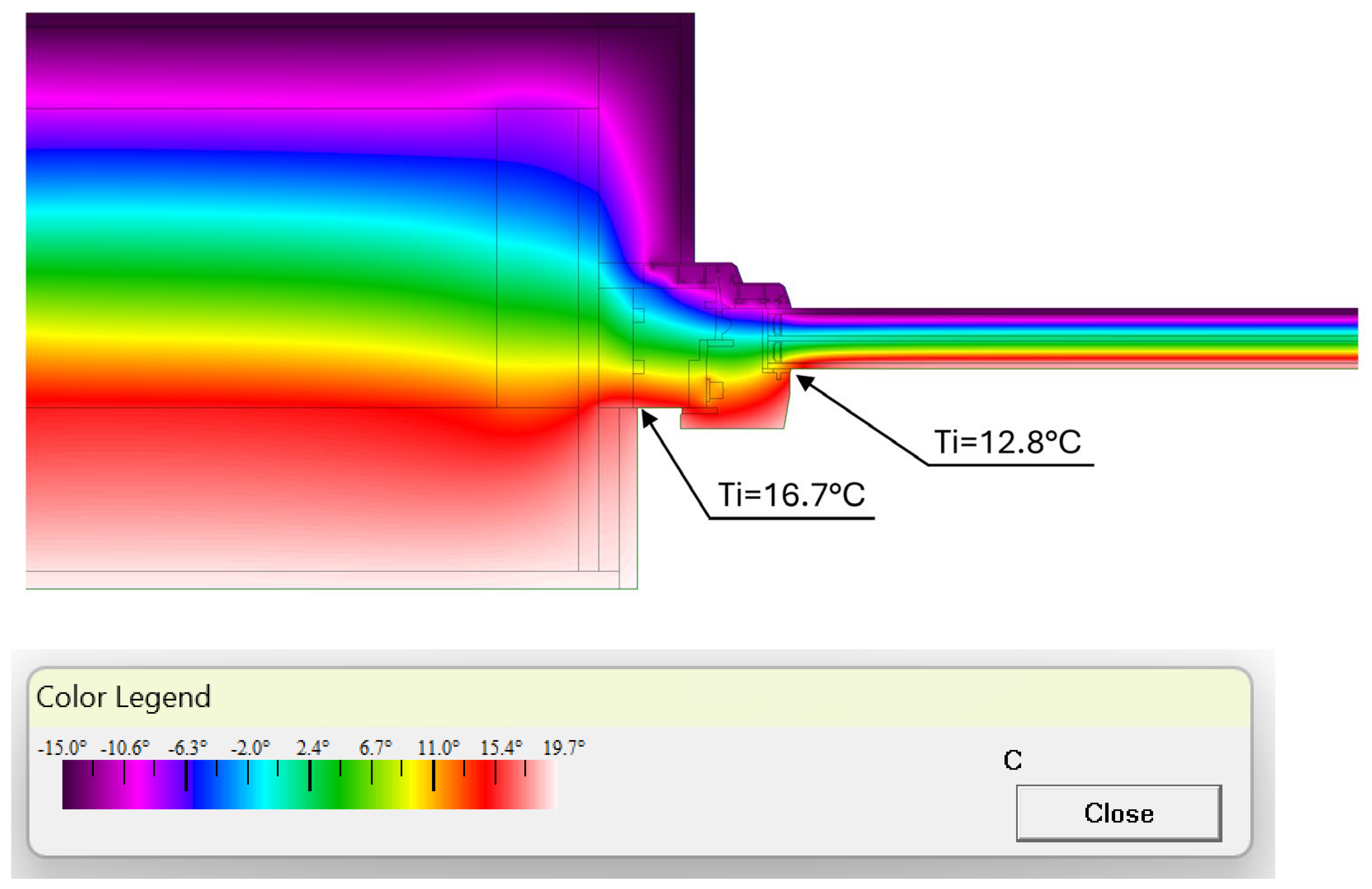
The minimum internal surface temperature in the reveal, corresponding to the window–external wall junction, remains safely above the required limit temperature of 12.8 °C (Figure 10). The linear thermal transmittance of the lateral window installation detail, ψ_i, was determined to be 0.0045 W·m⁻¹·K⁻¹. This suggests an appropriate insulation design and a sufficient exterior overlap of the thermal insulation onto the window frame.

The objective of the THERM analysis was to support the interpretation of experimentally measured heat-flux and temperature distributions and to identify critical thermal bridge regions within the investigated window assembly. The finite-element mesh was generated using the THERM automatic meshing procedure with mesh parameter 9, which corresponds to the finest level of mesh discretization for the given detail. Geometrical simplifications were intentionally minimized and were limited to selected secondary features of the external aluminum cladding profile and sealing gaskets. Previous studies have shown that progressive mesh refinement beyond the convergence region generally results in only marginal improvements in solution accuracy while substantially increasing computational effort [51].

A mesh-sensitivity analysis was performed to verify that the calculated surface temperatures were not materially affected by the finite-element discretization. Five successive mesh settings (5–9) were evaluated, and the internal surface temperatures were compared at four representative locations: the center of the glazing, glazing edge, sash, and window frame. For mesh settings 5–8, the calculated temperatures were identical within the reported numerical resolution of 0.1 °C, yielding 18.0, 15.5, 17.0, and 15.7 °C at the respective locations. Further mesh refinement (mesh setting 9) produced no change at the center or edge of the glazing and only minor differences of −0.1 K at the sash and +0.2 K at the frame. The maximum difference between the two finest evaluated mesh settings was therefore 0.2 K. These results indicate negligible sensitivity of the calculated surface temperatures to further mesh refinement and confirm that the adopted discretization was sufficiently refined for the purposes of the present analysis.

The validation was based on 32 measurement records comprising 128 measured–predicted surface-temperature pairs at four representative locations. Across the complete dataset, the model yielded an RMSE of 1.80 K, a mean bias error (MBE; predicted minus measured) of +1.55 K, and a maximum absolute deviation of 4.01 K. The coefficient of determination between measured and predicted temperatures was R² = 0.731. The positive MBE indicates that the numerical model systematically overpredicted the measured internal surface temperatures.

Table 7. Statistical evaluation of agreement between measured and THERM-predicted surface temperatures at the investigated window locations.

Measurement Location	RMSE (K)	MBE (K)	Max. Deviation (K)	R2 (-)
Center of glazing	1.11	+1.09	1.48	0.934
Lower edge of glazing	3.06	+3.00	4.01	0.993
Sash	1.30	+1.29	1.50	0.977
Lower window frame profile	0.86	+0.84	1.18	0.992

shows that the agreement was strongly location-dependent. A substantially larger discrepancy was observed at the lower glazing edge, where the RMSE reached 3.06 K and the maximum deviation was 4.01 K. Thus, the overall model error was dominated by the glazing-edge region, whereas considerably closer agreement was obtained at the other three locations.

The larger discrepancy at the lower glazing edge is likely related to the strongly two-dimensional heat-transfer conditions in this region, including the spacer, glazing–frame junction, and local geometric details. In addition, the experimental temperature represents the specific thermocouple position, whereas the numerical result is sensitive to the exact location at which the surface temperature is extracted from the model. Consequently, small differences in the experimental and numerical evaluation positions may produce considerably larger temperature differences in this region than in the relatively homogeneous center-of-glazing area.

3.7. Limitations

The present study provides a detailed long-term in situ assessment of the thermal performance of a single wood–aluminum window installed in a real timber building under winter climatic conditions. Nevertheless, several limitations should be acknowledged. First, the measurements were performed on one window type installed in a specific wall configuration; therefore, the results should not be generalized to all window systems or installation details without further verification. Second, the analysis was conducted during the heating season only, when sufficiently large indoor–outdoor temperature differences allowed reliable application of the heat flow meter method. Consequently, the influence of summer boundary conditions, increased solar gains, and reverse heat flow was not investigated. The obtained values should therefore not be directly extrapolated to summer conditions, particularly in hot climates, where reduced or reversed temperature gradients and solar radiation may significantly affect the measured heat flux. A dedicated summer investigation accounting for solar gains and transient boundary conditions would be required to characterize the thermal performance of the window under cooling-dominated conditions. Furthermore, although the measurements covered a relatively long monitoring period, short-term fluctuations caused by wind, solar radiation, and transient environmental conditions may have locally affected the measured heat fluxes despite the selection of quasi-stationary evaluation intervals. Future research should include different window types, façade orientations, and climatic conditions, together with coupled experimental–numerical analyses aimed at broader validation of the proposed methodology.

A limitation of the present study is that the measurements were performed on a single wood–aluminum window assembly at one Central European location. Therefore, the reported local apparent U-values are specific to the investigated construction and boundary conditions.

3.8. Measurement Uncertainty and Methodological Sources of Error

The uncertainty of the calculated thermal transmittance is primarily associated with the accuracy of the heat flux sensors, temperature measurements, sensor installation, and the transient nature of the boundary conditions during in situ monitoring. To minimize these effects, all heat flux sensors were installed using thermal paste to reduce contact resistance, and the thermal transmittance was evaluated preferentially during quasi-stationary periods characterized by stable indoor–outdoor temperature differences. Because the calculated local U-value is obtained from the ratio between heat flux density and temperature difference, the relative uncertainty increases as the temperature difference decreases. For this reason, the results obtained under larger temperature differences (approximately ΔT > 15 K) are considered the most reliable and are in agreement with the recommendations of ISO 9869-1.

The propagated uncertainty calculated from the instrumental contributions represents only the uncertainty associated with heat-flux and temperature sensing. The total uncertainty of an in situ local apparent U-value is necessarily larger because additional effects arise from sensor installation and environmental conditions. Sensor positioning is particularly relevant in the glazing-edge and frame regions, where steep lateral temperature and heat-flux gradients may occur; therefore, small changes in sensor location may lead to physically different local values rather than merely random measurement errors. Similarly, imperfect sensor–surface contact can alter the measured heat flux, although this effect was reduced by the application of thermal paste. Radiative exchange and solar exposure can also perturb the surface heat balance, which was one reason for preferentially evaluating quasi-stationary and night-time periods.

Boundary-condition and data-processing effects were reduced by long-term monitoring and by selecting stable intervals. The sensitivity analysis demonstrated that changing the evaluation duration between 4 and 8 h affected the local apparent U-values by no more than 2.20%, while varying the stability threshold between 3% and 10% resulted in changes below 0.83%. Thus, the data-processing choices constitute a relatively small contribution compared with the instrumental and location-dependent sources of uncertainty. Nevertheless, because several installation- and environment-related contributions could not be independently quantified from the available measurements, the propagated uncertainty reported in this study should be regarded as an instrumental uncertainty estimate rather than a complete uncertainty bound for the in situ method.

4. Conclusions

This study presented an experimental assessment of the thermal performance of a wood–aluminum window installed in a real timber building under actual climatic conditions, with particular emphasis on long-term in situ measurements of heat flux and temperature variations. The results confirmed the spatially heterogeneous thermal behavior of the window assembly, as individual window components exhibited different thermal transmittance values and distinct dynamic responses. The central glazing area showed values close to the manufacturer-declared parameters, whereas the glazing-edge regions and frame components exhibited substantially higher local heat losses due to the presence of linear thermal bridges.

The analysis of the time-dependent heat flux profiles revealed a pronounced diurnal cycle, governed primarily by the indoor–outdoor temperature difference. The frame components exhibited a substantially slower dynamic response than the glazing. Cross-correlation analysis indicated characteristic lags of approximately 90–120 min for the sash and lower frame, compared with the glazing. The greater thermal inertia of the frame assembly provides a physically plausible explanation for this behavior; however, the present measurements do not isolate thermal storage from other contributing effects, such as geometry and multidimensional heat transfer.

The comparison between the experimental results and the manufacturer-declared parameters showed that, under real operating conditions, local apparent U-values may be substantially higher than the declared global thermal transmittance of the entire window assembly. This finding indicates the limitations of assessing window performance using a single global value and highlights the need for a detailed, spatially resolved evaluation approach. The findings are relevant not only for research purposes but also for the design of nearly zero-energy buildings and the validation of numerical models. They also underline the importance of experimentally verifying thermal performance parameters under real conditions.