


Abstract
Construction sites are beginning to deploy material transport robots to relieve labor constraints; however, planning and validating robot operations within complex, evolving building layouts remain difficult. This study proposes a BIM-enabled simulation framework that connects building information to enable an objective pre-deployment evaluation. The method extracts navigable spaces, delivery points and material quantities from BIM, formulates dispatching as a capacity-constrained vehicle routing problem, and couples it with an A* algorithm for pathfinding. A greedy next-stop decision rule with a tunable correction factor governs whether the robot continues visiting additional stops or returns to the staging area. The experimental results show a more than 20% improvement in the travel efficiency of the robot compared with conventional algorithms. These results conclude that the framework offers a practical tool for what-if analysis and data-driven planning of robotized construction logistics and is readily extensible to diverse materials and project types.
1. Introduction
The International Labour Organization estimates that approximately 3 million people worldwide die each year from work-related accidents and diseases. In particular, the construction industry is identified as a high-risk sector, with a fatal accident risk three to four times higher than the industrial average [1,2]. Furthermore, over the past 20 years, the average annual growth rate of labor productivity in the global construction industry has been about 1%, which is significantly lower than that of the world economy (2.8%) and the manufacturing sector (3.6%) [3]. The construction industry has traditionally been characterized by its labor-intensive nature, resulting in high safety risks, chronic labor shortages, and low productivity [4,5]. Repetitive and strenuous tasks, such as material handling, lead to safety concerns for workers, while the decline in skilled labor is a major factor contributing to increased project costs and diminished quality [5,6,7,8,9]. The effectiveness of robotic technology has already been proven in the manufacturing and logistics sectors as a solution to these challenges [10,11,12]. The introduction of material-transporting robots at construction sites is expected to serve as an effective solution for enhancing worker safety and optimizing overall logistics flow.
Despite the potential benefits of introducing material transport robots, the complex and dynamic environments of actual construction sites create several technical limitations for robot operation. The site is filled with constantly changing obstacles, uneven ground, and harsh environmental conditions, such as dust [13,14,15]. Consequently, the Simultaneous Localization and Mapping (SLAM) system may experience errors in map creation and position tracking, hindering the smooth autonomous movement of robots [15]. In dusty environments, the sensor performance may deteriorate, forcing the SLAM system to perform more calculations to build an accurate map, thereby increasing the robot’s power consumption [16,17]. Furthermore, limited battery capacity restricts the robot’s continuous operation time, and when transporting heavy materials, leading to inefficiency owing to frequent recharging [18].
In addition, various issues must be addressed when operating material-transport robots. To enhance the efficiency of robot operations, it is necessary to optimize several variables, such as route planning for multiple stops, different types and quantities of materials required at each stop and loading and unloading of materials. In robot operations, the Vehicle Routing Problem (VRP) must be solved to assign and schedule missions efficiently, encompassing variants such as the Capacitated VRP (CVRP), VRP with Time Windows (VRPTW), Pickup and Delivery Problem (PD) and its time-window version (PDPTW), Multi-Depot VRP (MDVRP), Heterogeneous VRP (HVRP), and Split-Delivery VRP (SDVRP) [19,20]. In this study, we aim to solve the CVRP, focusing on it among the various VRPs.
To overcome these limitations of robot operation and verify efficiency in real-world settings in advance, simulation is essential. In particular, simulations based on Building Information Modeling (BIM) data offer the significant advantage of integrating actual site spatial information (such as walls and pathways), material information (such as quantity and weight), and robot specifications (such as speed and loading capacity) to create a realistic environment [21,22].
This study proposes a BIM-based simulation methodology for planning material transport robot operation. In particular, we developed an efficiency-driven algorithm to address the CVRP, reflecting the robot’s maximum load capacity and the site’s material demand. The proposed algorithm was developed by combining the A* and greedy algorithms to enhance the transport efficiency of the robot. The proposed algorithm was validated through a case study of a studio apartment project, and its practical effectiveness in robot operation was demonstrated by comparing and analyzing the performance of the simple sequential transport method and the proposed optimization algorithm.
2. Literature Review
Construction materials account for about 60% of the total project costs, and among these, shipping costs are classified as non-value-added activities, comprising 30% to 75% of the total material manufacturing expenses [6]. Furthermore, due to moving machinery, heavy equipment, and unpredictable working conditions at construction sites, transporting materials inherently involves various safety hazards [20]. Material transportation increases the risk of work-related musculoskeletal disorders (WMSDs) and can lead to injuries [7,8]. Additionally, the shortage of skilled labor and the transition to an aging society are becoming serious problems in the construction industry, forming a complex vicious cycle involving cost increases from rising wages, decreased construction productivity, and a higher likelihood of accidents [9,23,24]. As a solution to these multi-faceted problems, the introduction of robots for material transportation is being considered.
Automated Guided Vehicles (AGVs) and Autonomous Mobile Robots (AMRs) are being developed and applied in many industries. AGVs are mainly used for transporting heavy loads between fixed points. They move by following predefined routes along physical markers (e.g., magnetic tapes and QR codes) or virtual paths [11,12,25,26]. AGVs are limited to specific paths and have low flexibility; therefore, they are most effective in defined and controlled environments, such as large warehouses or fixed production lines [11,12,25].
In contrast, AMRs utilize advanced sensor technologies such as SLAM, 3D LiDAR, and cameras, as well as artificial intelligence, to navigate paths in complex environments with human-like intuition [26,27,28]. AMRs can scan their environment and make independent decisions to perform complex tasks without additional infrastructure. They can also detect and avoid obstacles and replan their routes in real time [28,29,30].
In the manufacturing and logistics industries, there have been numerous successful cases in which robotic technology has dramatically improved efficiency, safety, and sustainability by automating repetitive and labor-intensive tasks [31,32]. In the logistics industry, robots primarily perform transport tasks between fixed points and are sometimes limited to simple tasks, such as parcel delivery or material movement [11]. In warehouse automation, robots play a key role in maximizing efficiency and reducing errors by performing tasks such as picking, sorting, moving, storing, and retrieving items [12,28,30,33]. Boston Dynamics’ Stretch robot automates case handling in warehouses, accelerating container unloading to improve safety and throughput [34]. Teradyne’s AMRs can handle payloads from 250 kg to 1350 kg and include a pallet jack AMR for the autonomous movement of pallets [30]. Oceaneering Mobile Robotics (OMR) provides solutions that automate a range of logistics and manufacturing tasks, from lightweight to heavy-duty load handling, using navigation systems that require no additional infrastructure [35].
Based on these successful cases, various types of robotic technologies have been developed and tested to transport material at construction sites. However, due to the unpredictable and ever-changing nature of construction environments, AMRs and AGVs face several inherent operational limitations. Construction sites, with numerous obstacles such as temporary structures, equipment, materials, and piles of dirt, present particularly challenging environments for robots to navigate [13,14]. Construction site robots must also handle large components, function under adverse weather conditions, and withstand continuous exposure to dust and debris [26].
In addition to site environments, power consumption is the most important factor in operating a robot. The batteries used in modern robots mainly utilize lithium-ion technology, which offers a high energy density, and their capacity and operating time vary significantly depending on the robot model and its intended use. SLAM algorithms are inherently computationally intensive, and if not optimized, can consume excessive power, causing the battery to deplete rapidly. LiDAR (Light and Distance Detection) is considered the most essential and suitable class of sensors for detecting objects even in dusty environments [15,36]. High-performance sensors such as LiDAR require a certain amount of power consumption to detect its surroundings [16]. In particular, dusty environments impede sensor perception, forcing the SLAM system to perform more computations to determine its location and construct an accurate map. Such environments require robots to engage in constant dynamic replanning, a process that consumes a significant amount of battery life for the robot. Ultimately, this leads to shortened mission times and a vicious cycle in which the robot must return to the charging dock more frequently.
Boston Dynamics’ Spot, with a 564 Wh battery, offers about 90 min of operation under normal conditions [34]. In contrast, Agility Robotics’ humanoid robot Digit can operate for up to 4 h with its improved battery, while Figure AI’s F.03 is reported to run for up to 5 h at maximum performance because of its large 2.3 kWh battery [37,38]. However, these operating times are insufficient to cover large worksites, and depending on the environment and conditions of the construction sites, the operating time is expected to decrease significantly. In the case of material transportation robots, the payload (carrying capacity) of the robot is also related to battery consumption. The heavier the load carried by the robot, the faster the battery is depleted. Additionally, the energy consumption of the robot varied depending on the route [39,40]. This implies that complex tasks, such as lifting, manipulation, and dynamic movement, consume significant amounts of power. For example, with the MiR250, although it is said to be capable of operating for 17 h without carrying a load, in actual operation (with payload, inclines, repeated stops/starts, and increased friction due to dust), it is common to conservatively estimate a reduction of up to 40% [41].
In the construction field, extensive research has been conducted on simulating and optimizing the work of monitoring robots, such as Boston Dynamics’ SPOT, to scan construction sites. Frías et al. (2019) [42] demonstrated that scanning and route planning in a virtual space based on BIM prior to construction can improve the accuracy of quality control and the predictability of site operations. Additionally, Park et al. (2023) [43] showed that by simulating optimal scanning positions and routes through the integration of spatial information automatically extracted from BIM models and the operational characteristics of the robot platform, the scanning efficiency in actual construction sites can be significantly increased. This suggests that path planning utilizing BIM models goes beyond simple data integration, presenting the potential for advancements in robot operation stability and process management based on automation.
In the case of material transportation robots discussed in this study, simulations must consider not only simple movement but also more variables, such as the weight and size of materials by type, locations and times for loading and unloading operations, and more. Therefore, this study proposes a simulation framework for the path planning and operation of autonomous material-transport robots in a BIM environment. In particular, an algorithm was designed to comprehensively perform visibility analysis, obstacle avoidance, and optimal path calculation using the spatial information of the BIM-based construction environment. The first advantage of BIM in this context is its ability to simultaneously provide spatial information, including floor geometry, wall configurations, and accessible pathways. In addition, its quantity takeoff function enables the automatic extraction of material demand directly from the design model, which can then serve as input to a capacity-constrained routing formulation. While multi-robot coordination and routing strategies have been widely explored in robotics and traffic-related research [44,45], limited attention has been given to integrating architectural spatial data and construction material logistics information within a BIM-driven planning environment. Most prior studies focus on navigation efficiency or congestion modeling in abstract or road-based networks rather than construction-specific workflows grounded in building design data. The proposed framework addresses this gap by embedding BIM-derived geometry and material demand directly into robot deployment and transport sequence planning.
To reduce the energy consumption of robots, as described above, active research is underway on the software side to optimize robot movement and task routes. Some studies claim that this can result in nearly a 30% improvement in efficiency, indicating significant potential for improving battery life and operating time by making robot motion more efficient. Simultaneously, there is a growing emphasis on the need for preliminary path simulations and repeatable task planning verification processes in virtual environments to ensure efficient robot movement and task execution.
3. Methodology
3.1. BIM-Enabled Simulation Process
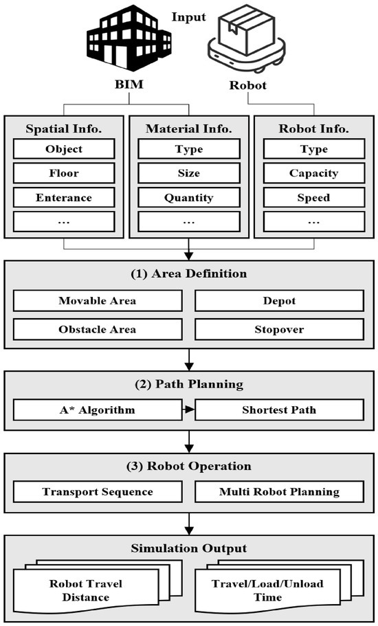
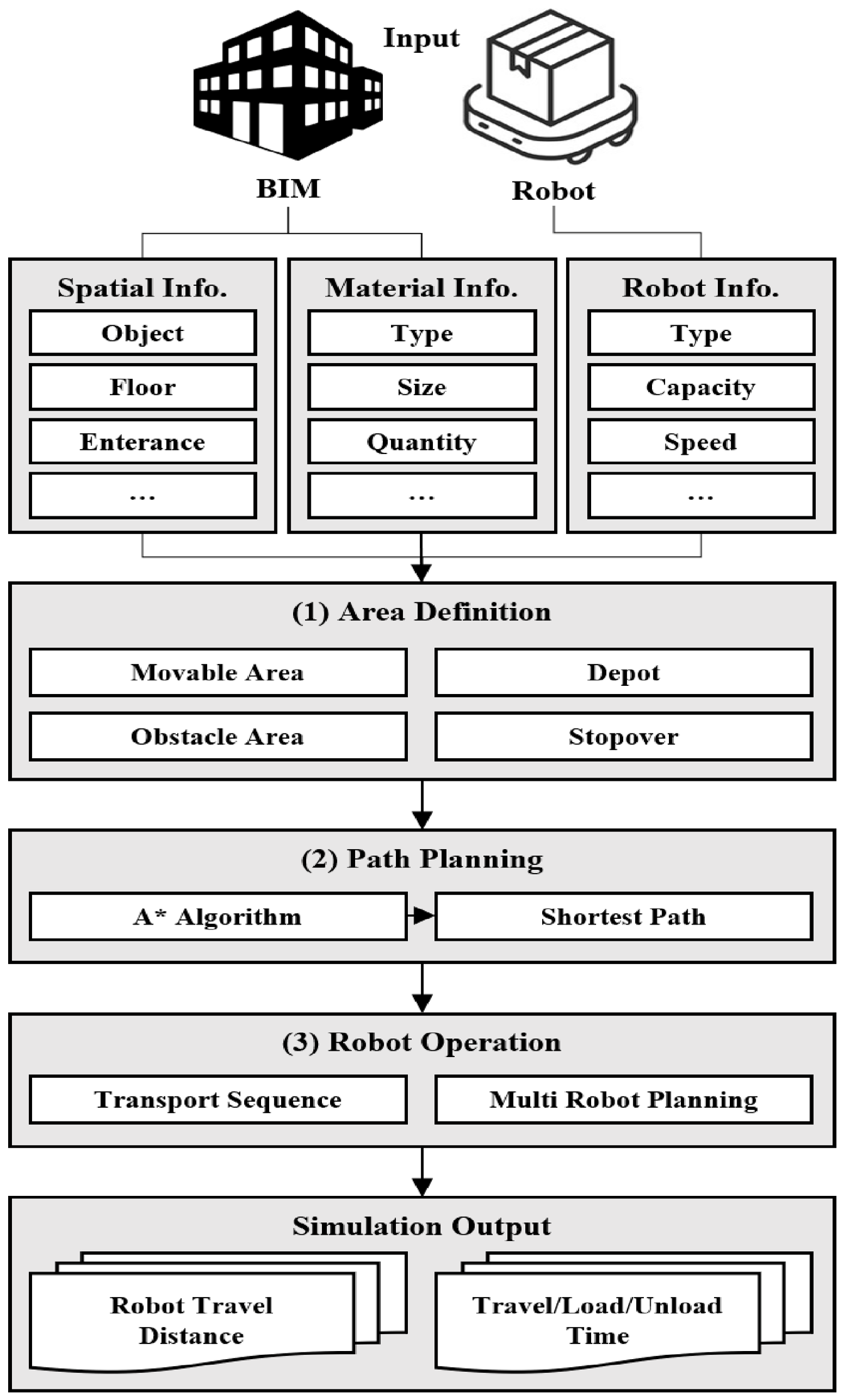
As illustrated in Figure 1, the proposed BIM-enabled simulation proceeds through five consecutive stages: input information, area definition, path planning, robot operation, and simulation output. First, the simulation collects input information from two sources. From the BIM model, it extracts (i) spatial information (e.g., objects, floors, entrances, and other layout elements) and (ii) material information (e.g., material type, size, and quantity) required to define delivery demands. In addition, robot information (e.g., robot type, payload capacity, and travel speed) is provided to reflect operational constraints and performance assumptions.
Figure 1.
Overall Simulation Workflow.
Second, in the area definition stage, BIM-derived geometry is converted into a simulation-ready representation by classifying the workspace into movable areas and obstacle areas, while also defining logistics nodes, including the depot (loading/staging location) and stopovers (material unloading locations/waypoints). This step establishes the feasible navigation space and the set of delivery targets that the robot must serve.
Third, the path planning stage computes collision-free travel costs between the depot and stopovers. In this study, the A* algorithm is used to obtain the shortest path within the movable area while avoiding obstacles, and the resulting path lengths (or travel times derived from robot speed) serve as the basis for evaluating candidate moves during routing decisions.
Fourth, the robot operation stage executes the transport mission by determining (i) the transport sequence (which stopover to visit next) and (ii) the operational policy governing whether the robot continues to another stopover or returns to the depot for reloading under the payload constraint. This module maps the material demand at each stopover to a capacity-constrained delivery process and applies the algorithmic decision logic described in Section 3.4, enabling scenario-based comparison (e.g., rule-based sequential operation versus the proposed efficiency-driven strategy). The framework is also extendable to multi-robot planning by allocating demands and stopovers across multiple robots under shared constraints.
Finally, the simulation generates output indicators that quantify operational efficiency, including robot travel distance and travel/load/unload time, which are used to compare alternative operation strategies and to support pre-deployment what-if analysis for robotized construction logistics.
3.2. BIM-Based Simulation Environment Setup (Area Definition)
The input data provide information for carrying out simulations by reflecting the spatial structure of the construction site, requirements for material transportation, and performance and limitations of the robot. Based on input data, such as the design and process information of the construction site and the robot’s performance information, a virtual simulation environment was implemented in which the robot transported materials. The design information provides details about the structure and spatial configuration of the building being simulated. By utilizing the BIM model, it is possible to build a precise simulation environment that incorporates information about the shape of the building, properties of its components, and the overall structure and location [46]. Process information defines the requirements for material movement according to the progress of the work. This includes data such as type, quantity, and weight, which act as factors in determining the type, load, and possible loading locations of the materials that the robot must transport. The quantity takeoff function in the BIM model can be used to extract the relevant information.
3.3. Robot Information
Robot information refers to the specifications and performance of material transportation robots and is used to develop robot operation considering the weight and volume of the materials. Based on the size information of the robot, a minimum safety distance was set to prevent collisions with walls and obstacles during movement. To optimize the travel paths based on the robot center, a value corresponding to half the width of the robot was used. Additionally, any extra safety distance requested by the user was applied to calculate the minimum safety distance. Through this process, the feasible movement area of the robot was defined.
3.4. Path Planning Using A* Algorithm
This study proposes an efficiency-driven algorithm that combines A* pathfinding with a greedy decision rule to minimize unnecessary trips and maximize transport efficiency. The aim of this algorithm is to have the robot visit multiple destinations in a single trip to minimize unnecessary empty trips and maximize the transport efficiency.
First, to determine the optimal route between unloading points for materials, a heuristic-based A* algorithm was used. The A* algorithm is a pathfinding method that uses an evaluation function combining actual and estimated costs, and is widely used in fields such as robotic path planning and autonomous driving [47]. Because the A* algorithm prioritizes searching for the path with the lowest cost, it can quickly find the shortest route.
The A* algorithm was selected for path planning in this study over alternative approaches such as D* (Dynamic A*) and RRT* (Rapidly exploring Random Tree Star) for the following reasons. D* is designed for dynamic environments where the robot continuously updates path costs in real time as new sensor information is acquired; however, this study assumes a static environment without dynamic obstacles, making the computational overhead of D* unnecessary. RRT* is a sampling-based algorithm well-suited to high-dimensional or unstructured spaces, but requires significantly higher computational cost than A* in structured indoor environments. Braun et al. (2019) [48] demonstrated that in indoor AMR navigation scenarios, RRT* required up to 190 times longer processing time than A* and produced paths approximately 16% longer, confirming that A* offers a more computationally efficient and accurate solution for grid-based indoor environments such as those derived from BIM floor plans.
3.5. Transport Sequence Optimization Using Greedy Search
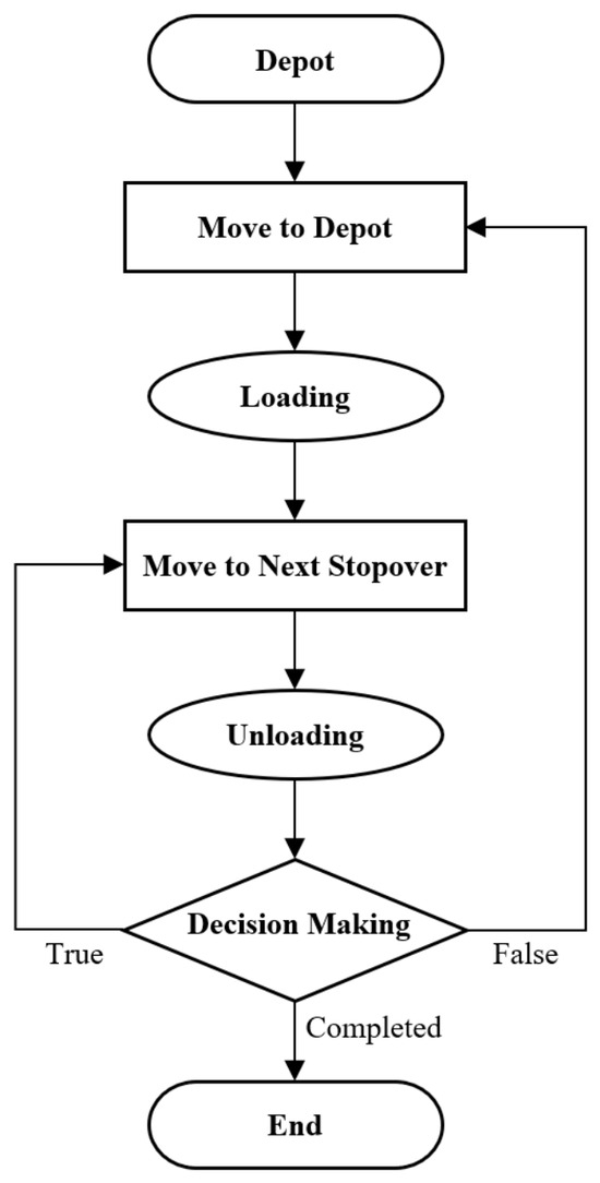
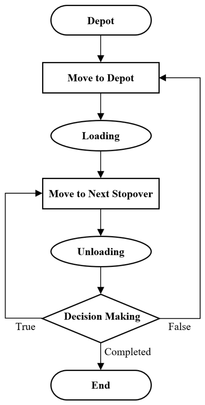
Materials are required at multiple locations, and each location requires different types and amounts of construction materials. This study addresses the Capacitated Vehicle Routing Problem, a classic combinatorial optimization problem that seeks optimal delivery routes for vehicles subject to a maximum load constraint, minimizing total travel distance or time. The proposed algorithm for selecting the next action was designed based on the greedy approach and was used to determine whether the robot, after arriving at the first destination with materials loaded from the starting point, should move directly to the next destination or return to the starting point to reload materials (Figure 2).
Figure 2.
Transport Sequence Decision Making Process.
The robot is guided to continue transporting only if the cost of moving to the next destination (Dnext) is less than or equal to the cost of returning to the starting point (Dreturn). For the first trip, this formula is not applied, and the robot travels along the shortest path; however, for each subsequent stop, this efficiency assessment is repeatedly conducted upon arrival.
A logical error occurs if the permissible distance is calculated using only the robot speed and unloading time for a single material. With this method, the calculated permissible distance for each piece of material becomes excessively large, causing the robot to consistently attempt to move to the next stop in most cases. As a result, the robot may transport only a small amount of material and move inefficiently, or if it reaches its load limit but falls short of the permissible distance, it may not perform additional deliveries, leading to further inefficiency. This suggests that the frequency of material transport trips and the amount of load should be adjusted flexibly according to the scale of the model and the ratio of demand to load capacity.
Therefore, this study introduced a correction factor (k) to address these limitations. This factor serves to flexibly adjust the allowable distance based on the scale of the experiment. For example, if the simulation area is large or if the proportion of materials that a robot can carry at once is small compared to the demand, increasing the value of k expands the allowable distance, encouraging the robot to efficiently cover a wider site. Thus, the value of k is an experimental variable determined by comprehensively considering the scale of the site and transportation efficiency indicators. Through repeated simulations, the optimal value of k that achieves the minimum time and distance is derived.
3.6. Region Partitioning for Multi-Robot Operation
In a Multi-Robot Task Allocation (MRTA) system, preventing the concentration of tasks on specific robots and distributing the workload evenly are key factors that determine the overall system performance [49]. This study proposes a work region partitioning algorithm that distributes the workload evenly among multiple robots and optimizes their movement paths during operation. This study implemented the concept of the geodesic Voronoi diagram and the spatial partitioning technique within a grid environment based on a Revit add-in [50,51].
The region partitioning process starts with defining the geodesic time, which represents the actual travel distance that avoids obstacles on a plane. After specifying the start and waypoints in the grid environment, the geodesic time derived based on the A* algorithm is as follows.
The next step involves selecting the initial representative points (Medoids) that will serve as the operational centers for each robot, based on the number of robots (M) and the number of waypoints (N). The method for selecting the initial representative points begins by designating the demand point with the longest geodesic time from the starting location (Depot) as the first point. Subsequently, the following representative points are sequentially chosen as the demand points with the greatest geodesic time from the already selected points, thereby securing a total of M initial centers for each region. To assign each demand point to a region, an assignment function was used. For workload balance, as previously mentioned, this algorithm employs a weighted assignment method that adds a bias for each region to the distance value.
is a correction term that adjusts the workload of each region i to be relatively larger or smaller. At each iteration, it is updated as follows by comparing the workload of each region with the average workload of all regions .
is a weighting set to prevent region concentration. The workload for each region is calculated by summing the material transport time and the material loading and unloading time.
Finally, the representative point of the assigned region is updated. For the set of stopover assigned to region , the point that minimizes the sum of geodesic travel times to the demand locations within the region is updated as the new representative point
Based on the updated representative points, the process of allocating demand points and adjusting biases is repeated. The final process is concluded when it is determined that the region partitioning has been optimized, which is indicated by the allocation results remaining the same for three consecutive times in the iteration step . Through this iterative optimization process, it is possible to overcome the limitations of simple geographical division and establish a robot operation plan that balances the actual workload and working hours at the site.
4. Case Study
4.1. Simulation Environment and Settings
This chapter describes the application and results of the material transport robot path optimization simulation methodology proposed in this study. The simulation was conducted under two key assumptions regarding the operational environment. First, the experiment was limited to a single floor, excluding vertical transport scenarios such as elevator integration. Second, the environment was assumed to be static, with no dynamic obstacles such as moving workers or equipment during robot operation. This assumption reflects current real-world practice, where material transport robots are typically deployed after working hours—pre-positioning materials for the next day’s work—rather than operating concurrently with workers, as simultaneous operation introduces significant safety risks and efficiency losses. Under these controlled conditions, the experiment isolates the effect of operational planning on robot transport efficiency.
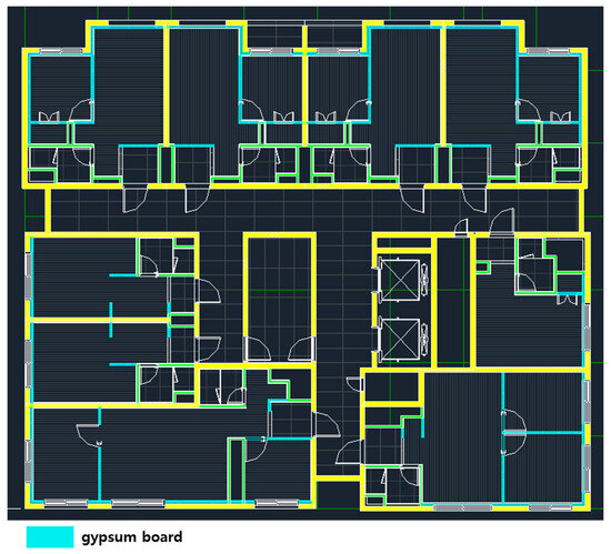
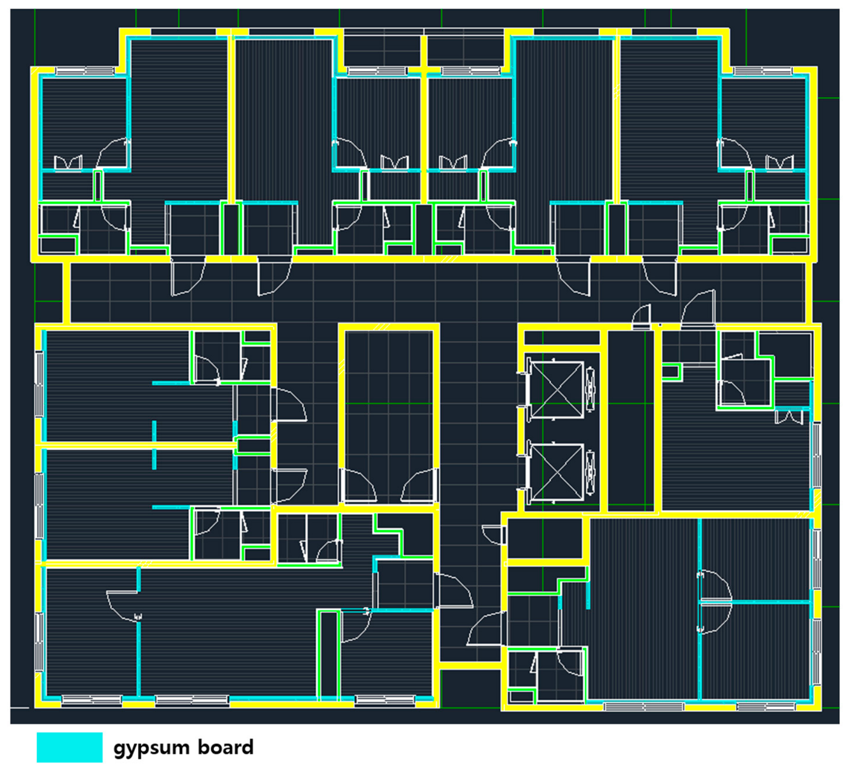
The target project is a studio apartment building in Seoul, South Korea, with a gross floor area (GFA) of 6766.57 square meters. The scope of this study is to optimize the process of transporting and stacking gypsum boards for floor finishing work. The purpose of this simulation was to optimize the path of the material transportation robot as it transported materials from the starting point (main loading area) on site to the material stacking spaces (waypoints) in each room. By minimizing costs, such as the total travel distance and time required for material transport through the simulation, the robot movement path was optimized to maximize the efficiency of robot operation on site. First, based on the design information from the BIM model, the spatial layout and structure of the building were analyzed, and factors affecting the robot’s movement path were identified. Each gypsum board finishing work area within the reference floor was derived, and the material unloading locations were determined. The gypsum board demand for each space was defined by area (m2), and the required amount of gypsum board for each space was determined using Revit (2024)’s material quantity takeoff function (Figure 3 and Table 1). The basic unit of the gypsum board was one sheet, with each sheet weighing 9 kg. Because the maximum load capacity of the robot used is 500 kg, the robot can carry up to 55 sheets (500 kg ÷ 9 kg/sheet = 55 sheets) of gypsum board in one trip.
Figure 3.
Position of the gypsum board in space.
Table 1.
Demand of gypsum boards for each space.
This simulation assumed that a single autonomous mobile robot (AMR) was used to move the gypsum board. The main specifications of the robot are based on the performance of the Peer Robotics RM500 model, as shown in Table 2 [52]. The loading or unloading of materials were set to be assisted by people, and it is assumed that loading or unloading one sheet of gypsum board takes 10 s.
Table 2.
Robot Specifications (Assumptions).
Finally, in this experiment, three alternatives were simulated and comparatively analyzed. Alternative 1 is characterized by sequential operational logic. In this strategy, the robot movement is determined by a predetermined order of stopovers. At the outset of each trip, the robot loaded only the precise amount of material required for the next immediate stopover. Following the unloading of materials at this destination, the robot immediately returns to the original loading location to acquire materials for the subsequent stop. This cycle of “load–go–unload–return” is repeated for every stopover in the sequence.
Alternative 2 represents an intermediate approach that seeks to improve the inefficiencies of Alternative 1. As the first alternative, stopovers are visited in the same predetermined sequence. However, the key difference lies in the loading and return schedule of the robot. At the loading point, the robot loads the materials up to its maximum carrying capacity. It then proceeds to each stopover in the designated sequence and unloads the required materials at each location. The robot only returns to the loading location to replenish its payload once all the materials it is carrying are exhausted. If the remaining materials are insufficient to fulfill the requirements of a subsequent stop, the robot unloads its remaining stock and returns to the loading point to refill its maximum capacity before continuing. This strategy is designed to reduce the number of redundant return trips.
Alternative 3 introduces the proposed methodology for the problem. Unlike the other two alternatives, this strategy does not rely on a predetermined sequence for operational decisions. The robot loads materials to its maximum capacity, mirroring the initial action in Alternative 2. However, the decision to proceed to the next stopover or return to the loading location is not predetermined. Instead, this decision is dynamically determined by the algorithm proposed in this study. This algorithm continuously evaluates the most efficient next step based on real-time conditions, thereby allowing for a flexible and optimized path. This algorithm-driven routing is expected to yield efficiency gains by minimizing travel and maximizing productive time. A summary of the distinct characteristics of each simulation alternative is provided in Table 3.
Table 3.
Comparison of Simulation Alternatives.
4.2. Simulation Result
The primary objective of the simulation was to evaluate and quantify the efficiency of different methodologies in terms of the traveling time and material handling (loading and unloading) time. These results serve as an empirical foundation for a comprehensive comparative analysis of operational strategies. The data presented in Table 4 reveals significant performance discrepancies among the three simulated alternatives.
Table 4.
Simulation Results for Alternatives.
The total distance traveled by the robot is a critical indicator of the efficiency of a strategy, as it directly corresponds to the energy consumption and wear and tear on the equipment. The simulation results show a clear, progressive reduction in the total distance from Alternatives 1 to 3. Alternative 1, with its frequent return trips to the loading location, resulted in the longest travel distance of 447.4 m. Alternative 2, by consolidating trips and returning only when the payload was exhausted, improved significantly, reducing the total distance to 371.1 m. This represents a considerable reduction of approximately 17.1% compared with Alternative 1.
However, the most notable reduction in distance was achieved by Alternative 3. By employing a dynamic algorithm, the robot completed its tasks with a total travel distance of 342.2 m. This marks an approximately 23.5% reduction compared with the baseline Alternative 1. This is a direct result of the algorithm’s ability to optimize the robot path. By deciding whether to proceed to a subsequent stop or return to the base, the system eliminates unnecessary travel legs and ensures that the robot’s path is the most efficient possible, thereby avoiding the non-productive trips that are inherent in the rule-based models of the first two alternatives.
Because the robot speed was assumed to be constant, the result for the robot travel time was proportional to the travel distance. Alternative 3, with its algorithm-driven path optimization, achieved the lowest travel time (3.8 min). Although the reduction in travel time may seem small (less than 2 min), this experiment focused on just one type of material on a single floor. If robots are introduced for the movement of more types of materials across dozens of floors, more work time can be saved.
In terms of handling duration, all alternatives recorded 131.7 min. In this experiment, it was assumed that the time required for loading and unloading was proportional to the quantity of materials. However, if robots are involved in moving a greater variety and quantity of materials, the difference in work time becomes more pronounced. Depending on the type of robot, there are cases where people must directly handle loading and unloading; however, robots that can automatically unload materials have recently been developed. As such, the timing and location of material loading and unloading greatly influence the entire loading/unloading process, and improving this efficiency will also become an important variable in robot operation.
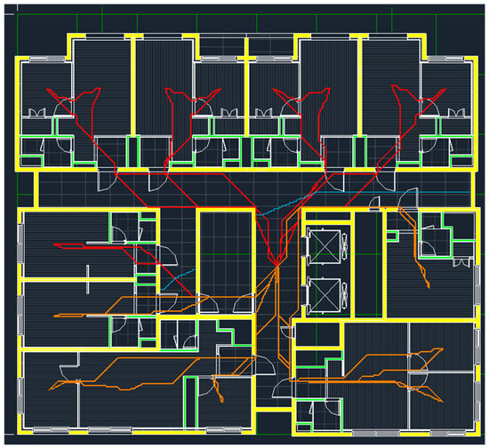
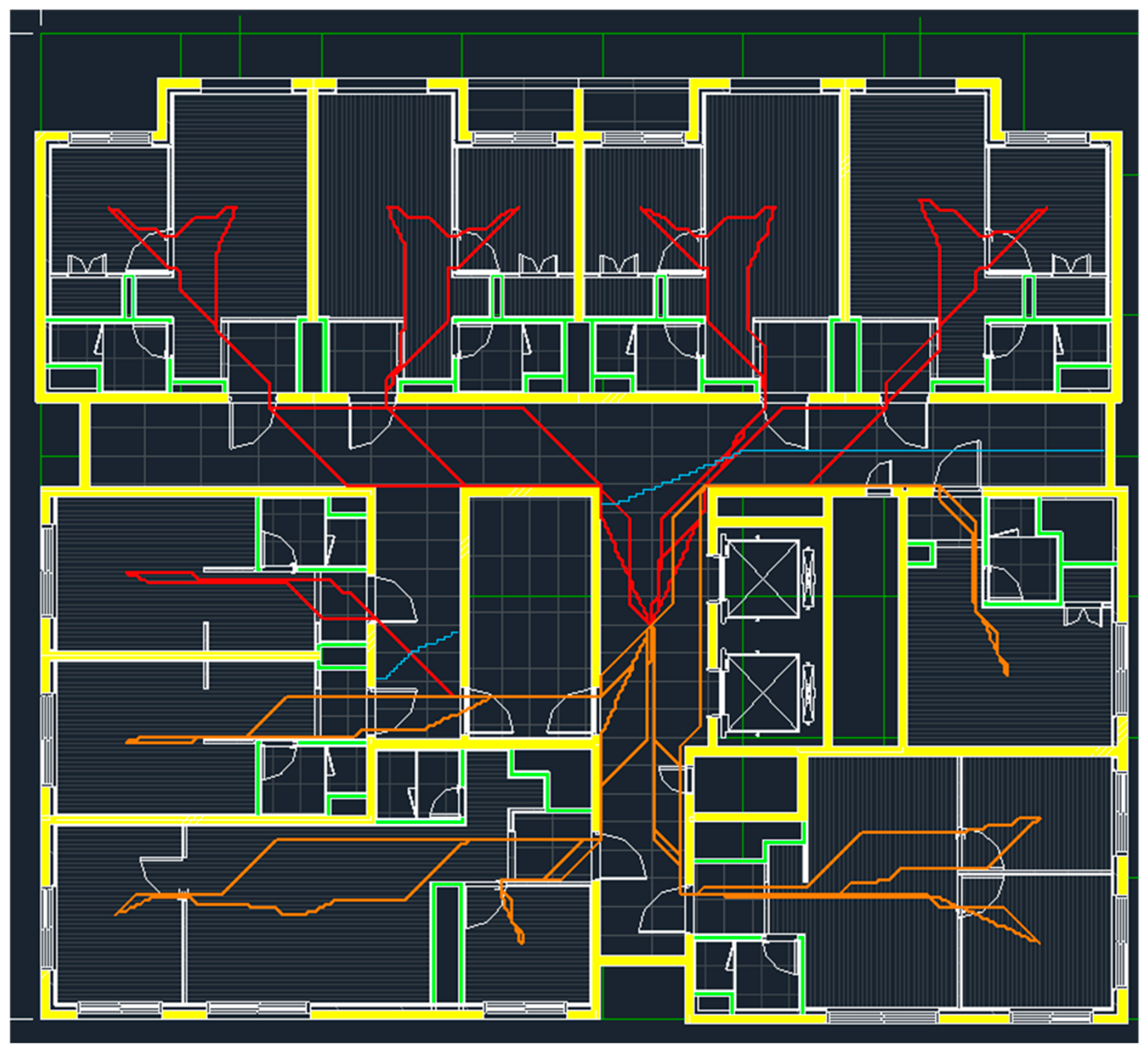
Table 5 presents the simulation results for the multi-robot operation scenario, in which the region partitioning algorithm proposed in Section 3.6 was applied to distribute the workload across two robots (R1 and R2) and compared against the single-robot baseline (R0). R1 and R2 represent the two robots assigned to their respective partitioned regions, where R1 handled the larger share of the workload and R2 the smaller share, as determined by the geodesic Voronoi-based partitioning algorithm. Travel time (T (t), in minutes), material handling time (T (h), in minutes), and travel distance (D, in meters) are reported for each robot and each alternative. The results show that the workload distribution between R1 and R2 is not equal in absolute terms, reflecting the difference in spatial scale and material demand between the two partitioned regions rather than an imbalance in the algorithm. Importantly, the partitioning algorithm does not simply divide the floor plan geographically; it optimizes the assignment of stopovers to minimize total geodesic travel time while balancing the overall workload across robots, as described in Section 3.6. The multi-robot results follow the same trend observed in the single-robot experiment, with Alternative 3 achieving the shortest travel distance and time across both robots, confirming that the efficiency gains of the proposed routing algorithm are maintained under a multi-robot configuration. As illustrated in Figure 4, the floor plan is divided into two operational regions under alternative 3, represented by red and orange path lines respectively, each assigned to an individual robot based on the algorithm proposed in Section 3.6.
Table 5.
Simulation Results for Region Partitioning.
Figure 4.
Example of Multi-Robot Operation Region Partitioning.
5. Discussion
Through this experiment, we compared the simple sequential visiting method with the optimal route method that applies an efficiency evaluation algorithm incorporating a correction factor (k) to the route. The method proposed in this study proved to be far more efficient than the simple sequential method. This result demonstrates that the operational logic of robots significantly affects logistics efficiency at construction sites. Although the experimental results are encouraging, it is crucial from an academic viewpoint to conduct a comprehensive analysis and discuss their limitations. This chapter aims to address these issues by examining both the algorithm and its practical application in the field.
The efficiency judgment algorithm used in this study is one approach to solving the CVRP, and it simulates dynamic decision-making that plans multiple routes (trips) in the optimal order based on the logic that determines whether the robot should move to the next demand point or return to the departure point. The proposed algorithm does not provide an exact solution that calculates all possible paths but rather uses a greedy-based heuristic that determines the next action by evaluating the efficiency at each step. This algorithm is a practical approach for finding ‘local optima.’ In other words, it does not seek a globally optimal solution that minimizes the total travel distance and time required for the entire material transport process by considering all other waypoints that the robot has not yet visited. As this algorithm does not consider the long-term effects of each choice on the overall path, even if it is locally more efficient, it contains a limitation in that it does not guarantee a ‘globally optimal solution’ for the entire transportation process.
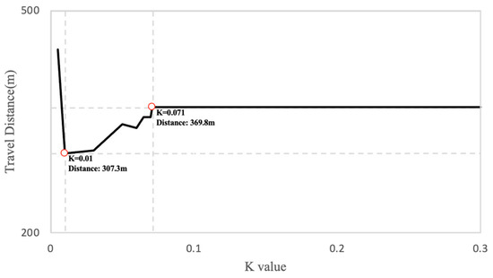
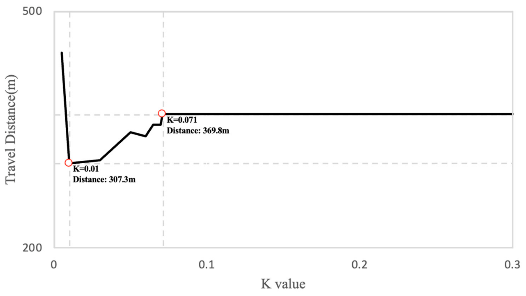
The k value is an experimental variable introduced to adjust the transportation efficiency according to the scale of the site and the ratio of demand to loading capacity. Refining and optimizing the algorithm based on the k value for different site sizes and material demands is an important factor that enhances the versatility of this methodology. Through experiments, k = 0.01 showed optimal results, while the system converges at k = 0.071 (Figure 5). But this value was limited to the given simulation environment with specific project information. In future research, methods for automatically analyzing site size and demand from BIM data to predict the optimal k value may be explored.
Figure 5.
Sensitivity of Total Robot Travel Distance to Correction Factor k.
Deploying robots on-site requires consideration of several additional variables. Simulations conducted in research assume ideal environments; therefore, they have limitations in fully reflecting the complexities of actual construction sites. As mentioned earlier, sites present significant challenges to the autonomous movement of robots owing to constantly changing obstacles (such as temporary structures and dirt piles) and environments (unstable terrain, dust, debris, and severe weather). Such interruptions result in time losses, which are hidden costs that are not reflected in simple distance/time models. It may be worth considering modeling additional costs, such as the time required for rerouting when the robot is blocked by unpredictable obstacles or the time required for manual intervention.
In addition to the travel time and loading/unloading time considered in the simulation, the actual battery status of the robot directly affected the transport efficiency. The energy consumption of the robot varies depending on the weight of the materials being transported and the travel route, which means that the heavier the materials loaded onto the robot, the faster the battery is depleted. Therefore, it is necessary to expand the scope of the problem to an Electric Vehicle Routing Problem (EVRP), which includes battery level, charging time, and energy consumption according to payload as cost functions. This implies that there are more variables to consider in the global optimization problem, and optimization based on machine learning algorithms could be beneficial.
Finally, regardless of the robot’s level of autonomy, on-site robot operations require collaboration with humans. In particular, when it comes to material handling robots, we should not overlook the fact that operator involvement is still necessary for loading and unloading materials, even if the robot moves autonomously. This is a key point that requires a new approach to workforce management. For example, we can consider a scenario in which robots autonomously transport materials at night when workers are not on duty. Although this is an attractive solution for maximizing on-site productivity, it also means that additional personnel will be required to handle loading and unloading tasks at night. Furthermore, even if robots operate during times separated from workers, constant monitoring and emergency response personnel are still needed to address unexpected stops or errors with the robots.
Therefore, at some point, discussions must move beyond the perspective that simply advancing robotics will replace all human labor. It is essential to consider how robots and humans can collaborate efficiently and how workforce management plans should be reestablished with the introduction of robots. Comprehensive simulation and optimization research that considers these technological, human, and on-site factors will determine the practical success of implementing robots in the field.
6. Conclusions
In this study, we addressed the challenges of operating material transport robots at construction sites by proposing a BIM-enabled simulation methodology for their path planning. Our methodology integrates the A* pathfinding algorithm with a greedy decision rule that dynamically determines the next move, yielding a more efficient and robust solution than conventional rule-based approaches. Through a case study involving gypsum board transport on a studio apartment project, the proposed framework achieved more than a 20% improvement in travel efficiency compared with conventional algorithms, validating our initial hypothesis.
Although the current research provides strong evidence for the efficacy of our method, its limitations should be acknowledged. The proposed algorithm is a greedy-based heuristic that finds a ‘local optimum’ at each step rather than a ‘globally optimal solution’ for the entire transport process. More importantly, real-world deployment involves complexity across multiple dimensions: on-site variables such as constantly unpredictable obstacles and environmental conditions like dust and severe weather; robot variables such as sensor limitations and the need for frequent dynamic path replanning, which consumes significant battery life; and human variables such as the need for personnel for robot management and emergency response. Optimizing this array of variables remains a challenging problem, and future research should pursue machine learning-based optimization capable of learning from and adapting to these complexities. Although such “black box” solutions may not be provably optimal, they can still provide a blueprint for a more robot-friendly construction site. Practical application strategies that account for on-site characteristics and the technological maturity of robots are also needed to ensure a smooth transition from simulation to real-world deployment.
In addition, simulation fidelity is directly determined by the level of detail in the BIM model. While the current framework relies on spatial geometry and material quantity, richer BIM data could support more realistic simulations—for example, physical properties (material type, slope) for more accurate battery consumption modeling, or robot-elevator communication protocols for multi-floor planning. Integration with 4D BIM, which links geometry to the construction schedule, would further allow the framework to account for time-varying site conditions such as temporary structures, formwork, and material stockpiles that appear and disappear as construction progresses. Ultimately, as BIM models grow more comprehensive, the proposed framework can evolve toward a full digital twin-based robot simulation environment that more faithfully reflects real construction site conditions.
Despite these limitations, the primary strength of this study lies in its empirical demonstration that the proposed framework can improve on-site robot operational efficiency. Another key strength is its ability to incorporate robot operation planning from the design phase by leveraging BIM-based construction site information, enabling seamless integration between building design and robotic logistics planning. This study therefore provides a foundational and practical step toward a robot-efficient construction environment in which humans and robots can work together more effectively.
Author Contributions
Conceptualization, J.Y.C. and J.G.L.; methodology, J.Y.C. and T.H.H.; validation, T.H.H., J.Y.C. and J.G.L.; data curation, T.H.H.; writing—original draft preparation, T.H.H., J.Y.C. and J.G.L.; writing—review and editing, J.G.L.; supervision, J.G.L.; project administration, J.G.L. All authors have read and agreed to the published version of the manuscript.
Funding
This work is supported by the Korea Agency for Infrastructure Technology Advancement (KAIA) grant funded by the Ministry of Land, Infrastructure and Transport (Grant No. RS-2026-25528110) and the Education and Research promotion program of KOREATECH in 2024.
Data Availability Statement
Data that support the findings of this study are available from the corresponding author upon reasonable request.
Conflicts of Interest
The authors declare no conflicts of interest.
Abbreviations
The following abbreviations are used in this manuscript:
| BIM | Building Information Modeling |
| SLAM | Simultaneous Localization and Mapping |
| VRP | Vehicle Routing Problem |
| CVRP | Capacitated Vehicle Routing Problem |
| AGV | Automated Guided Vehicle |
| AMR | Autonomous Mobile Robot |
References
- Lloyd’s Register Foundation. Engineering Safer Workplaces: Global Trends in Occupational Safety and Health. World Risk Poll Report. 2024. Available online: https://www.lrfoundation.org.uk/publications/engineering-safer-workplaces-global-trends-in-occupational-safety-and-health (accessed on 26 August 2025).
- International Labour Organization. Construction: A Hazardous Work. 2015. Available online: https://www.ilo.org/resource/construction-hazardous-work (accessed on 26 August 2025).
- Barbosa, F.; Woetzel, J.; Mischke, J. Reinventing Construction: A Route of Higher Productivity; McKinsey Global Institute: San Francisco, CA, USA, 2017. [Google Scholar]
- Kim, J.; Yoon, I.; Jung, M.; Joo, S.; Park, S.; Hong, Y.; Cho, J.; Park, M. Establishment of Measurement Standards for Productivity Assessment in Construction Project. Korean J. Constr. Eng. Manag. 2022, 23, 3–12. [Google Scholar]
- Yu, J.; Son, B. A Study on Benchmarking the Countermeasures Strategy for Tackling the Construction Labor Shortage—Focusing UK’s MMC & Singapore’s Buildability. Korean J. Constr. Eng. Manag. 2022, 23, 54–64. [Google Scholar] [CrossRef] [Scilit]
- Alumbugu, P.; Shakantu, W.; Tsado, A.; Ola-awo, W. Efficient utilisation of automation in construction materials-handling processes. Acta Structilia 2022, 29, 33–57. [Google Scholar] [CrossRef] [Scilit]
- Wijesinghe, S.M.N.B.; Wijerathna, M.R.D.P.; Ranadewa, K.A.T.O.; Parameswaran, A. Exoskeleton for health and safety in construction workers: A literature review. In Proceedings of FARU Conference 2024; University of Moratuwa: Moratuwa, Sri Lanka, 2024. [Google Scholar] [CrossRef] [Scilit]
- Choi, S.D.; Trout, D.; Earnest, S.; Garza, E. Exoskeletons: Potential for Preventing Work-Related Musculoskeletal Injuries and Disorders in Construction Workplaces. NIOSH Science Blog, 3 February 2022. Available online: https://www.cdc.gov/niosh/bulletin/2022/exoskeletons-construction.html (accessed on 26 August 2025).
- Lee, S.; Moon, J.I. Case studies on glazing robot technology on construction sites. In 2015 Proceedings of the 32nd ISARC, Oulu, Finland, 15–18 June 2015; IAARC: Cambridge, UK, 2015; p. 1. [Google Scholar]
- Spinelli, F.A.; Zhai, Y.; Nan, F.; Egli, P.; Nubert, J.; Bleumer, T.; Miller, L.; Hofmann, F.; Hutter, M. Large Scale Robotic Material Handling: Learning, Planning, and Control. arXiv 2025, arXiv:2508.09003. [Google Scholar]
- KEBA. Mobile Robots in the Logistics Industry. 2025. Available online: https://www.keba.com/en/news/industrial-automation/mobile-robots-in-the-logistics-industry (accessed on 26 August 2025).
- IDTechEx. Mobile Robotics in Logistics, Warehousing and Delivery 2022–2042. Available online: https://www.idtechex.com/en/research-report/mobile-robotics-in-logistics-warehousing-and-delivery-2022-2042/855 (accessed on 26 August 2025).
- ResearchGate. Motion Planning of Mobile Robots for Autonomous Navigation on Uneven Ground Surfaces—Scientific Figure. Available online: https://www.researchgate.net/figure/Mobile-robot-navigation-on-uneven-surfaces-at-a-typical-construction-site_fig1_348754558 (accessed on 9 July 2026).
- Uchiito, H.; Bhat, A.; Kusaka, K.; Zhang, X.; Kinjo, H.; Uehara, H.; Koyama, M.; Natsume, S. Robotics Under Construction: Challenges on Job Sites. arXiv 2025, arXiv:2506.19597. [Google Scholar]
- Azobuild. Construction Robotics in Extreme Environments: From Earth to Space. 2025. Available online: https://www.azobuild.com/news.aspx?newsID=23737 (accessed on 26 August 2025).
- Phillips, T.G.; Guenther, N.; McAree, P.R. When the dust settles: The four behaviors of lidar in the presence of fine airborne particulates. J. Field Robot. 2017, 34, 985–1009. [Google Scholar] [CrossRef] [Scilit]
- Botshare. CASE STUDY: SIMPLE LOGISTICS PROCESSES AUTOMATION WITH LiDAR SLAM AMR. 2023. Available online: https://www.botshare.blog/case-study-simple-logistics-processes-automation-with-lidar-slam-amr/ (accessed on 26 August 2025).
- Dusty Robotics. What are the Barriers to Adopting Robotics in Construction. 2023. Available online: https://www.dustyrobotics.com/articles/what-are-the-barriers-to-adopting-robotics-in-construction (accessed on 26 August 2025).
- Bullo, F.; Frazzoli, E.; Pavone, M.; Savla, K.; Smith, S.L. Dynamic vehicle routing for robotic systems. Proc. IEEE 2011, 99, 1482–1504. [Google Scholar] [CrossRef] [Scilit]
- Ralphs, T.K.; Kopman, L.; Pulleyblank, W.R.; Trotter, L.E. On the capacitated vehicle routing problem. Math. Program. 2003, 94, 343–359. [Google Scholar] [CrossRef] [Scilit]
- Yoon, H.; Lee, J.; Hwang, J.; Kang, H.; Park, S.; Kang, L. Method of Deriving Activity Relationship and Location Information from BIM Model for Construction Schedule Management. Korean J. Constr. Eng. Manag. 2022, 23, 33–44. [Google Scholar]
- Kim, H.; Nam, J. Applying BIM Standard Guideline to Expressway BIM Results and Drawing its Improvement Measure for Project Management. Korean J. Constr. Eng. Manag. 2025, 82–88. [Google Scholar]
- Zhang, L.; Zhao, J.; Long, P.; Wang, L.; Qian, L.; Lu, F.; Song, X.; Manocha, D. An autonomous excavator system for material loading tasks. Sci. Robot. 2021, 6, eabc3164. [Google Scholar] [CrossRef] [Scilit] [PubMed]
- Standard Bots. The Power of Robotics in Construction. 23 April 2025. Available online: https://standardbots.com/blog/revolutionizing-construction-the-power-of-robotics (accessed on 26 August 2025).
- Davich, T. Material Handling Solutions: A Look into Automated Robotics; Resource Document; University of Wisconsin-Madison: Madison, WI, USA, 2010. [Google Scholar]
- Pizoń, J.; Wójcik, Ł.; Gola, A.; Kański, Ł.; Nielsen, I.E. Autonomous mobile robots in automotive remanufacturing: A case study for intra-logistics support. Adv. Sci. Technol. Res. J. 2024, 18, 213–230. [Google Scholar] [CrossRef] [Scilit] [PubMed]
- Mission Design & Automation. How AMRs Maximize Material Transfer Efficiency and Safety in Manufacturing. Available online: https://missiondesignauto.com/learning-centers/how-amrs-maximize-material-transfer-efficiency/ (accessed on 26 August 2025).
- Standard Bots. AMR Logistics: The Basics. 3 July 2025. Available online: https://standardbots.com/blog/amr-logistics (accessed on 26 August 2025).
- Vecna Robotics. Comparing AMRs and AGVs: What’s Your Best Option. Available online: https://www.vecnarobotics.com/amr-vs-agv/ (accessed on 26 August 2025).
- Teradyne. Autonomous Mobile Robots. Available online: https://www.teradyne.com/robotics/autonomous-mobile-robots/ (accessed on 26 August 2025).
- Genesis Systems. Robotic Material Handling and Tending: A Basic Overview. Available online: https://www.genesis-systems.com/blog/robotic-material-handling-and-tending-a-basic-overview (accessed on 26 August 2025).
- Kawasaki Robotics. Material Handling. Available online: https://kawasakirobotics.com/asia-oceania/applications/material-handling/ (accessed on 26 August 2025).
- Coherent Market Insights. Material Handling Robotics Market Size and Trends, 2025–2032 [Market Research Report]. Available online: https://www.coherentmarketinsights.com/industry-reports/material-handling-robotics-market (accessed on 26 August 2025).
- Boston Dynamics. Spot—The Agile Mobile Robot. Available online: https://bostondynamics.com/products/spot/ (accessed on 26 August 2025).
- Oceaneering. Oceaneering Mobile Robotics (OMR). Available online: https://www.oceaneering.com/oceaneering-mobile-robotics-omr/ (accessed on 26 August 2025).
- Ryde, J.; Hillier, N. Performance of laser and radar ranging devices in adverse environmental conditions. J. Field Robot. 2009, 26, 712–727. [Google Scholar] [CrossRef] [Scilit]
- Agility Robotics. Digit—Spec Sheet. Available online: https://www.agilityrobotics.com/resources/spec-sheet (accessed on 22 September 2025).
- Figure AI. F.03 Battery Development. 17 July 2025. Available online: https://www.figure.ai/news/f-03-battery-development (accessed on 22 September 2025).
- SYSTEMA. Automated Material Handling Systems. Available online: https://www.systema.com/digital-transformation/automated-material-handling-systems (accessed on 26 August 2025).
- Vitrans Conveyor. 8 Types of Material Handling Equipment Used in Construction. 24 February 2025. Available online: https://www.vitrans-conveyor.com/2025/02/24/8-types-of-material-handling-equipment-used-in-construction/ (accessed on 26 August 2025).
- Mobile Industrial Robots. MiR250—Specifications. Available online: https://mobile-industrial-robots.com/products/robots/mir250/specifications (accessed on 20 September 2025).
- Frías, E.; Díaz-Vilariño, L.; Balado, J.; Lorenzo, H. From BIM to Scan Planning and Optimization for Construction Control. Remote Sens. 2019, 11, 1963. [Google Scholar] [CrossRef] [Scilit]
- Park, S.; Yoon, S.; Ju, S.; Heo, J. BIM-based scan planning for scanning with a quadruped walking robot. Autom. Constr. 2023, 152, 104911. [Google Scholar] [CrossRef] [Scilit]
- Harrou, F.; Zeroual, A.; Hittawe, M.M.; Sun, Y. Chapter 2—Road traffic modeling. In Road Traffic Modeling and Management: Using Statistical Monitoring and Deep Learning; Elsevier: Amsterdam, The Netherlands, 2021; pp. 15–63. [Google Scholar]
- Harrou, F.; Zeroual, A.; Hittawe, M.M.; Sun, Y. Chapter 5—Traffic congestion detection: Data-based techniques. In Road Traffic Modeling and Management: Using Statistical Monitoring and Deep Learning; Elsevier: Amsterdam, The Netherlands, 2021; pp. 141–195. [Google Scholar]
- Ha, D.; Yu, Y.; Choi, J.; Kim, S.; Koo, B. Integrating a Machine learning-based space classification model with an automated interior finishing system in BIM models. Korean J. Constr. Eng. Manag. 2023, 24, 60–73. [Google Scholar]
- Chu, L.; Wang, Y.; Li, S.; Guo, Z.; Du, W.; Li, J.; Jiang, Z. Intelligent vehicle path planning based on optimized a* algorithm. Sensors 2024, 24, 3149. [Google Scholar] [CrossRef] [Scilit] [PubMed]
- Braun, J.; Brito, T.; Lima, J.; Costa, P.; Costa, P.; Nakano, A. A Comparison of A* and RRT* Algorithms with Dynamic and Real Time Constraint Scenarios for Mobile Robots. In Proceedings of the 9th International Conference on Simulation and Modeling Methodologies, Technologies and Applications (SIMULTECH 2019); SciTePress: Setubal, Portugal, 2019; pp. 398–405. [Google Scholar]
- Lee, D.-H.; Zaheer, S.A.; Han, J.-H.; Kim, J.-H.; Matson, E. Competency adjustment and workload balancing framework in multirobot task allocation. Int. J. Adv. Robot. Syst. 2018, 15, 1729881418812960. [Google Scholar] [CrossRef] [Scilit]
- Aronov, B. On the geodesic Voronoi diagram of point sites in a simple polygon. In Proceedings of the Third Annual Symposium on Computational Geometry; Association for Computing Machinery: New York, NY, USA, 1987; pp. 39–49. [Google Scholar]
- Wu, L.; García García, M.Á.; Puig Valls, D.; Solé Ribalta, A. Voronoi-based space partitioning for coordinated multi-robot exploration. J. Phys. Agents 2007, 1, 37–44. [Google Scholar] [CrossRef] [Scilit]
- Peer Robotics. RM500—Product Page. Available online: https://www.peerrobotics.ai/products/rm-series/rm500 (accessed on 22 September 2025).

Disclaimer/Publisher’s Note: The statements, opinions and data contained in all publications are solely those of the individual author(s) and contributor(s) and not of MDPI and/or the editor(s). MDPI and/or the editor(s) disclaim responsibility for any injury to people or property resulting from any ideas, methods, instructions or products referred to in the content. |
© 2026 by the authors. Licensee MDPI, Basel, Switzerland. This article is an open access article distributed under the terms and conditions of the Creative Commons Attribution (CC BY) license.