A Quantile Decision-Support Model for Predicting Court Judgment Amounts in Multi-Family Housing Defect Litigation

Abstract

This study aims to develop a pre-litigation decision-support model that estimates the expected court judgment amount in multi-family housing defect litigation using only information available before a suit is filed. To this end, 106 final-instance South Korean court judgments (2014–2025) were compiled and decomposed into 33,997 item-level records, on which a three-layer hybrid model was built. The first layer is an ordinary least squares (OLS) regression of the area-normalized award on three pre-filing variables—elapsed months, log exclusive area, and log claimed amount (R² = 0.626). The second layer is a multinomial logistic classifier predicting the liability limitation band, with a ±1-band accuracy of 94.4%. The third layer is a probabilistic quantile layer that combines the two to output five quantiles. Under leakage-free five-fold cross-validation, the model achieved a Q50 mean absolute percentage error (MAPE) of 28.4% with well-calibrated interval coverage (50% interval—49.1%; 80% interval—79.2%). A preliminary external validation on 22 independent cases gave a MAPE of 21.4% (bootstrap 95% CI [15.0%, 28.6%]). The interquartile band (Q25–Q75) provides both parties an objective non-litigation settlement range, offering a shared basis to move from adversarial litigation toward earlier, information-based settlement.

1. Introduction

Over the past half-century, South Korea’s housing has shifted fundamentally from single-family residences to multi-family housing. According to the 2024 Population and Housing Census of Statistics Korea (now the Ministry of Data and Statistics) [1], multi-family housing accounts for 15.82 million of the country’s 19.87 million dwellings (79.6%). Real assets—mainly real estate—make up about 75.8% of the average household’s gross assets [2]. This pattern recurs across East Asia. In Japan, multi-family housing reached a record 44.9% of occupied dwellings (24.97 million units) in the 2023 Housing and Land Survey [3], and housing and residential land form 71.0% of household net worth [4]. In China, where 63.9% of the population was urban as of the 2020 census [5], post-1998 housing reform shifted urban supply overwhelmingly to apartment complexes, and housing alone constitutes 59.1% of urban households’ total assets [6]. Although each country defines household assets differently, all three show that multi-family housing is both the main form of residence and the largest component of household wealth. Against this backdrop, defects in multi-family housing carry broad social and economic significance.

Disputes over defects in multi-family residential buildings are a persistent and costly problem worldwide, not only in any single jurisdiction. At their core lies an information asymmetry between contractors and residents over the true scope and cost of defects. This is structurally analogous to the “market for lemons” first described by Akerlof [7], in which asymmetric information about quality drives adverse selection. Crommelin et al. [8] demonstrated this dynamic empirically in Australian residential defect disputes, where neither party can reliably assess the other’s information before a claim crystallizes. Similar defect burdens have been documented across jurisdictions—in multi-unit Australian dwellings [9], in strata common property [10], and in low-rise residential buildings [11]. When such disputes escalate to litigation, both parties incur the transaction costs of adversarial proceedings [12]—appraisal, legal fees, and years of delay—often pursuing monetary compensation in place of substantive repair. Because litigation is costly relative to settlement, an economic analysis of dispute resolution predicts that parties settle when each can foresee its likely outcome [13]; the obstacle is precisely the absence of such a foreseeable estimate before filing.

In South Korea, where this study is set, the scale of the problem is substantial. Over the past five years (2021–2025), between about 320,000 and 410,000 multi-family housing units have been completed each year [14]. This continually expands the housing stock at risk of defects. The Ministry of Land’s defect-review and dispute-mediation committee handled roughly 4600 defect disputes annually between 2021 and 2025 (4732 cases in 2021 and 4761 in 2025), of which 68.3% (7448 of 10,911 screened items) were adjudged genuine defects [15]. Civil defect lawsuits are not isolated in official statistics, but this caseload illustrates the prevalence of such disputes. Among the 106 cases examined in this study, suits were filed on average 3.9 years after the completion inspection, with 69.8% concentrated between the third and fifth year. This is just before the statutory warranty expires, when the residents’ representative body files to interrupt the limitation period. Korean multi-family housing defect litigation operates on a distinctive institutional base: claim assignment from individual owners to a residents’ representative body, a court-applied liability limitation ratio, and statutory exclusion periods (analogous to a statute of repose). The underlying economic problem, however, is a global one; at the moment the decision to sue is made, neither party has an objective estimate of the likely judgment amount. The consequence is a structural pattern of over-claiming, litigation that in our sample averages 31.6 months, and accumulated information asymmetry that entrenches adversarial compensation over repair. This gap is not for lack of prior research; rather, the existing literature shares common limitations that are reviewed in Section 2, and that this study addresses.

This study addresses these gaps by developing a model that estimates the expected judgment amount in multi-family housing defect litigation using only variables available before a suit is filed. It validates this model both internally and on an independent external sample. The model has a three-layer hybrid architecture. The first layer is an ordinary least squares (OLS) regression of the area-normalized award on three pre-filing variables (elapsed months, log exclusive area, log claimed amount). The second is a multinomial logistic classifier that predicts the liability limitation band, and the third is a probabilistic quantile layer that combines the two to output five quantiles (Q10–Q90) rather than a single point estimate. The design deliberately separates the liability limitation ratio from the regression target and applies it exactly once at the conversion stage, correcting an algebraic double-application that would otherwise systematically under-predict the award. Methodologically, the model draws on established statistical foundations—heteroskedasticity-robust estimation [16] (with the consistent covariance estimator of [17]), multinomial choice modeling [18], and standard logistic regression procedure [19]. It further draws on quantile-based interval estimation (Koenker and Bassett [20]; Koenker and Hallock [21]; see also [22,23]), conformalized quantile regression for interval reliability [24,25], cross-validation [26], and the bootstrap [27,28]. The model adopts a predictive rather than explanatory modeling stance (Shmueli [29]; Breiman [30]). Recent reviews of predictive uncertainty estimation [31] and explainable AI cost prediction with confidence intervals [32] further support interval-valued over point estimation. The inflation adjustment by construction cost index follows time-series treatments of such indices [33].

The study makes three contributions. First, it provides a pre-litigation estimation model usable at the decision-to-sue stage. It is built on the largest multi-family-housing defect judgment dataset assembled for this purpose in South Korea (106 cases; 33,997 item-level records spanning 2014–2025). Second, beyond the internal cross-validation commonly used in prior work, it adds a preliminary external validation on independent cases (n = 22), providing out-of-sample evidence that prior studies in this area generally did not report. Third, the single estimate serves both parties’ distinct decisions. The model presents the lower quartile (Q25) as a conservative recovery floor for residents and the upper quartile (Q75) as a conservative loss ceiling for contractors, giving an objective basis for a non-litigation settlement range. This study addresses two research questions, as follows: (RQ1) Can a model using only pre-filing information achieve calibrated interval estimates of the judgment amount? (RQ2) Does restricting inputs to pre-filing variables generalize to independent, unseen cases?

The empirical calibration in this study is necessarily grounded in Korean judgments. In principle, however, the model’s three-layer architecture is adaptable to other jurisdictions with re-estimation on local data. This includes settings where residential building defects give rise to collective or representative disputes, such as the Australian strata and multi-owned housing contexts documented in [9,10,11]. The remainder of the paper reviews related literature (Section 2), describes the data and research methodology (Section 3), reports the analysis results (Section 4), discusses the implications and limitations of the model (Section 5), and presents the conclusions (Section 6).

2. Literature Review

The literature relevant to this study spans three streams: the economics of information asymmetry and dispute resolution, empirical studies of housing defects and their litigation, and quantitative or machine-learning approaches to predicting construction dispute outcomes. This section reviews these streams without distinguishing domestic from international work, and identifies the gaps that motivate the model developed here.

2.1. Information Asymmetry and the Economics of Dispute Resolution

The conceptual foundation of this study is the economics of asymmetric information. Akerlof [7] showed that when buyers cannot verify quality before purchasing, adverse selection can degrade an entire market—a mechanism directly analogous to housing defect disputes, in which residents cannot observe the true scope or cost of latent defects before a claim is filed. Crommelin et al. [8] confirmed this dynamic empirically in Australian multi-owned housing, where neither party can reliably assess the other’s information beforehand. From a transaction cost perspective, Williamson [12] frames adversarial litigation as a costly governance mechanism, while Shavell [13] shows analytically that parties settle when each can foresee the likely outcome. These works establish why an objective, pre-filing estimate of the expected judgment is valuable, but they remain theoretical and do not provide an operational estimation tool. Recent empirical work applying machine learning directly to judicial outcome prediction—for example, Medvedeva et al.’s [34] models of European Court of Human Rights decisions—supports a premise foundational to the present study. This premise holds that legal outcomes contain statistically learnable regularities that can be estimated in advance of a case’s resolution. Section 2.3 reviews this and related predictive literature in detail. Beyond the model’s technical validity, however, its practical adoption also depends on the wider information environment in which the parties operate. Parties’ trust in formal dispute resolution institutions can itself be shaped by external information flows, including social media-driven misinformation [35]—a dependency relevant whenever a decision-support tool, including the one proposed here, is introduced into practice.

2.2. Empirical Studies of Housing Defects and Defect Litigation

A substantial body of empirical work documents the prevalence and cost of housing defects. Studies of multi-unit Australian dwellings [9], strata common property [10], and low-rise residential buildings [11] characterize defect types, causes, and risks, but do not extend to estimating litigation outcomes. In the Korean context, a series of studies has examined defect-repair costs relative to construction costs and post-handover quality management [36,37], and Ko et al. [38] fit a regression model to predict judgment amounts. However, these studies rely on variables fixed only during litigation—recognized-defect amounts, the assignment ratio, or court-appraised costs—which are unavailable at the pre-filing stage, and none of these report an independent external validation. Park and Seo [39] likewise present a linear regression on a 100-case sample without out-of-sample testing. The common limitation is twofold—dependence on post-hoc variables and the absence of a validation framework.

2.3. Predictive and Machine-Learning Approaches to Construction Disputes

Internationally, machine learning- and case-based approaches to construction disputes have proliferated. An early hybrid artificial neural network (ANN)–case-based reasoning (CBR) model addressed disputed change orders [40]; Arditi and Pulket [41] predicted litigation outcomes with an integrated artificial intelligence model, and Chou [42], Mahfouz and Kandil [43], Un et al. [44], and Sarı et al. [45] classified dispute outcomes. Related work has applied natural language processing to residential defect dispute support [46], machine learning to defect-repair task classification [47], and decision support systems to early dispute prediction [48]. These studies demonstrate the feasibility of data-driven dispute analysis, but they target categorical outcomes (win/lose or resolution mode) rather than the continuous, probabilistic estimation of the judgment amount itself, and most depend on information available only after a suit is filed.

Complementary work on the Turkish construction sector has examined dispute sources and litigation dynamics through court-file analysis, finding debit and credit and defective product issues to be the most frequent dispute categories and reassessment decisions to dominate appellate outcomes [49,50]. A related study identifies precautions—such as contract clarity, auditing effectiveness, and alternative dispute resolution—that practitioners can adopt to reduce the incidence of disputes escalating to litigation [51].

Read collectively, these systems [40,41,44,46,48] constitute the closest prior decision support analogues to the present study. The present model is distinguished from all five by (i) restricting inputs to pre-filing information, (ii) outputting a calibrated probabilistic interval rather than a categorical or point prediction, and (iii) independent external validation.

The machine learning-based prediction of judicial outcomes has also been studied outside the construction domain, most notably in European Court of Human Rights case outcome prediction [34,52]. The methodological cautions raised in that study—distinguishing genuine legal signal from surface textual patterns—parallel the present study’s restriction of inputs to verifiable pre-filing variables. More broadly, the deployment of predictive tools in public administration contexts raises shared concerns of transparency and algorithmic accountability [53]. These concerns extend naturally to judicial decision support tools such as the one proposed here. The present model’s restriction of inputs to verifiable pre-filing information, and its interval-valued rather than point output, are concrete design choices that respond to these concerns.

2.4. Research Gaps

Across these streams, three gaps are recurrently observed. First, reliance on post-hoc variables; most estimation studies use inputs fixed only during litigation and therefore cannot be applied at the pre-filing stage when an estimate is actually needed. Second, the limited use of large, linked datasets; structured cost data and unstructured legal issue data are rarely linked through a common case identifier so that statistical estimation and doctrinal explanation can be produced for the same cases. Third, limited validation; error metrics on separated training and validation samples are seldom reported, and an independent external validation is rarely performed—an omission that, for a predictive model, makes reported accuracy difficult to distinguish from overfitting. The present study addresses these gaps by developing a pre-filing estimation model and validating it both internally and on an independent external sample.

3. Data and Research Methodology

3.1. Research Design and Data Architecture

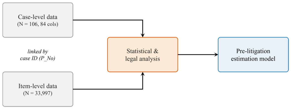
This study develops a model that estimates the expected court-awarded judgment amount in multi-family housing defect lawsuits using only information available before a suit is filed. The analytical basis is a two-layer dataset linked by a common case identifier (P_No, P001–P106). The first layer is a case-level metadata table of 84 columns extracted from 106 final instance judgments, covering the macro-structure of each dispute (claimed, appraised, and awarded amounts; liability limitation ratio; litigation duration). The second layer decomposes the defect schedule of the same 106 judgments into 33,997 item-level records classified by work type, location, time of occurrence, and amount, capturing the micro-structure of defects. Linking the two layers by P_No allows the statistical and legal patterns of the same case to be analyzed jointly (Figure 1). The present paper focuses on the case-level layer (N = 106) and the external validation sample (N = 22); within this paper the item-level records are used only to characterize the dispute structure (Section 4.1), while the full item-level analysis is reported separately.

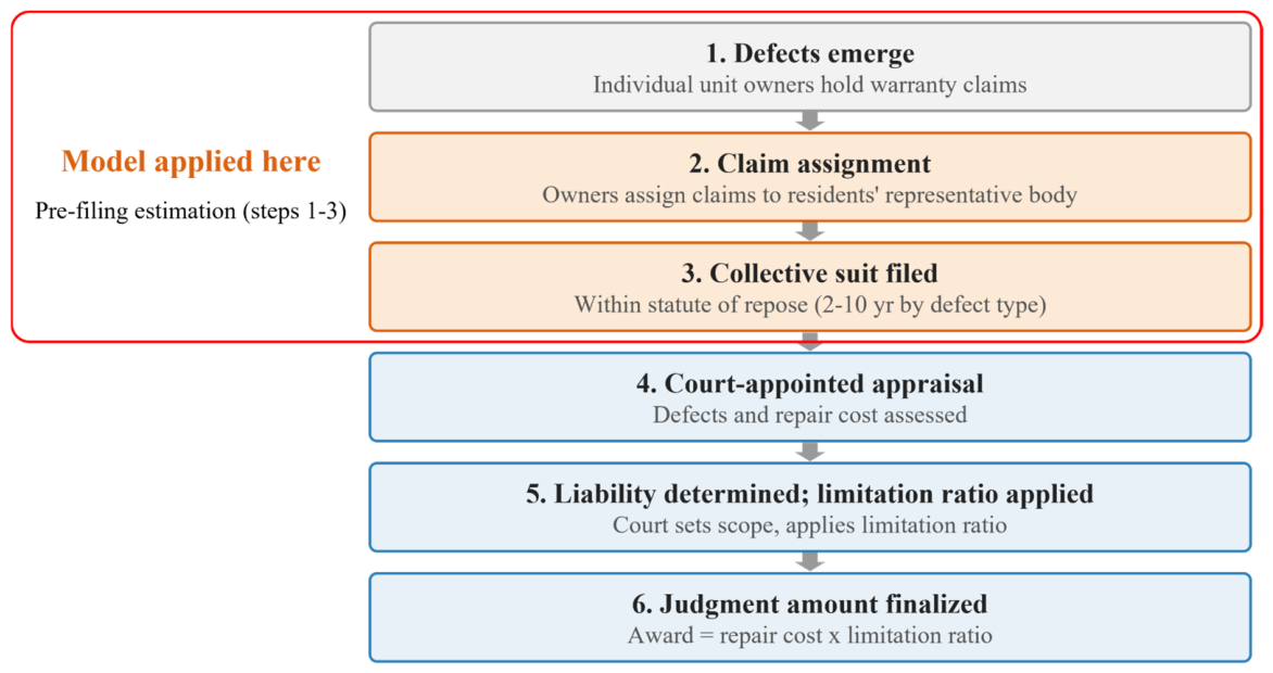
Because the institutional setting differs from common law jurisdictions, Figure 2 outlines the Korean multi-family housing defect litigation process. Individual unit owners first assign their warranty claims to the residents’ representative body, which files a single collective suit within the statute of repose. A court-appointed appraiser then assesses the defects and repair cost, after which the court determines the scope of liability and applies a liability limitation ratio reflecting the contractor’s defenses, yielding the final judgment amount. The proposed model operates before filing (steps 1–3), when only pre-litigation information is available.

3.2. Judgment Data Collection and Sample Screening

Judgment data were collected under four criteria: lawsuit type, building type, court instance, and time window. Lawsuit type was restricted to claims for damages in lieu of defect repair under Article 9 of the Act on Ownership and Management of Condominium Buildings and Article 667 of the Civil Act; unrelated suits (e.g., construction payment or unjust enrichment claims) were excluded. Building type was restricted to multi-family housing (apartment complexes) as defined under the Housing Act and the Enforcement Decree of the Building Act; non-residential facilities were excluded. Where a case proceeded to a higher instance, only the final instance judgment was retained as a statistical sample. Final instance status was determined from information identifiable at the time of collection. As is common for empirical studies based on publicly disclosed judgments, exhaustively tracing whether every first-instance judgment in the sample was later appealed is constrained by data accessibility, so the sample reflects the best available final instance determination as of collection. The collection window was approximately eleven years, covering judgments rendered between 2014 and 2025.

The window was limited to recent years for two reasons. First, contemporary validity; criteria for defect determination, appraisal practice, and liability limitation doctrine evolve over time, so a model intended to predict outcomes at the pre-filing stage must be calibrated to current judicial practice. Second, homogeneity and accessibility; the electronic disclosure of judgments and a standardized appendix format for defect cost schedules became common in this period, enabling consistent item-level extraction.

Judgment data were obtained from two sources, namely, archives held by defect-inspection firms and the Supreme Court of Korea judgment disclosure portal (portal.scourt.go.kr). After keyword-based first-pass filtering, each full text was read directly to confirm eligibility, the completeness of the judgment’s disposition (the operative ruling), and whether the itemized defect schedule could be extracted. Sample selection proceeded in three sequential stages, as follows: 156 judgments were initially collected; 37 non-multi-family-housing cases were excluded, leaving 119; and 13 intermediate instance judgments were excluded, yielding the final statistical sample of N = 106.

The 106 cases are balanced by region (Seoul metropolitan area 54 cases, 50.9%; non-metropolitan 52 cases, 49.1%). Cases involving large general contractors—defined here as firms ranked in the top 10 of the annual Construction Capability Evaluation [54]—account for 82 cases (77.4%), reflecting the market structure in which the construction of large multi-family housing complexes is concentrated among these major contractors. First-instance terminations dominate (99 cases, 93.4%), which provides practical justification for designing the model to estimate first-instance judgment amounts.

3.3. Variable Selection: Pre-Filing Availability

The design follows a single governing principle, namely, only information that both parties can independently verify before filing is admitted as an input variable. This follows directly from the model’s intended use, since the estimate informs decisions at the early dispute stage—when the decision to sue is being made—not after the outcome is fixed. Including post-hoc variables that are determined only at court appraisal would negate the model’s practical value.

Applying this principle yields three independent variables and two conversion-stage inputs. The three independent variables are elapsed months (months from the completion (use-approval) inspection—i.e., the regulatory approval for occupancy and use—to the field survey), log of total exclusive area (the sum of exclusive floor area across all households in the complex—i.e., private floor area excluding common areas, as registered in the building register; this registered figure excludes balconies and other service areas regardless of whether they have been enclosed through balcony extension), and log of claimed amount. Each of these is verifiable by both parties before a suit is filed. Elapsed months is fixed by the dates of the completion (use-approval) inspection and the field survey, both of which precede filing, and the total exclusive area is a registered physical attribute of the complex available from public property records. The claimed amount is set by the plaintiff at the point of filing and is therefore known at the decision-to-sue stage. Because judgments record only the plaintiff’s final pleaded amount, this variable reflects that final figure rather than the amount stated at initial filing; Section 6 discusses this limitation further. These three pre-filing variables are proxies for case scale and elapsed time, not for the case-specific legal findings—expert credibility, causation, contractual scope—that ultimately determine judicial outcome. The model is therefore not intended to substitute for legal assessment in factually atypical or legally contested cases.

The two conversion-stage inputs are the liability limitation ratio (predicted in Section 3.5) and the assigned claim exclusive area (measured before filing). Adding work-type cost shares was considered but rejected for three reasons. Such shares are post-hoc variables fixed only at court appraisal, and pre-filing private appraisal estimates diverge substantially from final court appraisals. Adding them would also induce multicollinearity with negligible R² gain. The variance inflation factors (VIF) of the three retained variables are all ≤ 2.46, which is well below the widely cited threshold of 10, though O’Brien cautions that such thresholds should not be applied mechanically [55].

3.4. Dependent Variable: Inflation Adjustment and Liability-Limitation Separation

Inflation adjustment. Because the cases span filing years 2014–2025, judgment amounts are deflated to a common scale using the Construction Cost Change Index (CCCI; 2020 = 100) [33], applied on the basis of the filing year rather than the judgment year. As filing precedes judgment, the relevant filing years extend to slightly earlier than the judgment window; over this period the index rose from 83.0 (2013) to 129.3 (2024).

Separation of the liability limitation ratio. Two identities hold across all 106 cases: the area-normalized judgment amount equals the judgment amount divided by the assigned-claim exclusive area, and the judgment amount equals the loss-compensation amount multiplied by the liability limitation ratio. Consequently, the area-normalized award is given by Equation (1),

$$area-normalized judgment={\displaystyle \frac{loss compensation\times liability limitation ratio}{assigned-claim exclusive area}}$$

(1)

If the area-normalized amount is used as the dependent variable and the liability limitation ratio is then multiplied again at the conversion stage, the ratio—already embedded in the numerator—is applied twice, under-predicting the actual judgment by an average of 24.0%. To remove this, the liability limitation ratio is separated out of the dependent variable and applied explicitly exactly once at the conversion stage. This is a deliberate normalization to eliminate an algebraic double-application, not a search for a new statistical relationship. It addresses the type of spurious correlation that arises when a ratio variable shares a common component across the dependent and conversion stages of an analysis [56]. The corrected dependent variable is defined in Equation (2),

$$log\left(loss-comp. per area, real\right)=log\left({\displaystyle \frac{area-normalized judgment}{liability limitation ratio\times (CCCI/100)}}\right)$$

(2)

We note that the resulting low correlation between the corrected dependent variable and the liability limitation ratio (r = 0.023, vs. 0.261 before separation) is partly an algebraic consequence of the definition. It is therefore reported only as a consistency check, not as statistical proof of independence; the justification for separation rests on the algebraic proof of double application above.

Robustness to dependent variable circularity. Because the dependent variable is normalized by area while area also enters as a regressor, one might suspect that R² is inflated by area appearing on both sides. To test this, an alternative model using the non-normalized total award (with only liability limitation and inflation separated) as the dependent variable was estimated under identical variables and folds. Its R² was higher (0.808 vs. 0.626), but this difference reflects the variance scale of the dependent variable, not predictive skill. Evaluated on the common basis of final-award prediction by five-fold cross-validation, the two models were essentially equivalent (MAPE 29.6% for the area-normalized model vs. 28.6% for the total-award model), and their quantile predictions (Q10–Q90) for a representative complex agreed within 5.1%. Moreover, the area coefficient of −0.875 is not an algebraic artifact. The dependent variable’s denominator (assigned-claim exclusive area) and the regressor (total exclusive area) are highly correlated but not identical (Spearman ρ = 0.991, Pearson r = 0.986). Substituting the denominator directly as the regressor yields a coefficient of −0.921, which does not converge to −1. Area normalization is therefore not a device that inflates R²; it is adopted for the interpretability of per-area unit cost and the consistency of liability separation, not for maximizing R².

The judgment amount itself includes both common area and exclusive area repair costs, averaging 59.7% common area share across the 106 cases. This share shows no significant relationship with complex size (Spearman ρ = 0.107, p = 0.28), so area normalization by V does not introduce a scale-dependent bias. Case-to-case variation in this share is instead absorbed within the residual heterogeneity captured by the prediction interval discussed in Section 3.6.

Dual role of elapsed months. Elapsed months are strongly negatively correlated with the liability limitation ratio (r = −0.891); as time passes, courts tend to narrow contractor liability owing to natural aging and maintenance lapses. After separation, the direct OLS coefficient of elapsed months is small (β = +0.0032); its substantive contribution instead emerges in the multinomial model (Section 3.5) as a predictor of the liability limitation band. Elapsed months thus play a dual role, namely, a direct regressor in the continuous model and a key predictor in the categorical model.

3.5. Model Architecture

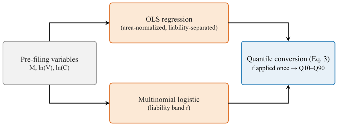
The model has a three-layer hybrid structure combining a continuous regression, a categorical classifier, and a quantile integration step (Figure 3).

(a) Area-normalized OLS regression. A log–log multiple regression estimates the corrected dependent variable from the three pre-filing variables. Log transformation is used because claimed and judgment amounts are right-skewed (improving residual normality after transformation) and because log–log coefficients are interpretable as elasticities. Coefficients are estimated with HC3 heteroskedasticity-robust standard errors. Stepwise entry confirmed the three-variable specification by AIC (detailed in Section 4.4). The final equation is Equation (3),

$${\hat{\mathrm{y}}}_B=8.1429+0.0032·M-0.8752·ln\left(V\right)+0.8095·ln\left(C\right)$$

(3)

where M = elapsed months, V = total exclusive area (m²), and C = claimed amount. The model yields R² = 0.626 (residual σ = 0.330). The area-elasticity of −0.875 reflects economies of scale; the claimed amount elasticity of +0.810 (<1) reflects a consistent judicial discount of the claimed amount (see Section 4.4). The model’s predictive performance is evaluated not by R² but by cross-validated MAPE and interval coverage (Section 3). Because all inputs are observable only before filing, coefficients are interpreted as predictive associations conditional on pre-filing information, not as causal effects.

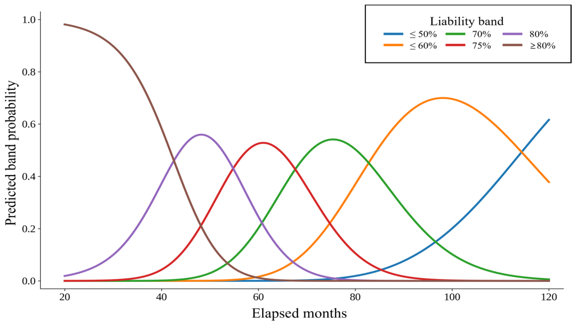
(b) Multinomial logistic classifier for the liability limitation band. A multinomial logistic regression, following the standard maximum-likelihood estimation procedure described in Hosmer et al. [19], predicts the probability that a case falls into each of six liability limitation bands. The predictors are elapsed months and years since completion—the litigation-filing year minus the completion-inspection year, an integer-valued case age measure distinct from the continuous elapsed-months variable. The model outputs band probabilities rather than a point ratio; the band-weighted mean is taken as the predicted ratio $\hat{\mathrm{r}}$. The predicted ratio declines monotonically from 85.5% at three years post completion to 58.5% at nine years.

(c) Probabilistic quantile integration. The two models are combined so that the liability limitation ratio is applied exactly once. The p-th quantile of the expected judgment is given by Equation (4),

$$Q_p=exp({\hat{\mathrm{y}}}_B+{\epsilon }_p)\times {\displaystyle \frac{{CCCI}_{filing-year}}{100}}\times \hat{r}\times {\displaystyle \frac{S_{assigned}}{\mathrm{10,000}}}$$

(4)

where ε_p is the p-th log-residual multiplier, $\hat{\mathrm{r}}$ is the predicted liability limitation ratio, and S_assigned is the assigned claim exclusive area (m², measured before filing). Using the measured assigned claim area directly—rather than decomposing it into area × assignment ratio—avoids accumulating rounding error and reflects the fact that this area is fixed during pre-filing consent collection. The OLS output (separated loss compensation—i.e., compensable damages before liability limitation) and the logistic output (liability ratio) each enter the equation only once, structurally preventing the double application error.

3.6. Quantile Multipliers via Leakage-Free Cross-Validation

The interval multipliers ε_p are derived by leakage-free five-fold cross-validation. In each fold, the OLS and multinomial models are trained on the training set (~85 cases) and used to predict the held-out validation set (~21 cases). The log of the ratio of actual to predicted judgment, log(actual/predicted), constitutes that fold’s log-residuals; the log-residuals from all five folds are pooled across the full 106 cases to form the empirical quantiles. Because only residuals from cases not used in training enter the calculation, interval underestimation due to overfitting is avoided.

The resulting multipliers are Q10 × 0.627, Q25 × 0.769, Q50 × 1.087, Q75 × 1.279 and Q90 × 1.447. The median multiplier of 1.087 (a modest ~8.7% upward correction) indicates small point-estimate bias. Q25 and Q75 (the interquartile range) are adopted as negotiation reference points because they span the central 50% of the predictive distribution. This is a standard choice, balancing wider intervals (e.g., Q10/Q90), which over-broaden the settlement range, against narrower ones (e.g., Q40/Q60), which are sensitive to sampling variation. A global multiplier is used; band-conditional multipliers are left to future work. At N = 106, splitting by elapsed-month bands leaves only 21–47 cases per band, making extreme-quantile multipliers depend on the top two to four observations and risking small-sample instability. The width of the Q10–Q90 interval is itself a statistical acknowledgment that cases similar in the three observed variables can diverge in judicial outcome due to legal factors not captured by the model (e.g., evidentiary disputes, contractual specifics). The interval should therefore be read as bounding this residual’s legal heterogeneity, not merely sampling variation.

3.7. Validation Procedure

Validity is assessed in two stages. Internal validity is evaluated by five-fold cross-validation (point MAPE and interval coverage), comparison against alternative models (Ridge, Random Forest, Gradient Boosting; results in Section 4.6), and time-ordered extrapolation. External validity is assessed on a separate set of judgments never used in training. The external sample comprises multi-family housing defect damages-in-lieu-of-repair lawsuits of the same type as the training sample (P001–P106), collected under the same criteria but not included in model fitting. Independence from the training set was verified by triple cross-checking (case number, total exclusive area, and complex name), yielding 22 independent cases. From each, only pre-filing variables were extracted; post-hoc variables such as appraisal amounts were excluded. Because the purpose is to evaluate pre-filing predictive performance, the liability limitation ratio for the external sample was not taken from the judgment, but predicted by the multinomial model from pre-filing variables (the same condition as internal cross-validation).

All statistical analyses were performed in Python (https://www.python.org/, accessed on 20 June 2026) using statsmodels (https://www.statsmodels.org, accessed on 20 June 2026) (OLS with HC3 robust standard errors; multinomial logistic regression), scikit-learn (https://scikit-learn.org, accessed on 20 June 2026) (five-fold and stratified K-fold cross-validation; benchmark models), and NumPy (https://numpy.org, accessed on 20 June 2026) (bootstrap, 2000 resamples, following the percentile method of Efron and Tibshirani [28]).

4. Analysis Results

4.1. Dispute Structure of the Sample

Across the 106 cases, the mean claimed amount was approximately USD 2.1 million and the mean awarded amount was approximately USD 1.3 million, with a mean first-instance litigation duration of 31.6 months (

Table 1. Descriptive statistics of case-level variables (N = 106).

Variable	Mean	Median	SD	Min	Max
Claimed amount (M USD)	2.15	1.86	1.43	0.23	7.28
Court-appraised (M USD)	1.94	1.61	1.36	0.23	7.33
Awarded amount (M USD)	1.33	1.12	0.89	0.14	4.57
Award ratio (%)	64.5	66.8	18.1	25.2	99.6
Liability limitation ratio (%)	76.0	80.0	9.1	40.0	90.0
Litigation duration (months)	31.6	30.5	9.4	15.0	66.0
Total exclusive area (1000 m2)	80.9	68.9	51.2	3.1	335.2
Assignment ratio (%)	93.8	95.7	6.5	61.4	100.0

Note: Top-10-ranked contractor cases 77.4%; metropolitan 50.9% (54/106); first-instance terminations 93.4%. Monetary amounts are in millions of U.S. dollars (M USD), converted from Korean won at approximately 1500 KRW per USD as of mid-2026.

)—indicating that the sample is weighted toward medium-to-large disputes. The award ratio (awarded ÷ claimed) averaged 64.5% with a large standard deviation (18.1 percentage points), whereas the liability limitation ratio averaged 76.0% with a much smaller standard deviation (9.1 percentage points). This contrast—high dispersion in the award ratio and low dispersion in the liability limitation—indicates that the uncertainty of the judgment amount arises mainly at the award ratio stage, while the liability limitation stage converges. This finding directly motivates the model architecture, in which a regression model explains award ratio variation and a separate classifier handles the convergent liability limitation band.

4.2. Two-Stage Deduction from Claim to Judgment

The judgment amount is reached through two structural deductions from the plaintiff’s claim. In all 106 cases (100%), the final award is smaller than the claim; the path from claim to judgment is therefore monotonically deductive. The mean total deduction was 35.5% of the claim, yielding the mean award ratio of 64.5% (

Table 2. Two-stage deduction from claim to judgment (N = 106).

Stage	Mechanism	Mean Deduction	Mean (M USD)	Ratio to Claim
1. Claimed	private appraisal	-	2.15	100.0%
2. First deduction	claim -> loss comp.	14.3 pp	-	-
3. Court appraised	appraiser	-	1.94	-
4. Second deduction	liability limitation	24.0 pp	-	-
5. Awarded	final judgment	35.5 pp total	1.33	64.5%

Note: First-deduction SD 25.1 pp; second-deduction SD 9.1 pp; baseline conversion 64.5% × 76.0% = 49.05%. Monetary amounts are in millions of U.S. dollars (M USD), converted from Korean won at approximately 1500 KRW per USD as of mid-2026.

).

The internal structure of the first-stage deduction (claim → loss compensation) is not simple: it averages 14.3 percentage points but with a very large standard deviation (25.1 percentage points), including negative values (minimum −45.5 percentage points). Court-appraised amounts are lower than claimed in 62 cases (58.5%)—of which 30 cases (28.3%) are over-claims exceeding 1.25× the appraised amount—but exceeds the claim in 44 cases (41.5%), reflecting conservative private appraisals or defects recognized only during court appraisal. The first stage thus mixes over-claiming (information asymmetry) and private-appraisal under-estimation.

The second-stage deduction (loss compensation → judgment) averages 24.0 percentage points with a much smaller standard deviation (9.1 percentage points), driven by the application of the liability limitation ratio (mean 76.0%). That the second-stage dispersion is less than half the first-stage dispersion indicates that liability-limitation application follows a far more consistent judicial pattern than the claim/appraisal stage. This asymmetry of variances is the direct basis for separating the model into a regression component (award ratio variation) and a classification component (liability limitation band). Combining the two mean parameters gives a baseline conversion ratio of 64.5% × 76.0% ≈ 49.05%. This is a simple approximation that assumes the award ratio and the liability limitation ratio are independent; it serves only as an intuitive starting point (“roughly half of the claim is awarded”) that the probabilistic quantile model refines case by case.

4.3. Liability Limitation Distribution: Judicial Standardization

The liability limitation ratio showed pronounced banded concentration (mean 76.0%, median 80.0%, SD 9.1 pp) (

Table 3. Distribution of the liability limitation ratio by band (N = 106).

Band	Liability Ratio	Cases	Share/Cumulative
1	<50%	3	2.8%/2.8%
2	50–60%	6	5.7%/8.5%
3	60–70%	23	21.7%/30.2%
4	70–75%	17	16.0%/46.2%
5	75–80%	29	27.4%/73.6%
6	>80%	28	26.4%/100.0%
3–5	60–80% combined	69	65.1%

Note: Mean 76.0%, median 80.0%, SD 9.1 pp; early 72.7% vs. recent 78.9% (p < 0.05).

). Three adjacent bands—60–70% (23 cases, 21.7%), 70–75% (17 cases, 16.0%), and 75–80% (29 cases, 27.4%)—together account for 69 cases (65.1%), with the 75–80% band the single most frequent and its mode coinciding with the median. A further band above 80% (28 cases, 26.4%) forms a second concentration. This convergence toward the 60–80% range indicates a judicial standardization in which courts apply liability limitation within a narrow, quasi-standard range. The liability limitation itself reflects the principle of the equitable apportionment of loss, by which courts allocate a share of the damage to factors beyond the contractor’s control—such as natural aging, residents’ use, and maintenance lapses. Because the determination converges within a limited range, band-level prediction (rather than exact-ratio prediction) is feasible—the methodological premise of the multinomial classifier. The liability ratio also rose over time (early 2013–2018 cases—72.7%; recent 2019–2023 cases—78.9%; difference 6.2 pp, Mann–Whitney p < 0.05), motivating the inclusion of a time-related predictor.

4.4. Area-Normalized OLS Regression

The final OLS model (Equation (3)) explained the corrected dependent variable with R² = 0.626 (adjusted R² = 0.615; residual σ = 0.330) (

Table 4. Final OLS regression coefficients (HC3 robust SE, N = 106).

Variable	Coef. (β)	SE (HC3)	t	p	95% CI
Constant	+8.1429	0.6186	13.16	<0.001	[6.930, 9.355]
Elapsed months	+0.0032	0.0018	1.75	0.080	[−0.000, 0.007]
log(area)	−0.8752	0.0731	−11.97	<0.001	[−1.019, −0.732]
log(claim)	+0.8095	0.0750	10.79	<0.001	[0.662, 0.957]

Note: DV = log(area-normalized award/liability ratio/(CCCI/100)). R² = 0.626; σ = 0.330; VIF ≤ 2.46.

). The area elasticity (β = −0.875) reflects economies of scale: a 1% increase in exclusive area is associated with a 0.875% decrease in loss compensation per unit area, an almost proportional decline. The claimed-amount elasticity (β = +0.810, <1) reflects a consistent judicial discount—each 1% increase in the claim translates into only a 0.810% increase in per-area compensation. The elapsed-months coefficient is small and not significant at the 5% level (β = +0.0032, p = 0.080) after liability-limitation separation; its substantive role appears instead in the classifier (Section 3.5). Residual diagnostics indicated approximate normality after log transformation (skewness −0.573, kurtosis −0.589) and homoskedasticity across liability bands (Levene F = 0.309, p = 0.907). Chow tests for structural stability were non-significant for both contractor size (F = 1.66, p = 0.166) and region (F = 1.84, p = 0.128), indicating the three-variable model applies across these subgroups without separate calibration.

Table 5. Stepwise OLS specification (corrected vs. uncorrected, N = 106).

Model	Variables	R2 (Corr.)	Adj. R2	R2 (Uncorr.)	AIC
M1	elapsed months	0.026	0.017	0.137	167.23
M2	log(area)	0.133	0.125	0.158	154.92
M3	log(claim)	0.040	0.031	0.038	165.72
M4	elapsed months + log(area)	0.145	0.128	0.256	155.48
M5	elapsed months + log(claim)	0.061	0.042	0.162	165.43
M6	log(area) + log(claim)	0.613	0.605	0.678	71.49
M7	all three	0.626	0.615	0.686	69.78

Note: M7 minimizes AIC. AIC is computed using the corrected-DV (liability limitation separated) model for all rows.

reports the stepwise progression to this specification.

Heteroskedasticity was examined further in the elapsed month dimension. Partitioning the sample into three elapsed month groups (≤36, 37–60, and ≥61 months) did not reject the equality of residual variances (Levene W = 1.42, p = 0.25; for the six liability bands, Levene F = 0.31, p = 0.91). However, the cumulative MAPE rose with elapsed months, from about 21% for the youngest group to about 34% for the oldest. A weak monotonic association was also found between elapsed months and squared log-residuals (Spearman ρ = 0.249, p = 0.010), indicating that predictive uncertainty increases somewhat for older complexes. Because the model applies a single global set of residual-quantile multipliers, its prediction intervals may slightly under-represent the true variability for complexes older than about 61 months; this is noted as a limitation. HC3 robust standard errors were nonetheless used at the coefficient estimation stage to preserve efficiency in the presence of any heteroskedasticity. The prediction intervals are built nonparametrically from empirical residual quantiles, so their validity does not rely on a parametric normality assumption.

As explained in Section 3.6, the use of a single global multiplier rather than elapsed-month-conditional multipliers is a deliberate design choice, not an oversight of this heteroskedasticity. At N = 106, partitioning by the elapsed month band leaves only 21–47 cases per band, too few to estimate extreme quantiles (e.g., Q10, Q90) without the result depending on the top two to four observations. The finding here quantifies the resulting calibration cost more precisely, and motivates the time-stratified multipliers left to future work with a larger sample.

Because all inputs are observable only before filing, the coefficients are interpreted as predictive associations conditional on pre-filing information rather than causal effects. A two-variable model excluding the claimed amount (elapsed months and log area only) yielded R² = 0.145 and a five-fold MAPE of 42.4%, versus R² = 0.626 and MAPE 29.6% for the three-variable model. This confirms that the claimed amount is the most informative pre-filing signal of case scale, justifying its inclusion for a predictive (not causal) objective. 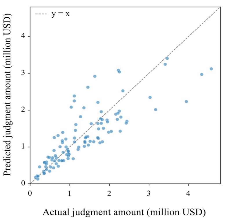Figure 4 plots predicted against actual judgment amounts for the training sample.

4.5. Multinomial Logistic Classifier for the Liability Limitation Band

The multinomial logistic model predicts the probability of each of six liability limitation bands from elapsed months and years-since-completion. In five-fold cross-validation, the ±1-band tolerance accuracy was 94.4%, confirming that band-level prediction is reliable even though exact ratio prediction is not (

Table 6. Multinomial logistic classifier performance (5-fold CV, N = 106).

Metric	Performance	Interpretation
Exact-band accuracy	61.3% ± 12.2 pp	Correct band among 6
±1-band accuracy	94.4% ± 3.5 pp	Adjacent band included
Predictors	elapsed months, years-since-completion	Pre-filing only

Note: StratifiedKFold; the high SD of exact accuracy reflects the small lowest-frequency band.

). The band-weighted predicted ratio declined monotonically with time, from 85.5% at three years post-completion to 58.5% at nine years (Figure 5). This is consistent with courts narrowing contractor liability as buildings age.

Because the liability limitation bands are concentrated in the 70–80% range (69 of 106 cases, 65.1%), the classifier’s accuracy is interpreted against a no-information baseline that assigns every case to the modal band. That baseline attains 27.4% exact-band and 69.8% ±1-band accuracy, whereas the model attains 61.3% and 94.4%, exceeding the baseline by 33.9 and 24.6 percentage points, respectively. The model therefore provides discriminative information beyond the sample’s class imbalance, rather than merely defaulting to the majority band. Even for the sparse low-liability bands (≤50% and 50–60%, N = 9), the ±1-band accuracy remains 88.9%, indicating that the classifier retains resolution for the contractor-favorable cases that are rare in the sample. The lowest-frequency band (50–60%, N = 6) is best used as a probability distribution over adjacent bands rather than as a point prediction.

4.6. Integrated Model: Cross-Validation and Calibration

Under leakage-free five-fold cross-validation, the integrated quantile model achieved a median prediction (Q50) MAPE of 28.4% (±4.8 pp across folds) (

Table 7. (a) Integrated model cross-validation performance (5-fold, N = 106). (b) Benchmark comparison (area-normalized stage MAPE).

(a)
Metric		Performance
Q50 MAPE		28.4% ± 4.8 pp
50% coverage (Q25–Q75)		49.1% (nominal 50%)
80% coverage (Q10–Q90)		79.2% (nominal 80%)
Cases outside 80% interval		22 (20.8%)
(b)
Model	MAPE	SD	Note
OLS (this study)	29.6%	-	best, interpretable
Ridge	29.7%	-	approx OLS
Random Forest	39.0%	±12.0 pp	overfits
Gradient Boosting	41.2%	±13.2 pp	overfits

Note: Integrated MAPE (28.4%) and area-normalized stage MAPE (29.6%) differ by computation stage. SD is omitted for OLS and Ridge because these estimators are deterministic given the fold partition, and therefore have no across-run sampling variability to report. 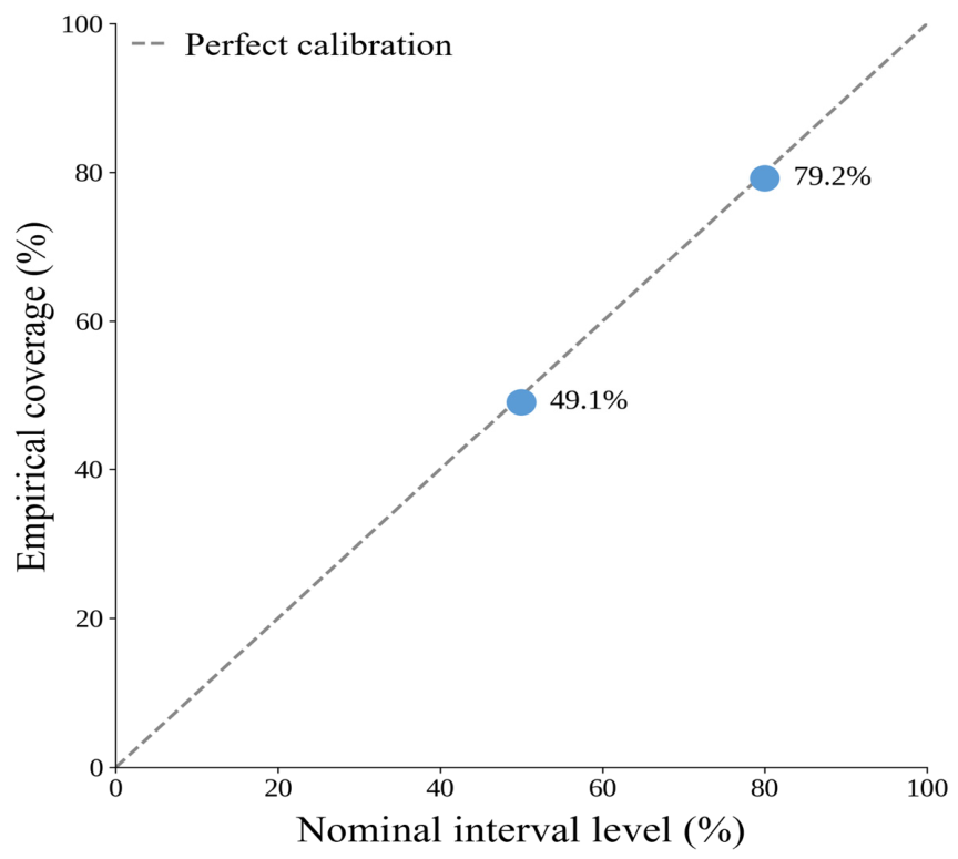Random Forest and Gradient Boosting, by contrast, involve stochastic components (bootstrap resampling, feature subsampling), so their SD reflects variability across repeated fits.

a). More importantly for a model that outputs intervals, the empirical coverage closely matched nominal levels. The 50% prediction interval (Q25–Q75) covered 49.1% of actual judgments, and the 80% interval (Q10–Q90) covered 79.2% (Figure 6). This near-nominal coverage indicates the prediction intervals are properly calibrated. A point estimate carrying ±30% error while the interval estimate meets its nominal confidence level supports the model’s intended use as a negotiation band tool rather than a single point predictor. The small between-fold variation (MAPE SD 4.8 pp) indicates the model does not depend heavily on a particular split.

The OLS-based specification was benchmarked against regularized and ensemble alternatives under identical variables and folds. The OLS model (MAPE 29.6%) and Ridge regression (29.7%) were essentially equivalent, indicating little room for improvement via regularization. Tree ensembles, by contrast, performed substantially worse (Random Forest 39.0%, Gradient Boosting 41.2%) (Table 7b). At N = 106, complex nonlinear models overfit, while the log-linear structure of the relationship favors the simple, interpretable linear model. A time-ordered cumulative split (training 60 → 90%, predicting later years) yielded a MAPE of 34.6%, higher than the random five-fold result—reflecting the construction cost surge of 2021–2022 and the inherent difficulty of forward prediction. Even so, this remains well below a naïve mean baseline, and suggests periodic re-training on recent data in practice.

4.7. Preliminary External Validation

The model was applied to 22 independent judgments never used in training—multi-family housing defect damages-in-lieu-of-repair lawsuits of the same type as the training sample—verified as non-overlapping with the training set by triple cross-checking (case number, total exclusive area, complex name). Only pre-filing variables were extracted; post-hoc variables were excluded. To evaluate genuine pre-filing performance, the liability limitation ratio was not read from the judgment but predicted by the multinomial model. The ±1-band accuracy on the external sample was 95.5%, consistent with the internal cross-validation accuracy (94.4%).

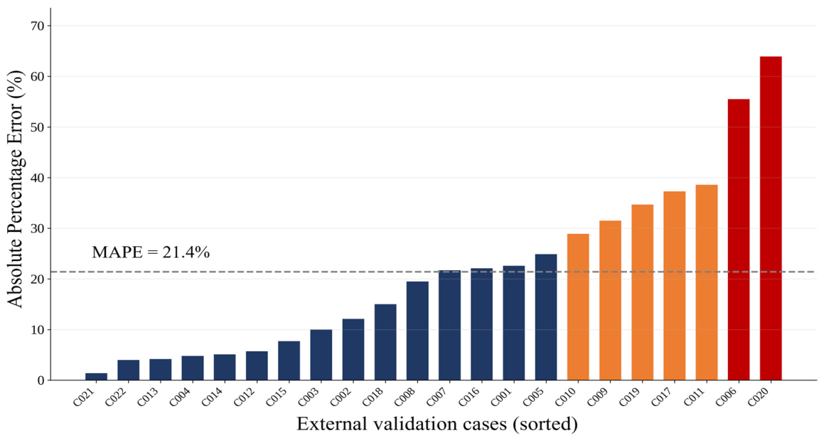
Using the predicted liability ratio, the cumulative MAPE was 21.4% (median 20.6%), with a bootstrap (2000-resample) 95% confidence interval of [15.0%, 28.6%] (

Table 8. Preliminary external validation sample and performance (N = 22).

Item	Value	Note
External sample	22 cases	Same type; non-overlapping
MAPE (predicted r-hat)	21.4% (median 20.6%)	Same condition as internal
MAPE (observed r-hat)	19.2%	Reference only
MAPE (uniform mean 75.7%)	23.4%	Baseline
Bootstrap 95% CI	[15.0%, 28.6%]	2000 resamples
±1-band accuracy	95.5%	vs. internal 94.4%
Q10–Q90 coverage	82% (18/22)	vs. internal 79.2%
Q25–Q75 coverage	59% (13/22)	vs. internal 49.1%

Note: External cases anonymized C001–C022; pre-filing variables only.

). This lies between the result using the observed liability ratio (MAPE 19.2%) and a baseline applying the mean ratio (75.7%) uniformly (MAPE 23.4%; this uniform-ratio baseline error is unrelated to the 24.0 pp second-stage deduction reported in Section 4.2). The predicted ratio thus achieved 2.0 pp lower error than uniform application, confirming the practical contribution of the classifier. Residual quantile coverage was 82% (18/22) for Q10–Q90 and 59% (13/22) for Q25–Q75, consistent with the internal coverage (79.2% and 49.1%) (Figure 7). Of the 22 cases, 16 had errors below 30%; the three largest errors (C020, C006, C011) corresponded to complexes whose per-area judgment structure lay at the edge of the training distribution.

That the external MAPE (21.4%) under predicted liability limitation was lower than the internal cross-validation MAPE (28.4%)—both computed under the same predicted ratio condition—suggests no clear sign of overfitting to the training sample. However, the external sample (n = 22) is small, and its bootstrap interval is wide. The external sample’s key predictors (log area, log claim) also have smaller standard deviations than the training sample (0.71 → 0.56 and 0.71 → 0.58), so its distribution is relatively concentrated in the central region of the training data. The mean leverage of the external sample ($\overline{\mathrm{h}}$* = 0.038) is, however, essentially equal to that of the training sample ($\overline{\mathrm{h}}$ = 0.038). We therefore interpret this result not as direct proof of the absence of overfitting, but as supporting evidence that the model operates stably on unseen cases without clear signs of overfitting.

5. Discussion

5.1. Interpretation in the Light of Previous Works

The model’s central result is a calibrated probabilistic interval estimated from only three pre-filing variables. This addresses the gap identified across Section 2.2, Section 2.3 and Section 2.4: to our knowledge, no prior study in this literature combines pre-filing restriction, continuous interval estimation, and external validation.

Two findings deserve emphasis. First, the variance asymmetry between the award ratio (SD 18.1 pp) and the liability limitation ratio (SD 9.1 pp) is not merely descriptive; it is the structural reason the hybrid architecture works. Because liability limitation converges toward a narrow 60–80% band (judicial standardization), it can be predicted at the band level with high tolerance accuracy (±1-band 94.4%), while the more variable award magnitude is left to the continuous regression. Treating these two sources of variation with a single model would conflate a convergent judicial pattern with a dispersed economic one. Second, the near-nominal interval coverage (49.1% and 79.2% against nominal 50% and 80%) indicates that the value of the model lies less in its point accuracy (MAPE ≈ 28%). Rather, its value lies in the statistical validity of the intervals it produces—which is precisely what a negotiation tool requires. Accordingly, the model’s value lies in providing a baseline reference for the ordinary run of cases, not a substitute for case-specific legal analysis in outlier disputes.

The point error (MAPE 28.4%) and the width of the negotiation interval answer different questions and should not be conflated. Relative to the median (Q50), Q25 sits at 70.7% and Q75 at 117.7% of Q50—a band of roughly −29% to +18% around the central estimate, narrower than the raw MAPE figure might suggest. This band is not benchmarked against a hypothetical perfect predictor but against the status quo, in which neither party has any objective estimate at all. A bounded, calibrated range is an improvement over that baseline regardless of its absolute width.

5.2. Practical Use: A Shared Reference for Both Parties

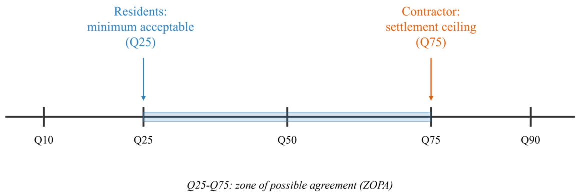
The single estimate resolves two parties’ distinct decisions simultaneously, with each party’s litigation alternative—its best alternative to a negotiated agreement (BATNA)—setting its reservation point. From the contractor’s perspective, the upper quartile (Q75) functions as a reasonable settlement ceiling: proceeding to judgment carries roughly a 25% probability of an award exceeding Q75, so a settlement at or below Q75 is preferable to bearing that downside risk in court. From the residents’ perspective, the lower quartile (Q25) is the minimum acceptable settlement: an offer below Q25 is worse than the roughly 75% probability of recovering more than Q25 through litigation. Because the contractor will rationally settle at or below Q75 and the residents will rationally settle at or above Q25, the interquartile band (Q25–Q75) defines a non-empty zone of possible agreement that both parties can share before filing (Figure 8). This addresses the missing condition—the visibility of economic incentives—that weakens existing alternative dispute-resolution mechanisms. Because litigation in the sample averaged 31.6 months, the time value of an earlier settlement further widens this zone around the median (Q50). This shared-reference function is the model’s principal practical contribution; its detailed translation into stage-by-stage prevention and response strategies for each party is left to a separate study. Realizing this contribution in practice depends on adoption incentives that lie outside the model itself. Plaintiff-side counsel compensated on a contingency basis, for instance, may resist a conservative estimate, and courts do not formally recognize such tools. The model is therefore positioned as a voluntary pre-filing reference for the parties rather than an instrument with evidentiary standing. How each stakeholder would adopt it in routine practice, however, is left to future study.

One concern for any decision-support tool that uses the claimed amount as an input is strategic manipulation (a Goodhart-type effect): a party aware of the model might inflate the claim to shift the estimate. Two features limit this risk. First, the claimed-amount elasticity is below one (β = 0.810), so inflating the claim yields a less-than-proportional change in the estimate. A 10%, 20%, or 30% increase in the claim, for example, raises the predicted judgment by only about 8.0%, 15.9%, and 23.7%, respectively, providing partial built-in damping. Second, the claimed amount in practice is not a free parameter but is anchored by the plaintiff’s private appraisal and by the assignment-based collective-action structure, which constrains arbitrary inflation. For operational use, we nonetheless recommend that the claimed amount entered into the model be bounded by an independently verifiable basis (e.g., a documented private appraisal) to further reduce manipulation incentives.

The claimed amount’s centrality to predictive performance also invites a broader question: does the model estimate defect severity, or merely the plaintiff’s stated position? In practice, the claimed amount is not a purely strategic figure. It is itself derived from a private technical appraisal conducted before filing—an engineering assessment of defect scope and repair cost commissioned by the residents’ representative body—so its predictive contribution reflects, at least in part, pre-suit engineering information rather than unconstrained litigation strategy. This also clarifies why the three-layer architecture, rather than a simple percentage-of-claim heuristic, is needed. The claimed amount alone does not resolve the liability limitation band—which the multinomial classifier predicts separately with ±1-band accuracy of 94.4%, and which is the primary source of dispersion the contractor’s defenses introduce. Nor does it yield a calibrated prediction interval, which the quantile layer provides. The model’s contribution therefore lies in decomposing a single reported figure into an engineering-grounded scale component, a legally determined liability discount, and a statistically calibrated uncertainty band—not in substituting the claimed amount for engineering judgment.

The dispersion between the claimed amount and the court-appraised amount further supports this reading (SD 28.1 pp across the 106 cases; distinct from the claim-to-loss-compensation dispersion reported in Table 2). This dispersion includes 44 cases in which the court appraisal exceeded the claim. If claimants simply adopted the appraised figure after the fact, this dispersion would not arise. Nor would the sub-unity claimed-amount elasticity (β = 0.810) reported in Section 4.4. The claimed amount instead reflects the plaintiff’s own pre-filing assessment, anchored in a private technical appraisal that the plaintiff may or may not later reconcile with the court’s finding. This anchoring is also institutionally required. Because claim assignment litigation depends on individual owners voluntarily assigning their claims to the residents’ representative body—at a mean assignment rate of 93.8% in our sample—the representative body must present an expected recovery figure to secure that assignment. This figure is grounded in the private appraisal, reinforcing the claimed amount’s pre-filing origin.

A related equity concern arises primarily from contractor size composition. Because the model is calibrated on cases weighted toward large, top-10-ranked contractors (77.4%; Table 1), its estimates may be less reliable—and should therefore be applied more cautiously—for disputes involving smaller contractors, where the training data are comparatively thin. Regional composition is, by contrast, comparatively balanced (Seoul metropolitan area 50.9% vs. non-metropolitan 49.1%; Table 1). This concern is therefore less pronounced across regions, though some caution remains warranted given the modest overall sample size.

6. Conclusions

Disputes over defects in multi-family housing impose a substantial social cost. Yet at the moment the decision to sue is made, neither contractors nor residents can objectively foresee the likely judgment amount; this information asymmetry entrenches over-claiming, prolonged litigation, and adversarial compensation over substantive repair. To address this, the present study set out to develop and validate a model that estimates the expected judgment amount using only variables available before a suit is filed. Both parties, in this way, may share an objective reference at the pre-litigation stage.

Using a dataset of 106 final-instance Korean judgments (2014–2025), decomposed into 33,997 item-level records, a three-layer hybrid model was constructed. This comprised an OLS regression of the area-normalized award on three pre-filing variables (R² = 0.626), a multinomial logistic classifier predicting the liability limitation band (±1-band accuracy 94.4%), and a probabilistic quantile layer. Under leakage-free five-fold cross-validation, the model achieved a median MAPE of 28.4% with well-calibrated prediction intervals (49.1% and 79.2% coverage against nominal 50% and 80% levels). A preliminary external validation on 22 independent cases yielded a MAPE of 21.4% with no clear sign of overfitting.

These results directly answer the study’s two research questions: RQ1 is answered affirmatively by the calibrated interval performance reported above, and RQ2 is answered affirmatively by the external validation result, which showed no clear sign of overfitting.

Academically, the study makes three contributions. It provides a pre-litigation estimation model that, unlike prior work dependent on post-hoc variables, relies solely on information available before filing. It introduces a deliberate separation of the liability limitation ratio that corrects an algebraic double application error, and it adds an independent external validation that prior studies in this area generally did not report, strengthening confidence in the model’s generalizability.

Practically, the single estimate serves both parties’ distinct decisions. The lower quartile (Q25) functions as a conservative recovery floor for residents, and the upper quartile (Q75) as a conservative loss ceiling for contractors, so that the interquartile band (Q25–Q75) defines an objective zone of possible agreement before filing. By making the economic incentives of litigation visible in advance, the model offers a shared reference that can shift defect disputes from adversarial compensation toward earlier, information-based settlement.

These findings are subject to several limitations. The sample is concentrated in top-10-ranked contractors and the metropolitan area—reflecting the structure of Korea’s housing-construction market—and is restricted to claim-assignment-based collective litigation. Relatedly, because the dataset comprises only cases that proceeded to final judgment, defect disputes resolved earlier by settlement are not represented. This constitutes a form of sample selection bias: cases resolved through early settlement—plausibly those with less severe or less contested defects—are systematically absent from the training data. Coefficients estimated on adjudicated cases may not generalize to the settled population. The estimate therefore reflects the expected adjudicated outcome conditional on litigation, and should be read as an upper reference point for the litigation alternative rather than as a normative settlement price.

A related limitation concerns the temporal status of the claimed amount itself. Under Korean civil procedure, an initial complaint must state a definite claim amount, but plaintiffs in defect repair suits commonly file an explicit partial claim and formally expand it once the court-appointed appraisal is completed. Because judgments record only the final pleaded amount, the claimed amount variable used here reflects this post-expansion figure rather than the amount stated at initial filing. The frequency of such amendments cannot be determined from judgment text alone, since only exceptional cases—typically involving a statute-of-repose objection to the expanded portion—record the pre-expansion figure. This final figure is itself often contested: plaintiffs formally objected to the court-appointed appraisal in 90 of the 106 cases (84.9%), commonly amending their claim upward rather than adopting the appraiser’s figure outright. The claimed amount therefore retains an independent, plaintiff-driven component beyond the court appraisal. This is precisely why the model is designed to output a probabilistic interval rather than a single point estimate; the interval is intended to absorb this input uncertainty, together with the residual legal heterogeneity discussed in Section 3.6.

The integrated error (MAPE 28.4%) implies that the model should be used as an interval estimate rather than a single point. Moreover, because all inputs are observable only before filing and no instrumental variable is available, the coefficients are interpreted as predictive associations rather than causal effects.

The external validation, moreover, remains preliminary given its small sample (n = 22): the bootstrap 95% confidence interval for the external MAPE ([15.0%, 28.6%]) reflects this sampling uncertainty. The largest external validation errors, moreover, occurred for cases whose per-area judgment structure lay at the edge of the training distribution, so the model’s output should be treated with additional caution for such profiles. Formal sample size criteria for developing and externally validating multivariable prediction models with a continuous outcome have been proposed in the literature [57,58]. By these benchmarks, both the development sample (N = 106) and the external validation sample (N = 22) used here are modest.

Future research should expand and diversify the external validation sample beyond the dominant segments, and explore instrumental variable approaches should a valid instrument for the claimed amount be identified. It should also establish, through longitudinal or quasi-experimental designs, whether defect-prevention measures causally reduce judgment amounts.