Coupling Mechanisms Between Spatial Adaptability and Embodied Carbon Emissions in Residential Buildings: Identifying an Upper Fixed-Wall-Ratio Threshold Through Dynamic Life-Cycle Scenarios

Abstract

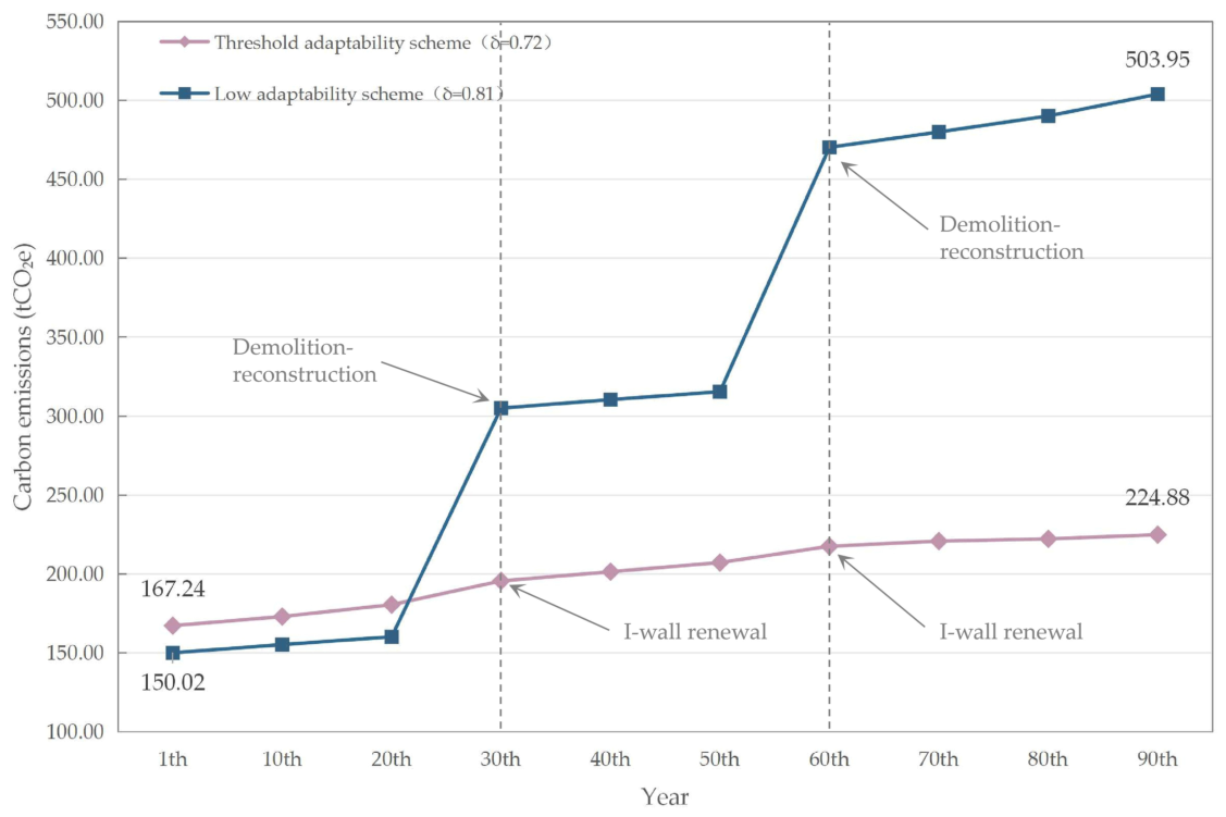
The aim of this study is to identify, through layout-coverage testing, the upper fixed-wall ratio at which the reconfigurable layout set can still fully satisfy mainstream spatial demand, and to quantify, under consistent structural, temporal, and accounting conditions, how 90-year cumulative embodied carbon emissions change across δ scenarios and how crossing this threshold alters the residential update pathway. A design-sample database of 954 residential floor plans was used to develop a common “basic unit,” and a wall-based index, δ, was defined as the ratio of fixed-wall length to total interior-wall length. A multiple-response survey of 168 households was then used to establish a mainstream layout set; layouts were ranked by selection frequency, and the smallest ranked set whose cumulative share exceeded 50% of all selections was retained. Eleven δ scenarios were assessed over a potential 90-year service-life scenario that incorporated interior reconfiguration, I-wall renewal, and possible demolition–reconstruction. The results identify δ ≈ 0.72 as the upper fixed-wall-ratio threshold compatible with full coverage of the mainstream layout set. When δ ≤ 0.72, internal reconfiguration maintains mainstream-layout coverage, and cumulative embodied carbon ranges from 224.88 to 313.46 tCO₂e, equivalent to 1772.10–2470.13 kgCO₂e/m². When δ > 0.72, at least one mainstream layout becomes infeasible and the modeled update pathway shifts to demolition–reconstruction, increasing emissions to 402.62–503.95 tCO₂e, or 3172.73–3971.24 kgCO₂e/m². Dynamic trajectories for the representative δ = 0.72 and δ = 0.81 scenarios show that the former accumulates emissions gradually, with limited increases associated with I-wall renewal at Years 30 and 60, whereas the latter undergoes sharp jumps at the same nodes because insufficient layout coverage triggers demolition–reconstruction. These findings provide an operational basis for using the fixed-wall ratio as an early-stage carbon-screening variable while retaining the need for project-specific multi-performance verification.

1. Introduction

Whole-life carbon assessment has increasingly shifted from an almost exclusive focus on operational energy to the material- and process-related emissions embodied in buildings [1,2,3,4,5,6,7]. Embodied carbon was historically less visible in design and policy because operational energy was directly measurable during use, whereas material-related emissions were distributed across supply chains, construction activities, replacement cycles, and end-of-life processes. Recent renovation research shows that excluding embodied carbon can distort comparisons between retention, renovation, and new construction, particularly when the retention of existing fabric avoids substantial new material inputs [8]. Because structural layout, material quantities, and the degree of spatial fixedness are largely locked in during concept design, embodied carbon and future adaptability should be considered before these decisions become costly or impossible to reverse. Comparative life-cycle studies show that service-life extension, renovation, and avoided reconstruction can reduce annualized or cumulative embodied carbon [9,10,11,12,13,14,15,16,17], although the magnitude is sensitive to service-life assumptions, replacement cycles, system boundaries, and end-of-life treatment. Against this background, the present study focuses on identifying a measurable spatial-design condition that can prevent carbon-intensive reconstruction under changing residential demand.

Research on residential obsolescence identifies a persistent mismatch between long structural lives and shorter functional lives. When household composition, living patterns, building services, or spatial requirements change, a rigid interior organization can shift the response from local reconfiguration to invasive renovation or premature demolition [18,19,20,21,22,23,24,25]. This sequence shortens functional service life, generates repeated material input and construction waste, and causes embodied carbon to accumulate even when the primary structure remains physically serviceable. Studies of demolition and construction waste further quantify the associated resource loss and low recovery performance [26,27,28,29]. Nevertheless, service life is commonly treated as an external scenario assumption rather than as an outcome partly conditioned by the dwelling’s capacity to accommodate changing demand. The causal mechanism linking spatial inflexibility, update decisions, and embodied-carbon accumulation therefore remains insufficiently specified.

Open Building, SI housing, and SAR housing address this problem by separating long-life support systems from replaceable infill systems [30,31,32,33,34,35,36]. Related studies evaluate adaptable partitions, reversible connections, modular construction, design for disassembly, and component reuse through case comparison, material-flow analysis, or life-cycle assessment [37,38,39,40,41,42,43,44,45,46,47,48,49,50,51,52]. These studies generally demonstrate that reversible and reusable components can reduce waste and embodied impacts. Their results, however, are often specific to a particular technology or case, and adaptability is frequently represented by qualitative design principles, reuse rates, or disassembly potential rather than by an occupant-demand-based spatial threshold.

A parallel methodological stream has introduced scenario-based and dynamic life-cycle assessment to represent time-dependent replacement, renovation, and carbon factors [53,54,55,56,57,58,59], while layout-adaptability research has developed graph-based measures of spatial generality and change potential [60]. These approaches improve temporal or spatial representation, respectively, but they are rarely integrated. In particular, existing studies seldom convert household preferences into an explicit layout-coverage requirement, identify the maximum degree of spatial fixedness compatible with that requirement, and then quantify the carbon consequence of crossing the resulting threshold. This unresolved integration constitutes the principal research gap addressed here.

The distinction between a transferable method and context-specific numerical inputs is especially important internationally. In the European Union, the Level(s) framework provides a common life-cycle global-warming-potential indicator for residential and office buildings, while national environmental product declarations, life-cycle inventory databases, transport conditions, and end-of-life practices remain relevant to calculation outcomes [61,62]. In India, building LCA studies likewise emphasize the need for regional and temporal inventories, and the India Construction Materials Database was developed to provide market-appropriate data for commonly used materials [63,64]. Accordingly, the wall-classification, layout-coverage, and event-based assessment procedure developed here can be transferred across markets, but the candidate layout set, feasibility constraints, emission factors, transport distances, recovery assumptions, and numerical carbon totals must be recalibrated locally.

Accordingly, the aim of this study is to identify, through layout-coverage testing, the upper fixed-wall ratio at which the reconfigurable layout set can still fully satisfy mainstream spatial demand, and to quantify, under consistent structural, temporal, and accounting conditions, how 90-year cumulative embodied carbon emissions change across δ scenarios and how crossing this threshold alters the residential update pathway. The analysis addresses two research questions:

(1)

How can a wall-based fixed-wall ratio, δ, be linked to occupant-preference constraints through layout-coverage testing, and what is the upper δ threshold at which the reconfigurable layout set can still fully satisfy mainstream spatial demand?

(2)

Under consistent structural, temporal, and accounting conditions, how do 90-year cumulative embodied carbon emissions change across δ scenarios, and how does crossing the upper δ threshold alter the residential update pathway?

2. Methods

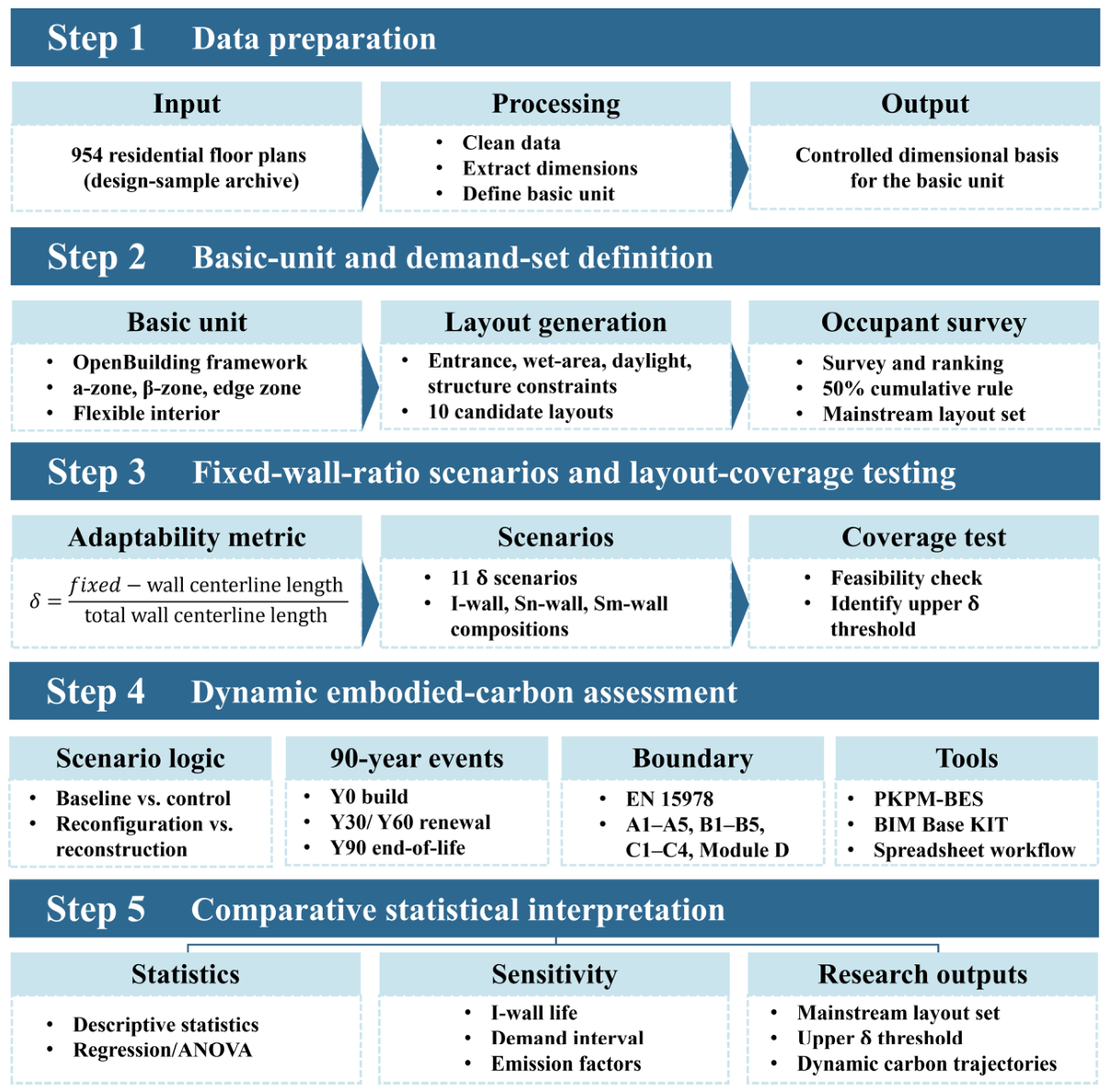
The research was organized into five stages: data preparation; basic-unit and demand-set definition; fixed-wall-ratio scenario construction and layout-coverage testing; dynamic embodied-carbon assessment; and comparative statistical interpretation. Figure 1 summarizes the datasets, analytical operations, calculation tools, and outputs, while the following subsections provide the procedures required to reproduce each stage.

The 90-year period is a potential-based analytical scenario rather than a description of the current average service life of Chinese housing. It was selected for two linked reasons. First, it contains three complete 30-year infill service cycles and therefore permits two intermediate renewal or reconstruction nodes at Years 30 and 60 before final end-of-life, making repeated update pathways directly comparable. Second, it approximates the long-life planning horizon associated with “century housing,” allowing the environmental consequences of retaining a long-lived support system while renewing shorter-lived infill components to be examined. This setting is particularly relevant because many Chinese residential buildings are reported to face major renovation or demolition after approximately 30–35 years of use—well before the nominal 50-year design life [23,65,66,67,68,69]. The 90-year horizon should therefore be understood as a forward-looking test of long-life potential and transferable design lessons, not as a forecast of present average practice. Alternative horizons and event frequencies are examined in Section 4.3.

2.1. Basic Unit Model

2.1.1. Development of the Basic Unit

(1)

Collection of residential layout data.

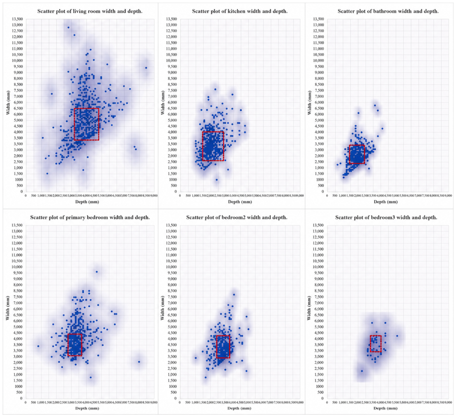
This study developed a common residential unit prototype, hereafter referred to as the “basic unit,” using a purposive design-sample archive assembled by the research team under a National Natural Science Foundation project [70]. The archive contained 954 contemporary residential floor plans. A plan was retained when its scale or dimension annotations, room functions, and principal spatial boundaries were sufficiently legible for measurement; duplicate and incomplete drawings were excluded during data cleaning. Living-room, bedroom, kitchen, and bathroom widths and depths were extracted from the available scale or dimension annotations and recorded in a structured dataset.

The extracted dimensions were summarized using scatter-density distributions. Concentrated width–depth ranges were then used to define the dimensional envelope of the controlled basic-unit prototype. The resulting distributions and adopted ranges are reported in Section 3.1, while the implications of the purposive sample for external validity are discussed in Section 4.5.

(2)

Development of the basic unit.

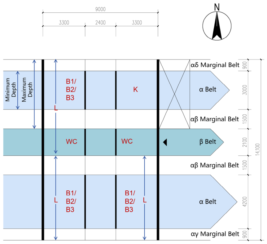
Within the theoretical framework of Open Building (OB), and under fixed constraints such as the structural system and service shaft locations, this study developed a residential “basic unit” with a flexible and transformable interior. To facilitate layout recombination and future updating, the basic unit was spatially zoned according to the logic of “fixed constraints versus flexible change” (Figure 2). The zone adjacent to the external façade and constrained by window placement and daylighting requirements was defined as the α-zone. The zone located in the interior of the plan and away from the external wall was defined as the β-zone. The intermediate flexible zone, which can be reallocated according to the needs of adjacent functional spaces, was defined as the edge zone. This zoning strategy established a clear spatial hierarchy: positions directly associated with the façade and structural boundary remain relatively stable, whereas the interior space retains higher flexibility. Based on this logic, a common residential “basic unit” with internal transformability was defined and used as the common plan prototype for generating the reconfigurable layout set, testing occupant-preference coverage, and constructing adaptability scenarios.

(3)

Generation of the reconfigurable layout set.

In theory, the flexible basic unit could generate many layout configurations. In actual residential design, however, multiple constraints substantially reduce the number of feasible schemes. The key constraints considered in this study include the following.

• Entrance and vertical circulation core constraint. The entrance door location is limited by the stairwell, elevator shaft, and corridor organization, thereby constraining the arrangement of the foyer and adjacent spaces.
• Wet-area alignment constraint. Kitchens and bathrooms must connect to fixed vertical service shafts and can therefore only be located in areas that satisfy plumbing and exhaust requirements.
• Bedroom daylighting constraint. At least one bedroom must be placed on the south side or the primary daylight façade to satisfy basic natural lighting requirements.
• Structural constraint. Major load-bearing structural positions remain fixed, some partitions must be coordinated with the structural grid, and large-span spaces must satisfy corresponding structural support requirements.

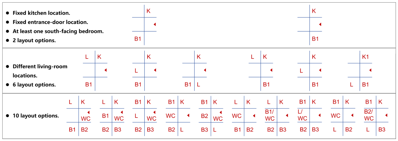
Under these constraints, a staged branching procedure was implemented (Figure 3). Starting from the fixed entrance, service-shaft, wet-area, and south-facing-bedroom requirements, alternative living-room positions and subsequent bedroom and bathroom subdivisions were enumerated. At each stage, branches that violated entrance access, wet-area connectivity, bedroom daylighting, or structural compatibility were removed. The retained layouts were then used as the candidate set for the household survey and subsequent layout-coverage testing; the retained branch counts are reported in Section 3.1.

2.1.2. Occupant Survey for the Basic Unit

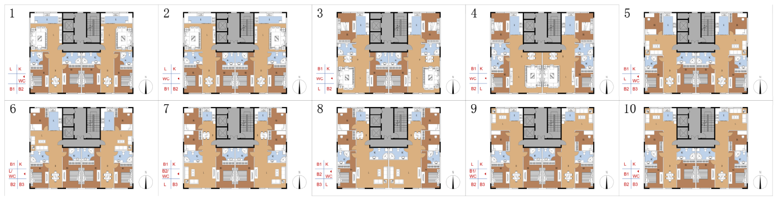
To identify the layouts with the highest occupant preference among the ten alternatives in the reconfigurable layout set and thereby further determine the mainstream layout set, a questionnaire survey was conducted (questionnaire provided in Supplementary Files). Figure 4 shows the ten layout plans used in the questionnaire. To ensure comparability among the alternatives, all plans used the same drawing scale, orientation, and standardized furniture arrangement. The first page of the questionnaire provided uniform instructions and examples, together with essential comprehension checks and basic demographic items. Data collection followed the principles of anonymity and informed consent and did not involve sensitive personal information. Overall preference was presented as selection frequency. To improve data quality, the questionnaire included basic logic checks and minimum response-time thresholds, and clearly invalid questionnaires were removed. All analyses were conducted on the cleaned valid dataset.

The core objective of the survey was to identify preferences for different spatial-organization schemes. Respondents could select more than one preferred layout. Accordingly, two denominators were reported separately: the respondent-level selection rate (frequency/168) and the share of all selections (frequency/313). To identify the mainstream layout set, layouts were ranked by frequency, and the smallest ranked set whose cumulative share of all selections first exceeded 50% was retained. This cumulative-selection rule provides an explicit cutoff for multiple-response data and avoids interpreting the share of all choices as the percentage of participants. The resulting mainstream layout set was then used as the reference for testing whether each δ scenario could continue to satisfy residential demand through internal reconfiguration.

Before formal distribution, five experts in architectural design and residential-behavior research evaluated the questionnaire in terms of relevance, clarity, completeness, length, and applicability using a 10-point scale. For the content validity index (CVI), scores of 8 or above were coded as relevant; item-level CVI (I-CVI) and the scale-level average CVI (S-CVI/Ave) were then calculated.

Questionnaire quality was further evaluated using the Kaiser–Meyer–Olkin (KMO) measure and Bartlett’s test of sphericity for factorability, Cronbach’s α for internal consistency, and a test–retest Spearman correlation for temporal stability. Repeated responses were obtained from a prespecified subset of the valid sample. The resulting validity and reliability statistics are reported in Section 3.1.

Survey responses were retained only after the logic and minimum-response-time checks described above. The cleaned dataset was then used to rank layout preferences and define the mainstream layout set.

2.1.3. Adaptive Component System for the Basic Unit

Based on the basic unit plan prototype, this study introduced a circular-component strategy using reversible connections so that spatial changes could be implemented through non-destructive disassembly and reassembly. The overall technical approach follows the support–infill separation principle: the support system satisfies long-term structural load-bearing and durability requirements, whereas the infill system provides adjustable spatial subdivision and allows disassembly, recovery, and recombination during use.

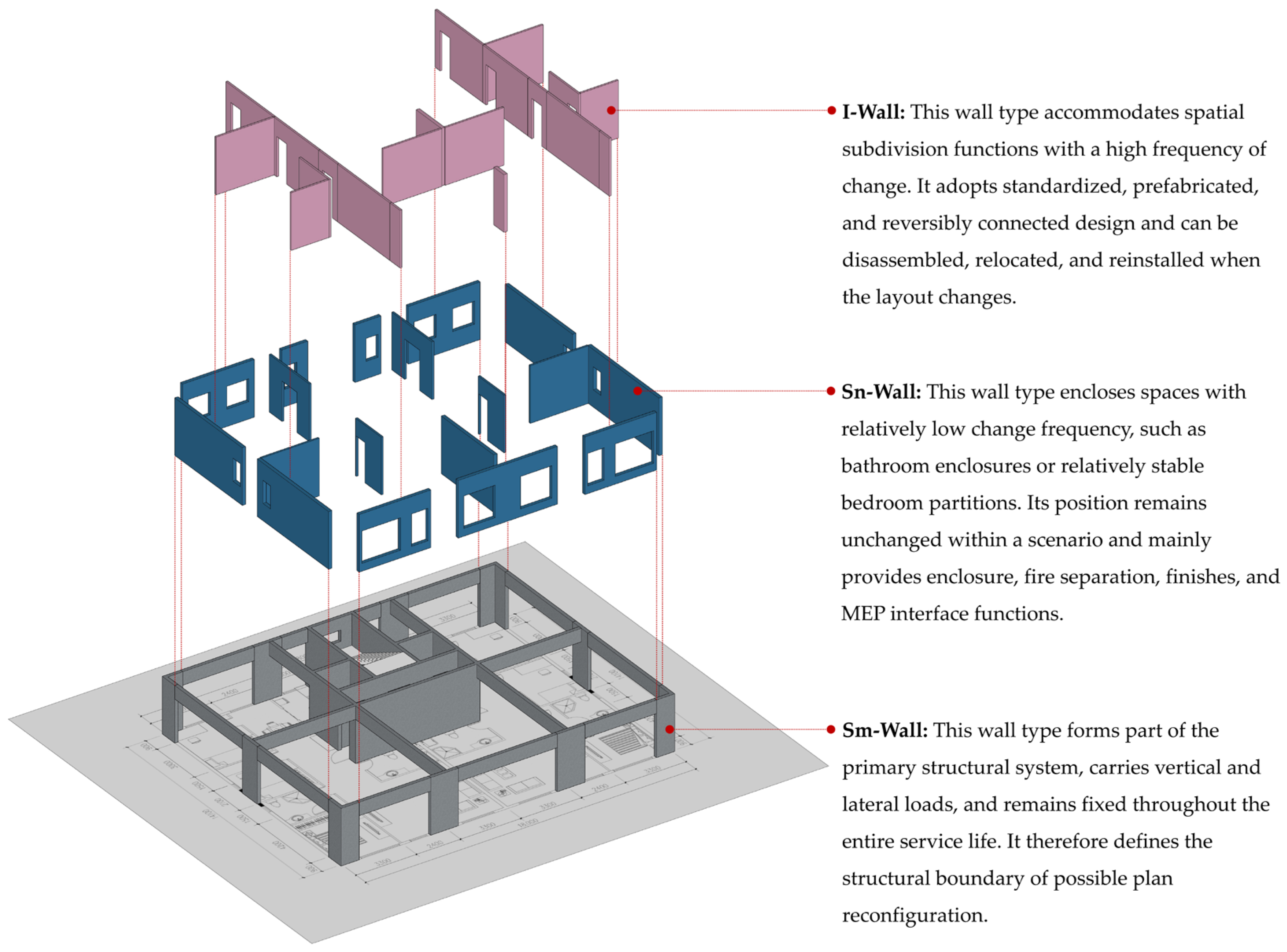
Accordingly, the wall components in the basic unit were divided into three categories (Figure 5).

• I-wall (movable non-load-bearing wall). This wall type accommodates spatial subdivision functions with a high frequency of change. It adopts standardized, prefabricated, and reversibly connected design and can be disassembled, relocated, and reinstalled when the layout changes.
• Sn-wall (fixed non-load-bearing wall). This wall type encloses spaces with relatively low change frequency, such as bathroom enclosures or relatively stable bedroom partitions. Its position remains unchanged within a scenario and mainly provides enclosure, fire separation, finishes, and MEP interface functions.
• Sm-wall (fixed load-bearing wall). This wall type forms part of the primary structural system, carries vertical and lateral loads, and remains fixed throughout the entire service life. It therefore defines the structural boundary of possible plan reconfiguration.

The circular components in this study use reversible connections and can therefore be repeatedly disassembled and reconfigured without damaging the components themselves. For example, an I-wall originally used to divide two rooms can be completely removed and relocated for reinstallation in a new position, or temporarily stored for future reuse, without destructive demolition. This classification provides a clear system boundary for the subsequent calculation of adaptability indicators, the specification of component renewal rules, and the embodied-carbon assessment over the residential life cycle.

2.2. Adaptability Metrics and Scenario Design

2.2.1. Adaptability Metric

This study used the basic unit as the analytical object and represented spatial constraint through the changeability of interior walls. To enable computable comparison, δ was defined as the proportion of fixed-wall centerline length within the interior-wall system. Thus, δ is not adaptability itself; it is an inverse proxy for adaptability and a direct indicator of fixedness. A lower δ means a larger share of movable I-walls and greater potential for layout transformation, whereas a higher δ means a larger share of fixed Sn-walls and Sm-walls and stronger spatial constraint.

The δ value was calculated using a consistent metric:

$$\mathsf{\delta }={\displaystyle \frac{L_{Sn}+L_{Sm}}{L_I+L_{Sn}+L_{Sm}}}$$

where L_I, L_Sn, and L_Sm denote the total centerline lengths of I-walls, Sn-walls, and Sm-walls, respectively. The accounting boundary was limited to the interior partition wall system of the residential unit and excluded external walls, curtain walls, and other envelope components in order to avoid interference from differences in the outer boundary condition. Door openings and service penetrations were measured continuously along the wall centerline and were not deducted, so as to reflect the actual level of spatial subdivision and transformation constraint. For example, when fixed walls and movable walls each account for 50% of the total wall centerline length, δ = 0.50.

In summary, δ should be interpreted as a fixed-wall-ratio indicator. As δ approaches 0, I-walls dominate and spatial adaptability increases; as δ approaches 1, fixed walls dominate and adaptability decreases. In the subsequent analysis, δ is treated as the principal control variable while structural form, unit boundary, time horizon, and accounting rules are held constant. The threshold reported below is therefore the upper δ value compatible with sufficient layout coverage, rather than a “minimum adaptability value.”

2.2.2. Scenario Design and Grouping

(1)

Adaptability scenarios.

Based on the basic-unit prototype, eleven δ scenarios were established: 0.32, 0.36, 0.42, 0.52, 0.59, 0.65, 0.72, 0.81, 0.88, 0.93, and 1.00; these represent a continuum from low fixedness/high adaptability to high fixedness/low adaptability. The number and positions of Sm-walls remained unchanged, and the total Sm-wall centerline length was fixed at 35.2 m because all schemes used the same structural system. Differences among scenarios were generated by varying the relative configuration of I-walls and Sn-walls.

The controlled substitution varied the relative configuration of I-walls and Sn-walls while holding the structural system, Sm-wall arrangement, unit boundary, time horizon, and accounting rules constant. All alternatives were assumed to satisfy minimum regulatory and functional requirements. Performance dimensions not included in the quantitative optimization are discussed separately in Section 4.5.

(2)

Service-life assumptions.

A common 90-year potential service-life scenario was adopted to capture repeated spatial adjustment and component renewal. Occupant spatial demand was assumed to change every 10 years, creating opportunities for layout adjustment before the final end-of-life year. The design service life of I-walls was assumed to be 30 years, leading to renewal events in Years 30 and 60. Sn-walls and Sm-walls were assumed not to require replacement under normal use during the 90-year period (

Table 1. Scenario settings and parameter comparison for the three wall types over a 90-year service life.

Item	I-Wall	Sn-Wall	Sm-Wall
Connection type	Reversible connection	Monolithic cast-in-place	Monolithic cast-in-place
Load-bearing status	Non-load-bearing	Non-load-bearing	Load-bearing
Service life	30 years	≥90 years	≥90 years
Adaptability	High (locally replaceable to accommodate change)	Low (functional change often requires full demolition)	Low (functional change often requires full demolition)
Demolition/renewal mode	Non-destructive disassembly; component recovery and reuse	Destructive demolition; converted into construction waste	Destructive demolition; converted into construction waste
Key events over 90 years	Layout changes every 10 years; renewal every 30 years	Overall demolition/recovery in Year 90	Overall demolition/recovery in Year 90

). These assumptions form a controlled base case; alternative horizons, demand-change intervals, and I-wall service lives are examined through an event-structure sensitivity check in Section 4.3.

(3)

System boundary.

The accounting boundary was defined at the level of one standard-story basic residential unit rather than the whole building. This was because multi-unit residential buildings usually show a high degree of repetition at the standard-floor level. Once the standard-floor plan composition and component configuration of the basic unit are defined, detailed assessment at this level can represent the embodied-carbon characteristics of similar repeated floors and can be scaled up to the whole building when necessary. Accordingly, the standard story with a floor height of 3 m was used as the accounting boundary, and the results can be expanded according to the actual number of floors or equivalent units.

The rectangular basic-unit boundary measures 9.0 m × 14.1 m, giving a gross floor area of A = 126.90 m². To support comparison with other studies and projects, each cumulative total E (tCO₂e) was additionally reported as an area-normalized intensity, I = 1000E/A (kgCO₂e/m²), for the same 90-year assessment period. Because all scenarios use the identical floor area, normalization does not change their relative ranking; it provides an additional reporting basis for cross-study comparison.

(4)

Scenario groups.

Based on the above settings, two comparison groups were further defined in order to compare the 90-year cumulative embodied carbon emissions of residential schemes with and without adaptability intervention.

• Baseline group. This group represents a dynamic scenario that considers changing occupant demand. If a residential unit can no longer satisfy mainstream occupant preferences through internal adjustment during the 90-year service life, the entire unit is demolished and reconstructed using a scheme capable of satisfying mainstream layout demand. If the unit can still satisfy mainstream demand, only the necessary internal reconfiguration is carried out. This group simulates the premature functional obsolescence of housing caused by insufficient adaptability.
• Control group. This group represents a static scenario that does not consider changing occupant demand. The residential unit is not adjusted during the 90-year service life regardless of the degree of match between the internal space and occupant demand. Taking component service life into account, the control group includes I-wall renewal in Year 30 and Year 60, while Sn-walls and Sm-walls remain unchanged over the entire period.

For the dynamic baseline group, the event algorithm was applied at each 10-year demand node. If the required mainstream layout was feasible, only the affected I-walls were reconfigured; if it was infeasible, demolition–reconstruction was triggered for the basic unit. At Years 30 and 60, scheduled I-wall renewal was counted only when the unit remained on the internal-reconfiguration pathway. When demolition–reconstruction occurred at the same node, reconstruction superseded the scheduled renewal event, thereby preventing double counting.

Through comparison between the baseline group and the control group, the study identifies the differences in 90-year cumulative embodied carbon emissions attributable to spatial adaptability intervention under consistent structural boundaries, service-life assumptions, and accounting rules, thereby evaluating the long-term carbon reduction effect of residential spatial adaptability.

2.3. Life-Cycle Embodied-Carbon Assessment Framework

2.3.1. Life-Cycle Embodied-Carbon Calculation

This study used EN 15978:2011 to calculate cumulative embodied carbon emissions over 90 years for each scenario. The assessment boundary covered the product stage (A1–A3), construction stage (A4–A5), use stage (B1–B5, excluding B6 and B7), end-of-life stage (C1–C4), and Module D beyond the life cycle, which accounts for emission reduction benefits from material recovery and reuse [70,71,72,73,74]. Because this study focuses on embodied carbon, operational carbon during building use, such as HVAC energy consumption, was excluded. However, maintenance and replacement activities associated with components during the use stage were included in the embodied-carbon calculation for stage B. Carbon emissions were calculated using the internationally established emission-factor method and in accordance with EN 15978. Material emission factors were taken mainly from the Chinese national standard, the Standard for Building Carbon Emission Calculation (GB/T 51366–2019), and the carbon emission parameters for construction and transportation were also taken from the recommended values of the same standard, ensuring reliability and consistency in the data source.

For each scenario, cumulative embodied carbon was calculated event by event as the sum of component quantity multiplied by the corresponding emission factor across A1–A5, B1–B5, and C1–C4, with Module D recovery and reuse benefits entered as negative credits. Initial construction was recorded at Year 0. Internal reconfiguration included only the I-wall quantities affected by each layout change; scheduled renewal replaced I-walls at their service-life nodes; and demolition–reconstruction included removal, waste transport and treatment, new material production, transport, construction, and the applicable recovery credits. This event structure was applied consistently to all δ scenarios.

2.3.2. Tools

This study used PKPM-BES (v2024), BIM Base KIT 2024, and an event-based spreadsheet workflow. BIM Base KIT was used to model wall components and transfer material and geometric information; PKPM-BES was used for quantity-based life-cycle calculations with emission factors aligned with GB/T 51366–2019; and spreadsheet equations represented component renewal, recovery, reuse, and reconstruction events that are not directly supported by the software. The study was conducted entirely in a digital modeling and calculation environment and did not involve physical laboratory equipment.

The hybrid model was evaluated primarily through internal consistency checks. Wall centerline lengths used in the δ calculation were reconciled with the geometric quantities transferred from the BIM model, and scenario totals were re-summed from exported quantities, emission factors, and event-based equations. This procedure checks arithmetic consistency and traceability across the BIM, PKPM, and spreadsheet layers. It does not constitute independent external validation against a third-party manual takeoff or long-term field observations. Accordingly, the results are interpreted as comparative scenario estimates under a common calculation framework rather than as universally validated absolute predictions.

The Supplementary Information provides the principal calculation inputs, wall quantities, emission-factor sources, component service-life assumptions, event equations, and analysis worksheets used to reproduce the scenario calculations. Recovery and reuse parameters follow the stated scenario assumptions rather than measured long-term recovery data; this evidence boundary is discussed in Section 4.5.

2.3.3. Statistical and Scenario Analysis

Descriptive statistics were used to summarize room dimensions, household composition, and layout-selection frequencies. Because the preference question allowed multiple responses, two denominators were reported separately: respondent-level selection rate (frequency/valid respondents) and share of all selections (frequency/total selections). Layouts were ranked by frequency, and the smallest ranked set whose cumulative share of all selections first exceeded 50% was defined as the mainstream layout set. For each δ scenario, every candidate layout was overlaid on the fixed Sn-wall and Sm-wall configuration and coded as feasible only when it could be realized by relocating, adding, or removing I-walls without moving fixed walls, while maintaining entrance access, service-shaft connectivity, wet-area alignment, bedroom daylighting, and structural compatibility. The upper fixed-wall-ratio threshold was defined as the largest tested δ value for which all layouts in the mainstream set received a feasibility code of 1.

For embodied-carbon analysis, a linear regression quantified the relationship between δ and 90-year cumulative emissions in the static control group. The dynamic baseline scenarios were divided at the coverage threshold and compared using one-way analysis of variance; η² was calculated as the effect-size measure, with p < 0.05 used as the significance criterion. A one-at-a-time event-structure sensitivity check compared alternative service-life horizons, I-wall service lives, and demand-change intervals. Descriptive statistics, regression, ANOVA, and event-count checks were implemented in the analysis workbook supplied with the Supplementary Information.

To examine sensitivity to regional or national carbon-data choices, a deterministic emission-factor screening was added. Multipliers of 0.80, 1.00, and 1.20 were applied coherently to all A1–C4 emission-factor terms and to the absolute magnitude of Module D credits, while component quantities, event timing, system boundaries, and layout-feasibility results were held constant. The ±20% interval is a transparent screening envelope rather than a statistical confidence interval or a direct substitution of a specific foreign database. In addition to coherent scaling, an adversarial adjacent-threshold comparison was made between δ = 0.72 under the +20% factor case and δ = 0.81 under the −20% factor case. This test evaluates whether the principal pathway contrast remains visible even when the sufficient-adaptability scenario is assigned higher coefficients and the insufficient-adaptability scenario lower coefficients.

3. Results

3.1. Basic-Unit Derivation and Questionnaire Evaluation Results

The 954-plan design sample produced concentrated but non-uniform width–depth distributions for the principal residential functions. Figure 6 presents the scatter-density patterns for living rooms, kitchens, bedrooms, primary bedrooms, studies, and bathrooms. The red dashed envelopes identify the dimensional ranges selected for basic-unit construction; these ranges provide a controlled design basis rather than estimates of the national prevalence of particular room sizes.

The constraint-based branching procedure retained two feasible spatial skeletons after applying the fixed entrance, shaft, and south-facing-bedroom requirements. Alternative living-room positions expanded these to six branches, and subsequent bedroom and bathroom subdivision produced ten feasible layouts (Figure 2). These ten layouts constituted the representative candidate set used in the occupant-preference survey and coverage analysis.

Expert evaluation indicated strong content validity. Mean scores for relevance, clarity, completeness, length, and applicability ranged from 8.4 to 8.7. With scores of 8 or above coded as relevant, all items achieved an I-CVI of 1.00 and the S-CVI/Ave was 1.00, exceeding the commonly recommended value of 0.90 (

Table 2. Expert review of questionnaire content validity.

Expert	Relevance (1–10)	Clarity (1–10)	Completeness (1–10)	Length (1–10)	Applicability (1–10)	Mean Score
E1	9	8.5	8.5	9	8.5	8.7
E2	8.5	8	9	8.5	8	8.4
E3	8.5	8.5	8.5	9	8.5	8.6
E4	8	8.5	8.5	8.5	9	8.5
E5	8.5	8.5	9	8.5	8.5	8.6
Mean	8.5	8.4	8.7	8.7	8.5	8.56

).

The KMO value was 0.82 and Bartlett’s test was significant (χ² = 320.7, df = 105, p < 0.001), supporting factorability. Cronbach’s α was 0.86 for the overall scale and 0.84 for the preference block, indicating good internal consistency. The test–retest Spearman correlation was ρ = 0.83 (p < 0.001), indicating strong temporal stability (

Table 3. Summary of questionnaire reliability and validity indices.

Index	Value	Interpretation
Cronbach’s α (overall scale)	0.86	Values > 0.8 indicate good internal consistency
Cronbach’s α (preference block)	0.84
KMO sampling adequacy	0.82	Values > 0.8 indicate good sampling adequacy
Bartlett’s test of sphericity	χ2 = 320.7, df = 105, p < 0.001	A significant result supports factorability
Test–retest correlation (Spearman ρ)	ρ = 0.83, p < 0.001	A strong significant correlation indicates temporal stability

).

Together, the dimensional analysis, transparent branching sequence, and questionnaire-quality results provide an auditable basis for the subsequent preference ranking, coverage testing, and dynamic embodied-carbon comparison.

3.2. Questionnaire Preferences and Mainstream Layout Set

The questionnaire survey was conducted from October 2024 to January 2025 and yielded 168 valid responses. The sample was dominated by three- and four-person households: three-person households accounted for 35.1% (n = 59) and four-person households for 41.1% (n = 69), representing 76.2% of the total sample combined; two-person households and households with five or more persons each accounted for 11.9% (n = 20). This sample structure indicates that the questionnaire mainly reflects the dominant preferences of typical three- to four-person households regarding housing layout organization and adaptability. In addition, 60% of the sample (n = 100) completed repeated measurements, providing the basis for questionnaire reliability testing (

Table 4. Sample characteristics and household composition.

Household Size	n	%
1 person	—	—
2 persons	20	11.9
3 persons	59	35.1
4 persons	69	41.1
≥5 persons	20	11.9
Total sample size	168	100
Retest sample	100	60

).

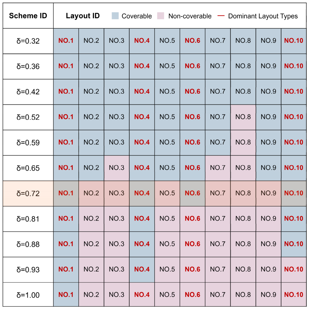
The multiple-response question produced 313 selections, equivalent to an average of 1.86 selections per respondent. Layouts were ranked by frequency to apply the cumulative 50% rule. Layout 1 contributed 17.6% of all selections, followed by Layout 6 (14.1%), Layout 4 (13.7%), and Layout 10 (12.8%). The first three layouts together accounted for 45.4% of all selections; adding Layout 10 increased the cumulative share to 58.1%. Therefore, Layouts 1, 6, 4, and 10 constitute the smallest ranked set whose cumulative share exceeds 50% and were defined as the mainstream layout set. The value 58.1% refers to the share of all selections (182/313), not to the share of participants. Layouts 3 and 5 each had a respondent-level selection rate of 18.5%, but each contributed only 9.9% of all selections and was not required once the cumulative threshold had been crossed (

Table 5. Frequency distribution of preferences across the ten candidate layouts.

Layout ID	Frequency	Respondent Selection Rate (%)	Share of all Selections (%)
Layout 1	55	32.7	17.6
Layout 6	44	26.2	14.1
Layout 4	43	25.6	13.7
Layout 10	40	23.8	12.8
Layout 3	31	18.5	9.9
Layout 5	31	18.5	9.9
Layout 7	26	15.5	8.3
Layout 8	20	11.9	6.4
Layout 2	19	11.3	6.1
Layout 9	4	2.4	1.3

).

Building on the questionnaire results, the wall-based δ value was used to test layout coverage under each scenario (Figure 7). The number of coverable layouts decreases as δ increases. At δ = 0.32–0.42, all ten layouts are feasible; at δ = 0.52, 0.59, and 0.65, the number falls to 9, 8, and 7, respectively. At δ = 0.72, four layouts remain feasible, and they correspond exactly to the mainstream set identified by the cumulative-selection rule (Layouts 1, 6, 4, and 10). When δ increases to 0.81 or above, at least one mainstream layout becomes infeasible. Thus, δ ≈ 0.72 is the largest tested fixed-wall ratio that remains compatible with full mainstream-layout coverage. Equivalently, δ ≤ 0.72 indicates sufficient adaptability under the study conditions, whereas δ > 0.72 does not.

Accordingly, δ ≈ 0.72 was used in the dynamic carbon scenarios as the upper fixed-wall-ratio threshold for maintaining full coverage of the mainstream layout set. This terminology distinguishes the measured fixedness ratio from the underlying concept of adaptability.

3.3. Embodied-Carbon Comparison Across δ-Value Scenarios

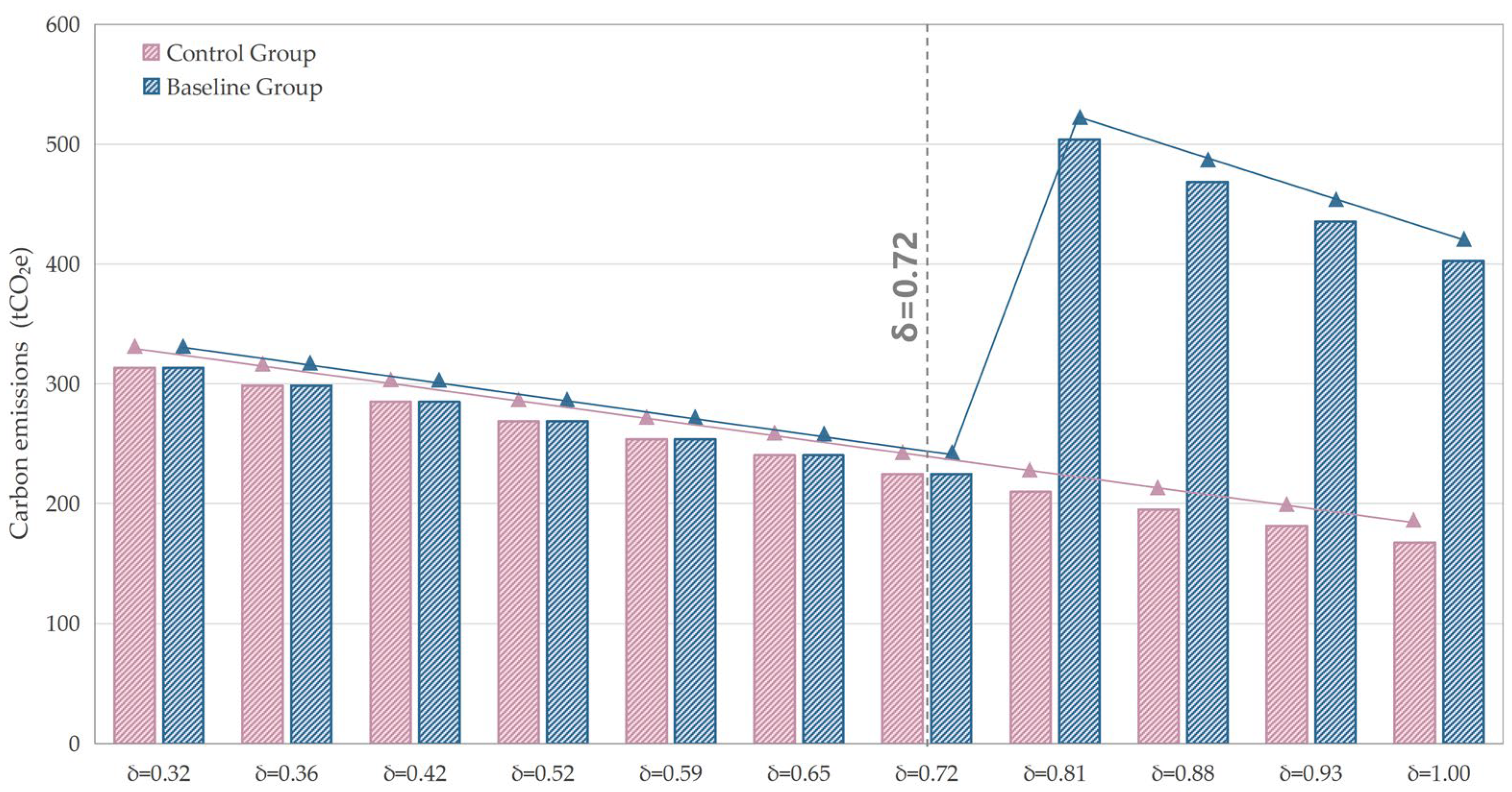
This study compared the 90-year cumulative embodied carbon emissions of the eleven δ-value scenarios in both the baseline group and the control group. The results show that in the control group, cumulative embodied carbon emissions decrease significantly and almost linearly as δ increases from 0.32 to 1.00 (Figure 8). Specifically, the δ = 0.32 scheme yields 313.46 tCO₂e (2470.13 kgCO₂e/m²) over 90 years, whereas the δ = 1.00 scheme yields 167.76 tCO₂e (1321.99 kgCO₂e/m²). Linear regression shows an extremely significant negative correlation between δ and 90-year cumulative embodied carbon in the control group: for every 0.1 increase in δ, emissions decrease by approximately 20.72 tCO₂e, or 163.28 kgCO₂e/m², on average (R² ≈ 0.998, p ≈ 2.55 × 10⁻¹³ < 0.001). This indicates that improving spatial adaptability requires more movable partitions and their associated renewal processes, thereby increasing embodied carbon from initial construction and periodic renewal.

In the baseline group, which represents dynamic updating, carbon outcomes show a nonlinear jump. When δ ≤ 0.72, all mainstream layouts remain achievable through internal reconfiguration, and cumulative emissions range from 224.88 to 313.46 tCO₂e (1772.10–2470.13 kgCO₂e/m²). When δ > 0.72, at least one mainstream layout becomes infeasible and demolition–reconstruction is triggered at the modeled update nodes, increasing totals to 402.62–503.95 tCO₂e (3172.73–3971.24 kgCO₂e/m²). The largest tested δ compatible with full coverage, δ = 0.72, completes the 90-year scenario without reconstruction and emits 224.88 tCO₂e (1772.10 kgCO₂e/m²). By contrast, δ = 0.81 triggers two demolition–reconstruction events and reaches 503.95 tCO₂e (3971.24 kgCO₂e/m²).

To clarify the temporal mechanism behind this jump, Figure 9 compares the dynamic evolution of cumulative embodied carbon for the representative δ = 0.72 and δ = 0.81 scenarios at 10-year intervals. Before the first major update node, the δ = 0.81 scheme has slightly lower cumulative emissions because it contains fewer movable I-walls. At Years 30 and 60, however, the two pathways diverge: the δ = 0.72 scheme remains capable of satisfying mainstream layout demand through internal reconfiguration and records only limited increments associated with scheduled I-wall renewal, whereas the δ = 0.81 scheme undergoes demolition–reconstruction and exhibits two pronounced emission jumps. By Year 90, cumulative emissions reach 224.88 tCO₂e (1772.10 kgCO₂e/m²) for δ = 0.72 and 503.95 tCO₂e (3971.24 kgCO₂e/m²) for δ = 0.81. The dynamic trajectories therefore show that the discontinuity is produced by a change in update pathway rather than by the fixed-wall ratio alone.

Table 6. Comparison of 90-year cumulative embodied carbon totals and area-normalized intensities under different δ-value scenarios. Values in parentheses are kgCO₂e/m² based on A = 126.90 m².

Scenarios	Baseline Group (tCO2e; kgCO2e/m2)		Control Group (tCO2e; kgCO2e/m2)
δ = 0.32	313.46 tCO2e	2470.13 kgCO2e/m2	313.46 tCO2e	2470.13 kgCO2e/m2
δ = 0.36	298.65 tCO2e	2353.43 kgCO2e/m2	298.65 tCO2e	2353.43 kgCO2e/m2
δ = 0.42	285.00 tCO2e	2245.86 kgCO2e/m2	285.00 tCO2e	2245.86 kgCO2e/m2
δ = 0.52	268.94 tCO2e	2119.31 kgCO2e/m2	268.94 tCO2e	2119.31 kgCO2e/m2
δ = 0.59	254.06 tCO2e	2002.05 kgCO2e/m2	254.06 tCO2e	2002.05 kgCO2e/m2
δ = 0.65	240.40 tCO2e	1894.41 kgCO2e/m2	240.40 tCO2e	1894.41 kgCO2e/m2
δ = 0.72	224.88 tCO2e	1772.10 kgCO2e/m2	224.88 tCO2e	1772.10 kgCO2e/m2
δ = 0.81	503.95 tCO2e	3971.24 kgCO2e/m2	209.98 tCO2e	1654.69 kgCO2e/m2
δ = 0.88	468.41 tCO2e	3691.17 kgCO2e/m2	195.17 tCO2e	1537.98 kgCO2e/m2
δ = 0.93	435.65 tCO2e	3433.02 kgCO2e/m2	181.52 tCO2e	1430.42 kgCO2e/m2
δ = 1.00	402.62 tCO2e	3172.73 kgCO2e/m2	167.76 tCO2e	1321.99 kgCO2e/m2

summarizes all eleven scenarios. Two mechanisms operate simultaneously: increasing adaptability requires more movable components and raises initial and renewal-related emissions, whereas insufficient adaptability can trigger demolition–reconstruction during long-term use. Figure 9 clarifies their temporal relationship. The δ = 0.81 scheme begins with a modest carbon advantage over δ = 0.72, but this advantage disappears at the first demolition–reconstruction event in Year 30; a second event in Year 60 further widens the cumulative-emission gap. Thus, once the upper δ threshold is exceeded, the long-term carbon burden of pathway change dominates the initial savings associated with fewer movable components.

Overall, the objective is not to maximize adaptability without limit. The carbon-relevant design condition is to keep δ at or below the upper threshold required for mainstream-layout coverage. Under the present basic-unit and demand assumptions, δ ≈ 0.72 is the largest tested fixed-wall ratio that avoids the modeled transition to demolition–reconstruction.

3.4. Coupling Mechanism Between Spatial Adaptability and Embodied Carbon

The relationship between residential adaptability and whole-life embodied carbon is not linear. Under static conditions, lower δ values require more movable partitions and increase routine embodied carbon. Under dynamic conditions, however, crossing the upper fixed-wall-ratio threshold changes the modeled update pathway: the unit can no longer cover the mainstream layout set internally and moves to demolition–reconstruction, causing a discontinuous increase in cumulative emissions. Static assessment alone may therefore underestimate the long-term carbon penalty associated with excessive spatial fixedness.

From both theoretical and practical perspectives, the findings indicate that although higher spatial adaptability increases upfront embodied carbon, this increase can be offset—and even transformed into a net carbon benefit—over the full service life by avoiding demolition–reconstruction. At the same time, this study responds to ongoing interest in dynamic life-cycle assessment in the building field. Most previous LCA studies have assumed static building configurations over the full life span and have rarely incorporated explicit occupant demand change and spatial updating processes [53,54,55,56,57,58,59,60]. By contrast, the dynamic scenario simulation in this study shows that the time dimension and spatial adaptability variable jointly reshape embodied-carbon outcomes in residential buildings.

In summary, the key result is not that “more adaptability is always better,” but that a maximum level of fixedness must not be exceeded if mainstream spatial demand is to remain coverable. The upper δ threshold provides an operational design control variable, while the associated carbon results quantify the consequences of crossing it.

4. Discussion

4.1. Threshold Effect and Mechanistic Interpretation

The results show that spatial adaptability changes the evolution pathway of whole-life embodied carbon. In the static control group, cumulative emissions decline almost linearly as δ increases because fewer movable partitions are installed and renewed. In the dynamic baseline group, the relationship becomes nonlinear: once δ exceeds the largest value compatible with mainstream-layout coverage, the update pathway changes from internal reconfiguration to demolition–reconstruction.

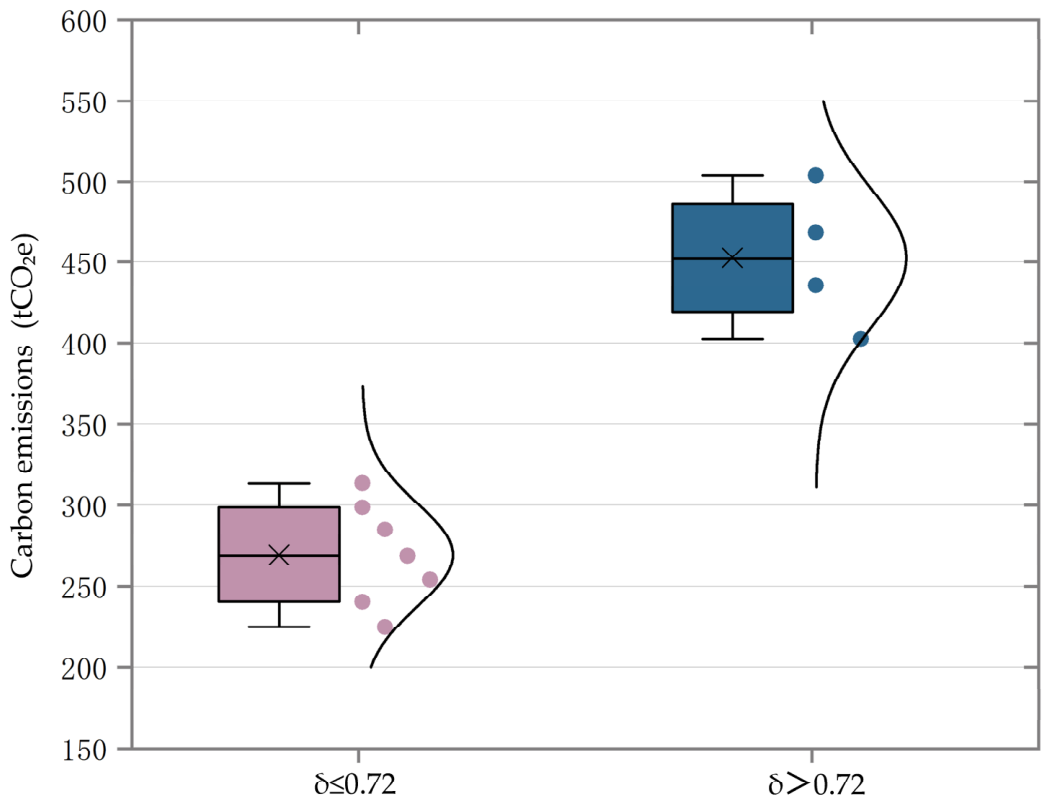
To verify the threshold effect of δ ≈ 0.72 statistically, the baseline-group samples were divided into two groups according to whether they crossed the threshold of δ = 0.72, and a box plot was used to show the dispersion characteristics of 90-year cumulative embodied carbon in the two groups (Figure 10). The results show complete separation between the two distributions. Before the threshold (δ ≤ 0.72, n = 7), embodied carbon emissions are concentrated in the range of approximately 225–313 tCO₂e, with a median of about 268.94 tCO₂e and an interquartile range of about 44.60 tCO₂e. After the threshold (δ > 0.72, n = 4), the distribution shifts upward to approximately 403–504 tCO₂e, with a median of about 452.03 tCO₂e and an interquartile range of about 49.90 tCO₂e. The absence of overlap between the boxes and whiskers indicates a structural jump in carbon emissions after the threshold is crossed. Further analysis of variance (ANOVA) shows that the difference in mean 90-year cumulative embodied carbon before and after δ = 0.72 is highly significant, with F(1,9) = 65.40 and p ≈ 2.03 × 10⁻⁵ < 0.01 (

Table 7. Analysis of variance (ANOVA).

Source	SS	df	MS	F	p
Between groups (before vs. after threshold: δ ≤ 0.72 vs. δ > 0.72)	85,539.4452	1	85,539.4452	65.4038	2.03 × 10−5
Within groups (error)	11,770.8080	9	1307.8676	—	—

). The threshold grouping also explains a large proportion of the total variance (η² ≈ 0.88). This indicates that once spatial adaptability is no longer sufficient to fully cover the mainstream layout set, the residential update pathway shifts from internal reconfiguration to demolition–reconstruction, triggering a significant increase in cumulative embodied carbon. Together, the box plot and ANOVA results confirm a strongly coupled nonlinear threshold relationship between spatial adaptability and embodied carbon under dynamic demand conditions.

Mechanistically, higher spatial adaptability (i.e., lower δ values) supports a high-frequency, low-intensity update mode. In this mode, layout adjustment is achieved primarily through the reconfiguration of existing I-walls, and embodied carbon changes relatively smoothly over time, with more concentrated emission events occurring only when I-walls reach the end of their service life and are renewed, such as in Year 30 and Year 60. By contrast, lower spatial adaptability (i.e., higher δ values) sharply restricts the ability of a residential unit to cover the mainstream layout set. Once occupant demand exceeds the unit’s internal adjustment capacity, the update pathway shifts to a low-frequency, high-intensity demolition–reconstruction mode. This creates significant carbon peaks in reconstruction years and leads to a stepwise increase in cumulative embodied carbon.

It is important to note that high adaptability is not cost-free. In the control group, for example, the δ = 0.32 scheme emits 313.46 tCO₂e over 90 years, about 86.9% higher than the δ = 1.00 scheme at 167.76 tCO₂e, confirming that higher adaptability increases component input and renewal-related emissions. In the baseline group, however, this upfront increment is far smaller than the long-term benefit of avoiding demolition–reconstruction: the δ = 0.72 scheme emits 224.88 tCO₂e over 90 years, which is 55.4% and 44.1% lower than the δ = 0.81 and δ = 1.00 schemes, respectively. This indicates that, from a whole-life perspective, the carbon advantage of maintaining sufficient adaptability to cover the mainstream layout set comes mainly from avoiding demolition–reconstruction rather than from reducing initial construction emissions.

In summary, maintaining δ at or below the upper fixed-wall-ratio threshold may increase routine component-related emissions relative to a rigid configuration, but it can substantially reduce reconstruction-related carbon peaks over the whole life cycle.

4.2. Role of Recyclable Components in Spatial Adaptability and Carbon Reduction

Spatial adaptability produces measurable carbon reductions largely through reusable prefabricated components. Through a support–infill separation strategy, residential buildings can adjust layouts by disassembling and repositioning prefabricated internal partitions and other infill components without making destructive changes to the main structural system. Under these conditions, functional reorganization depends primarily on repeated use and localized replacement of existing components rather than complete demolition and reconstruction, thereby reducing material consumption and embodied carbon during updating. At the component level, disassembly and circular reuse therefore convert spatial adaptability into quantifiable carbon benefits.

More importantly, the integration of spatial adaptability with circular components is consistent with the core principles of the circular economy in the building sector. Many scholars have argued that the multiple-use potential of building components should be considered in advance during design and then tracked across the life cycle in order to minimize material waste and embodied carbon and ultimately move toward near-zero-carbon construction [75,76,77,78,79,80]. This view is consistent with the findings of the present study. Reversible connections and circular reuse at the component level create favorable conditions for the high-frequency, low-intensity update pathway, thereby avoiding the carbon peaks associated with the low-frequency, high-intensity demolition–reconstruction pathway. Consequently, combining easily detachable and reusable component technologies with spatial adaptability design is an effective route toward carbon reduction in residential construction.

Recent research on nearly zero-energy buildings has continued to improve operational performance through semi-transparent photovoltaic double-skin façades and experimentally validated Trombe-wall systems [81,82,83]. These studies focus primarily on thermal behavior and operational-energy reduction rather than spatial adaptability or component-related embodied carbon. Their inclusion nevertheless clarifies the wider decarbonization context: as operational demand is reduced through advanced envelope and passive-energy technologies, the relative importance of avoiding repeated material input, premature reconstruction, and embodied-carbon peaks becomes increasingly significant.

4.3. Sensitivity and Robustness of Temporal and Emission-Factor Assumptions

A one-at-a-time event-structure sensitivity check was conducted for the principal temporal assumptions. For potential service-life horizons of 60, 90, and 120 years, the number of intermediate 30-year renewal or reconstruction nodes is one, two, and three, respectively. Over a 90-year horizon, I-wall service lives of 20, 30, and 40 years produce four, two, and two replacement events before final end-of-life, respectively. Demand-change intervals of 5, 10, and 15 years produce 17, 8, and 5 internal-reconfiguration opportunities before Year 90. These alternatives change the frequency and magnitude of B4 and reconstruction-related emissions, but they do not change the geometric coverage result that δ = 0.72 is the largest tested ratio at which all four mainstream layouts remain feasible.

The carbon advantage of sufficient adaptability is expected to increase with a longer horizon or a larger number of reconstruction nodes and to decrease under a shorter horizon. A 20-year I-wall life increases renewal events relative to the base case, whereas a 40-year life shifts renewal timing but does not reduce the number of pre-end-of-life replacements within 90 years. Partial Sn-wall replacement would increase totals in both groups and could alter the magnitude of the gap, although the threshold classification would remain unchanged unless replacement itself changed layout coverage. Because independent probability distributions and component-specific degradation data were not available, this check evaluates event-count sensitivity rather than providing a full probabilistic uncertainty analysis.

The emission-factor screening changes absolute carbon totals but not the geometric coverage threshold or the ordering of scenarios when the same multiplier is applied coherently. For δ = 0.72, the −20%, base, and +20% cases are 179.90, 224.88, and 269.86 tCO₂e, respectively (1417.68, 1772.10, and 2126.52 kgCO₂e/m²). For δ = 0.81, the corresponding values are 403.16, 503.95, and 604.74 tCO₂e (3176.99, 3971.24, and 4765.49 kgCO₂e/m²). In the deliberately adverse cross-case comparison, δ = 0.81 at −20% still exceeds δ = 0.72 at +20% by 133.30 tCO₂e, or 49.4%. Thus, the adjacent threshold-related shift from internal reconfiguration to demolition–reconstruction remains robust within this screening envelope (

Table 8. Deterministic emission-factor sensitivity of the representative δ = 0.72 and δ = 0.81 scenarios. Values in parentheses are kgCO₂e/m² based on A = 126.90m².

Scenario	−20% Factors (tCO2e; kgCO2e/m2)		Base Factors (tCO2e; kgCO2e/m2)		+20% Factors (tCO2e; kgCO2e/m2)
δ = 0.72	179.90	1417.68	224.88	1772.10	269.86	2126.52
δ = 0.81	403.16	3176.99	503.95	3971.24	604.74	4765.49

).

This result supports transfer of the mechanism, not direct transfer of the Chinese numerical totals. National databases may differ by material production technology, electricity mix, transport, waste treatment, data age, and module coverage; phase-specific substitutions may therefore change the magnitude of each scenario. A fully harmonized EU–China–India database comparison would require product-by-product mapping under identical functional units and EN 15978 boundaries and is identified as a priority for future work.

4.4. International Transferability and Translation into Design Standards and Rating Tools

The internationally transferable contribution of this study is the analytical protocol rather than the numerical value δ≈0.72 itself. For application in the European Union, the same wall-based and event-based workflow can be aligned with EN 15978 and Level(s) Indicator 1.2, while replacing the Chinese emission factors with applicable national databases, EPDs, transport scenarios, and end-of-life rules [61,62]. For India and other rapidly urbanizing markets, the workflow can be combined with locally representative material inventories and construction practices, consistent with Indian research emphasizing context-specific regional and temporal LCI data [63,64].

A cross-market application should therefore follow five steps: (1) reconstruct the local basic-unit and household-demand set; (2) apply local codes and climatic or cultural requirements to layout feasibility; (3) recalculate the upper δ threshold; (4) substitute local A1–D factors, transport distances, service lives, and recovery scenarios; and (5) report both total and area-normalized results with uncertainty or sensitivity ranges. Researchers can use this protocol to compare adaptability–carbon mechanisms across housing stocks; practitioners can use the coverage matrix and δ calculation for early scheme screening; and policy or rating-system developers can use the documented evidence chain to formulate locally calibrated credits or disclosure requirements.

The upper δ threshold can be translated into a project-specific compliance check rather than treated as a universal code value. At concept design, the project team should define the target layout-demand set, classify interior walls as I-wall, Sn-wall, or Sm-wall, calculate δ from the wall-centerline schedule, and test whether every target layout can be achieved without relocating fixed walls. Under the basic-unit and demand conditions examined here, δ ≤ 0.72 passes this screening test, whereas δ > 0.72 signals the need to reduce fixed-wall length or reposition fixed walls before the scheme is developed further.

For design standards or voluntary rating systems, the procedure can be organized as three evidence levels: (1) mandatory disclosure of the wall classification, δ value, and target layout set; (2) a performance credit for demonstrating full target-set coverage at or below the project-specific threshold; and (3) an enhanced credit for combining threshold compliance with reversible connections, a component-reuse plan, and quantified whole-life carbon savings. Verification can be repeated at concept design, technical design, and as-built stages using the same BIM-based wall schedule and coverage matrix. This structure is analogous to the staged evidence and outcome-benchmarking logic used in major green-building systems, but it does not imply that existing LEED or BREEAM schemes currently prescribe a δ threshold.

Before formal codification, the numerical threshold should be recalibrated for different unit geometries, household-demand sets, structural systems, and regional practices, and should be checked jointly with acoustic, fire-safety, accessibility, service, constructability, cost, and user-acceptance requirements. Accordingly, δ ≈ 0.72 is proposed here as an evidence-based screening and credit criterion for the tested residential prototype, not as a universally applicable regulatory limit.

4.5. Limitations and Future Work

Although this study provides a controlled quantitative account of the relationship between spatial constraint and embodied carbon, the proposed threshold and implementation pathway should be interpreted within the following boundaries.

First, δ is a fixed-wall-ratio proxy rather than a direct or universal measure of adaptability. The numerical threshold is conditional on the basic-unit geometry, wall classification, mainstream-layout definition, and coverage rule used here. Other housing types or demand sets may produce a different upper δ threshold.

Second, the 954-plan database is a purposive design sample rather than a probability sample of the Chinese housing stock, and complete geographical and temporal metadata were unavailable for every plan. Moreover, the branching procedure was exhaustive only within the predefined zoning framework, sequence of functional-space placement, and feasibility constraints; it did not enumerate every geometrically possible residential plan. Broader regional samples and generative plan-space enumeration are therefore required to test the external validity of the basic unit, candidate layout set, and upper δ threshold.

Third, varying I-wall and Sn-wall proportions may influence acoustics, fire performance, privacy, service access, constructability, cost, and user acceptance. These dimensions were treated as minimum design constraints rather than quantified objectives. The δ threshold should therefore be used as one carbon-related criterion within a multi-criteria design process, not as a stand-alone prescriptive optimum.

Fourth, the event-structure sensitivity check shows the direction of change under alternative service lives and update intervals, but a full recalculation with probabilistic degradation, partial Sn-wall replacement, and uncertain occupant behavior was beyond the available data. The 90-year results should therefore be interpreted as a potential-based scenario comparison rather than a forecast of current average practice.

Fifth, the BIM–PKPM–spreadsheet workflow was checked for internal consistency but was not independently validated against a third-party manual quantity takeoff or long-term empirical recovery data. Figure 9 clarifies the timing of pathway divergence and distinguishes scheduled I-wall renewal from demolition–reconstruction events, but it does not provide a complete component-level decomposition of initial construction, internal reconfiguration, component renewal, demolition–reconstruction, end-of-life treatment, and Module D credits. A finer event-by-event and life-cycle-module disaggregation should therefore be developed when more detailed calculation records become available.

Sixth, the emission-factor analysis uses a coherent ±20% deterministic perturbation and does not reproduce the phase-specific structure of any individual European, Indian, or other national database. It demonstrates the stability of the adjacent threshold-related pathway contrast under a transparent coefficient envelope, but it cannot establish numerical equivalence across markets. Direct international comparison requires harmonized product mapping, functional units, data quality periods, electricity and transport assumptions, waste scenarios, and Module D conventions.

Future research should combine broader regional plan datasets, automated plan-space enumeration, multi-performance evaluation, probabilistic service-life modeling, longitudinal observation of adaptable housing projects, and harmonized recalculation using European, Indian, and other national LCI or EPD datasets. These extensions would test both the transferability of the analytical method and the context dependence of the upper δ threshold, while strengthening the empirical basis for low-carbon residential design standards and circular-component strategies.

5. Conclusions

This study establishes an occupant-demand-linked framework for relating residential spatial fixedness to dynamic whole-life embodied carbon. By connecting layout-coverage requirements with a computable fixed-wall ratio and time-dependent updating pathways, it advances adaptability assessment from a qualitative design intention toward a testable carbon-control criterion.

(1)

Under the stated basic-unit and household-demand conditions, δ ≈ 0.72 is the largest tested fixed-wall ratio compatible with full coverage of the mainstream layout set. Values at or below this threshold retain sufficient internal-reconfiguration capacity, whereas higher values cause at least one mainstream layout to become infeasible.

(2)

The embodied-carbon effect is pathway-dependent rather than linear. Scenarios with δ ≤ 0.72 remain on an internal-reconfiguration pathway and produce 224.88–313.46 tCO₂e over 90 years (1772.10–2470.13 kgCO₂e/m²). When δ > 0.72, the modeled pathway shifts to demolition–reconstruction and cumulative emissions increase to 402.62–503.95 tCO₂e (3172.73–3971.24 kgCO₂e/m²); the representative trajectories show that reconstruction events at Years 30 and 60 dominate the initial savings from using fewer movable components.

The principal scientific contribution is the integration of occupant preference, spatial coverage, and dynamic life-cycle assessment within one controlled analytical framework. In practice, the upper δ threshold can be used as a project-specific early-design screening criterion supported by a wall-classification plan, wall-centerline schedule, layout-coverage matrix, and whole-life carbon assessment. It can also inform future voluntary credits for adaptable and circular residential design, provided that the threshold is recalibrated for other housing types and applied alongside acoustic, fire-safety, service-access, constructability, cost, accessibility, and user-acceptance requirements.

For international readers, the added value lies in a reproducible sequence of skills and decisions: deriving a locally relevant demand set, quantifying spatial fixedness, testing layout coverage, representing update events over time, substituting regional carbon data, and evaluating whether an apparently material-efficient rigid scheme creates higher long-term reconstruction emissions. The method can therefore support comparative research, early-stage professional design decisions, and the development of locally calibrated assessment criteria in both mature European markets and rapidly urbanizing contexts such as India. The numerical threshold and carbon totals should not be transferred without recalibration, but the mechanism-based workflow provides a common basis for such recalibration.

References

1. Legg, S. IPCC, 2021: Climate change 2021-the physical science basis. Interaction 2021, 49, 44–45. [Google Scholar]
2. Kumar, D.; Maurya, K.K.; Mandal, S.K.; Mir, B.A.; Nurdiawati, A.; Al-Ghamdi, S.G. Life cycle assessment in the early design phase of buildings: Strategies, tools, and future directions. Buildings 2025, 15, 1612. [Google Scholar] [CrossRef]
3. Chen, C.; Zhao, Z.; Xiao, J.; Tiong, R. A conceptual framework for estimating building embodied carbon based on digital twin technology and life cycle assessment. Sustainability 2021, 13, 13875. [Google Scholar] [CrossRef]
4. Bacheva, T.S.; Raposo Grau, J.F. Embodied imapacts in buildings: A systematic review of life cycle gaps and sectoral integration strategies. Buildings 2025, 15, 1661. [Google Scholar] [CrossRef]
5. Mir, B.A.; Nurdiawati, A.; Al-Ghamdi, S.G. Guiding Decarbonizing of the Built Environment: Trends, Methods, and Approaches for Carbon Benchmarking in Buildings. Buildings 2026, 16, 708. [Google Scholar] [CrossRef]
6. Sandaruwan, I.P.T.; Allis, C.; Siriwardena, M. Building Green, Consuming Embodied Energy? Cradle-to-Gate Embodied Energy Assessment of Green Office Buildings for a Sustainable Built Environment in Sri Lanka. Buildings 2025, 15, 2819. [Google Scholar] [CrossRef]
7. Fu, Y.; Wang, C.C. Optimisation of Embodied Carbon and Thermal Performance of Roof Material Selections for Australian Residential Housing. Buildings 2025, 15, 268. [Google Scholar] [CrossRef]
8. Huang, Y.; Wang, F.; Hiscock, A.V.; Satyarthi, J.; Smith, H. Including embodied carbon in assessing renovation options for industrial heritage buildings: A review and case studies. Sustainability 2025, 17, 72. [Google Scholar] [CrossRef]
9. Lützkendorf, T.; Balouktsi, M. Embodied carbon emissions in buildings: Explanations, interpretations, recommendations. Build. Cities 2022, 3, 964–973. [Google Scholar] [CrossRef]
10. Janjua, S.Y.; Sarker, P.K.; Biswas, W.K. Impact of service life on the environmental performance of buildings. Buildings 2019, 9, 9. [Google Scholar] [CrossRef]
11. Lim, H. Comparative Life Cycle Assessment of Reconstruction and Renovation for Carbon Reduction in Buildings. Buildings 2025, 15, 3388. [Google Scholar] [CrossRef]
12. Leichter, M.; Piccardo, C. Assessing life cycle sustainability of building renovation and reconstruction: A comprehensive review of case studies and methods. Build. Environ. 2024, 262, 111817. [Google Scholar] [CrossRef]
13. Di Bari, R.; Belleri, A.; Marini, A.; Horn, R.; Gantner, J. Probabilistic life-cycle assessment of service life extension on renovated buildings under seismic hazard. Buildings 2020, 10, 48. [Google Scholar] [CrossRef]
14. Serrano, T.; Kampmann, T.; Ryberg, M.W. Comparative Life-Cycle Assessment of restoration and renovation of a traditional Danish farmer house. Build. Environ. 2022, 219, 109174. [Google Scholar] [CrossRef]
15. Rauf, A. Reducing life cycle embodied energy of residential buildings: Importance of building and material service life. Buildings 2022, 12, 1821. [Google Scholar] [CrossRef]
16. Satola, D.; Röck, M.; Houlihan-Wiberg, A.; Gustavsen, A. Life cycle GHG emissions of residential buildings in humid subtropical and tropical climates: Systematic review and analysis. Buildings 2020, 11, 6. [Google Scholar] [CrossRef]
17. Ghorbany, S.; Hu, M. A systematic framework to reduce urban embodied carbon emissions using urban scale simulation. npj Urban Sustain. 2025, 5, 7. [Google Scholar] [CrossRef]
18. Silva, A.; de Brito, J.; Thomsen, A.; Straub, A.; Prieto, A.J.; Lacasse, M.A. Causal effects between criteria that establish the end of service life of buildings and components. Buildings 2022, 12, 88. [Google Scholar] [CrossRef]
19. Chen, Q.; Huang, B.; Wu, Y.; Zhang, H.; Habib, U.; Che, Z. Research on Carbon Reduction Path for Whole-Process Design of Prefabricated Envelope System Based on SEM. Buildings 2025, 15, 751. [Google Scholar] [CrossRef]
20. Kröhnert, H.; Itten, R.; Stucki, M. Comparing flexible and conventional monolithic building design: Life cycle environmental impact and potential for material circulation. Build. Environ. 2022, 222, 109409. [Google Scholar] [CrossRef]
21. Lei, B.; Yang, W.; Yan, Y.; Tang, Z.; Dong, W. Carbon emission reduction evaluation of end-of-life buildings based on multiple recycling strategies. Sustainability 2023, 15, 15711. [Google Scholar] [CrossRef]
22. Wang, Q. A Preliminary Long-Term Housing Evaluation System Study in Pearl River Delta, China: Based on Open Building and “Level” Strategy. Buildings 2025, 15, 3153. [Google Scholar] [CrossRef]
23. Staehr, E.R.; Stevik, T.K.; Houck, L.D. Adaptability in the building process: A multifaceted perspective across the life cycle of a building. Buildings 2025, 15, 1119. [Google Scholar] [CrossRef]
24. Zhang, M.; Yang, Y.; Yi, C.; Jia, M.; Zhang, M.; Yang, Q. Application of Supports Theory in Building Design: Multi-Dimensional Permeability and Spatial Structure in Versatile Community Centers. Buildings 2025, 16, 92. [Google Scholar] [CrossRef]
25. Mangialardo, A.; Micelli, E. Reconstruction or reuse? How real estate values and planning choices impact urban redevelopment. Sustainability 2020, 12, 4060. [Google Scholar] [CrossRef]
26. Zhao, W.; Leeftink, R.B.; Rotter, V.S. Evaluation of the economic feasibility for the recycling of construction and demolition waste in China—The case of Chongqing. Resour. Conserv. Recycl. 2010, 54, 377–389. [Google Scholar] [CrossRef]
27. Yuan, H.; Shen, L. Trend of the research on construction and demolition waste management. Waste Manag. 2011, 31, 670–679. [Google Scholar] [CrossRef] [PubMed]
28. Lu, W.; Chi, B.; Bao, Z.; Zetkulic, A. Evaluating the effects of green building on construction waste management: A comparative study of three green building rating systems. Build. Environ. 2019, 155, 247–256. [Google Scholar] [CrossRef]
29. Meng, T.; Shan, X.; Ren, Z.; Deng, Q. Analysis of Influencing Factors on Solid Waste Generation of Public Buildings in Tropical Monsoon Climate Region. Buildings 2024, 14, 513. [Google Scholar] [CrossRef]
30. Huang, J.; Zhou, J.; Gao, S.; Liu, X. Exploring the Renovation Status and Flexible Strategies of Urban Housing in China Based on Two Surveys of Residents and Architects. Buildings 2022, 12, 1764. [Google Scholar] [CrossRef]
31. Zhou, X.; Ye, F.; Zhang, F.; Wang, D. Analysis and optimization of residential elements from the perspective of multi-child families in the Yangtze River delta region. Buildings 2024, 14, 1649. [Google Scholar] [CrossRef]
32. Hu, Q.; Xiong, F.; Shen, G.Q.; Liu, R.; Xue, J.; Wu, H.; Zhou, X. Incentive mechanism design for promoting high-quality green buildings in China’s multi-level governance system. Build. Environ. 2025, 269, 112358. [Google Scholar] [CrossRef]
33. Kendall, S. Notes on ‘open systems’ in building technology. Build. Environ. 1987, 22, 93–100. [Google Scholar] [CrossRef]
34. Nasreldin, R.; Abdelfattah, D. From theory to practice: Assessing the open building movement’s role in Egypt’s housing market over four decades. Buildings 2025, 15, 2600. [Google Scholar] [CrossRef]
35. Hernández Falagán, D. Review of design of collective housing in the 21st century. Buildings 2021, 11, 157. [Google Scholar] [CrossRef]
36. Geldermans, B.; Tenpierik, M.; Luscuere, P. Circular and flexible indoor partitioning—A design conceptualization of innovative materials and value chains. Buildings 2019, 9, 194. [Google Scholar] [CrossRef]
37. Pushkar, S. Life-Cycle Assessment of Lightweight Partitions in Residential Buildings. Buildings 2024, 14, 1704. [Google Scholar] [CrossRef]
38. Lam, W.C.; Claes, S.; Ritzen, M. Exploring the missing link between life cycle assessment and circularity assessment in the built environment. Buildings 2022, 12, 2152. [Google Scholar] [CrossRef]
39. Melella, R.; Di Ruocco, G.; Sorvillo, A. Circular construction process: Method for developing a selective, low CO2eq disassembly and demolition plan. Sustainability 2021, 13, 8815. [Google Scholar] [CrossRef]
40. Hartwell, R.; Overend, M. Reclamation potential in the built environment: A method and metric for assessing environmental benefits beyond first use. Build. Environ. 2024, 263, 111866. [Google Scholar] [CrossRef]
41. Akbarnezhad, A.; Xiao, J. Estimation and minimization of embodied carbon of buildings: A review. Buildings 2017, 7, 5. [Google Scholar] [CrossRef]
42. Lau, E.K.; Chan, D.W.; Oluleye, B.I.; Olawumi, T.O. Towards circular buildings in Hong Kong: A new integrated technology–material–design (TMD) circularity assessment framework. Buildings 2025, 15, 814. [Google Scholar] [CrossRef]
43. Al-Najjar, A.; Malmqvist, T. Embodied carbon saving of reusing concrete elements in new buildings: A Swedish pilot study. Resour. Conserv. Recycl. 2025, 212, 107930. [Google Scholar] [CrossRef]
44. Kitayama, S.; Iuorio, O.; Josa, I.; Borrion, A.; Black, L. Determining the carbon footprint reduction of reusing lightweight exterior infill walls: A case study of a school building in the United Kingdom. J. Clean. Prod. 2024, 469, 143061. [Google Scholar] [CrossRef]
45. Ottenhaus, L.M.; Yan, Z.; Brandner, R.; Leardini, P.; Fink, G.; Jockwer, R. Design for adaptability, disassembly and reuse–a review of reversible timber connection systems. Constr. Build. Mater. 2023, 400, 132823. [Google Scholar] [CrossRef]
46. Wu, X.; Shen, G.Q.; Teng, Y.; Jiang, R. Comparative cradle to end-of-use embodied carbon analysis of high-rise concrete buildings using volumetric modular and panelized construction. J. Build. Eng. 2025, 100, 111736. [Google Scholar] [CrossRef]
47. Hernández, H.; Ossio, F.; Silva, M. Assessment of sustainability and efficiency metrics in modern methods of construction: A case study using a life cycle assessment approach. Sustainability 2023, 15, 6267. [Google Scholar] [CrossRef]
48. Jang, H.; Ahn, Y.; Roh, S. Comparison of the embodied carbon emissions and direct construction costs for modular and conventional residential buildings in South Korea. Buildings 2022, 12, 51. [Google Scholar] [CrossRef]
49. Liu, Y.; Loo, B.P. Circular economy application in construction: An evaluation of modular integrated construction (MiC) lifecycle assessments. J. Build. Eng. 2025, 111, 113306. [Google Scholar] [CrossRef]
50. Li, Z.; Tsavdaridis, K.D.; Katenbayeva, A. Reusable timber modular buildings, material circularity and automation: The role of inter-locking connections. J. Build. Eng. 2024, 98, 110965. [Google Scholar] [CrossRef]
51. Abu-Ghaida, H.; Hollberg, A.; Ritzen, M.; Wöhler, A.; Lizin, S. Assessing the environmental benefits of design for disassembly in buildings with a time-resolved prospective LCA approach. Int. J. Life Cycle Assess. 2025, 30, 1913–1929. [Google Scholar] [CrossRef]
52. Zheng, B.; Yang, Y.; Chan, A.P.C.; Jiang, H.; Bao, Z. A meta-analysis of environmental impacts of building reuse and recycling. J. Clean. Prod. 2025, 520, 146149. [Google Scholar] [CrossRef]
53. Galle, W.; De Temmerman, N.; De Meyer, R. Integrating scenarios into life cycle assessment: Understanding the value and financial feasibility of a demountable building. Buildings 2017, 7, 64. [Google Scholar] [CrossRef]
54. Salati, M.; Costa, A.A.; Silvestre, J.D. A comprehensive review of dynamic life cycle assessment for buildings: Exploring key processes and methodologies. Sustainability 2025, 17, 159. [Google Scholar] [CrossRef]
55. Slavkovic, K.; Stephan, A. Dynamic life cycle assessment of buildings and building stocks–A review. Renew. Sustain. Energy Rev. 2025, 212, 115262. [Google Scholar] [CrossRef]
56. Lira, J.S.; da Silva, E.A. A systematic literature review of dynamic life cycle assessment in Buildings: Challenges and guidelines. J. Build. Eng. 2025, 111, 113503. [Google Scholar] [CrossRef]
57. Yang, T.; Dong, Y.; Tang, B.; Xu, Z. Developing a dynamic life cycle assessment framework for buildings through integrating building information modeling and building energy modeling program. Sci. Total Environ. 2024, 946, 174284. [Google Scholar] [CrossRef] [PubMed]
58. Su, X.; Huang, Y.; Chen, C.; Xu, Z.; Tian, S.; Peng, L. A dynamic life cycle assessment model for long-term carbon emissions prediction of buildings: A passive building as case study. Sustain. Cities Soc. 2023, 96, 104636. [Google Scholar] [CrossRef]
59. Lally, P.; Little, J.; Marek, R.; Ahern, C. Dynamic life cycle assessment of staged energy retrofits: Evaluating time-variant carbon emissions in decarbonising pathways–a use case in Ireland. Energy Build. 2025, 352, 116872. [Google Scholar]
60. Herthogs, P.; Debacker, W.; Tunçer, B.; De Weerdt, Y.; De Temmerman, N. Quantifying the generality and adaptability of building layouts using weighted graphs: The SAGA method. Buildings 2019, 9, 92. [Google Scholar] [CrossRef]
61. Dodd, N.; Donatello, S.; Cordella, M. Level (S) Indicator 1.2: Life Cycle Global Warming Potential (GWP). User Manual: Overview 2020, Instructions and Guidance; Technical Reports; Joint Research Centre: Seville, Spain, 2020.
62. De Wolf, C.; Cordella, M.; Dodd, N.; Byers, B.; Donatello, S. Whole life cycle environmental impact assessment of buildings: Developing software tool and database support for the EU framework Level (s). Resour. Conserv. Recycl. 2023, 188, 106642. [Google Scholar] [CrossRef]
63. Jain, M.; Rawal, R. Emissions from a net-zero building in India: Life cycle assessment. Build. Cities 2022, 3, 398–416. [Google Scholar] [CrossRef]
64. IFC Database. India Construction Materials Database of Embodied Energy and Global Warming Potential; Methodology Report; IFC: Washington, DC, USA, 2017; pp. 1–100. [Google Scholar]
65. Cao, Z.; Liu, G.; Duan, H.; Xi, F.; Liu, G.; Yang, W. Unravelling the mystery of Chinese building lifetime: A calibration and verification based on dynamic material flow analysis. Appl. Energy 2019, 238, 442–452. [Google Scholar] [CrossRef]
66. He, Y.; Wang, Y.; Song, Z.; Yu, H.; Xue, Y. Study on carbon emissions from the renovation of old residential areas in cold regions of China. Sustainability 2023, 15, 3018. [Google Scholar] [CrossRef]
67. Li, L.; Gao, L.; Zhang, X.; Xu, H.; Jiang, L. Research on Building’s Carbon Emission Calculation and Reduction Strategy Based on Life Cycle Assessment (LCA) and Building in Formation Modeling (BIM): A Case Study in Beijing, China. Buildings 2025, 15, 1403. [Google Scholar] [CrossRef]
68. Zhang, L.; Cai, Y.; Song, S.; Sun, L. An Urban Renewal Design Method Based on Carbon Emissions and Carbon Sink Calculations: A Case Study on an Environmental Improvement Project in the Suzhou Industrial Investment Science and Technology Park. Buildings 2024, 14, 2962. [Google Scholar] [CrossRef]
69. Wang, J.; Zhang, Y.; Wang, Y. Environmental impacts of short building lifespans in China considering time value. J. Clean. Prod. 2018, 203, 696–707. [Google Scholar] [CrossRef]
70. Yu, S.; Ruihong, Y.; Chang, C. A Quantitative Study on the Openness of Unit Housing in Harbin. Archit. J. Jian Zhu Xue Bao 2022, 81–85. [Google Scholar]
71. EN 15978:2011; Sustainability of Construction Works, Assessment of Environmental Performance of Buildings: Calculation Method. NSAI: Dublin, Ireland, 2011.
72. Bertini, A.; Al-Obaidy, M.; Dasse, M.; Amaripadath, D.; Gobbo, E.; Attia, S. Parametrization of variables affecting the whole life carbon performance of nearly zero energy residential building renovation. Build. Environ. 2025, 278, 113013. [Google Scholar] [CrossRef]
73. Železná, J.; Felicioni, L.; Trubina, N.; Vlasatá, B.; Růžička, J.; Veselka, J. Whole life carbon assessment of buildings: The process to define Czech national benchmarks. Buildings 2024, 14, 1936. [Google Scholar] [CrossRef]
74. Hoxha, E.; Maierhofer, D.; Saade, M.R.M.; Passer, A. Influence of technical and electrical equipment in life cycle assessments of buildings: Case of a laboratory and research building. Int. J. Life Cycle Assess. 2021, 26, 852–863. [Google Scholar] [CrossRef]
75. Minunno, R.; O’Grady, T.; Morrison, G.M.; Gruner, R.L.; Colling, M. Strategies for applying the circular economy to prefabricated buildings. Buildings 2018, 8, 125. [Google Scholar] [CrossRef]
76. Kanters, J. Circular building design: An analysis of barriers and drivers for a circular building sector. Buildings 2020, 10, 77. [Google Scholar] [CrossRef]
77. Morganti, L.; Demutti, M.; Fotoglou, I.; Coscia, E.A.; Perillo, P.; Pracucci, A. Integrated platform-based tool to improve life cycle management and circularity of building envelope components. Buildings 2023, 13, 2630. [Google Scholar] [CrossRef]
78. Chen, Z.; Lau, S.S.Y.; Zhang, Z.; Lau, S.S.Y.; Kee, T. A modular framework for estimating carbon emissions from building component replacements in LCA. Energy Build. 2025, 349, 116424. [Google Scholar] [CrossRef]
79. Davis, A.; Quintana-Gallardo, A.; Audí., N.M.; Guillamón, I.G. The impact of lifespan assumptions in LCA: Comparing the replacement of building parts versus building layers—A housing case study. Energy Build. 2025, 326, 115050. [Google Scholar] [CrossRef]
80. Costa, A.R.; Hoolahan, R.; Charef, R. Eight recommendations to adopt materials passports and accelerate material reuse in construction: Insights from academia and practice. npj Mater. Sustain. 2025, 3, 33. [Google Scholar] [CrossRef]
81. Gür, M.; Öztop, H.F.; Yamaç, H.İ.; Gürgenç, E.; Selimefendigil, F. An experimental study on thermal effects in building integrated semi transparent double skin façades for a nearly zero energy building. Appl. Therm. Eng. 2026, 290, 129995. [Google Scholar] [CrossRef]
82. Kandilli, C.; Gür, M.; Yilmaz, H.; Öztop, H.F. An experimentally validated numerical model for the parametrical evaluation of a full scale innovative Trombe wall of a nearly zero energy building based on composite natural zeolite plates. Energy 2025, 340, 139316. [Google Scholar] [CrossRef]
83. Kandilli, C.; Gür, M.; Yilmaz, H.; Öztop, H.F. Experimental and numerical analyses of a model Trombe wall employing the natural zeolite/perlite composite plate as a thermal mass for nearly zero energy buildings. Int. Commun. Heat Mass Transf. 2025, 160, 108386. [Google Scholar] [CrossRef]
Figure 1. Methodological workflow.
Buildings 16 02950 g001
Figure 2. Zoning diagram of the basic unit.
Buildings 16 02950 g002
Figure 3. Constraint-based branching procedure and retained branch counts (2, 6, and 10) used to generate the representative reconfigurable layout set.
Buildings 16 02950 g003
Figure 4. Ten layout plans used in the occupant-preference survey.
Buildings 16 02950 g004
Figure 5. Classification of wall types in the circular-component system.
Buildings 16 02950 g005
Figure 6. Width–depth distributions of major functional spaces in the 954-plan design sample. The horizontal axis is depth, the vertical axis is width (mm), density shading indicates sample concentration, and red dashed rectangles indicate the dimensional ranges adopted for the basic unit.
Buildings 16 02950 g006
Figure 7. Coverage test of the mainstream layout set under different δ-value scenarios.
Buildings 16 02950 g007
Figure 8. Comparison of 90-year cumulative embodied carbon totals in the baseline and control groups. Corresponding area-normalized intensities are reported in Table 6.
Buildings 16 02950 g008
Figure 9. Dynamic evolution of cumulative embodied carbon under representative δ-value scenarios. The δ = 0.72 scheme remains on an internal-reconfiguration pathway, with I-wall renewal at Years 30 and 60; the δ = 0.81 scheme shifts to demolition–reconstruction at the same update nodes because it cannot fully cover the mainstream layout set. Corresponding 90-year intensities are 1772.10 and 3971.24 kgCO2e/m2, respectively.
Buildings 16 02950 g009
Figure 10. Box plots of baseline-group embodied carbon emissions before and after the upper fixed-wall-ratio threshold δ = 0.72.
Buildings 16 02950 g010