Climate-Adaptive External Shading Retrofits for Existing Residential Buildings Across Chinese Climates: Multi-Objective Optimization and Carbon Payback Screening

Abstract

Existing residential buildings constructed under earlier thermal-design standards often lack effective external solar control systems. Building envelope retrofits must extend beyond mere cooling load reductions; instead, they require a holistic evaluation of summer heat rejection, winter solar gain preservation, transmitted solar exposure, and retrofit-induced embodied carbon. This study develops a screening-level method for climate-adaptive passive shading retrofits. The workflow integrates hourly solar-position reconstruction, facade irradiance mapping, shading geometry interception, and a reduced-order 2R2C thermal network. NSGA-II is used to generate Pareto-optimal alternatives, CV-TOPSIS is applied to identify representative trade-off solutions, and a life-cycle-informed carbon payback check within an A1–A4 + B6 boundary is used to test whether operational carbon savings can offset the upfront carbon of shading components and glazing replacement. Five Chinese cities—Haikou, Shanghai, Beijing, Lhasa, and Urumqi—are selected to represent the transition from cooling- to heating-dominated climates. For comparative screening, the reduced-order model shows acceptable agreement with an EnergyPlus benchmark, with NMBE, CV(RMSE), and $R^2$ values of +2.11%, 28.25%, and 0.804, respectively. The selected solutions reveal strong climate dependence in both shading morphology and carbon performance. For instance, Haikou exhibits the largest annual electricity savings (2030.3 kWh/yr) and the shortest Carbon Payback Period (1.8 years). In Lhasa, by contrast, the CV-TOPSIS-selected compromise scheme reduces the transmitted solar exposure proxy but increases annual energy use by 706.1 kWh/yr, indicating that this selected compromise, rather than fixed shading in general, is not carbon-effective within the defined boundary. The proposed method supports climate-specific retrofit screening by jointly considering heating–cooling balance, solar radiation conditions, and regional grid carbon intensity.

1. Introduction

1.1. Background and Motivation

Under the combined pressures of global climate change and the shift from rapid urban expansion to the regeneration of the existing urban stock, reducing carbon emissions from existing buildings has become a critical pathway for building sector decarbonization. The buildings and construction sector remains one of the largest contributors to global energy use and carbon emissions [1,2]. In China, the national carbon-peaking and carbon-neutrality strategy has further shifted the focus of building decarbonization from new construction alone to the large-scale renovation of existing buildings [3,4,5]. Among the existing building stock, residential buildings constructed under earlier thermal-design requirements often exhibit relatively weak envelope performance, particularly in terms of wall insulation, glazing properties, and the absence of effective external solar control systems.

The building envelope is the primary interface through which outdoor climatic disturbances are filtered, attenuated, or transferred into indoor spaces [6,7]. Transparent facades, windows, and external shading devices are especially influential because they regulate solar heat gain, daylight access, high-irradiance exposure, and heating/cooling loads [8,9,10,11]. Previous studies have shown that window-to-wall ratio (WWR), solar heat gain coefficient (SHGC), glazing transmittance, shading depth, louver angle, and shading control strategies interact strongly with building energy use and indoor environmental quality [8,9,10,11]. Dynamic daylight metrics and glare indices provide rigorous bases for evaluating the visual consequences of shading and glazing decisions [12,13,14,15]. Because the present work focuses on comparative retrofit screening rather than full visual comfort prediction, the visual-related objective is represented by a transmitted solar exposure proxy, not by illuminance- or luminance-based comfort metrics. This proxy is a radiometric solar exposure indicator used to compare the degree of transmitted solar radiation under different retrofit schemes, rather than a photometric or luminance-based daylight/glare metric. Climate-adaptive passive shading retrofit is treated here as a constrained trade-off among annual energy performance, transient thermal response, transmitted solar exposure, and carbon consequences.

1.2. Current State of Research

The conflicts embedded in building envelope design have led to a large body of work on performance assessment and optimization. Across this literature, the methodological emphasis has shifted from single-objective verification to multi-objective optimization, and from static rule-based design to simulation-driven and algorithm-assisted decision-making [16,17,18].

First, research on facade and shading performance has progressively demonstrated that solar control devices should be evaluated as part of an integrated fenestration system rather than as isolated add-on elements. Tzempelikos and Athienitis quantified the combined impact of glazing area, shading properties, and shading control on building cooling and lighting demand [8]. Palmero-Marrero and Oliveira further showed that louver shading devices can significantly influence indoor thermal conditions and building energy requirements [9]. Research on dynamic daylighting and shading systems has also highlighted the importance of control logic, occupant comfort, and climate-specific operation [10]. In this context, Naderi et al. developed a simulation-based multi-objective optimization framework for controlled blinds, in which EnergyPlus, jEPlus, and NSGA-II were coupled to minimize annual energy consumption, predicted percentage of dissatisfied (PPD), and discomfort glare index (DGI) across multiple climates and orientations [11]. These studies collectively indicate that shading geometry, optical properties, and control thresholds are key determinants of energy–comfort trade-offs.

Second, multi-objective optimization (MOO) has become widely used for resolving the conflicting objectives of building envelope design and retrofit. Reviews by Evins, Nguyen et al., and Machairas et al. indicate that building performance optimization increasingly relies on the coupling of parametric design, dynamic simulation, and evolutionary algorithms [16,17,18]. In retrofit-oriented research, Asadi et al. demonstrated that optimization models can support trade-off decisions between energy savings, retrofit costs, and environmental impacts [19,20]. For envelope design, Echenagucia et al., Delgarm et al., Ascione et al., and Zhai et al. investigated multi-objective strategies involving heating, cooling, lighting, thermal comfort, daylighting, and window/facade parameters [21,22,23,24]. Wu and Zhang further proposed a building envelope optimization framework for China’s Hot Summer and Cold Winter zone, simultaneously evaluating Energy Use Intensity (EUI), Useful Daylight Illuminance (UDI), and Thermal Discomfort time Percentage (TDP), with OWR, WWR, SHGC, louver depth, and wall thickness as key design variables [7]. Cross-climate research on optimal WWR also suggests that envelope-related design decisions are strongly climate-dependent rather than universally transferable [25].

China-focused and China-related envelope, fenestration, and shading performance studies have already provided important evidence for climate-adaptive building envelope design. For residential buildings in China’s Hot Summer and Cold Winter zone, Yu et al. demonstrated that low-energy envelope design depends strongly on climate-responsive combinations of wall insulation, window properties, and shading-related parameters, and later sensitivity analysis further quantified the influence of high-rise residential envelope variables on energy performance [26,27]. Earlier studies on high-rise apartments and residential envelope heat gains in subtropical Chinese contexts also clarified how envelope configuration and fenestration-related heat gain affect cooling requirements [28,29]. In addition, studies on glazing and shading designs in cooling-dominant climates have shown that SHGC, glazing transmittance, and external shading involve coupled thermal and daylighting trade-offs [30]. Multi-objective window-design research has also incorporated energy consumption, thermal environment, and visual performance into optimization-based decision-making [24]. Collectively, these China-focused or China-related studies confirm the importance of climate-adaptive envelope, window, and shading design from the perspectives of residential envelope performance, window-to-wall ratio, SHGC, external shading or window systems, thermal comfort, and daylighting. However, most remain concentrated on a single climatic zone, a particular residential or office prototype, or operational energy, daylighting, and thermal comfort indicators. Few studies integrate hourly solar–shading geometry, reduced-order dynamic thermal modeling, multi-objective optimization, and life-cycle carbon payback screening into a unified cross-climate retrofit framework for existing residential buildings.

Third, high-fidelity building energy simulation and evolutionary algorithms have become a widely used technical route for generating Pareto-optimal solutions. EnergyPlus is frequently adopted as a dynamic simulation engine for heating, cooling, lighting, and control-related analysis [31]. NSGA-II has also been widely used in building-performance optimization because of its elitist non-dominated sorting mechanism and its ability to preserve solution diversity through crowding distance [32]. Simulated binary crossover and evolutionary multi-objective optimization theory further provide effective search mechanisms for continuous design variables such as shading depth, louver angle, and glazing optical properties [33,34]. This simulation–optimization paradigm provides an effective computational basis for evaluating a large number of envelope design alternatives.

1.3. Identification of Research Gaps

Although previous China-focused studies have provided valuable evidence on climate-sensitive envelope design and fenestration/shading performance, three gaps remain for pre-2000 existing residential shading retrofits: (1) insufficient coupling of hourly solar-path reconstruction, shading interception, and thermal mass response in a computationally efficient workflow; (2) limited cross-climate comparison of shading morphology and glazing properties across China’s major climatic regions; and (3) insufficient integration of upfront embodied carbon and operational carbon savings through a transparent carbon payback screening indicator.

First, the transient coupling between hourly solar geometry, shading interception, and thermal mass response remains insufficiently represented in many simplified retrofit assessments. Existing studies often rely on either high-fidelity whole-building simulation or simplified envelope indicators, but the hourly interaction between solar trajectory, shading geometry, and the delayed thermal response of heavy residential envelopes is not always explicitly formulated in a computationally efficient way. Reduced-order resistance–capacitance (RC) models and gray-box thermal models have been widely used to represent building heat dynamics [35,36,37,38,39], but their integration with hourly passive shading evaluation and facade retrofit optimization for older masonry or brick–concrete residential buildings remains underdeveloped.

Second, passive shading retrofits still lack a generalizable climate-adaptive decision framework. Some studies have considered multiple climates and orientations, as in the controlled-blind optimization by Naderi et al. [11], whereas others have focused on specific Chinese climate zones, such as the Hot Summer and Cold Winter zone studied by Wu and Zhang [7]. Even so, many optimization studies remain tied to office prototypes, early-design scenarios, or single-zone test rooms. For large-scale residential retrofit, the more practical question is how shading morphology and glazing properties should shift across climatic zones with different balances among cooling demand, heating demand, solar radiation availability, and daylight requirements.

Third, environmental objective functions in many MOO studies remain dominated by operational energy or operational carbon. This may underestimate the embodied carbon associated with aluminum shading components, Low-E glazing, transport, and upstream material inputs. ISO 14040/14044 and EN 15978 provide standardized methodological bases for life-cycle assessment and building-level environmental performance calculation [40,41,42]. Prior studies have also shown that embodied emissions become more important as operational emissions decrease [43,44,45,46,47]. An assessment limited to the B6 operational stage can overstate the environmental benefit of shading retrofit by shifting emissions from building operation to the material supply chain. A life-cycle-informed carbon payback mechanism is needed to distinguish net carbon-effective retrofit schemes from solutions that merely transfer carbon emissions upstream [48].

1.4. Research Objectives and Contributions

Compared with previous China-focused envelope and shading studies that are often restricted to a single climatic zone, a specific prototype, or operational energy indicators, this study integrates UPDEM, a reduced-order 2R2C thermal network, NSGA-II, CV-TOPSIS, and A1–A4 + B6 carbon payback assessment into one screening-level cross-climate workflow for existing residential buildings. The method connects hourly passive-design evaluation, reduced-order dynamic thermal modeling, and life-cycle-informed carbon accounting, allowing cooling load reduction, winter solar gain preservation, transmitted solar exposure, and upfront embodied carbon to be examined within one consistent workflow. The paper makes three specific contributions.

Unlike conventional simulation-based retrofit optimization workflows that repeatedly call a whole-building simulation engine for each candidate solution, the proposed framework embeds hourly solar–shading evaluation and the reduced-order 2R2C thermal model in one calculation loop. Its added value is therefore computationally efficient cross-climate screening, transparent trade-off selection, and post-optimization carbon payback filtering, rather than higher-fidelity prediction than EnergyPlus.

First, the Unified Hourly Passive-Design Evaluation Model (UPDEM) links hourly solar-position reconstruction, facade irradiance mapping, shading geometry interception, and a reduced-order 2R2C thermal network. The model retains the main delayed thermal response of heavy residential envelopes while keeping the computational cost suitable for multi-objective comparative screening.

Second, the retrofit assessment includes a life-cycle-informed carbon payback check. Beyond operational energy savings, it accounts for upfront embodied carbon from material production and transportation within the A1–A4 boundary and uses the Carbon Payback Period (CPP) as a transparent post-optimization screening indicator, rather than as a complete life-cycle endpoint.

Third, selected shading and glazing configurations are compared across five representative Chinese climatic regions. By combining NSGA-II-based Pareto optimization with a CV-TOPSIS decision procedure [49,50], the analysis identifies region-specific retrofit tendencies and derives practical guidance on how shading depth, louver angle, and SHGC should shift with heating–cooling balance and solar radiation conditions.

1.5. Organization of the Paper

The remainder of the paper proceeds from method construction to case-based interpretation. Section 2 presents the UPDEM framework, the life-cycle carbon payback model, and the NSGA-II–CV-TOPSIS optimization and decision-making procedure. Section 3 defines the baseline residential prototype, climatic scenarios, design variables, and simulation boundaries. Section 4 analyzes Pareto-front evolution, the climate-dependent morphology of selected retrofit schemes, and carbon payback performance. Section 5 concludes the paper and clarifies the applicable scope of the method.

2. Methodology

The proposed method evaluates passive external shading retrofits at a screening level, moving beyond static single-point checks and purely operational energy comparisons by integrating hourly solar–thermal response modeling, life-cycle-informed carbon accounting, and evolutionary search. The workflow is organized into three core modules:

1.

The Unified Hourly Passive-Design Evaluation Model (UPDEM), which quantifies the hourly dynamic response of shading and envelope systems by resolving the spatiotemporal radiation field and the building resistance–capacitance (RC) network;

2.

The life-cycle-informed carbon assessment module, which checks whether apparent operational carbon reductions are offset by embodied carbon in retrofit materials;

3.

The NSGA-II- and CV-TOPSIS-based optimization and decision-making system, which extracts climate-adaptive engineering solutions from a large set of non-dominated alternatives.

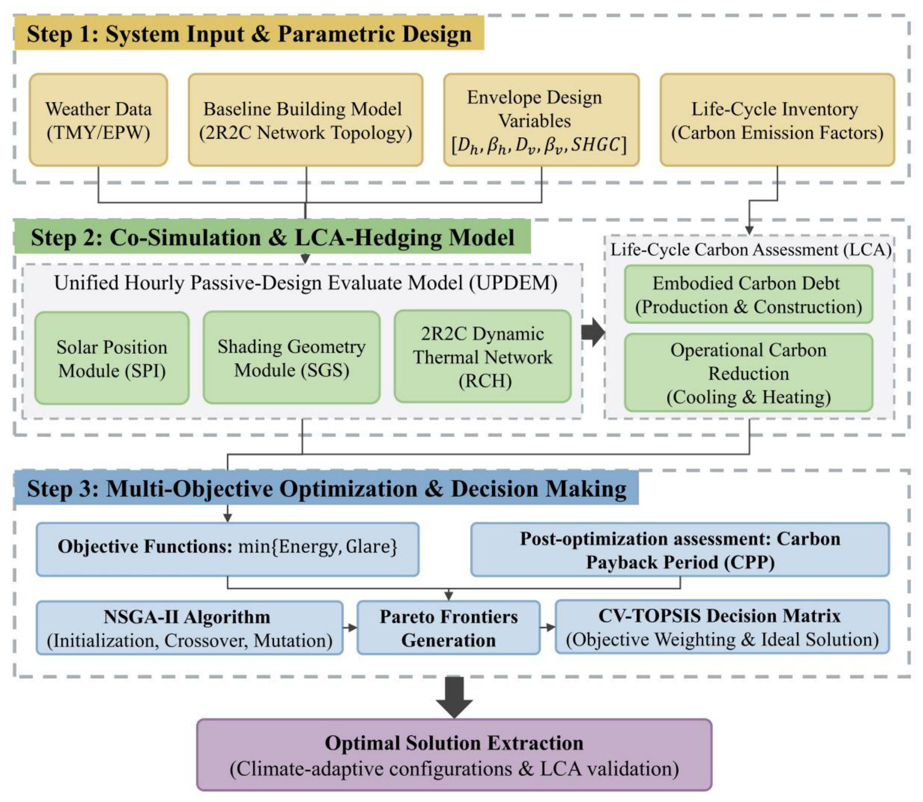
In practical terms, this integration converts each candidate retrofit scheme into directly comparable indicators of operational energy change, transmitted solar exposure response, and carbon payback feasibility. The workflow therefore supports early retrofit decisions by first generating Pareto alternatives, then selecting representative compromises through CV-TOPSIS, and finally checking whether the upfront embodied carbon debt can be offset by B6 operational carbon savings.

The following subsections describe how these modules are linked in the computational workflow, and the overall procedure is summarized in Figure 1.

2.1. The UPDEM Framework

Conventional external shading design often relies on static solar altitude checks at noon on representative summer or winter days. Such simplified checks may underrepresent low-angle morning and evening solar exposure in low-latitude regions, while also overestimating the need for shading in high-latitude regions where winter solar gains are beneficial. UPDEM is introduced to address this mismatch. Using 8760 hourly typical meteorological year (TMY) data, the model links hourly solar-path reconstruction, shading geometry mapping, and coupled solar–thermal response analysis.

2.1.1. Solar Spatiotemporal Geometry and Effective Facade Irradiance Analysis (SPI)

The system first reconstructs the hourly solar trajectory for any given latitude and longitude. For the n-th day of the year, the solar declination angle $\delta \left(n\right)$ and the hour angle $\omega \left(t\right)$, corrected by the apparent solar time, determine the solar altitude angle ${\alpha }_s\left(t\right)$ and azimuth angle at a given time t:

$$sin{\alpha }_s\left(t\right)=sin\varphi ·sin\delta +cos\varphi ·cos\delta ·cos\omega \left(t\right),$$

(1)

where $\varphi$ denotes the local latitude. For a vertical facade ($\beta =90$°) with an orientation azimuth angle of ${\gamma }_f$, the cosine of the incidence angle between the solar ray and the facade normal can be expressed as:

$$cos\theta \left(t\right)=cos{\alpha }_s\left(t\right)·cos({\gamma }_s\left(t\right)-{\gamma }_f),$$

(2)

On this basis, the model uses the global horizontal irradiance (GHI), direct normal irradiance (DNI), and diffuse horizontal irradiance (DHI) from meteorological data and projects the direct, diffuse, and ground-reflected components onto facades of different orientations to obtain the hourly total window irradiance $I_{\mathrm{win}}\left(t\right)$:

$$I_{\mathrm{win}}\left(t\right)=\mathrm{DNI}\left(t\right)·max(0,cos\theta \left(t\right))+I_d\left(t\right)+I_r\left(t\right),$$

(3)

where $I_d\left(t\right)$ and $I_r\left(t\right)$ denote the sky-diffuse and ground-reflected irradiance components incident on the window plane, respectively.

2.1.2. Shading Geometry Dynamics and Dynamic Shading Matrix (SGS)

External shading elements act as geometric screening elements that regulate the solar boundary condition of the building envelope. To keep the optimization variables bounded and numerically stable, the direct shading ratio ($S_o$) and the direct transmittance ratio ($S_{dir}$) are introduced as proxy variables:

$$S_o(t,x)=clip\left({\displaystyle \frac{A_{sh}(t,x)}{A_{win}}},0,1\right),$$

(4)

$$S_{dir}(t,x)=1-S_o(t,x).$$

(5)

Here, x denotes the design vector containing the overhang depth ($d_s$) and the louver tilt angle (${\theta }_s$). To characterize the interception mechanisms of different shading components for radiation in different angular ranges, the horizontal profile angle (HPA) and vertical profile angle (VPA) are used to describe shading effectiveness:

$$tan\left(VPA\left(t\right)\right)={\displaystyle \frac{tan{\alpha }_s\left(t\right)}{|cos(HPA\left(t\right)\left)\right|}}.$$

(6)

Horizontal overhangs mainly constrain the VPA and are effective in intercepting high-angle solar radiation around noon, whereas vertical fins or louvers mainly constrain the HPA and are used to intercept low-angle direct solar radiation from the east and west. The physical interception effect of combined shading is approximated by the product $S_{\mathrm{dir}}(t,x)\approx S_h(t,x)·S_v(t,x)$, which keeps the global optimization computationally tractable. This approximation may introduce errors by neglecting secondary mutual shading, edge effects, anisotropic diffuse radiation, and detailed facade geometry. Its influence is expected to be most visible in transmitted solar exposure and solar gain estimates, especially during low-angle sun periods.

2.1.3. Dynamic Solution of the Building Thermal Resistance–Capacitance Network (RCH)

After the effective transmitted irradiance is obtained, its indoor heat accumulation and dissipation need to be quantified. Conventional simplified steady-state models cannot capture the thermal lag of old masonry or frame residential buildings under large temperature fluctuations. For this reason, the thermodynamic module of UPDEM is extended to a 2R2C dynamic network topology.

In this model, the building is decomposed into an indoor air node ($T_{air}$), representing a fast thermal response, and a thermal mass node ($T_{mass}$), representing a slow thermal response, such as that of concrete slabs or heavyweight brick walls. The transient heat balance is governed by the following coupled differential equations:

$$C_{mass}{\displaystyle \frac{d{T}_{mass}}{dt}}=Q_{rad\_solar}\left(t\right)+H_{in}(T_{air}-T_{mass}),$$

(7)

$$C_{air}{\displaystyle \frac{d{T}_{air}}{dt}}=Q_{conv\_solar}\left(t\right)+Q_{int}\left(t\right)+U{A}_{env}(T_{out}-T_{air})+H_{in}(T_{mass}-T_{air}).$$

(8)

Here, $C_{\mathrm{mass}}$ denotes the thermal capacitance associated with the envelope structure and represents the heat-storage capacity of the building. $Q_{rad\_solar}$ and $Q_{conv\_solar}$ denote the components of solar heat gains allocated to long-wave radiative heat transfer and convective heat transfer, respectively. $U{A}_{env}$ denotes the external heat-loss coefficient. To balance the computational efficiency required for long-term simulations with the repeated model evaluations required in multi-objective optimization, the coupled ordinary differential equations are discretized and solved using the explicit forward Euler method. The time step is set to $\Delta t=1$ h, based on which the hourly cooling load $Q_{cool}\left(t\right)$ and heating load $Q_{heat}\left(t\right)$ required to maintain the indoor set-point temperature $T_{set}$ are calculated. The 2R2C representation and 1 h forward Euler scheme simplify multi-zone heat transfer, envelope layering, air mixing, and short-term peak dynamics. Therefore, they may smooth peak loads and slightly shift load timing, but they remain appropriate for annual screening under hourly TMY inputs.

2.2. Life-Cycle-Informed Carbon Payback Assessment

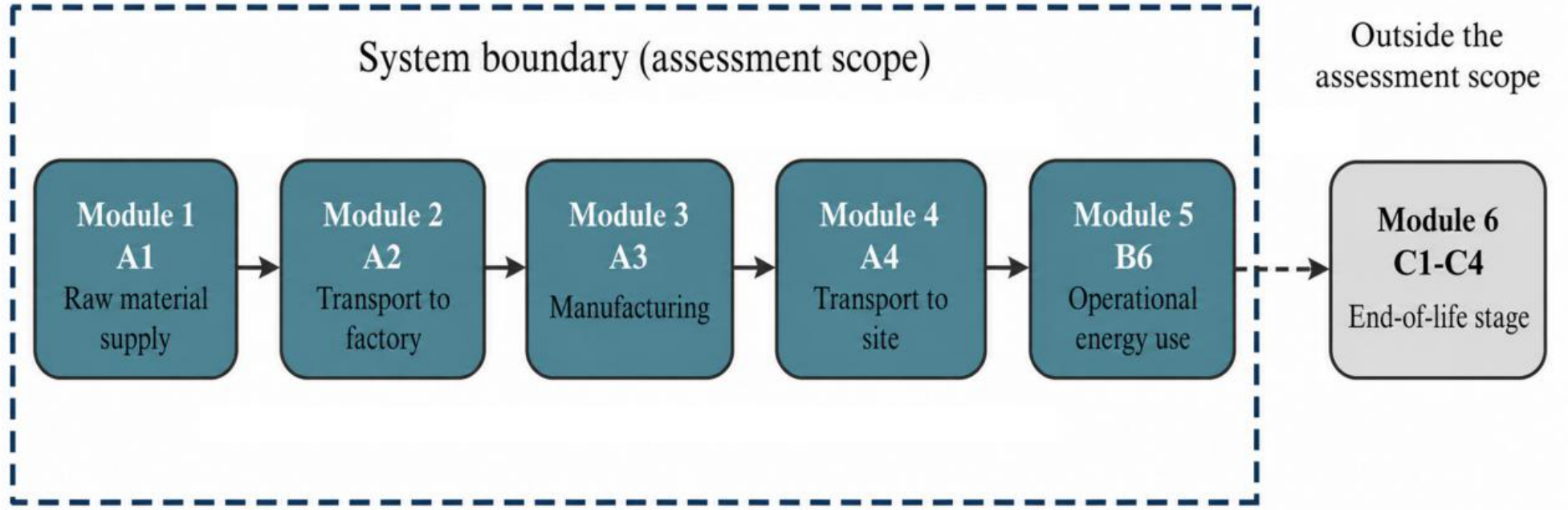
Operational energy savings alone may overestimate the environmental benefit of passive shading retrofits because additional materials, such as aluminum shading components and Low-E glazing, introduce upfront embodied carbon. A life-cycle-informed carbon boundary is used to evaluate the balance between upfront carbon emissions and subsequent operational carbon reductions. Following the modular logic of EN 15978 and the life-cycle assessment principles of ISO 14040/14044, the system boundary includes material production stages A1–A3 and pre-construction transport stage A4. The operational stage is represented by B6 energy use. Figure 2 summarizes this boundary and the corresponding calculation logic. End-of-life processes, maintenance, replacement, and module D benefits are intentionally excluded to maintain a conservative and reliable estimate. Given that the target pre-2000 residential buildings have a limited remaining service life (typically 20–30 years), passive aluminum components and new glazing systems are unlikely to require major replacements (B4 stage) before building demolition. Furthermore, maintenance (B2 stage) involves negligible energy input. Although omitting the significant recycling potential of aluminum (Module D) excludes substantial carbon credits, it ensures that the calculated upfront carbon debt is not overly optimistic.

The embodied carbon calculation includes the main shading and glazing materials listed in

Table 1. Basic data used for embodied carbon accounting of major retrofit materials.

Material/Component Type	Density	Embodied Carbon Emission Factor, ${\mathit{EF}}_{\mathbf{mat}}$	Data Source
Aluminium alloy profile for shading louvers/fins	2700 kg/m3	18.10 kg CO2e/kg	GB/T 51366-2019 [4]
Ordinary single clear glass for baseline windows	2500 kg/m3	1.19 kg CO2e/kg	GB/T 51366-2019 [4]
Low-E glass for retrofit replacement windows	2500 kg/m3	1.45 kg CO2e/kg	ICE database [51]

and assumes no additional primary structural reinforcement at the screening stage. Project-specific interventions such as structural reinforcement, special anchorage, supporting subframes, or wall repair are excluded from the current boundary. If such interventions are required after structural appraisal, their material quantities and embodied carbon should be added to the A1–A4 inventory, which would lengthen the resulting CPP.

Within this boundary, the carbon performance of each retrofit scheme is evaluated by two indicators: net carbon reduction over the remaining service life and Carbon Payback Period (CPP). The CPP is not included as an objective function in the genetic algorithm. Instead, it is used after Pareto optimization to interpret whether the selected retrofit configuration can recover its upfront carbon burden through annual operational carbon savings.

$$\Delta C_{net}={\displaystyle \sum _{y=1}^{N_{life}}}(E_{base,y}-E_{opt,y})·E{F}_{grid}-\sum _j(M_j·E{F}_{mat,j}),$$

(9)

where $E_{base,y}$ and $E_{opt,y}$ denote the annual equivalent electricity consumption under the baseline and retrofit scenarios, respectively (kWh); $E{F}_{grid}$ is the regional grid carbon emission factor of the provincial power grid in each climatic region (kg CO₂e/kWh), which reflects the spatial heterogeneity between coal-dominated power systems in northern China and the higher share of clean energy in southern China; $M_j$ is the quantity of the j-th shading or envelope material; ${EF}_{mat,j}$ is the corresponding life-cycle carbon emission factor; and $N_{life}$ is the remaining service life of the retrofitted building.

To provide a direct screening indicator for payback feasibility, CPP is calculated as:

$$CPP=\left\{\begin{array}{c}\hfill {\displaystyle \frac{{\sum }_j(M_j·E{F}_{mat,j})}{(E_{base}-E_{opt})·E{F}_{grid}}},\Delta E>0\\ \hfill Notachieved,\Delta E\le 0\end{array}\right..$$

(10)

For reproducibility, the unit mass and embodied carbon emission factors ($E{F}_{mat}$) of the retrofit materials are specified using the Standard for Building Carbon Emission Calculation (GB/T 51366-2019) [4] and the relevant literature, as listed in Table 1.

2.3. Multi-Objective Optimization Setup

Passive shading retrofit is a nonlinear multi-objective problem. Increasing shading depth and reducing SHGC can reduce summer solar heat gains and cooling loads, but they may also reduce transmitted solar radiation and useful winter solar gains. To evaluate this trade-off, the optimization workflow couples NSGA-II with a multi-criteria decision-making procedure and uses annual equivalent energy demand and a transmitted solar exposure proxy as the main performance indicators. The proxy is introduced to retain a direct physical link between shading interception, transmitted solar heat gain, and solar exposure reduction within the UPDEM workflow. It is therefore intended for comparative screening of radiative exposure and solar gain trade-offs, not for predicting daylight availability, glare probability, or visual comfort in the sense of established daylighting metrics.

2.3.1. Construction of a Multi-Objective Optimization Model (MOO)

Let $x\in \mathsf{\Omega }$ denote the retrofit design vector within the feasible solution space. The vector includes shading depth, shading angle, and glazing SHGC. The optimization problem is formulated to minimize annual equivalent energy demand and low-transmitted-irradiance hours, while constraining excessive transmitted irradiance during occupied periods:

$$\begin{array}{c}\underset{x\in \mathsf{\Omega }}{min}f\left(x\right)={[E_{ann}\left(x\right),H_{low}\left(x\right)]}^T,\\ s.t.H_{high}\left(x\right)\le 5\%.\end{array}$$

(11)

Here, $E_{ann}\left(x\right)$ is the annual equivalent energy demand, calculated as the sum of annual cooling and heating demand. $H_{low}\left(x\right)$ denotes the number of occupied hours during which indoor transmitted solar irradiance is below the lower threshold. $H_{high}\left(x\right)$ denotes the occurrence rate of transmitted irradiance above the upper threshold.

Indoor transmitted solar irradiance is used as a transmitted solar exposure proxy to maintain a consistent physical basis between solar gain calculation and optimization [8]. Occupied hours with transmitted irradiance below 15 W/m² are counted as low-transmitted-irradiance hours, while hours above 250 W/m² are treated as high-transmitted-irradiance exposure. These two values are not adopted as universal human visual comfort or glare thresholds. Instead, they are used as internal screening thresholds in the same radiometric unit as the solar heat gain calculation: the lower bound identifies hours with very limited transmitted solar radiation, whereas the upper bound limits cases with strong direct solar exposure during occupied periods. Classical daylight and glare indicators, including UDI, DGI, DGP, sDA, and ASE, are based on illuminance-, luminance-, or glare-probability formulations and therefore cannot be directly converted from the W/m²-based transmitted irradiance proxy without additional optical, geometric, sky condition, and view direction assumptions [12,13,14,15]. Accordingly, the corresponding results should be read only as screening-level transmitted solar exposure comparisons, not as daylight-autonomy, glare risk, or full visual comfort evaluations. Detailed design application would still require dedicated daylight and glare simulation using established photometric and luminance-based metrics.

The NSGA-II settings were chosen to support Pareto-front convergence while maintaining solution diversity. The population size was 100 and the maximum number of generations was 150. Simulated binary crossover (SBX) was used with a crossover probability of 0.9 and a distribution index of ${\eta }_c=15$. Polynomial mutation (PM) was used with a mutation probability of 0.1 and a distribution index of ${\eta }_m=20$.

2.3.2. Selection of the CV-TOPSIS Trade-Off Solution

The Pareto-front provides a set of non-dominated alternatives rather than a single optimum. To select a representative solution for cross-climate comparison, the coefficient of variation (CV) weighting method is combined with TOPSIS. The CV method is used to derive objective weights from the dispersion of the Pareto solutions. A weighted normalized decision matrix is then constructed, and the positive ideal solution is defined as the alternative with lower annual energy demand and fewer transmitted solar exposure proxy hours.

The relative closeness coefficient is calculated for each candidate solution. The solution with the highest coefficient is selected as the CV-TOPSIS trade-off solution. This solution is used for engineering interpretation and comparison; it should not be interpreted as an absolute optimum.

First, the objective weights $w_j$ are calculated from the statistical dispersion of each objective function within the Pareto set:

$$\begin{array}{c}C{V}_j={\displaystyle \frac{{\sigma }_j}{{\mu }_j}},\\ w_j={\displaystyle \frac{C{V}_j}{{\sum }_{k}C{V}_k}}.\end{array}$$

(12)

Subsequently, a weighted normalized decision matrix is constructed. The positive ideal solution ($Z^{+}$), representing the lowest energy demand and the lowest low-transmitted-irradiance hours, and the negative ideal solution ($Z^{-}$) are then identified in the solution space. The Euclidean distances from each candidate solution i to the positive and negative ideal solutions are calculated, and the relative closeness coefficient $C_i$ is obtained as follows:

$$C_i={\displaystyle \frac{D_i^{-}}{D_i^{+}+D_i^{-}}}.$$

(13)

By selecting the candidate with the highest $C_i$ score, the procedure identifies a representative compromise between lower annual energy demand and reduced low-transmitted-irradiance hours. This solution is used for cross-climate engineering interpretation and should not be interpreted as a universal optimum. It also does not imply that no other energy-saving alternatives exist within the same regional Pareto set.

Because CV-TOPSIS is one compromise-selection rule, the decision sensitivity of the recommendations was examined against alternative decision preferences, including equal weighting, energy-prioritized TOPSIS ($w_E=0.7,w_H=0.3$), exposure-prioritized TOPSIS ($w_E=0.3,w_H=0.7$), and a VIKOR-type compromise-ranking logic [49,50]. These checks do not change the Pareto-front itself; they test whether the engineering interpretation is driven mainly by climate-dependent physical response or by the final ranking rule.

3. Case Studies

The case-study design is intended to test whether the proposed retrofit screening logic remains consistent across substantially different climates. Instead of focusing on a single climatic zone, the analysis compares typical existing residential buildings across several geographical regions of China and links the resulting design choices to life-cycle carbon reduction potential.

3.1. Climatic Zones and Representative Cities

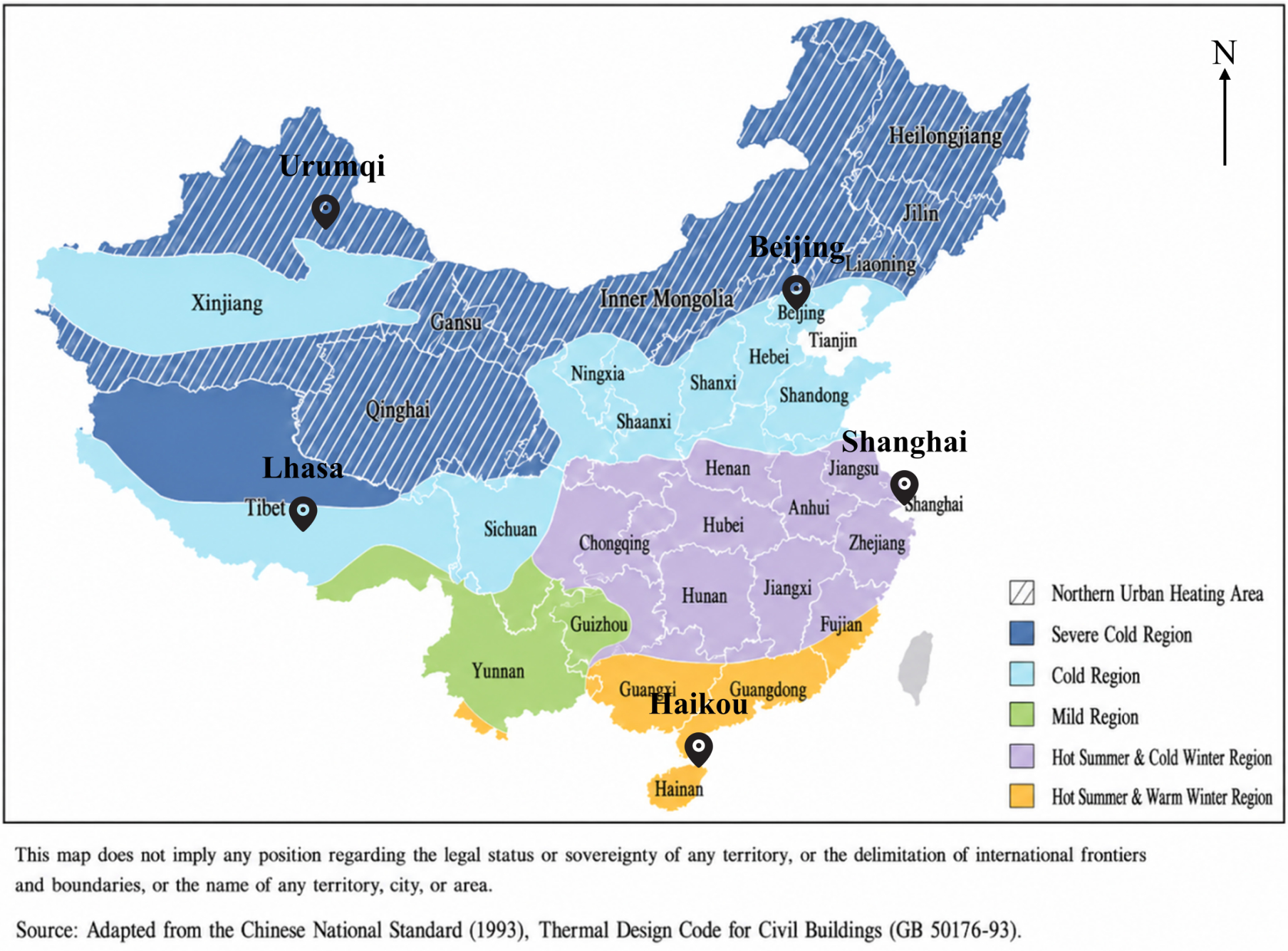
China spans a wide range of climatic conditions, and regional climate differences directly determine the dominant patterns of building heating and cooling loads. According to the Code for Thermal Design of Civil Buildings (GB 50176-2016) [5], Haikou, Shanghai, Beijing, Lhasa, and Urumqi were selected as representative reference cities for the five typical climatic regions.

As shown in

Table 2. Geographical and climatic characteristics of the representative cities.

City	Latitude	Longitude	Climate Region [5]	HDD [5]	CDD [5]	Retrofit Challenge
Haikou	20.03° N	110.32° E	Hot Summer and Warm Winter region	0	450~550	Cooling-dominated; strong solar control required.
Shanghai	31.23° N	121.47° E	Hot Summer and Cold Winter region	1600~1800	150~250	Balance between summer shading and winter solar gain.
Beijing	39.90° N	116.40° E	Cold region	2800~3000	100~150	Seasonal conflict between cooling reduction and heating demand.
Lhasa	29.65° N	91.11° E	Severe Cold region	3000~3200	0~10	Strong radiation with heating-dominated demand.
Urumqi	43.82° N	87.61° E	Cold region	4500~4800	30~50	Heating preservation; excessive shading should be avoided.

, the five cities exhibit distinct seasonal thermal conflicts. Haikou receives high solar radiation throughout the year and is predominantly cooling-driven. Urumqi, by contrast, has long and extremely cold winters, so heating preservation dominates even though summer solar protection is still needed. This climatic heterogeneity provides a broad comparative test of the proposed multi-objective optimization framework (UPDEM). Lhasa is treated as a high-altitude, heating-dominated, high-radiation case to represent the Qinghai–Tibet Plateau climatic context within the broader severe cold classification.

Figure 3 maps the locations of the representative cities and their climatic zoning.

3.2. Reference Building Prototype Settings

A large share of China’s aging urban residential stock was built before the end of 2000, when envelope thermal requirements and external solar control measures were generally less stringent than in current codes. Buildings from this period commonly lack external shading and have weak envelope thermal performance, making them representative candidates for energy-saving retrofit screening.

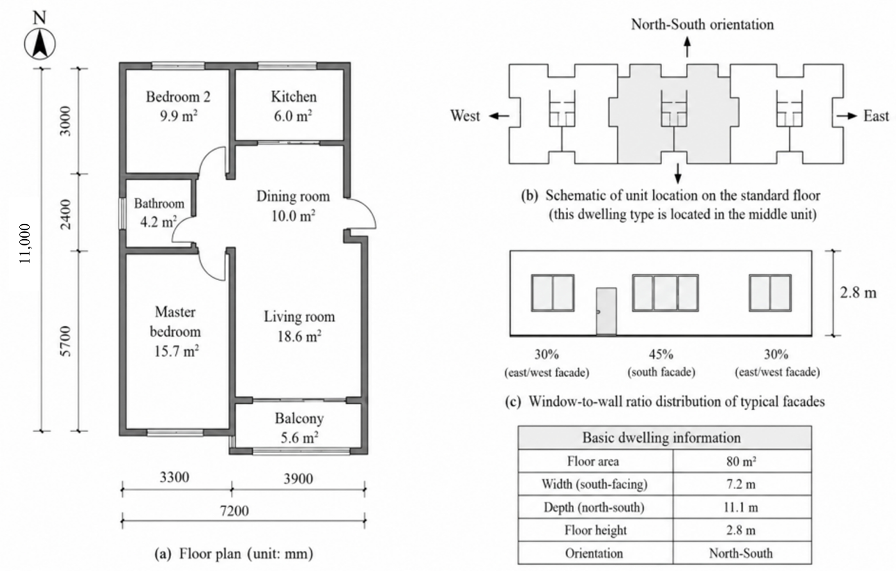
The model uses a typical 80 m² north–south-oriented residential unit commonly found in old urban communities as the simulation prototype, as shown in Figure 4. Based on the reference layout and early residential design standards, the areas most exposed to direct solar radiation are identified as the south-facing main facade, with a window-to-wall ratio of approximately 45%, and the east- and west-facing bedrooms, with a window-to-wall ratio of approximately 30%. The baseline building adopts uninsulated brick–concrete exterior walls and ordinary single clear glazing, which may increase indoor overheating risk and air-conditioning electricity use in summer. The main thermal parameters and operating boundaries used in the UPDEM dynamic thermal response module are listed in

Table 3. Thermal parameters and operating boundaries of the reference residential model.

Component/Parameter	Specification and Physical Input Value
Exterior wall U-value	2.0 W/(m2·K) (Typical uninsulated 240 mm solid brick wall)
Roof U-value	1.5 W/(m2·K) (Uninsulated concrete roof slab)
Overall envelope heat conductance ($U{A}_{env}$)	180.0 W/K (Derived equivalent parameter representing the lack of insulation commonly found in old brick–concrete buildings)
Building thermal mass ($C_{mass}$)	$7.0\times {10}^6$ J/K, representing the high thermal capacity of brick walls and concrete slabs
Indoor air heat capacity ($C_{air}$)	$4.2\times {10}^5$ J/K
Indoor convective heat-transfer coefficient ($H_{in}$)	470.0 W/K
Baseline window	Ordinary single clear glazing (SHGC: 0.75, U-value: 5.8 W/(m2·K)), without external shading
Shading component geometry	Effective cross-sectional thickness of 1.5 mm (Aluminum alloy, used for embodied carbon material volume calculation)
Internal heat gains ($Q_{int}$)	Constant equivalent internal heat gain of 300 W for the 80 m2 reference unit, corresponding to 3.75 W/m2. This value represents a continuous aggregate of occupant, lighting, and plug-load gains for comparative screening.
HVAC control set points and schedules	Cooling is activated when indoor air temperature exceeds $T_{set,cool}=24$ °C; heating is activated when indoor air temperature falls below $T_{set,heat}=18$ °C. These values are used as reference thermostatic thresholds under 24-h continuous control, rather than as measured occupant thermostat settings.

.

The HVAC set points and internal heat gains were defined as reference operating boundaries rather than measured occupant behavior profiles. The cooling and heating thresholds of 24 °C and 18 °C were selected as simplified thermostatic limits consistent with commonly used indoor design-temperature assumptions in Chinese civil-building HVAC design practice [53]. In the 2R2C model, these values are used to determine the activation of active cooling and heating, rather than to represent surveyed thermostat preferences in real households.

The internal heat gain was set to a constant 300 W for the 80 m² reference unit, corresponding to 3.75 W/m². This value was used as a continuous equivalent aggregate of occupant, lighting, and plug-load heat gains. A constant equivalent gain was adopted to maintain consistent boundary conditions across the five climatic regions and to isolate the effects of shading geometry and glazing properties. It should not be interpreted as a time-varying residential occupancy or appliance-use schedule.

The 80 m² unit is used as an archetypal screening prototype for pre-2000 urban residential buildings, rather than as a statistically complete representation of China’s entire housing stock. It captures common retrofit-relevant features of this stock segment, including a compact apartment layout, north–south orientation, brick–concrete construction, weak envelope insulation, ordinary single glazing, and the absence of external shading.

Variations in building typology, floor level, orientation, window-to-wall ratio, wall and roof thermal properties, thermal mass, infiltration, occupancy density, internal gains, HVAC set points, and operating schedules may change absolute energy savings, Pareto-solution rankings, and carbon payback values. Therefore, the numerical results should be transferred cautiously. The more robust output is the climate-dependent design tendency under consistent assumptions, while project-specific application requires recalibration with local archetype, envelope, occupancy, and HVAC operation data.

3.3. Definition of the Optimization Variable Space

For older residential communities, practical retrofit schemes should avoid major structural intervention. The decision variables ($\mathbf{x}\in \mathsf{\Omega }$) are limited to the geometry of external facade-mounted shading components and the optical–thermal properties of replacement windows; the original building form and window areas remain unchanged.

The geometrical ranges in

Table 4. Optimization design variables and value ranges for the NSGA-II algorithm.

Variable Symbol	Physical Meaning	Value Range	Variable Type
$d_S$	South-facing horizontal overhang depth (m)	[0.00, 2.00]	Continuous
${\theta }_S$	South-facing horizontal overhang tilt angle (°)	[0, 45]	Continuous
$d_N$	North-facing rear-facade horizontal overhang depth (m)	[0.00, 1.50]	Continuous
${\theta }_N$	North-facing rear-facade horizontal overhang tilt angle (°)	[0, 45]	Continuous
$d_{EW}$	East–west vertical louver/fin depth (m)	[0.00, 1.50]	Continuous
${\theta }_{EW}$	East–west vertical louver tilt angle (°)	[0, 90]	Continuous
SHGC	Solar heat gain coefficient of replacement glazing	[0.20, 0.85]	Continuous

are screening-level parametric bounds rather than directly buildable prescriptions. For pre-2000 brick–concrete residential buildings, large overhangs or deep louver systems require project-level checks of residual load-bearing capacity, anchorage safety, wind-load resistance, deterioration state, and construction quality before implementation [54,55]. Therefore, the optimized geometries should be interpreted as performance-screening candidates subject to subsequent structural verification, not as final construction details.

In terms of physical mechanism, south-facing horizontal overhangs mainly control the vertical profile angle and reduce high-angle solar radiation around noon. East- and west-facing fins or louvers mainly control the horizontal profile angle and reduce low-angle direct solar exposure in the morning and late afternoon. In addition, SHGC is treated as a continuous glazing parameter to investigate the balance between solar gain control, winter heat gain preservation, and the transmitted solar exposure proxy. The decision-variable ranges used in the NSGA-II optimization are listed in Table 4.

3.4. Benchmark Comparison of the Reduced-Order Model

To overcome the limitations of coupling high-fidelity whole-building simulation engines directly with evolutionary algorithms, this study embeds a reduced-order 2R2C thermal network within the UPDEM framework. Direct co-simulation with EnergyPlus for optimization faces substantial bottlenecks: the NSGA-II setup in this study requires 15,000 evaluations per climatic region. Repeatedly invoking EnergyPlus via external scripts incurs extensive file I/O operations and initialization overhead, making multi-city batch optimization computationally prohibitive. Furthermore, integrating the highly customized spatiotemporal shading geometry algorithm (SGS) dynamically with whole-building engines requires complex stepwise co-simulation, which limits computational robustness. Therefore, a reduced-order model explicitly solved in a unified mathematical environment is adopted to ensure that the optimization loop remains highly efficient, numerically stable, and fit-for-purpose for screening-level comparative analysis [36]. Rather than seeking full validation against field measurements, this section aims to verify whether the reduced-order model can adequately reproduce the primary cooling load dynamics of a reference EnergyPlus dataset with acceptable statistical agreement. An open residential load profile dataset published on Mendeley Data was used as the benchmark [56]. The weather boundary condition was kept consistent with the benchmark case, using the Newark TMY3 weather file, to avoid discrepancies caused by different external climate inputs.

A single-zone 2R2C model inevitably simplifies the heat-storage distribution, internal zoning, and load aggregation of a multi-zone residential building. Direct comparison with the benchmark loads may introduce scale-related deviations, so gray-box parameter identification was adopted to calibrate the key thermal parameters of the 2R2C network [36]. A differential evolution algorithm was used to identify the equivalent thermal resistances and capacitances listed in

Table 5. Parameter identification results for the 2R2C model.

Parameter Symbol	Physical Meaning	Identified Value	Unit
$R_1$	Equivalent thermal resistance between indoor air and the interior wall surface	$2.14\times {10}^{-3}$	K/W
$R_2$	Equivalent thermal resistance between wall conduction and the outdoor environment	$6.85\times {10}^{-3}$	K/W
$C_{air}$	Equivalent heat capacity of indoor air and indoor contents	$4.20\times {10}^5$	J/K
$C_{mass}$	Equivalent heat capacity of the building envelope thermal mass	$7.00\times {10}^6$	J/K
Phase-lag	Thermal phase-lag time	3.2	h

. A 7.2 h moving-average window was further introduced to approximate the delayed response associated with air mixing and thermal mass [57]. In addition, the internal heat gain schedule was represented by two load levels, 2737 W during daytime and 1384 W at night, and a linear scaling procedure was applied to align the load magnitude with the benchmark dataset.

Since the primary thermal effect of external shading is associated with reducing solar heat gains and cooling demand [8], the benchmark comparison focuses on the main cooling season from June to September. Data points with very low loads, defined as less than 5% of the peak load, were excluded to reduce the influence of transition-season noise and non-cooling end uses. This filtering step was applied only for the calibration and benchmark comparison exercise and does not imply that the model fully represents all seasonal operating modes.

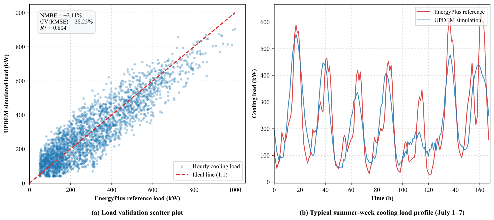
The model discrepancy was evaluated using the calibration statistics recommended in ASHRAE Guideline 14 [58]. As shown in Figure 5, the calibrated UPDEM model shows acceptable agreement with the EnergyPlus benchmark loads for the selected cooling season period. The normalized mean bias error (NMBE) is +2.11%, and the coefficient of variation of the root mean square error (CV(RMSE)) is 28.25%, both falling within the commonly used hourly calibration thresholds. The coefficient of determination is 0.804, indicating that the reduced-order model captures a substantial portion of the temporal variation in the benchmark cooling load profile.

These benchmark results support the use of the calibrated 2R2C model for screening-level comparison of passive shading alternatives within the defined modeling boundary. The comparison is still based on an EnergyPlus benchmark dataset, not on field measurements from the five Chinese residential prototypes. The resulting energy estimates are used primarily as relative performance indicators for comparing retrofit options, rather than as absolute predictions of measured building energy use. Thus, the predictive capability claimed here is relative and screening-oriented: the model is intended to preserve the dominant solar–thermal response needed to rank alternatives under consistent assumptions, while reducing the computational burden that would arise from repeated high-fidelity co-simulation. The remaining modeling error can propagate in three ways. First, annual energy predictions may deviate from measured performance because peak loads and short-term thermal responses are simplified. Second, Pareto-front positions and CV-TOPSIS rankings may change for alternatives with very similar objective values, although broad climate-dependent tendencies are less sensitive to small ranking changes. Third, carbon payback estimates inherit uncertainty from annual electricity savings; therefore, cases with small savings or negative savings should be interpreted more cautiously than cases with large savings and short payback periods.

4. Results and Discussion

4.1. Optimization Dynamics and Pareto-Front Analysis

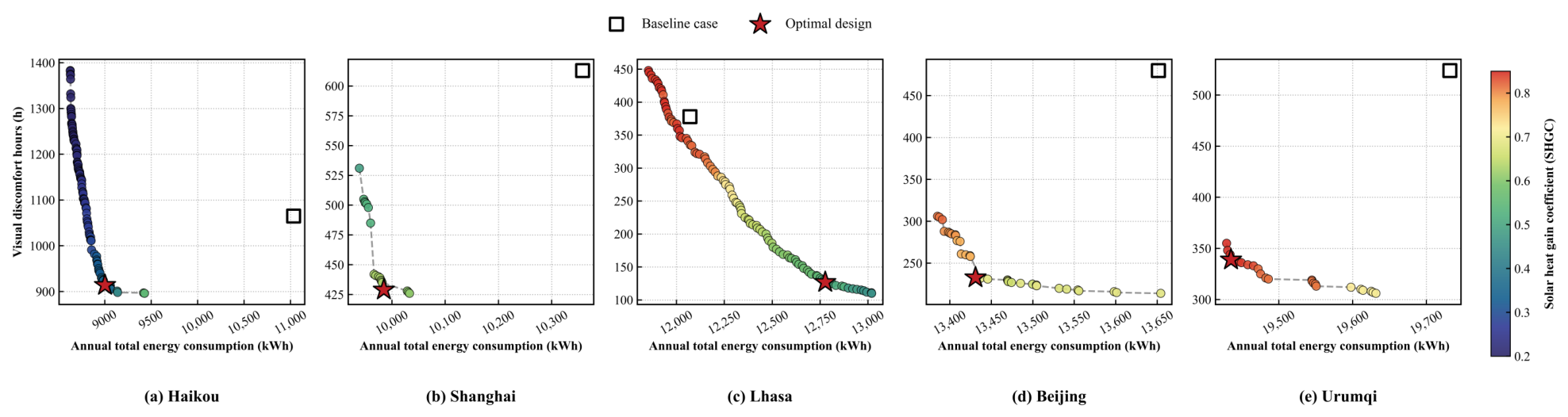
External shading design involves trade-offs among summer solar control, winter solar gain preservation, and transmitted solar exposure performance. NSGA-II was applied independently to the five representative climatic regions using seven envelope-related variables, including shading geometry and glazing SHGC. The Pareto fronts in Figure 6 show that climatic heterogeneity constrains the feasible performance space of passive shading retrofits.

In cooling-dominated climates like Haikou, adopting lower SHGCs and deeper shading configurations significantly reduces energy demand while incurring only a marginal heating penalty. This produces a wider Pareto distribution. In Urumqi, by contrast, annual performance is heating-dominated, and excessive shading reduces useful winter solar gains. The Pareto-front therefore becomes steeper, indicating a stronger conflict between annual energy demand and transmitted solar exposure control.

4.2. Climate-Dependent Morphology of Selected Trade-Off Solutions

Based on the CV-TOPSIS decision procedure, one compromise retrofit solution was selected from the Pareto set for each climatic region. These solutions balance annual energy demand and the transmitted solar exposure proxy within the defined decision framework. The seven envelope-related design variables and the corresponding energy and carbon payback indicators are summarized in

Table 6. CV-TOPSIS-selected trade-off solutions for the five representative cities.

Representative City	South-Facing Facade		North-Facing Facade		East–West-Facing Facades		Glazing
	${\mathit{d}}_{\mathit{S}}$ (m)	${\mathit{\theta }}_{\mathit{S}}$ (°)	${\mathit{d}}_{\mathit{N}}$ (m)	${\mathit{\theta }}_{\mathit{N}}$ (°)	${\mathit{d}}_{\mathit{EW}}$ (m)	${\mathit{\theta }}_{\mathit{EW}}$ (°)	SHGC
Haikou	0.79	14	0.57	32.7	1.47	85	0.36
Shanghai	0.86	0.2	1.36	38.9	1.12	60.7	0.6
Lhasa	0	1.1	1.49	43.4	0.06	41.7	0.52
Beijing	0.55	0.3	1.49	40.5	1.37	77.9	0.69
Urumqi	0.66	1.4	1.22	13.6	1.33	84.3	0.85

and

Table 7. Comprehensive energy-saving and carbon payback indicators for the selected trade-off solutions.

Typical City	Base Energy Consumption (kWh/yr)	Annual Electricity Savings $\mathbf{\Delta }\mathit{E}$ (kWh/yr)	Overall Energy Saving Rate ${\mathit{\eta }}_{\mathit{E}}$ (%)	Upfront Embodied Carbon (kg CO2e)	Carbon Payback Period, CPP (yr)	Change in Solar Exposure Proxy Hours $\mathbf{\Delta }{\mathit{H}}_{\mathit{proxy}}$ (h)
Haikou	11,034.2	2030.3	18.40	1644.5	1.8	−151
Shanghai	10,372.2	373.4	3.60	392.1	2.5	−184
Lhasa	12,070.1	−706.1	−5.85	58.2	N.A.	−251
Beijing	13,611.1	220.5	1.62	598.0	4.8	−247
Urumqi	19,766.7	296.5	1.57	1160.2	6.5	−185

Note: N.A. = not achieved because $\Delta E\le 0$.

. Therefore, the following interpretation refers to the selected compromise solutions, not to all feasible Pareto alternatives. The alternative weighting and compromise-ranking checks indicate that the broad climate-dependent tendencies are more robust than the exact selected parameter values. Haikou consistently favors stronger solar control and lower SHGC, whereas Beijing and Urumqi consistently favor higher SHGC and restrained south-facing shading to preserve winter gains. Shanghai and Lhasa are more sensitive to the decision framework because their Pareto sets involve stronger energy–exposure trade-offs.

Table 6 shows that the selected window and shading configurations differ markedly by climate. These morphological variations stem from three distinct physical mechanisms:

1.

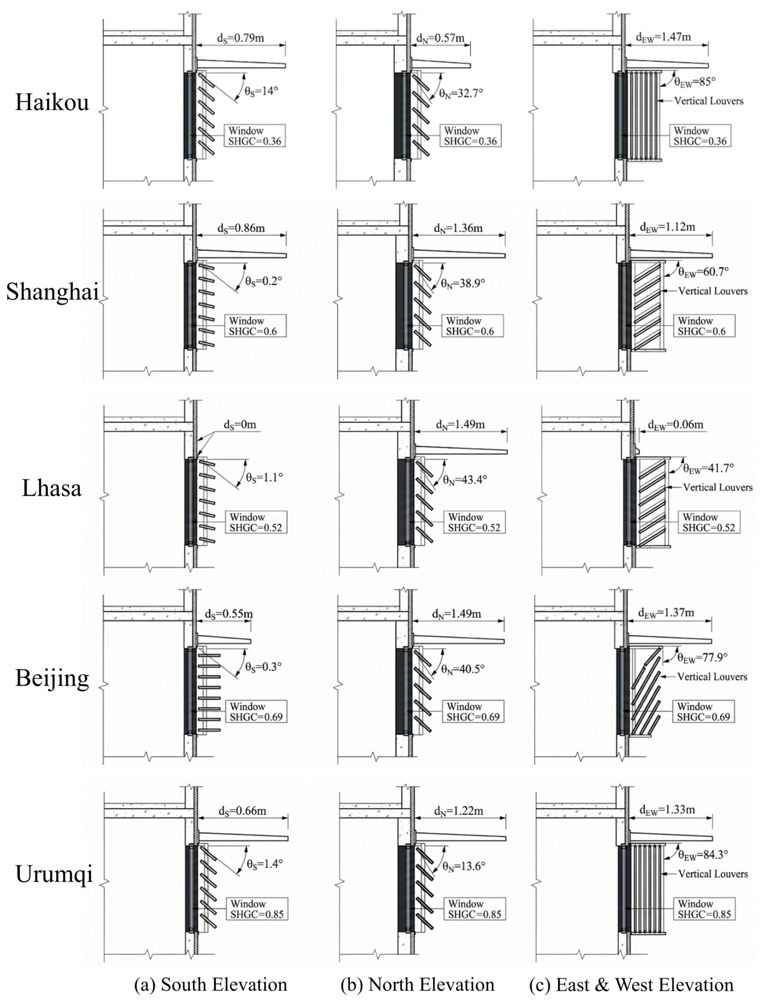
Low-latitude, high-radiation regions: The primary strategy is to strengthen solar radiation control. In Haikou, the selected solution adopts the lowest glazing solar heat gain coefficient (SHGC = 0.36) and deep east–west vertical shading ($d_{EW}=1.47$ m, ${\theta }_{EW}={85}^{\circ }$). This configuration reduces strong low-angle direct solar radiation in the morning and late afternoon, leading to an annual electricity saving of 2030.3 kWh/yr, or 18.4%. In Shanghai, where both summer cooling and winter heating are relevant, the selected SHGC increases to 0.60, reflecting a more balanced strategy between summer solar rejection and winter solar gain utilization.

2.

Heating-dominated northern regions: The selected solutions preserve higher solar transmittance while limiting south-facing fixed overhangs. Beijing and Urumqi retain relatively high SHGC values of 0.69 and 0.85, respectively, to preserve useful winter solar gains. Their south-facing horizontal overhangs remain moderate, with depths of 0.55 m and 0.66 m, whereas east–west shading is still selected to control low-angle solar exposure. Although the annual electricity savings are modest, the selected solutions still achieve positive savings of 220.5 kWh/yr and 296.5 kWh/yr, respectively.

3.

High-altitude, cold, and high-radiation regions: The selected solution reflects a trade-off in which exposure reduction is achieved at the expense of energy performance. For Lhasa, the CV-TOPSIS solution reduces the transmitted solar exposure proxy but incurs an annual energy penalty of 706.1 kWh/yr. Consequently, the CPP is unattainable within the defined A1–A4 + B6 boundary. This result reflects the specific conflict in high-altitude heating-dominated regions: strong solar radiation increases the need for exposure control, whereas winter solar gains remain valuable for reducing heating demand. The Lhasa result should therefore be interpreted as an exposure reduction trade-off for the selected CV-TOPSIS compromise solution, not as evidence that all possible shading configurations in Lhasa increase energy use or lack carbon-saving potential.

This finding also indicates that fixed passive shading is not necessarily the most appropriate first-choice strategy for high-altitude, heating-dominated regions. In such climates, the same fixed geometry that suppresses excessive solar exposure can also block valuable winter solar gains. Movable, retractable, or dynamically controlled shading systems may therefore provide a more suitable alternative, because they can remain open during heating-dominated periods to preserve solar heat gains and be deployed only during periods of excessive solar exposure, overheating risk, or glare risk [10,11]. This seasonal and operational flexibility is not captured by the fixed shading design variables used in the present optimization.

Figure 7 translates these numerical choices into facade sections, making the spatial morphological differences among climatic regions more explicit.

The reconstructed facade sections in Figure 7 illustrate the geometric implications of the selected compromise solutions. The variation in shading depth, louver angle, and SHGC across the five cities suggests that passive shading retrofits should be adapted to local heating–cooling balance and solar-path characteristics, rather than being specified through a uniform envelope rule.

4.3. Spatial Trade-Offs in Carbon Payback Assessment

When the assessment boundary is extended from operational energy to life-cycle-informed carbon performance, passive external shading retrofits reveal a trade-off between upfront embodied carbon burdens and subsequent operational carbon savings. Materials such as aluminum shading components and Low-E glazing introduce additional upfront carbon from production and transport. Therefore, the carbon payback calculation must account for both the embodied carbon of retrofit measures and the regional grid carbon emission factor.

After introducing the carbon payback period (CPP) model, the offsetting calculation must incorporate the regional grid carbon emission factors of provincial power grids in different regions, as listed in

Table 8. Provincial grid carbon emission factors used for carbon payback assessment.

Representative City	Regional Power Grid	Regional Grid Carbon Emission Factor (kg CO2e/kWh)	Energy-Structure Feature
Haikou	Hainan grid (Southern China)	0.450	Relatively high share of nuclear and clean energy
Shanghai	Shanghai grid (East China)	0.420	Influenced by imported clean electricity
Beijing	Beijing grid (North China)	0.565	Coal-dominated, with increasing imported green electricity
Urumqi	Xinjiang grid (Northwest China)	0.602	High-carbon power structure dominated by coal
Lhasa	Tibet grid	0.150	Low-carbon structure dominated by hydropower and photovoltaics

Note: These factors are used as regional average grid carbon emission factors for screening-level carbon payback assessment, not as marginal emission factors. Data source: [59].

[59].

These factors were taken from the official regional average grid emission factors issued by the Ministry of Ecology and Environment in 2023 for the 2023–2025 reporting and verification period [59]. They are used here as static screening factors rather than year-specific marginal or forecast emission factors. Because the source provides reporting-period factors rather than annual dynamic grid decarbonization trajectories, cross-year CPP validation was not performed. Instead, the possible influence of grid-factor variation is examined through the $\pm 20\%$ sensitivity analysis, and future planning applications should adopt annual or scenario-based grid emission factors when available.

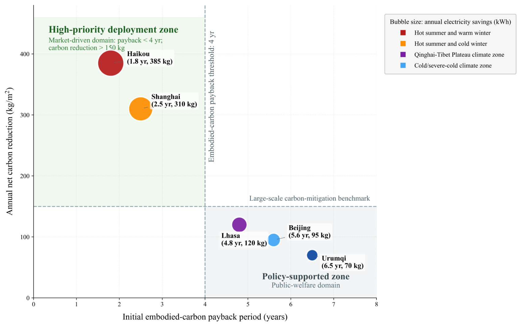
Because the selected Lhasa CV-TOPSIS compromise solution has non-positive annual electricity saving, its CPP is not achieved and it is treated separately from the finite-payback cases.

As shown in Figure 8, carbon reduction benefits are not proportional to electricity savings alone because grid carbon factors vary across regions. Haikou is cooling-dominated and achieves the largest electricity saving, resulting in a CPP of 1.8 years. Beijing and Urumqi achieve smaller electricity savings because additional shading may reduce useful winter solar gains and increase heating demand. However, their higher grid carbon emission factors, 0.565 and 0.602 kg CO₂e/kWh, respectively, increase the carbon benefit per unit of saved electricity and keep their CPPs at 4.8 and 6.5 years. Shanghai shows a short CPP of 2.5 years because of its moderate embodied carbon burden and positive annual electricity saving. In contrast, the selected Lhasa compromise solution is not assigned a finite CPP because it increases annual energy use within the defined boundary.

4.4. Sensitivity of Carbon Payback Results

To examine the sensitivity of CPP to deterministic input assumptions, a bounding sensitivity analysis was conducted for the selected trade-off solutions. The three key parameters determining CPP—annual electricity saving ($\Delta E$), grid carbon emission factor ($E{F}_{\mathrm{grid}}$), and upfront embodied carbon ($E{C}_{\mathrm{upfront}}$)—were varied by $\pm 20\%$ to bracket plausible uncertainty in material-carbon data, operational savings, and future grid carbon factors.

Because these parameters jointly affect the net carbon flow, combined extreme-case scenarios were evaluated. Under the conservative condition (+20% embodied carbon, −20% energy saving, and −20% grid emission factor), CPP increases to 1.875 times the baseline value. Conversely, under the optimistic condition (−20% embodied carbon, +20% energy saving, and +20% grid emission factor), CPP decreases to approximately 0.556 times the baseline value.

As shown in

Table 9. Carbon payback sensitivity bounds under material-carbon and grid-factor variations.

Typical City	Baseline CPP (${\mathit{CPP}}_0$)	Optimistic CPP	Conservative CPP
Haikou	1.8 years	1.0 years	3.4 years
Shanghai	2.5 years	1.4 years	4.7 years
Beijing	4.8 years	2.7 years	9.0 years
Urumqi	6.5 years	3.6 years	12.2 years
Lhasa	N.A.	N.A.	N.A.

Note: N.A. = not achieved because $\Delta E\le 0$.

, the sensitivity bounds indicate that Haikou and Shanghai remain highly carbon-effective even under the worst-case scenario, with their maximum CPPs extending to only 3.4 and 4.7 years, respectively. In contrast, Beijing and Urumqi are more sensitive to uncertainty; their conservative CPPs extend to 9.0 and 12.2 years, which begin to approach the typical lifespan of external shading components. The selected Lhasa compromise solution remains carbon-ineffective regardless of parameter variations, as its annual energy saving is fundamentally non-positive. This bounding check indicates that while absolute payback years may fluctuate, the relative feasibility ranking of the selected passive shading retrofits remains broadly unchanged under the assumed uncertainty range.

The $\pm 20\%$ perturbation of annual electricity savings is used here as a bounding proxy for the residual uncertainty of the reduced-order thermal model. It should not be interpreted as a full probabilistic propagation of the reported CV(RMSE) through the Pareto optimization and CV-TOPSIS decision process.

4.5. Practical Implications and Exploratory Stock-Scale Scenario

For practical retrofit design, the key implication is that passive shading should be differentiated by both climate conditions and grid carbon intensity. Cooling-dominated regions can benefit from deeper external shading and lower SHGC glazing. Mixed climates require a more balanced combination of shading depth and SHGC, because summer solar rejection must not eliminate useful winter gains. In heating-dominated regions, fixed shading should be applied conservatively because excessive solar blocking may increase winter heating demand.

For high-altitude, heating-dominated cities such as Lhasa, fixed shading should be applied cautiously, and movable or sensor-controlled shading should be considered as an alternative subject to additional cost, maintenance, control-energy, and embodied carbon assessment [10,11].

These implications are generalizable mainly as climate-adaptive design tendencies, not as direct stock-scale predictions. In real retrofit planning, the absolute energy savings, CPP values, and selected geometries should be recalibrated with local residential archetypes, envelope conditions, occupancy behavior, HVAC operation, and monitored energy use data.

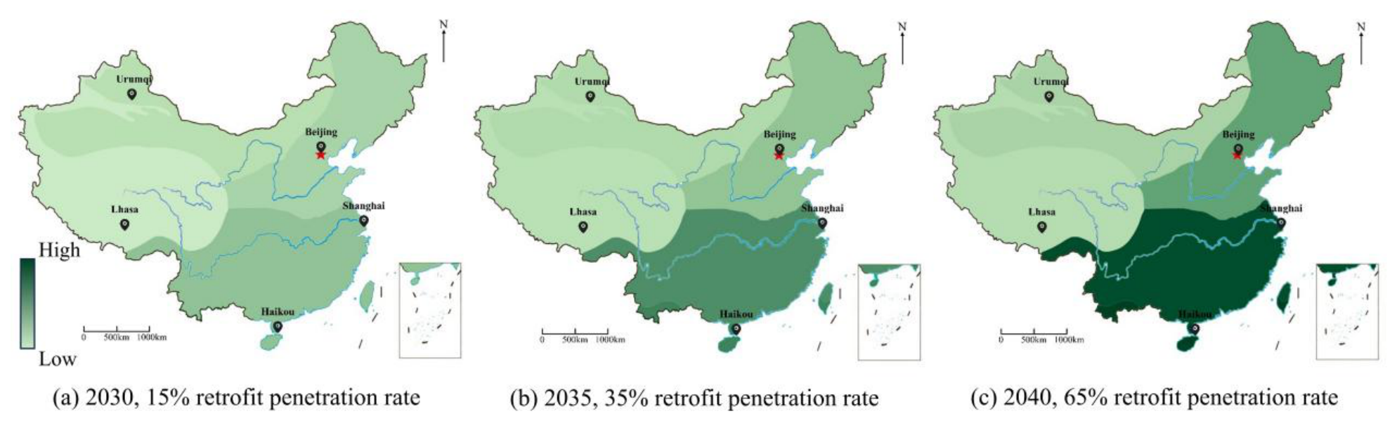
The national-scale exercise is retained only as an exploratory illustration of how climate-dependent payback tendencies may affect staged retrofit deployment. Because it extrapolates representative city results using simplified retrofit penetration assumptions and static grid emission factors, the results should be interpreted as order-of-magnitude policy signals rather than validated province-level forecasts. Future grid decarbonization would reduce the carbon benefit per unit of electricity saved and may lengthen CPP; practical planning should therefore use scenario-based or dynamic grid emission factors.

Figure 9 illustrates the cumulative net carbon reduction under the assumed staged penetration scenario.

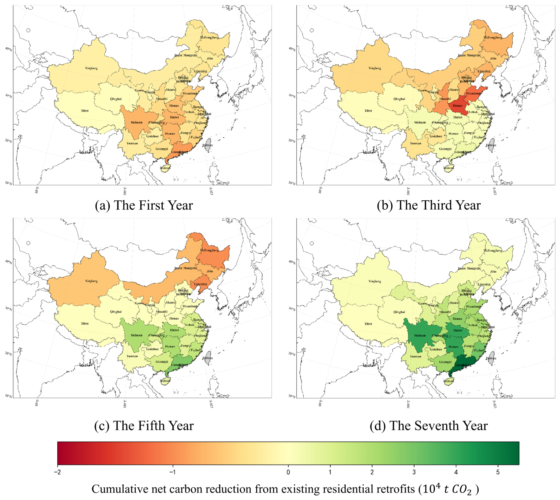
Figure 10 shows the spatial distribution of cumulative net carbon reduction under the same scenario. Cooling-dominated southern regions tend to reach positive net carbon reduction earlier, whereas northern, northwestern, and high-altitude regions show slower recovery because fixed shading provides smaller annual savings and may reduce useful winter solar gains. These exploratory patterns suggest stronger carbon payback potential in cooling-dominated regions, but they should not be interpreted as validated stock-scale predictions. Province-level residential stock data, monitored energy use data, dynamic grid carbon factors, and cost data are required before these estimates can support detailed retrofit planning.

4.6. Limitations

Several limitations define the appropriate use of the proposed method. First, UPDEM uses a reduced-order 2R2C thermal model benchmarked against EnergyPlus reference loads rather than calibrated with monitored data from the selected Chinese residential buildings; the energy-saving values are therefore comparative estimates under consistent assumptions, not measured outcomes. A full probabilistic propagation of modeling uncertainties through the Pareto optimization and CV-TOPSIS decision process remains future work. Second, occupant behavior is represented deterministically. Constant HVAC set points and a constant equivalent internal heat gain were used to maintain comparability across climates; in real buildings, thermostat preferences, intermittent air-conditioning use, window opening, and occupancy schedules can substantially alter energy savings, Pareto rankings, and CPP [60]. Third, the visual-related objective is represented by a transmitted solar exposure proxy rather than illuminance- or luminance-based metrics such as UDI, DGI, DGP, sDA, or ASE; the 15 and 250 W/m² thresholds are internal radiometric screening thresholds and should not be interpreted as human visual comfort criteria. Fourth, the design space is limited to fixed passive shading geometries. Movable or dynamically controlled shading systems are not included, although they may be more suitable in high-altitude, heating-dominated regions; future work should extend the decision variables to include control schedules, actuator energy, and embodied carbon of dynamic systems [10,11]. Fifth, the carbon assessment covers A1–A4 and B6 only. Excluded stages would systematically shift absolute CPP values but are unlikely to alter the relative cross-climate feasibility rankings because the boundary is applied consistently. Sixth, no structural capacity assessment was performed. If reinforcement, special anchorage, or wall repairs are required, their costs and embodied carbon should be included in project-specific LCA, and CPP values would be longer than reported here [54,55]. Seventh, the case study is based on a single 80 m² prototype and static grid carbon factors; transfer to other stocks requires local archetypes, envelope data, occupancy and HVAC schedules, dynamic grid factors, and preferably monitored validation. For these reasons, the framework should be regarded as a screening-level comparative method for early retrofit assessment, not as a direct stock-scale prediction tool.

5. Conclusions

This study developed a screening-level multi-objective method for climate-adaptive passive shading retrofits of existing residential buildings. The method integrates hourly solar–shading evaluation, a reduced-order 2R2C thermal model, NSGA-II optimization, CV-TOPSIS decision-making, and life-cycle-informed carbon payback assessment within an A1–A4 + B6 boundary.

The results show that the selected retrofit morphology varies strongly with climate. Cooling-dominated Haikou favors lower SHGC values and deeper east–west shading, achieving the largest annual electricity saving of 2030.3 kWh/yr and the shortest CPP of 1.8 years. Shanghai requires a more balanced solution, whereas Beijing and Urumqi favor higher SHGC values and constrained south-facing fixed overhangs to preserve winter solar gains. Ultimately, the carbon effectiveness of a retrofit strategy is governed not only by operational energy savings but also by the upfront embodied carbon and the specific regional grid carbon intensity. In Lhasa, the selected CV-TOPSIS compromise solution reduces the transmitted solar exposure proxy but increases annual energy use by 706.1 kWh/yr, indicating that this selected compromise is not carbon-effective within the defined assessment boundary. This finding should not be generalized to all possible shading alternatives; movable or dynamically controlled shading should be examined in future work for such high-altitude, heating-dominated contexts.

The proposed method is suitable for comparative early-stage screening of climate-specific retrofit alternatives rather than for direct prediction of measured stock-scale performance. Future work should incorporate monitored residential data, standard daylight and glare metrics, dynamic grid carbon factors, cost data, and probabilistic uncertainty analysis before broader planning application.

References

1. United Nations Environment Programme; Global Alliance for Buildings and Construction. Global Status Report for Buildings and Construction 2024/2025; UNEP: Nairobi, Kenya, 2025. [Google Scholar]
2. IPCC. Climate Change 2022: Mitigation of Climate Change. Contribution of Working Group III to the Sixth Assessment Report of the Intergovernmental Panel on Climate Change; Cambridge University Press: Cambridge, UK, 2022. [Google Scholar]
3. Ministry of Housing and Urban-Rural Development of the People’s Republic of China; National Development and Reform Commission. Implementation Plan for Carbon Peaking in Urban and Rural Construction; Ministry of Housing and Urban-Rural Development of the People’s Republic of China: Beijing, China; National Development and Reform Commission: Beijing, China, 2022.
4. GB/T 51366–2019; Standard for Building Carbon Emission Calculation. China Architecture & Building Press: Beijing, China, 2019.
5. GB 50176–2016; Code for Thermal Design of Civil Buildings. China Architecture & Building Press: Beijing, China, 2016.
6. Loonen, R.C.G.M.; Trčka, M.; Cóstola, D.; Hensen, J.L.M. Climate adaptive building shells: State-of-the-art and future challenges. Renew. Sustain. Energy Rev. 2013, 25, 483–493. [Google Scholar] [CrossRef]
7. Wu, H.; Zhang, T. Multi-objective optimization of energy, visual, and thermal performance for building envelopes in China’s hot summer and cold winter climate zone. J. Build. Eng. 2022, 59, 105034. [Google Scholar] [CrossRef]
8. Tzempelikos, A.; Athienitis, A.K. The impact of shading design and control on building cooling and lighting demand. Sol. Energy 2007, 81, 369–382. [Google Scholar] [CrossRef]
9. Palmero-Marrero, A.I.; Oliveira, A.C. Effect of louver shading devices on building energy requirements. Appl. Energy 2010, 87, 2040–2049. [Google Scholar] [CrossRef]
10. Konstantoglou, M.; Tsangrassoulis, A. Dynamic operation of daylighting and shading systems: A literature review. Renew. Sustain. Energy Rev. 2016, 60, 268–283. [Google Scholar] [CrossRef]
11. Naderi, E.; Sajadi, B.; Behabadi, M.A.; Naderi, E. Multi-objective simulation-based optimization of controlled blind specifications to reduce energy consumption, and thermal and visual discomfort: Case studies in Iran. Build. Environ. 2020, 169, 106570. [Google Scholar] [CrossRef]
12. Nabil, A.; Mardaljevic, J. Useful daylight illuminance: A new paradigm for assessing daylight in buildings. Light. Res. Technol. 2005, 37, 41–59. [Google Scholar] [CrossRef]
13. Nabil, A.; Mardaljevic, J. Useful daylight illuminances: A replacement for daylight factors. Energy Build. 2006, 38, 905–913. [Google Scholar] [CrossRef]
14. Reinhart, C.F.; Mardaljevic, J.; Rogers, Z. Dynamic daylight performance metrics for sustainable building design. LEUKOS 2006, 3, 7–31. [Google Scholar] [CrossRef]
15. Wienold, J.; Christoffersen, J. Evaluation methods and development of a new glare prediction model for daylight environments with the use of CCD cameras. Energy Build. 2006, 38, 743–757. [Google Scholar] [CrossRef]
16. Evins, R. A review of computational optimization methods applied to sustainable building design. Renew. Sustain. Energy Rev. 2013, 22, 230–245. [Google Scholar] [CrossRef]
17. Nguyen, A.T.; Reiter, S.; Rigo, P. A review on simulation-based optimization methods applied to building performance analysis. Appl. Energy 2014, 113, 1043–1058. [Google Scholar] [CrossRef]
18. Machairas, V.; Tsangrassoulis, A.; Axarli, K. Algorithms for optimization of building design: A review. Renew. Sustain. Energy Rev. 2014, 31, 101–112. [Google Scholar] [CrossRef]
19. Asadi, E.; da Silva, M.G.; Antunes, C.H.; Dias, L. Multi-objective optimization for building retrofit strategies: A model and an application. Energy Build. 2012, 44, 81–87. [Google Scholar] [CrossRef]
20. Asadi, E.; da Silva, M.G.; Antunes, C.H.; Dias, L.; Glicksman, L. Multi-objective optimization for building retrofit: A model using genetic algorithm and artificial neural network and an application. Energy Build. 2014, 81, 444–456. [Google Scholar] [CrossRef]
21. Mendez Echenagucia, T.; Capozzoli, A.; Cascone, Y.; Sassone, M. The early design stage of a building envelope: Multi-objective search through heating, cooling and lighting energy performance analysis. Appl. Energy 2015, 154, 577–591. [Google Scholar] [CrossRef]
22. Delgarm, N.; Sajadi, B.; Kowsary, F.; Delgarm, S. Multi-objective optimization of the building energy performance: A simulation-based approach by means of particle swarm optimization. Appl. Energy 2016, 170, 293–303. [Google Scholar] [CrossRef]
23. Ascione, F.; Bianco, N.; De Masi, R.F.; Mauro, G.M.; Vanoli, G.P. Design of the building envelope: A novel multi-objective approach for the optimization of energy performance and thermal comfort. Sustainability 2015, 7, 10809–10836. [Google Scholar] [CrossRef]
24. Zhai, Y.; Wang, Y.; Huang, Y.; Meng, X. A multi-objective optimization methodology for window design considering energy consumption, thermal environment and visual performance. Renew. Energy 2019, 134, 1190–1199. [Google Scholar] [CrossRef]
25. Goia, F. Search for the optimal window-to-wall ratio in office buildings in different European climates and the implications on total energy saving potential. Sol. Energy 2016, 132, 467–492. [Google Scholar] [CrossRef]
26. Yu, J.; Yang, C.; Tian, L. Low-energy envelope design of residential building in hot summer and cold winter zone in China. Energy Build. 2008, 40, 1536–1546. [Google Scholar] [CrossRef]
27. Yu, J.; Tian, L.; Yang, C.; Xu, X.; Wang, J. Sensitivity analysis of energy performance for high-rise residential envelope in hot summer and cold winter zone of China. Energy Build. 2013, 64, 264–274. [Google Scholar] [CrossRef]
28. Cheung, C.K.; Fuller, R.J.; Luther, M.B. Energy-efficient envelope design for high-rise apartments. Energy Build. 2005, 37, 37–48. [Google Scholar] [CrossRef]
29. Lam, J.C.; Tsang, C.L.; Li, D.H.W.; Cheung, S.O. Residential building envelope heat gain and cooling energy requirements. Energy 2005, 30, 933–951. [Google Scholar] [CrossRef]
30. Huang, Y.; Niu, J.L.; Chung, T.M. Comprehensive analysis on thermal and daylighting performance of glazing and shading designs on office building envelope in cooling-dominant climates. Appl. Energy 2014, 134, 215–228. [Google Scholar] [CrossRef]
31. U.S. Department of Energy. EnergyPlus Engineering Reference; U.S. Department of Energy: Washington, DC, USA, 2024. Available online: https://energyplus.net/documentation (accessed on 1 June 2025).
32. Deb, K.; Pratap, A.; Agarwal, S.; Meyarivan, T. A fast and elitist multiobjective genetic algorithm: NSGA-II. IEEE Trans. Evol. Comput. 2002, 6, 182–197. [Google Scholar] [CrossRef]
33. Deb, K.; Agrawal, R.B. Simulated binary crossover for continuous search space. Complex Syst. 1995, 9, 115–148. [Google Scholar]
34. Deb, K. Multi-Objective Optimization Using Evolutionary Algorithms; John Wiley & Sons: Chichester, UK, 2001. [Google Scholar]
35. Fraisse, G.; Viardot, C.; Lafabrie, O.; Achard, G. Development of a simplified and accurate building model based on electrical analogy. Energy Build. 2002, 34, 1017–1031. [Google Scholar] [CrossRef]
36. Bacher, P.; Madsen, H. Identifying suitable models for the heat dynamics of buildings. Energy Build. 2011, 43, 1511–1522. [Google Scholar] [CrossRef]
37. Kramer, R.; van Schijndel, J.; Schellen, H. Simplified thermal and hygric building models: A literature review. Front. Archit. Res. 2012, 1, 318–325. [Google Scholar] [CrossRef]
38. Reynders, G.; Nuytten, T.; Saelens, D. Potential of structural thermal mass for demand-side management in dwellings. Build. Environ. 2013, 64, 187–199. [Google Scholar] [CrossRef]
39. Harish, V.S.K.V.; Kumar, A. A review on modeling and simulation of building energy systems. Renew. Sustain. Energy Rev. 2016, 56, 1272–1292. [Google Scholar] [CrossRef]
40. ISO 14040:2006; Environmental Management—Life Cycle Assessment—Principles and Framework. ISO: Geneva, Switzerland, 2006.
41. ISO 14044:2006; Environmental Management—Life Cycle Assessment—Requirements and Guidelines. ISO: Geneva, Switzerland, 2006.
42. EN 15978:2011; Sustainability of Construction Works—Assessment of Environmental Performance of Buildings—Calculation Method. CEN: Brussels, Belgium, 2011.
43. Cabeza, L.F.; Rincón, L.; Vilariño, V.; Pérez, G.; Castell, A. Life cycle assessment (LCA) and life cycle energy analysis (LCEA) of buildings and the building sector: A review. Renew. Sustain. Energy Rev. 2014, 29, 394–416. [Google Scholar] [CrossRef]
44. Ibn-Mohammed, T.; Greenough, R.; Taylor, S.; Ozawa-Meida, L.; Acquaye, A. Operational vs. embodied emissions in buildings—A review of current trends. Energy Build. 2013, 66, 232–245. [Google Scholar] [CrossRef]
45. Pomponi, F.; Moncaster, A. Embodied carbon mitigation and reduction in the built environment—What does the evidence say? J. Environ. Manag. 2016, 181, 687–700. [Google Scholar] [CrossRef] [PubMed]
46. Dixit, M.K.; Fernández-Solís, J.L.; Lavy, S.; Culp, C.H. Identification of parameters for embodied energy measurement: A literature review. Energy Build. 2010, 42, 1238–1247. [Google Scholar] [CrossRef]
47. Dixit, M.K.; Fernández-Solís, J.L.; Lavy, S.; Culp, C.H. Need for an embodied energy measurement protocol for buildings: A review paper. Renew. Sustain. Energy Rev. 2012, 16, 3730–3743. [Google Scholar] [CrossRef]
48. Saynajoki, A.; Heinonen, J.; Junnila, S. A scenario analysis of the life cycle greenhouse gas emissions of a new residential area. Environ. Res. Lett. 2012, 7, 034037. [Google Scholar] [CrossRef]
49. Hwang, C.L.; Yoon, K. Multiple Attribute Decision Making: Methods and Applications; Springer: Berlin, Germany, 1981. [Google Scholar] [CrossRef]
50. Opricovic, S.; Tzeng, G.H. Compromise solution by MCDM methods: A comparative analysis of VIKOR and TOPSIS. Eur. J. Oper. Res. 2004, 156, 445–455. [Google Scholar] [CrossRef]
51. Circular Ecology. Inventory of Carbon and Energy (ICE) Database. Available online: https://circularecology.com/embodied-carbon-footprint-database.html (accessed on 3 July 2026).
52. GB 50176–1993; Thermal Design Code for Civil Buildings. China Planning Press: Beijing, China, 1993.
53. GB 50736–2012; Design Code for Heating Ventilation and Air Conditioning of Civil Buildings. China Architecture & Building Press: Beijing, China, 2012.
54. GB 55021–2021; General Code for Assessment and Rehabilitation of Existing Buildings. China Architecture & Building Press: Beijing, China, 2021.
55. GB 50009–2012; Load Code for the Design of Building Structures. China Architecture & Building Press: Beijing, China, 2012.
56. Angizeh, F.; Ghofrani, A.; Jafari, M.A. Dataset on Hourly Load Profiles for a Set of 24 Facilities from Industrial, Commercial, and Residential End-use Sectors. Mendeley Data 2020. Version 1. [Google Scholar] [CrossRef]
57. Wang, S.; Xu, X. Simplified building model for transient thermal performance estimation using GA-based parameter identification. Int. J. Therm. Sci. 2006, 45, 419–432. [Google Scholar] [CrossRef]
58. ASHRAE. ASHRAE Guideline 14-2014: Measurement of Energy, Demand, and Water Savings; American Society of Heating, Refrigerating and Air-Conditioning Engineers: Atlanta, GA, USA, 2014. [Google Scholar]
59. Department of Climate Change, Ministry of Ecology and Environment of the People’s Republic of China. Notice on the Reporting and Verification of Greenhouse Gas Emissions for Enterprises in Certain Key Industries from 2023 to 2025; Guo Huan Gui Qi Hou [2023] No. 2; Ministry of Ecology and Environment: Beijing, China, 2023.
60. Delzendeh, E.; Wu, S.; Lee, A.; Zhou, Y. The impact of occupants’ behaviours on building energy analysis: A research review. Renew. Sustain. Energy Rev. 2017, 80, 1061–1071. [Google Scholar] [CrossRef]
Figure 1. Overall workflow of the UPDEM-based screening method for passive external shading retrofits.
Buildings 16 02716 g001
Figure 2. System boundary and calculation logic for the life-cycle-informed carbon payback assessment.
Buildings 16 02716 g002
Figure 3. Locations and climatic zoning of the five representative Chinese cities, adapted from the Thermal Design Code for Civil Buildings (GB 50176-1993) [52].
Buildings 16 02716 g003
Figure 4. Reference residential unit and facade retrofit configuration used in the simulation cases.
Buildings 16 02716 g004
Figure 5. Benchmark comparison between the reduced-order UPDEM thermal model and EnergyPlus reference loads.
Buildings 16 02716 g005
Figure 6. Pareto-front distributions obtained from NSGA-II optimization for the five representative cities.
Buildings 16 02716 g006
Figure 7. Facade section drawings of the selected CV-TOPSIS trade-off retrofit solutions.
Buildings 16 02716 g007
Figure 8. Multidimensional carbon reduction quadrant analysis for the selected retrofit solutions. The selected Lhasa compromise solution is treated as a non-payback case because its annual electricity saving is negative.
Buildings 16 02716 g008
Figure 9. Cumulative net carbon reduction under the exploratory staged retrofit penetration scenario. The red star denotes Beijing as the national capital on the base map.
Buildings 16 02716 g009
Figure 10. Spatial distribution of cumulative net carbon reduction under the exploratory staged scenario.
Buildings 16 02716 g010