Explainable Machine Learning Reveals Seasonal Dynamics of Heat Inequality and Cooling Efficiency Bias Across 15 Chinese Cities

Abstract

Urban heat inequality represents a critical barrier to inclusive climate-resilient governance. While existing research has extensively mapped surface temperature patterns, the dynamic evolution of human thermal stress and the divergent regulatory efficiencies of cooling features across socio-economic contexts remain poorly understood. This study integrates multi-source datasets from 15 typical Chinese cities, employing a machine learning framework and GeoShapley interpretation to resolve the drivers of heat inequality across spatio-temporal and mechanistic dimensions. The findings demonstrate that high-density urbanization in China leads to a spatial synchronization of wealth and heat exposure, contrasting with the “Luxury Effect” observed in low-density Western contexts and indicating that high-income urban cores bear significantly higher absolute thermal stress. This inequality exhibits pronounced seasonal dynamics, where extreme summer conditions non-linearly amplify exposure gaps between socio-economic groups. Crucially, the results identify a systemic failure of cooling mechanisms in low-income communities, where the empirical thermal response of physical features deviates from expected patterns, failing to mitigate or even exacerbating perceived heat stress. These results emphasize that urban mitigation should move beyond quantitative resource expansion toward efficiency restoration, utilizing targeted spatial optimization to achieve precision climate justice.

1. Introduction

Extreme heat events driven by climate change present a significant challenge to urban sustainability, with direct implications for the health of urban populations [1,2]. As urbanization increasingly focuses on the optimization of existing built environments, urban heat risk research is evolving from purely physical assessments to addressing complex issues of social equity [3,4,5]. Within the context of climate change, urban heat stress has transitioned from a meteorological phenomenon to a critical public health concern. The uneven distribution of heat exposure risks now stands as a major barrier to the development of inclusive and resilient cities.

In this context, the concept of “heat inequality” highlights the close correlation between intra-urban thermal risk distribution and socio-economic gradients [6,7]. In high-density urban areas, disparities in socio-economic status (SES) often result in unequal environmental exposure, leading to diverging levels of vulnerability across different social groups. This stratified exposure forces disadvantaged populations to bear a disproportionate share of environmental risks, thereby exacerbating urban inequities [8]. Consequently, a systematic analysis of the patterns and driving mechanisms of heat inequality is essential for understanding microclimate dynamics and supporting the pursuit of climate justice and resilient urban development.

Previous studies have extensively explored the correlation between urban economic levels and the thermal environment. The “Luxury Effect” theory posits that high-income neighborhoods typically benefit from superior cooling resources, such as higher green cover, which reduces their heat exposure risks [9,10,11]. However, this association exhibits significant seasonal fluctuations. Empirical evidence indicates that the intensity of heat inequality shifts with changes in background climate [12]. During peak temperature months, the explanatory power of socio-economic factors regarding heat exposure often undergoes a non-linear increase [13], leading to a rapid expansion of environmental risks for vulnerable populations.

Despite the growing focus on seasonal dynamics, most research continues to rely on satellite-derived Land Surface Temperature (LST) as the primary metric [14,15,16]. Although LST offers high accessibility, its inability to account for humidity, wind speed, and mean radiant temperature leads to significant biases in assessing socio-environmental justice. Given that shading and ventilation vary substantially across different socio-economic strata, LST often masks the extreme physiological heat stress experienced by disadvantaged groups. In contrast, the Universal Thermal Climate Index (UTCI) integrates multi-dimensional meteorological parameters, providing a more accurate reflection of physiological stress within complex urban environments [17,18]. Therefore, a high-resolution, long-term UTCI assessment framework is essential for identifying the mechanisms of heat inequality and supporting the environmental health of marginalized communities.

Urban microclimates are influenced by three-dimensional (3D) morphology, including building density, height, and vegetation structure [19]. These physical parameters are key factors in regulating environmental heat distribution and are linked to the spatial patterns of heat inequality [20,21]. When 3D morphology interacts with socio-economic gradients, the configuration of the physical environment affects the extent of heat exposure across different economic strata [22,23], collectively determining the spatial distribution of urban heat risk.

While the cooling effects of physical elements are well-documented, their moderating role in the relationship between wealth and heat exposure is complex. Empirical studies show that the cooling efficiency of 3D morphology exhibits spatial non-stationarity [21,24] and is affected by regional climate conditions, such as temperature and humidity [25,26]. However, existing research often treats socio-economic factors and background climate as independent variables, with few studies analyzing their joint influence on the marginal regulatory efficiency of physical elements within a unified framework.

This uncertainty makes it difficult to distinguish the drivers of heat inequality: whether the disparity stems from the uneven spatial allocation of cooling resources or from variations in the efficiency of physical elements under specific socio-climatic conditions. Therefore, analyzing the impact pathways of multi-dimensional features on heat exposure is essential for shifting the focus from simple resource provision to the optimization of mitigation efficiency.

With the advancement of urban big data and computing power, machine learning has been widely adopted to simulate complex urban microclimates and their socio-economic impacts due to its ability to capture non-linear relationships. In the field of heat inequality, algorithms such as Random Forest and XGBoost have proven effective in modeling the high-dimensional interactions between physical morphology, socio-economic status, and perceived thermal stress [27,28,29]. However, the “black-box” nature of these models can limit their utility in policy-making. To address this, interpretability frameworks like SHAP (Shapley Additive Explanations) have been introduced to decompose global predictions into individual feature contributions, identifying the relative importance of different drivers [30,31,32].

While SHAP is effective for global feature attribution, it often overlooks the spatial non-stationarity inherent in geographic data, making it difficult to analyze the local dynamics of heat inequality. The GeoShapley algorithm provides a framework to address this limitation [33]. GeoShapley enables the spatial decomposition of model predictions, allowing for the quantification of local contributions from factors such as GDP to heat stress variations, while capturing spatial heterogeneity [34,35,36]. This transition from global fitting to local spatial attribution provides a robust approach for analyzing how socio-economic gradients interact with the physical environment to influence heat inequality.

To address existing gaps in evaluation metrics and attribution methods, this study integrates 1 km resolution UTCI data, 3D urban morphology parameters, and socio-economic datasets for 15 Chinese cities. The objective is to analyze the joint influence of physical and socio-economic factors on urban heat exposure across different seasons.

The main contributions are:

(1) Transition from LST to perceived heat stress: Instead of relying on single-temporal LST, this study uses monthly UTCI to capture the actual physiological heat stress experienced by residents and its seasonal variations.

(2) Analysis of cooling performance across economic levels: This study identifies how the cooling effects of physical urban features vary with neighborhood income levels. These findings provide evidence for developing location-specific heat mitigation strategies.

(3) Application of GeoShapley for spatial attribution: By combining machine learning with the GeoShapley framework, this study quantifies the spatial contribution of socio-economic factors to heat stress. This approach addresses the “black-box” limitation of ML models and provides a clearer understanding of the drivers of heat inequality.

2. Methods

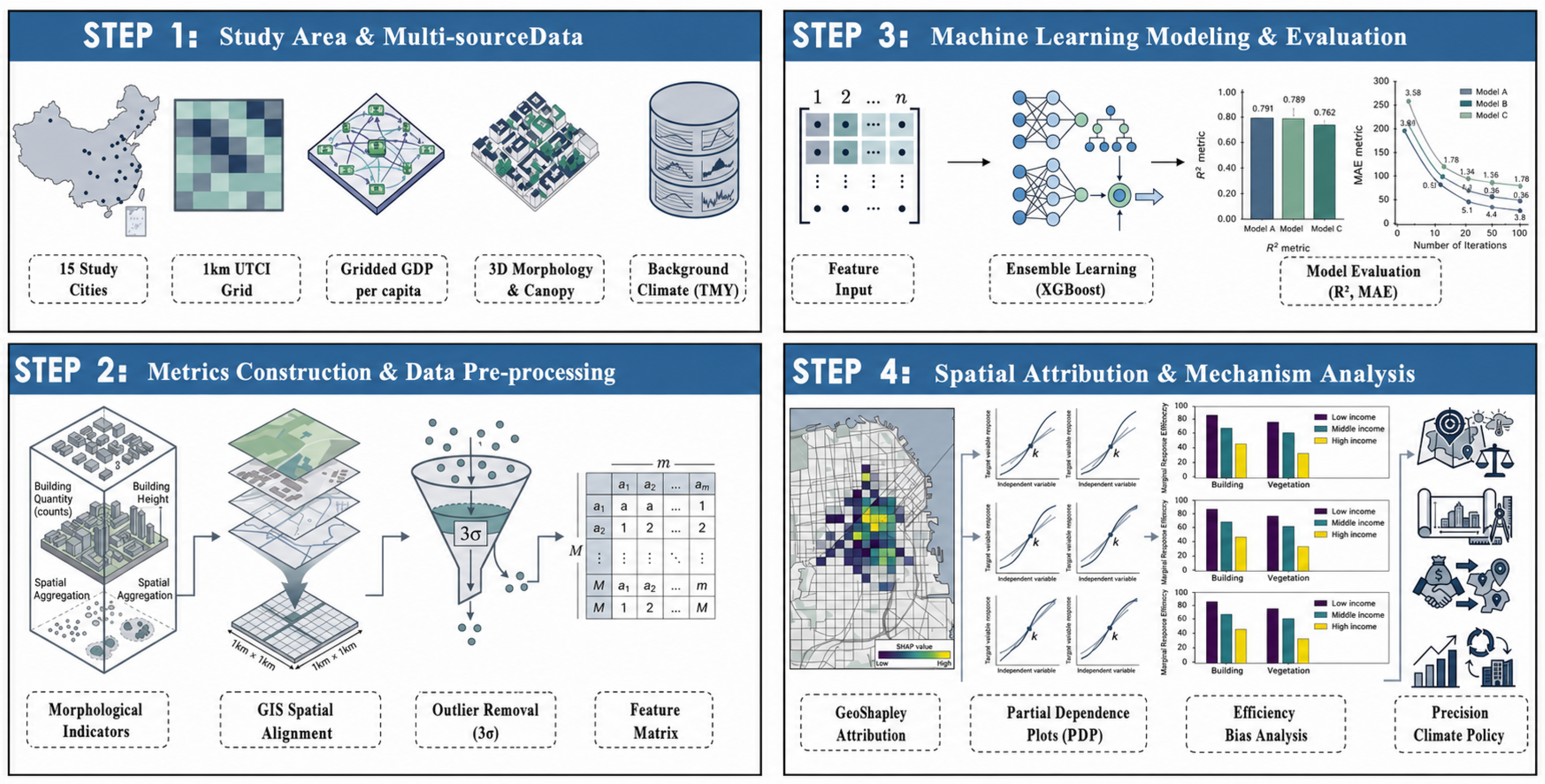
To systematically investigate the mechanisms driving urban heat inequality and the varying cooling efficiencies across socio-economic gradients, this study developed a comprehensive, data-driven analytical framework. As illustrated in Figure 1, the research workflow is structured into four interconnected phases. First, a multi-source data acquisition strategy was implemented across 15 representative Chinese cities (

Table A1. Summary of the 15 study cities and their characteristics.

City	Climate Zone	Grid Cells	Urban Characteristics
Guangzhou	Hot Summer & Warm Winter	10,401	Coastal megacity in South China
Suzhou	Hot Summer & Cold Winter	5629	Core city in the Yangtze River Delta
Beijing	Cold	4317	National capital on the North China Plain
Shanghai	Hot Summer & Cold Winter	3849	Coastal global financial center
Tianjin	Cold	2007	Major port city in North China
Zhengzhou	Cold	1853	Central inland transportation hub
Chengdu	Hot Summer & Cold Winter	1465	Major basin city in Southwest China
Xi’an	Cold	1355	Inland historical center in Northwest China
Shenyang	Severe Cold	1226	Regional hub in Northeast China
Qingdao	Cold	976	Coastal city on the Jiaodong Peninsula
Hefei	Hot Summer & Cold Winter	908	Inland city in East China
Nanjing	Hot Summer & Cold Winter	899	Core city in the Yangtze River Delta
Kunming	Mild	710	Plateau city in Southwest China
Nanning	Hot Summer & Warm Winter	526	Frontier city in South China
Harbin	Severe Cold	507	High-latitude city in Northeast China

) to integrate human thermal stress (UTCI), socio-economic levels (gridded GDP), 3D urban morphology, and background climate data. Second, a comprehensive morphological indicator system was constructed and rigorously pre-processed through GIS spatial alignment and outlier removal to generate a robust feature matrix. Third, an ensemble machine learning approach, optimized via the XGBoost algorithm, was employed to capture the complex, non-linear interactions among these microclimatic and socio-economic variables. Finally, explainable AI techniques—specifically the GeoShapley framework and Partial Dependence Plots (PDP)—were utilized to conduct fine-grained spatial attribution and extract the marginal response efficiency (slope k) of physical features across different income strata, ultimately informing precision climate policy.

2.1. Study Area and Data Sources

This study selects 15 representative Chinese cities covering diverse climatic zones, from cold regions in the north to monsoon climates in the south. These cities, characterized by high-intensity development and population density, provide a representative sample for analyzing the relationship between socio-economic gradients and urban microenvironments. To ensure spatio-temporal consistency across physical morphology, socio-economic indicators, and thermal parameters, 2020 is used as the baseline year.

A multi-source, high-resolution data framework was developed for quantitative analysis. The target variable is the Universal Thermal Climate Index (UTCI), obtained from the GloUTCI-M monthly 1 km dataset [37], which accounts for the combined effects of air temperature, humidity, wind speed, and mean radiant temperature. UTCI values are contextualized using standard thermal stress categories (e.g., 32–38 °C as ‘strong heat stress’) to provide a baseline for absolute risk assessment [18]. The GloUTCI-M dataset has been rigorously validated against meteorological station observations, ensuring its high reliability for urban-scale thermal assessment. Socio-economic status is represented by 1 km resolution downscaled GDP per capita (PPP) grid data [38]. This dataset ensures high spatial accuracy by harmonizing multi-level sub-national observations and employing an ensemble learning framework to capture fine-grained intra-urban economic heterogeneity. Physical environment parameters were extracted from the 3D-GloBFP 3D building footprint dataset [39] and the 1 m Global Canopy Height dataset [40] to quantify the 3D characteristics of buildings and vegetation. Additionally, Typical Meteorological Year (TMY) data from Climate. OneBuilding—including air temperature, humidity, and wind speed—were incorporated to control for the effects of background climate forcing on intra-urban heat exposure variations. TMY data was selected to provide a representative climatological baseline, filtering out annual stochastic weather anomalies to better isolate the structural impact of urban morphology on thermal environments.

2.2. Metrics and Data Pre-Processing

This study develops a system of eight morphological indicators across two categories—Building and Vegetation—to analyze the impact of the urban microenvironment on human thermal stress. These metrics are classified into four dimensions: Quantity (2D), representing physical stock; Quality (3D), representing volume and shading potential; Vertical Configuration, characterizing spatial roughness; and Horizontal Configuration, describing spatial compactness.

Specifically, the Quantity dimension is represented by the Building Coverage Ratio (BCR) and Vegetation Coverage Ratio (VCR), calculated as the ratio of the projected area of buildings or vegetation to the total area of each 1 km grid cell. Quality is quantified by Mean Height. Vertical Configuration is measured using the Height Coefficient of Variation (Height CV) to reflect spatial heterogeneity, while Horizontal Configuration uses the Aggregation Index (AI) to quantify the spatial connectivity of physical elements. These indicators serve as input variables to evaluate the response efficiency (k value) of physical elements across different socio-economic groups.

To ensure statistical robustness, a standard spatial resampling and cleaning procedure was implemented. First, GDP data, morphological indicators, and meteorological parameters were aligned to a 1 km × 1 km analysis grid using geospatial processing in Python. All geospatial processing was conducted in Python 3.9.13 using GeoPandas version 1.0.1. During the pre-processing phase, grid cells with missing values were excluded, and outliers were removed based on the 3σ rule. Outliers are primarily non-physical boundary artifacts and low-temperature noise (see

Table A2. Comparison of outlier removal schemes across 15 cities.

City	1σ Outliers	1σ Rate	2σ Outliers	2σ Rate	3σ Outliers	3σ Rate
Guangzhou	1756	16.88%	772	7.42%	368	3.54%
Suzhou	1525	27.09%	402	7.14%	217	3.86%
Beijing	677	15.68%	284	6.58%	142	3.29%
Shanghai	308	8.00%	150	3.90%	105	2.73%
Tianjin	346	17.24%	139	6.93%	78	3.89%
Zhengzhou	998	53.86%	66	3.56%	1	0.05%
Chengdu	268	18.29%	97	6.62%	56	3.82%
Xi’an	295	21.77%	97	7.16%	43	3.17%
Shenyang	250	20.39%	97	7.91%	39	3.18%
Qingdao	178	18.24%	76	7.79%	28	2.87%
Hefei	341	37.56%	97	10.68%	0	0.00%
Nanjing	415	46.16%	0	0.00%	0	0.00%
Kunming	131	18.45%	47	6.62%	22	3.10%
Nanning	193	36.69%	50	9.51%	0	0.00%
Harbin	100	19.72%	36	7.10%	16	3.16%

for city-specific removal counts). The cleaned dataset was then integrated into a feature matrix for non-linear modeling.

2.3. Machine Learning Modeling and Performance Evaluation

To analyze the non-linear relationships between urban morphology, socio-economic factors, meteorological conditions, and UTCI, this study established a regression framework based on ensemble learning. A total of 13 independent variables were utilized, comprising eight urban morphological indicators, four meteorological parameters (Ta, Pa, GHI, and Va), and one socio-economic indicator (GDP) (see

Table A3. Summary of input predictors for the ensemble learning models.

Category	Predictor	Full Name	Unit
Socio-economic	GDP	GDP per capita	Yuan
Quantity (2D)	B_BCR	Building Coverage Ratio	%
	V_VCR	Vegetation Coverage Ratio	%
Quality (3D)	B_MeanH	Building Mean Height	m
	V_MeanH	Vegetation Mean Height	m
Vertical	B_CVH	Building Height Coefficient of Variation	-
	V_CVH	Vegetation Height Coefficient of Variation	-
Horizontal	B_AI	Building Aggregation Index	-
	V_AI	Vegetation Aggregation Index	-
Meteorology	TMY_Ta	Air Temperature	°C
	TMY_Pa	Air Pressure	hPa
	TMY_GHI	Global Horizontal Irradiation	W/m2
	TMY_Va	Wind Speed	m/s
Target	UTCI	Universal Thermal Climate Index	°C

). Six algorithms were compared: XGBoost (XGB), LightGBM (LGB), CatBoost (CB), Random Forest (RF), Extra Trees (ET), and AdaBoost (Ada).

Model performance was evaluated using the coefficient of determination (R²) and Mean Absolute Error (MAE) to assess fitting accuracy and generalization across different cities and seasons. All candidate models underwent cross-validation using the datasets from the 15 study cities. By comparing the error metrics and explanatory power of each algorithm, the optimal model was selected as the base for subsequent spatial attribution and Partial Dependence Plot (PDP) analysis.

2.4. Spatial Attribution and Response Mechanism Analysis

This study employs the GeoShapley framework to interpret the machine learning model by quantifying the local contributions of socio-economic (GDP) and physical morphological factors to human thermal stress. GeoShapley decomposes the predicted UTCI values at the grid level, identifying the independent contribution (SHAP value) of each factor across different cities and months. These SHAP values quantify the explanatory power of socio-economic gradients regarding thermal heterogeneity and identify the coupling relationship between wealth and heat exposure.

To further analyze the variation in physical regulatory efficiency across socio-economic levels, Partial Dependence Plots (PDP) were used to extract the marginal response slopes of morphological factors. Spatial units were categorized into low-, middle-, and high-income groups based on GDP levels, and PDP curves were generated for each group. The response efficiency, k, is defined as the derivative of the PDP curve within a specific interval, representing the marginal change in UTCI per unit increase in physical input (e.g., vegetation or building metrics). By comparing the polarity and magnitude of k values across different income groups, this study quantifies whether the cooling efficiency of physical elements varies systematically across socio-economic gradients and identifies the effective thresholds for physical regulation.

3. Results

3.1. Spatio-Temporal Evolution of Human Heat Stress Inequality

3.1.1. Positive Spatial Coupling Between Economic Level and Heat Stress

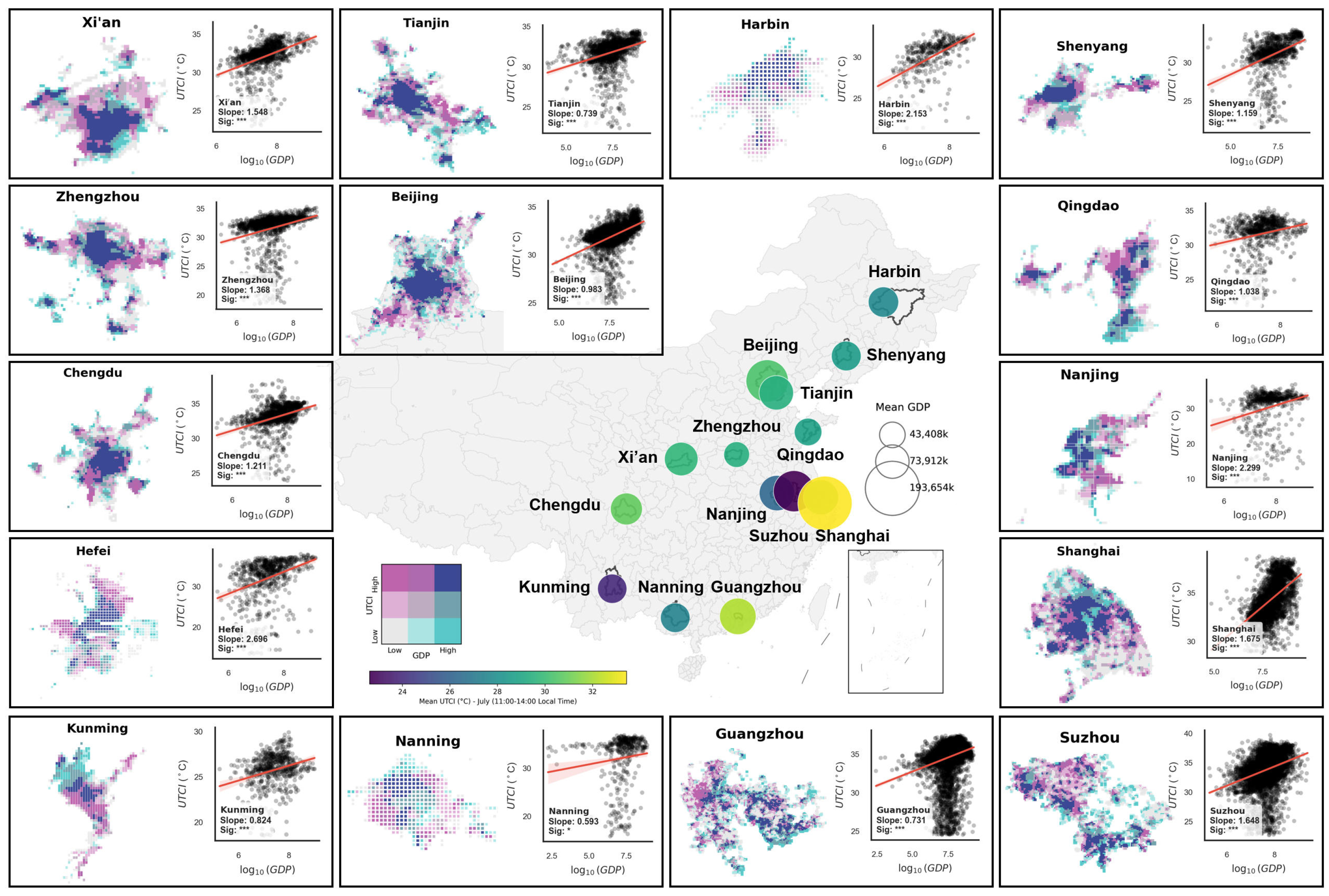
The study analyzed the spatial distribution of human thermal stress (UTCI) and economic levels (${\mathrm{l}\mathrm{o}\mathrm{g}}_{10}GDP$) during peak summer heat (July, 11:00–14:00) across 15 cities (Figure 2). The results indicate a high degree of spatial alignment between areas of intense thermal stress and high economic activity. This positive spatial coupling suggests that within the current urban development patterns of the studied cities, core economic zones—characterized by high impervious surface cover, building density, and anthropogenic heat emissions—are typically the most thermally stressed areas.

Statistical fitting shows that the regression slopes for all 15 cities are positive (Slope > 0) and statistically significant (p < 0.01), although sensitivity varies by city. Cities such as Hefei (2.696), Nanjing (2.289), and Harbin (2.153) exhibit high slope values, indicating that increases in economic intensity in these areas are associated with more pronounced environmental heat loads. In contrast, cities like Nanning (0.593) and Kunming (0.824) show considerably lower correlation strengths. These results quantify the significant heterogeneity in how different urban systems respond to economic intensification, providing a baseline for analyzing systemic biases in cooling efficiency.

3.1.2. Seasonal Fluctuations of Human Heat Stress Inequality

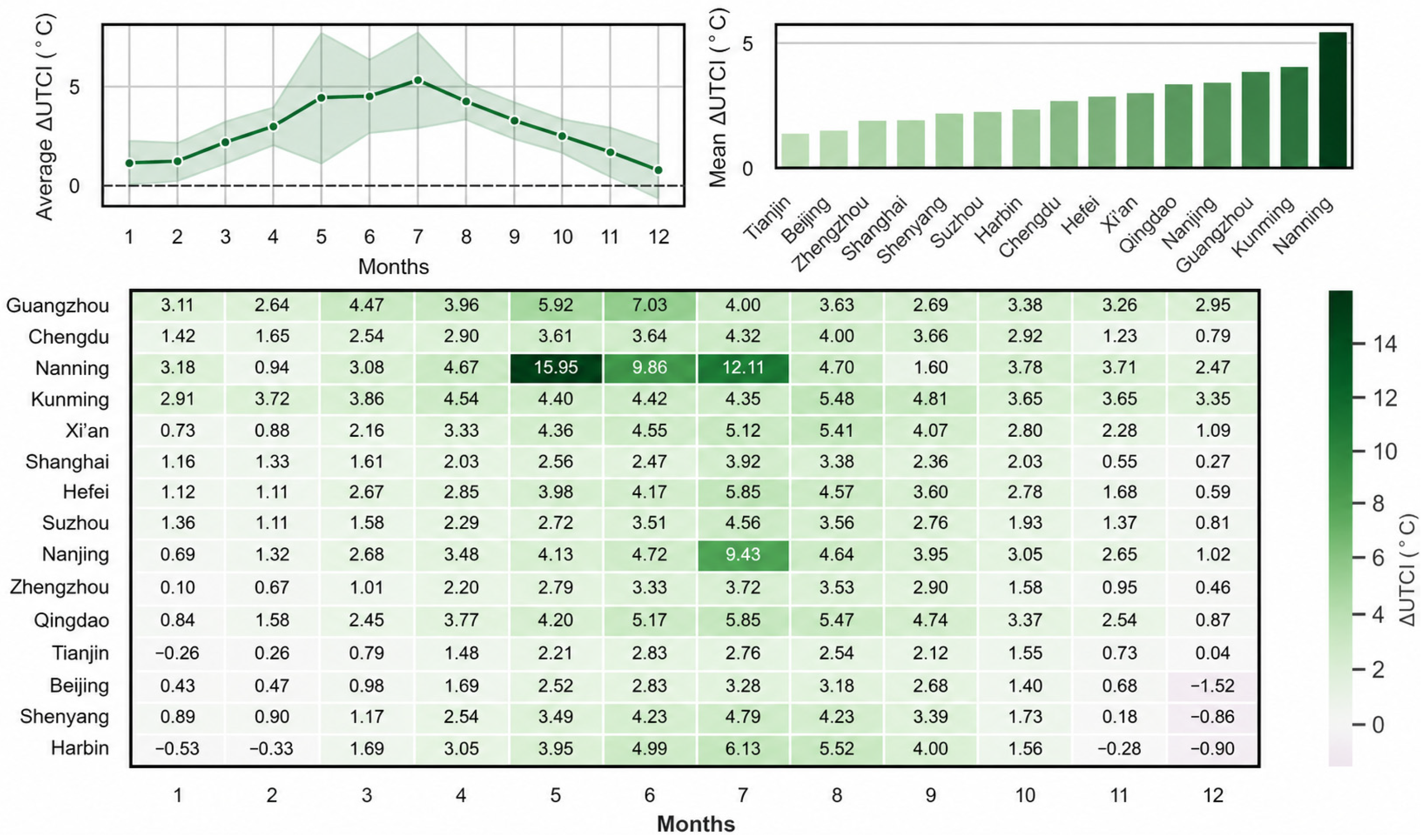
This study categorized 1 km grid cells into low-, middle-, and high-income groups using the tertile method. The average heat exposure disparity (∆UTCI)—defined as the difference in mean thermal stress between high- and low-income groups (${UTCI}_{High}-{UTCI}_{Low}$)—standardizes background temperature variations to quantify relative exposure differences derived from resource allocation. Results show that urban heat inequality in China exhibits seasonal fluctuations, with thermal stress disparities expanding as temperatures rise (Figure 3). In July, absolute UTCI levels across all cities exceeded the 32 °C ‘strong heat stress’ threshold, indicating that the observed exposure disparities (∆UTCI) occur within a high-risk thermal environment. The national average ∆UTCI peaks in July at over 5 °C, reflecting a substantial absolute exposure disparity where high-income groups experience higher thermal stress during extreme heat.

Heatmap analysis confirms substantial intensity variations across cities (Figure 3). For example, Nanning recorded a ∆UTCI of 15.95 °C in May, highlighting the impact of humid-hot climates on exposure disparities. Northern cities, such as Beijing and Harbin, exhibited negative disparities in December (e.g., −1.52 °C in Beijing), where high-income areas experienced lower thermal stress than low-income areas under extreme cold. These patterns confirm the moderating influence of macro-climatic backgrounds on the socio-spatial distribution of environmental risks.

3.1.3. Full-Cycle Robustness and Seasonal Polarity Reversal

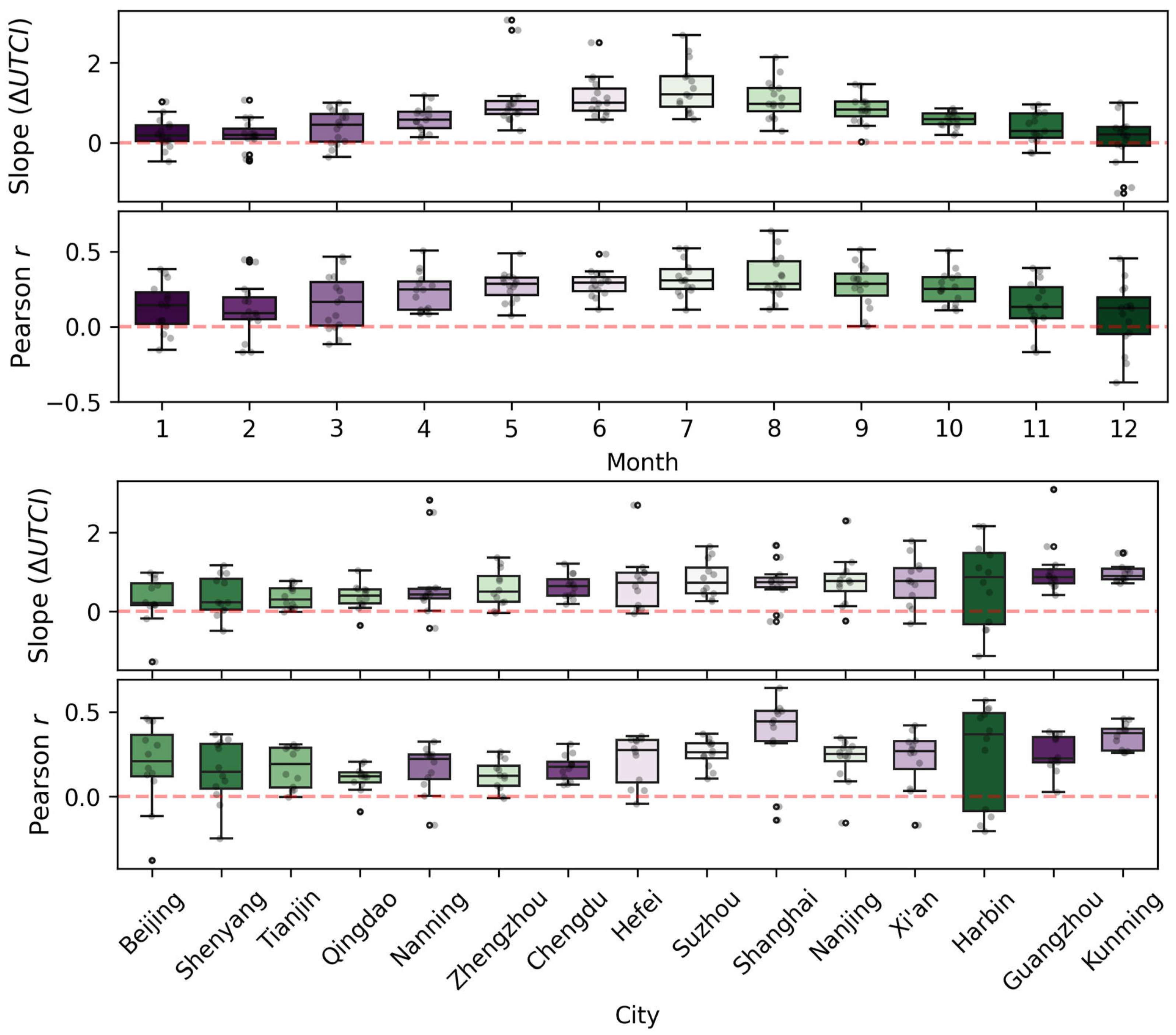
Full-sample regression analysis reveals a consistent association between wealth levels and thermal stress across the studied urban systems. Monthly statistics (Figure 4) indicate that both regression slopes and Pearson r coefficients exhibit strong seasonal synchronicity, with association strengths increasing alongside rising temperatures and peaking between July and August. At the city level, megacities such as Shanghai demonstrate high statistical stability, with median correlation coefficients near 0.45 and narrow fluctuation ranges. These patterns suggest that the influence of socio-economic status on spatial microclimates has become a structural characteristic in highly developed urban environments, representing a systemic rather than incidental phenomenon.

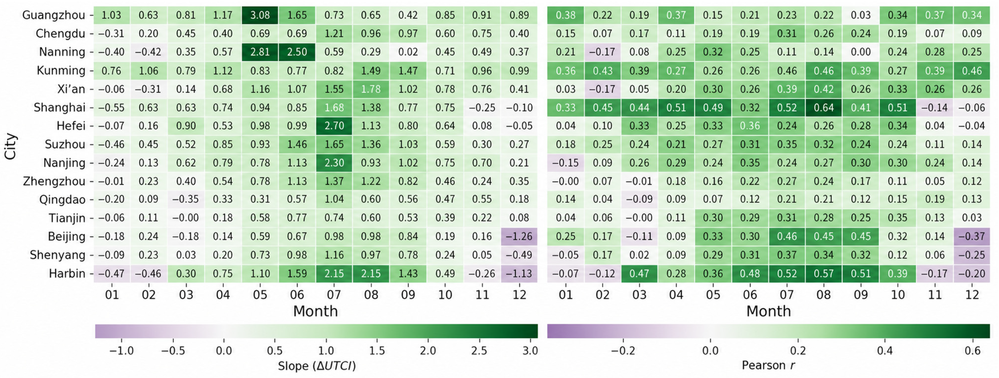
Monthly analysis via heatmap matrices (Figure 5) identifies regional variations in the timing of peak thermal inequality. Southern cities like Nanning and Guangzhou reach peak sensitivity between May and June, while inland cities such as Hefei and Nanjing experience maximum intensity in July. A notable reversal in association polarity occurs in northern cities during winter; Beijing, Shenyang, and Harbin exhibit negative slopes in December (e.g., −1.26 for Beijing and −1.13 for Harbin). This reversal, where high-income areas experience lower thermal stress (UTCI) than low-income areas under extreme cold, reflects a shift in how environmental contexts moderate the relationship between socio-economic status and thermal exposure.

3.2. Nonlinear Amplification of Heat Inequality by Background Environments

3.2.1. Moderating Effect of Background Climatic Factors

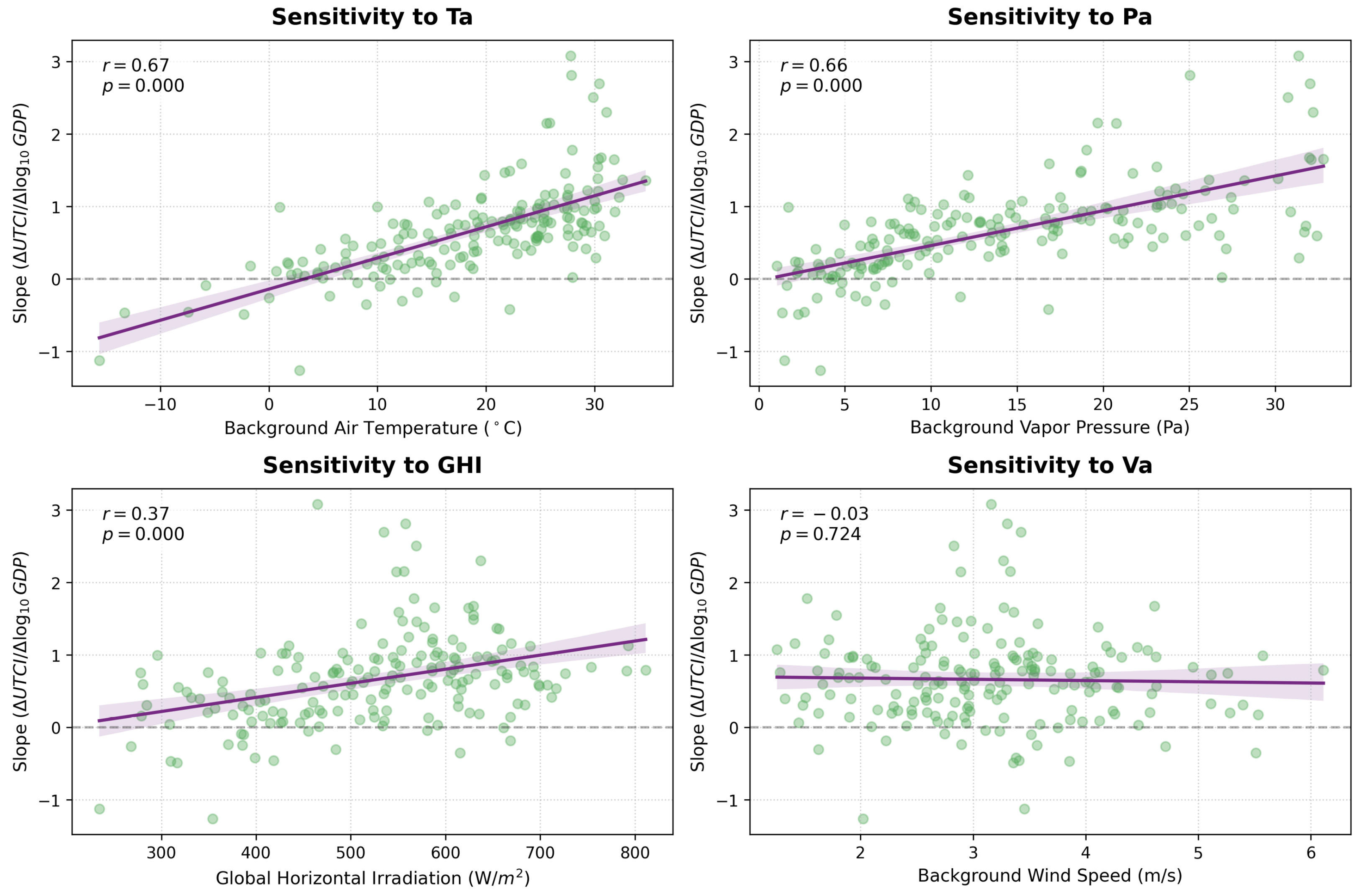
This study analyzed the sensitivity of heat inequality intensity (regression slope) to four background climatic factors (Figure 6). Results show that air temperature (Ta) and vapor pressure (Pa) are the primary variables influencing the intensity of heat inequality, with both exhibiting strong positive correlations with the slope (r = 0.67 and 0.66, respectively). This indicates that the distributive effect of socio-economic status on human heat stress intensifies under hotter and more humid conditions. In summer months or humid-hot southern cities, the heat exposure gap between different income communities widens as climatic forcing increases.

In addition to temperature and humidity, global horizontal irradiance (GHI) exhibits a positive moderating effect on heat inequality. This suggests that under high-radiation conditions, superior shading infrastructure in high-income areas—such as high-canopy greenery or shaded building designs—provides higher marginal cooling benefits, further increasing the exposure gap with low-income areas. In contrast, background wind speed (Va) shows no significant statistical association with the slope, indicating that wind speed does not systematically alter wealth-driven exposure disparities. Temperature and humidity are thus identified as the primary meteorological drivers of urban heat inequality.

3.2.2. Synergistic Amplification Effects of Environmental Factors

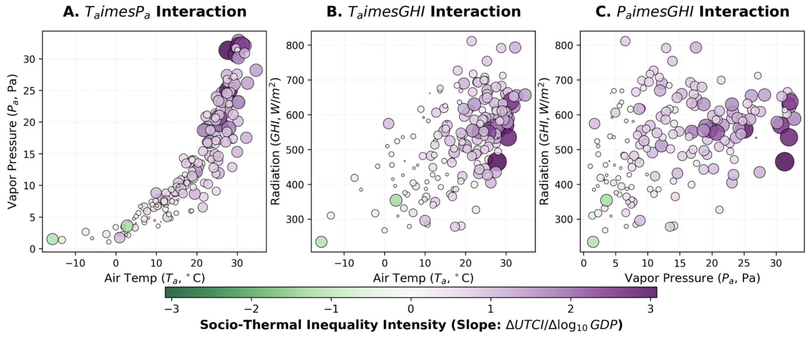
This section examines the synergistic regulation of thermal inequality intensity by various environmental factors (Figure 7). Results reveal a significant synergistic amplification effect between air temperature (Ta) and vapor pressure (Pa). When Ta > 25 °C and Pa > 15 Pa, the magnitude of the regression slope increases substantially. This indicates that heat inequality does not grow linearly with meteorological pressure but undergoes a non-linear escalation under hot and humid conditions, highlighting the role of environmental forcing in mediating social exposure risks.

Furthermore, the combined effect of global horizontal irradiance (GHI), temperature, and humidity further exacerbates the social exposure deficit. Under high-temperature conditions, intense radiation leads to a further increase in slope values, reflecting the amplified cooling benefits of physical infrastructure (e.g., shading) in high-income areas. In contrast, under dry-cold or low-temperature conditions, the interaction between these factors has a minimal impact on the slope. These non-linear characteristics provide a scientific basis for identifying critical thresholds of heat inequality and demonstrate that socio-economic disparities in thermal exposure are systematically amplified under extreme weather conditions.

3.3. Driver Identification and Seasonal Shifts in Feature Contribution

3.3.1. Performance Evaluation and Seasonal Stability of Machine Learning Models

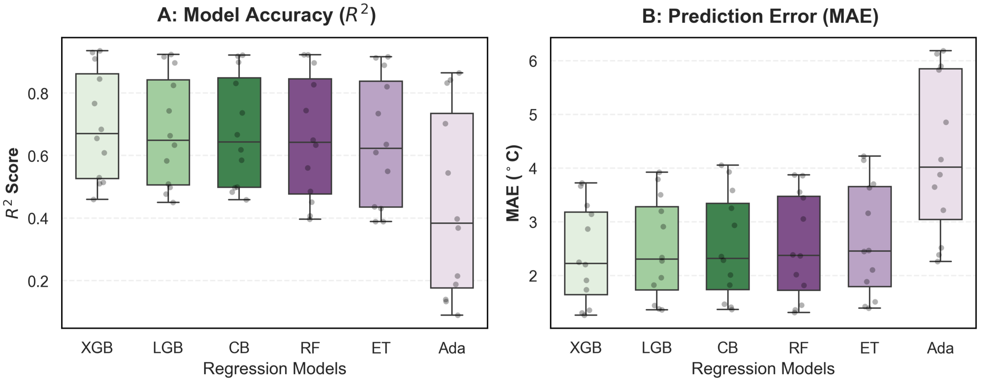
This study compared the performance of six machine learning algorithms in simulating UTCI. Benchmarking results (Figure 8) indicate that gradient boosting tree algorithms, specifically XGBoost (XGB) and LightGBM (LGB), outperformed other models in terms of explanatory power and predictive accuracy. The XGBoost model achieved a median R² of 0.65–0.70 and maintained a Mean Absolute Error (MAE) of approximately 2.2 °C. In contrast, AdaBoost was excluded due to its lower explanatory power (R² < 0.4) and high error volatility. Consequently, the optimized XGBoost model was selected as the base for further analysis.

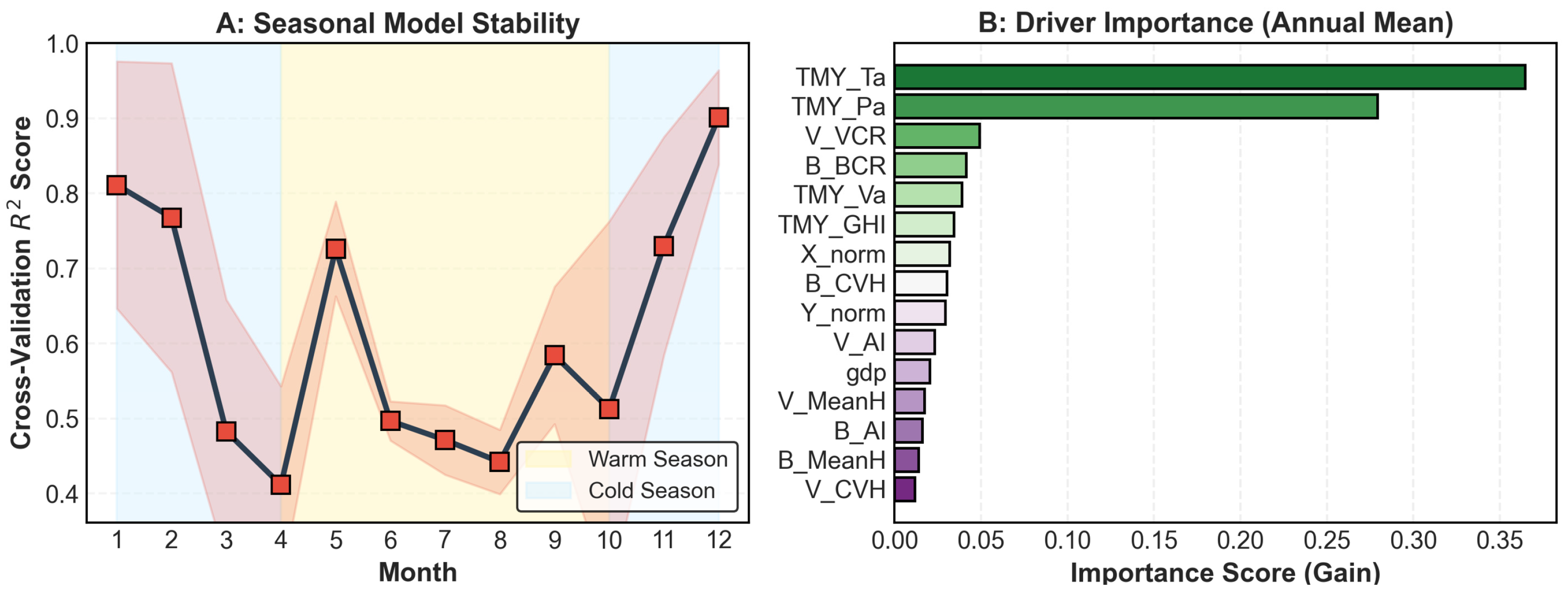
Further evaluation of the seasonal stability of the XGBoost model (Figure 9A) reveals distinct fluctuations in predictive performance. During winter (December to February), the model exhibits high explanatory power, with R² values ranging from 0.80 to 0.90. This suggests that under extreme cold conditions, human thermal stress is primarily governed by background meteorology and underlying surface characteristics. In summer, the R² decreases to approximately 0.45–0.50, likely due to the increased influence of microclimatic complexity and anthropogenic heat emissions. These seasonal variations in performance quantify the changing complexity of the urban thermal system under different environmental forcings and provide a reliable basis for identifying key drivers using GeoShapley. Comparative analyses with alternative machine learning architectures showed consistent seasonal performance patterns, suggesting that the lower R² in summer is an inherent property of increased microclimatic complexity rather than a model-specific limitation.

3.3.2. Global Feature Contributions and Seasonal Variations

Feature importance (Gain) analysis quantifies the annual contribution of each driver to urban thermal heterogeneity (Figure 9B). Background air temperature (Ta) and vapor pressure (Pa) are the primary contributors, with influence levels significantly exceeding those of urban physical elements. Among local regulators, vegetation coverage ratio (V_VCR) and building coverage ratio (B_BCR) exhibit the strongest influence. While the global contribution of GDP is moderate, its role in moderating socio-spatial exposure disparities is significant. This structure suggests a multi-level driving mechanism: background climate establishes the thermal baseline, urban morphology provides local regulation, and socio-economic factors influence the distribution of heat exposure across social strata.

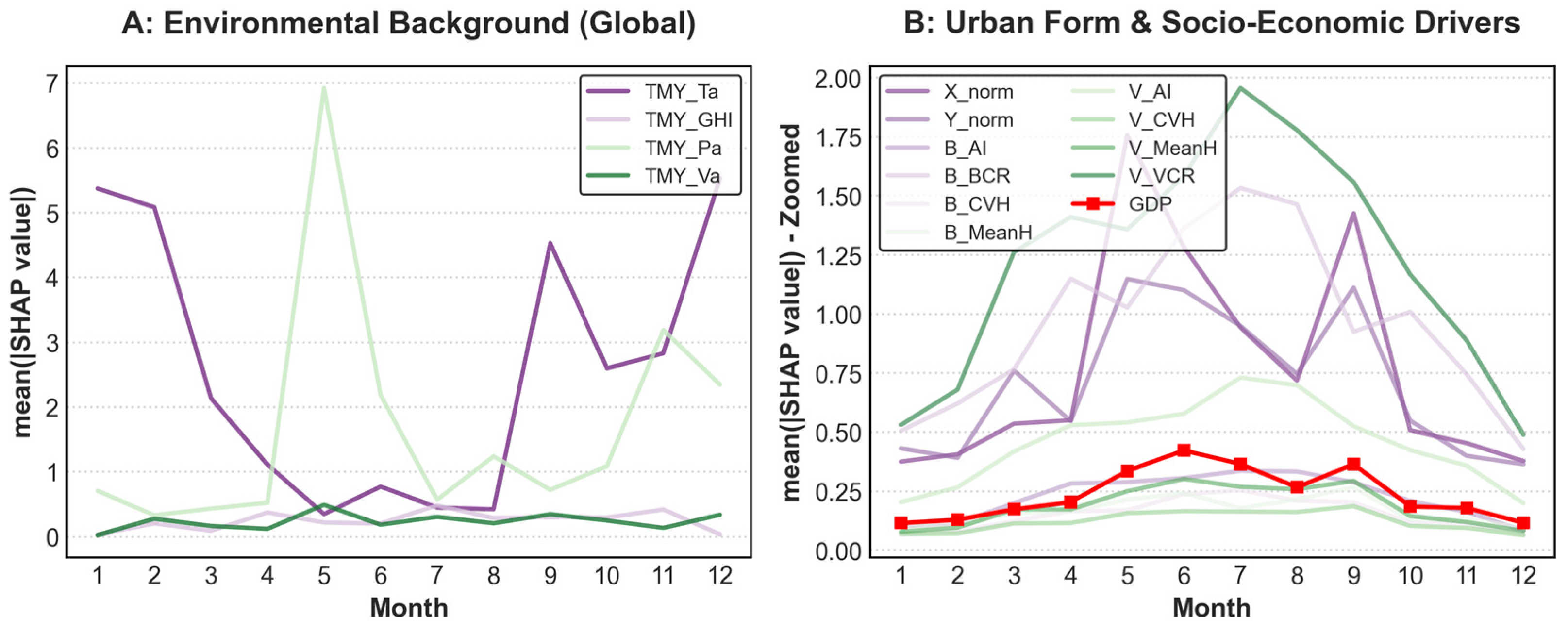
GeoShapley analysis reveals seasonal variations in these driving mechanisms (Figure 10). Regarding background factors, vapor pressure (Pa) peaks in importance in May, exceeding air temperature, which explains the early onset of heat inequality in southern cities. Among local physical factors, the regulatory weight of vegetation (V_VCR) reaches its maximum in July, serving as the primary cooling asset during peak summer. Notably, the contribution of GDP exhibits a seasonal pattern, with significant peaks in June and September as temperatures rise (Figure 10B). This increase in socio-economic influence indicates that heat inequality is systematically intensified under extreme thermal conditions.

3.4. Systematic Disparities in Resource Stocks and Cooling Efficiency

3.4.1. Disparities in the Spatial Allocation of Cooling Resources

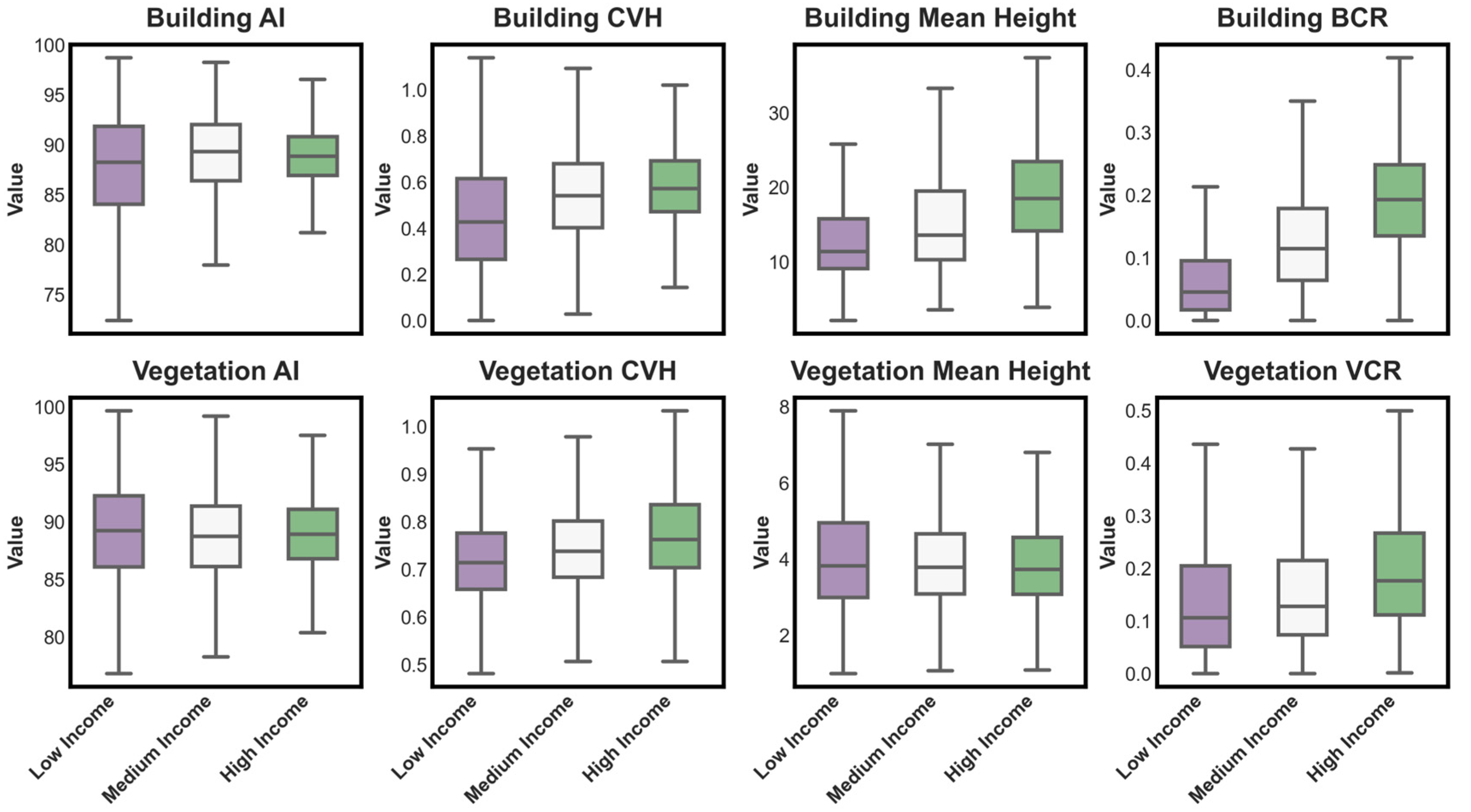
This study compared the distribution of eight physical features across income groups (Low, Medium, and High) to analyze disparities in urban cooling resource allocation (Figure 11). Results indicate that the Vegetation Coverage Ratio (VCR) exhibits a distinct gradient, with high-income neighborhoods possessing significantly greater vegetation stocks than low-income areas. This uneven distribution of vegetation forms a physical basis for heat inequality, as disadvantaged communities face an inherent deficit in cooling resource stocks under high-temperature conditions.

In addition to vegetation quantity, the 3D morphological configuration shows a clear socio-economic gradient. High-income areas exhibit higher values for Building Coverage Ratio (BCR), Building Mean Height, and Vegetation Height Coefficient of Variation (CVH). These findings suggest that higher-income environments possess greater shading potential and spatial volumes, which facilitate solar radiation blocking and thermal buffering. Conversely, low-income communities are characterized by low vegetation cover and limited spatial complexity. These systemic disparities in physical stock reduce the environmental regulatory capacity of these areas during extreme weather events.

3.4.2. Differential Response Efficiency Across Socio-Economic Gradients

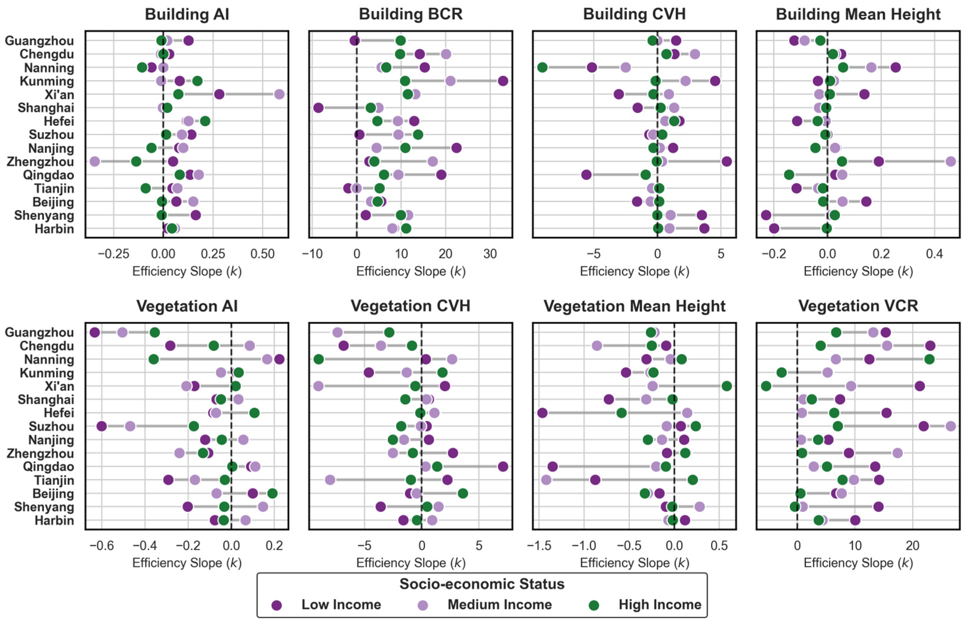
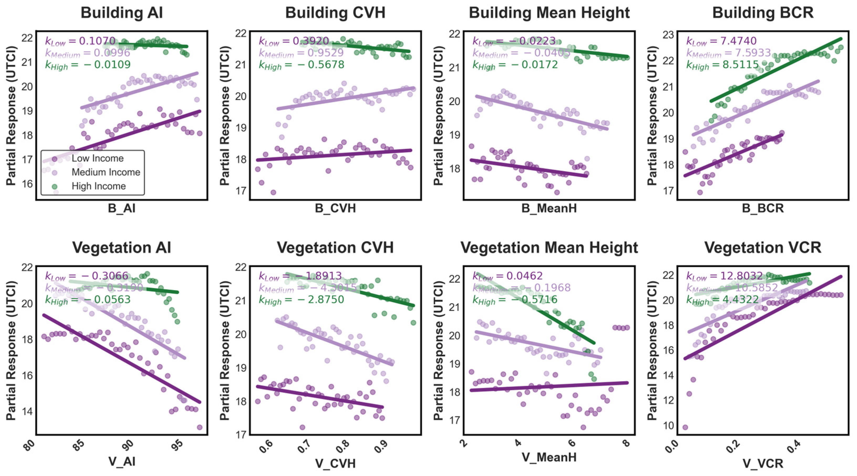
While disparities in resource stocks highlight inequalities in provision, the marginal response of human thermal stress to physical features (Figure 12) reflects distinct variations in regulatory efficiency. The k value represents the marginal response slope where negative signs indicate a cooling effect and positive signs denote a warming effect. A critical finding is the sign reversal of marginal effects for structural complexity. Specifically, Building AI (k_Low = 0.11, k_High = −0.01), Building CVH (k_Low = 0.39, k_High = −0.57), and Vegetation Mean Height (k_Low = 0.05, k_High = −0.57) all exhibit positive slopes in low-income areas but negative slopes in high-income neighborhoods. This indicates that while structural aggregation and height variation facilitate shading and cooling in planned high-income environments, they inadvertently act as heat-trapping mechanisms in high-density, low-income areas. In such disadvantaged contexts, increased building aggregation and vertical complexity likely obstruct localized ventilation and trap long-wave radiation, negating the expected cooling benefits.

Furthermore, the intensity of environmental response varies significantly across socio-economic gradients. High-income environments show greater sensitivity to urban densification, with a steeper positive slope for Building BCR (k_High = 8.51) compared to low-income areas (k_Low = 7.47). This suggests that high-income areas, despite lower absolute stress, are more vulnerable to incremental increases in building density. Conversely, regarding Vegetation VCR, the response gradient for the low-income group (k_Low= 12.80) is nearly triple that of the high-income group (k_High = 4.43). This implies that low-income communities face a far more severe thermal penalty for any reduction in vegetation coverage, highlighting their fragile environmental resilience.

3.4.3. Seasonal Dynamics and Regional Heterogeneity of Response Efficiency

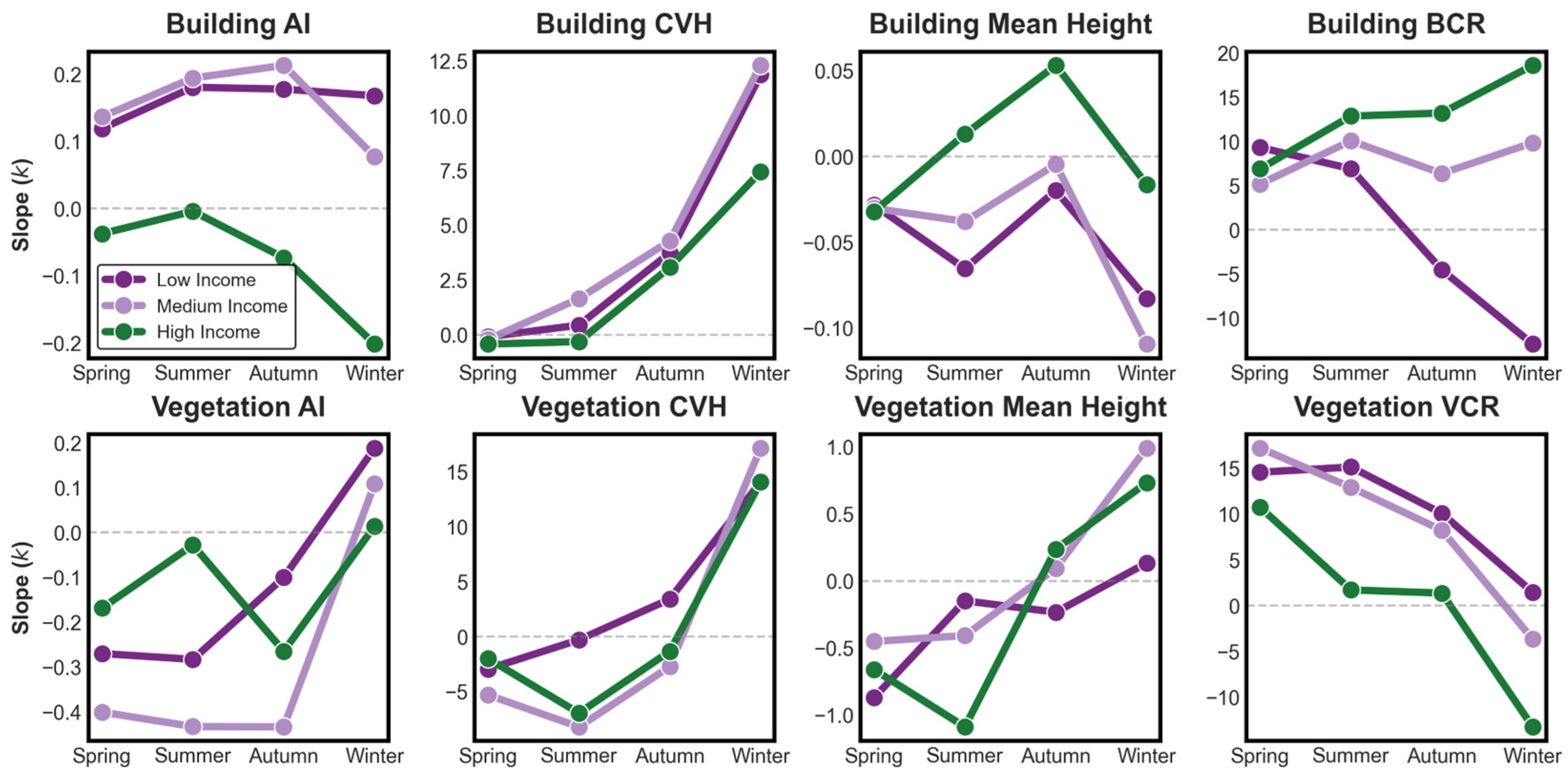
Mechanistic analysis reveals that the response efficiency of physical features exhibits significant temporal instability, characterized by seasonal directional shifts (Figure 13). During summer, vegetation and building morphology in high-income communities demonstrate pronounced negative marginal thermal effects, indicating superior climatic regulatory performance. Conversely, low-income communities experience more intense thermal accumulation in winter, where the marginal warming effect of building mass (Building CVH) is substantially higher (k > 12) than that in high-income groups (k ≈ 7). These seasonal reversals in polarity and variations in the magnitude of k reflect the dynamic complexity of heat inequality, suggesting a systemic attenuation of environmental regulatory capacity in low-income neighborhoods throughout the annual cycle.

Granular analysis across the 15 study cities further identifies significant regional divergence in these efficiency gaps (Figure 14). Southern humid-hot cities (Nanning, Guangzhou, Chengdu) exhibit the most severe efficiency gaps, indicating that unplanned densification in disadvantaged neighborhoods creates localized thermal penalties absent in affluent zones. In contrast, megacities and northern cities (Shanghai, Beijing, Harbin) show converged response patterns, suggesting a more homogenized urban fabric where physical features yield consistent cooling effects regardless of neighborhood income. These divergent patterns dictate that heat mitigation must transition from uniform standards to city-specific strategies: high-divergence cities should focus on structural remediation of unplanned areas, while low-divergence cities should prioritize baseline resource optimization (see

Table A4. Efficiency gaps and divergence types across the 15 study cities.

City	Most Unequal Driver	Max Efficiency Gap	Divergence Type
Xi’an	V_VCR	26.648	High-Divergence
Kunming	B_BCR	22.066	High-Divergence
Chengdu	V_VCR	18.995	High-Divergence
Suzhou	V_VCR	14.883	High-Divergence
Shenyang	V_VCR	14.488	High-Divergence
Qingdao	B_BCR	12.867	High-Divergence
Shanghai	B_BCR	11.712	High-Divergence
Nanjing	B_BCR	11.492	Low-Divergence
Nanning	V_VCR	10.402	Low-Divergence
Guangzhou	B_BCR	10.289	Low-Divergence
Hefei	V_VCR	9.0926	Low-Divergence
Zhengzhou	V_VCR	8.1527	Low-Divergence
Tianjin	B_BCR	7.0764	Low-Divergence
Harbin	V_VCR	6.3243	Low-Divergence
Beijing	V_VCR	6.1559	Low-Divergence

).

3.5. Spatial Contribution Patterns and Precision Identification of Heat Inequality

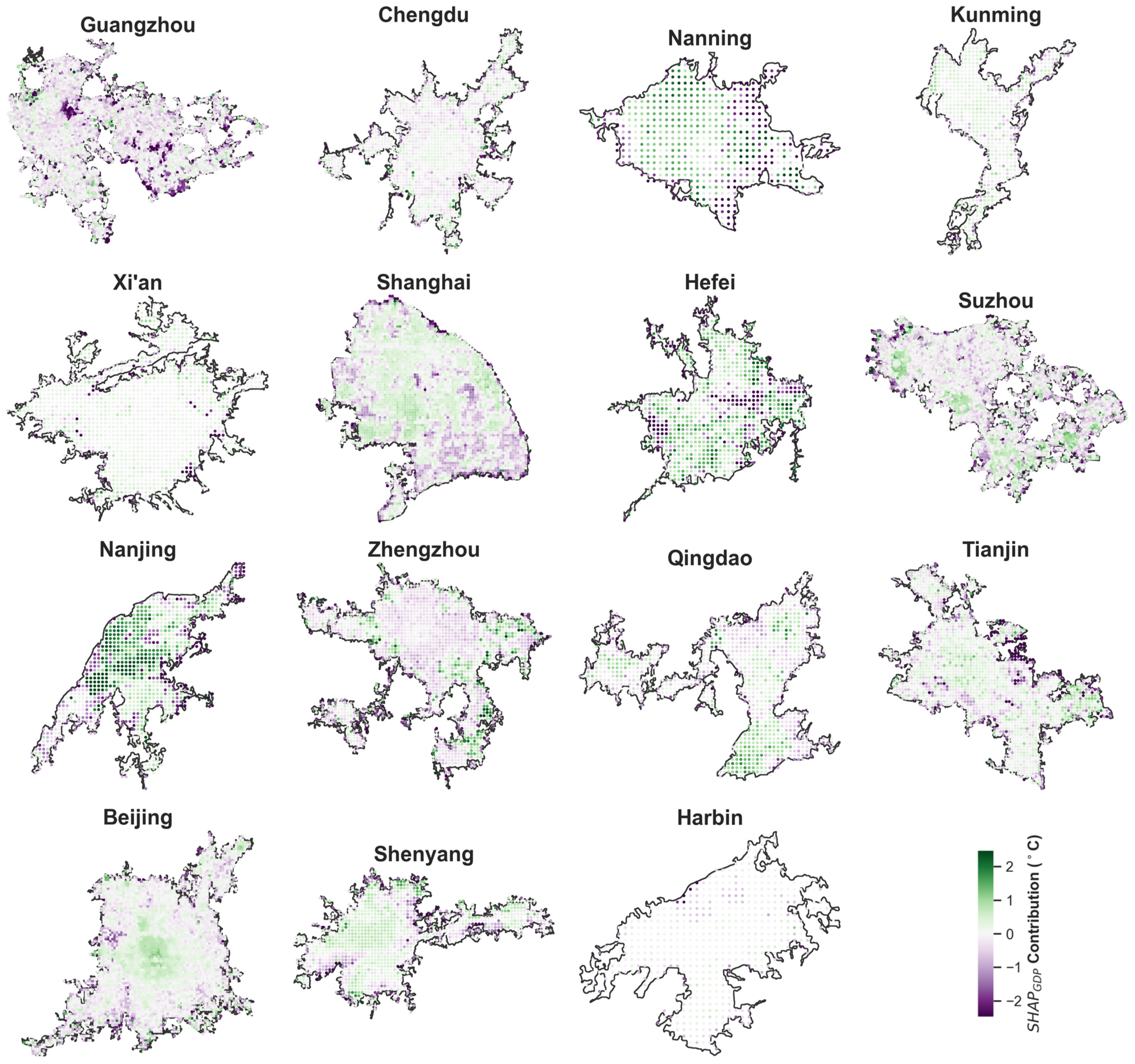
This study employed the GeoShapley algorithm to map the independent spatial contribution of economic levels to human thermal stress (Figure 15). The spatial contribution maps reveal pronounced differentiation between economic status and heat exposure across the 15 study cities. In the core areas of megacities such as Nanjing, Beijing, Shanghai, and Xi’an, economic levels exhibit contiguous positive contributions (darker regions), forming distinct high-exposure hotspots. This indicates a spatial convergence of high-intensity economic development and microclimatic thermal stress, where heat exposure levels rise alongside urban development intensity.

Conversely, in specific zones of cities like Nanning, Guangzhou, and Suzhou, economic levels demonstrate significant negative contributions, suggesting that socio-economic resources can mitigate thermal stress through the optimization of localized physical environments. The coexistence of opposite spatial polarities highlights the geographical complexity of urban heat inequality. Figure 15 serves not only as a global assessment of heat inequality but also as a spatial diagnostic tool for identifying priority areas of environmental injustice. These findings emphasize that advancing urban climate justice requires block-scale efficiency optimization and the implementation of targeted mitigation strategies in high-contribution hotspots.

4. Discussion

4.1. Spatial Association Between Wealth and Heat Exposure in High-Density Cities

Contrary to the empirical findings documented in [15,41], which illustrate a clear divergence between wealth and environmental risk, the high-density urbanization context examined here exhibits a systemic wealth-exposure convergence. We identify a socio-spatial reversal of the traditional Luxury Effect: while affluence in low-density Western contexts typically facilitates thermal mitigation, the centripetal accumulation of wealth in China’s urban cores leads to a positive coupling between economic levels and heat exposure. In this regime, the socio-economic drive for urban centrality outweighs the environmental preference for cooler microclimates, effectively flipping the traditional relationship between wealth and climate risk.

This reversal is driven by the structural coupling of economic status and development intensity. In these high-density systems, higher socio-economic status is physically manifested through residence in high-value, high-intensity urban cores. These areas are characterized by maximized building footprints and complex 3D configurations that fundamentally reshape the radiative environment. Although affluent districts may possess higher vegetation stocks, the localized cooling benefits are neutralized by the overwhelming thermal loads of the built environment. This suggests that in the Global South’s megacities, the capacity of wealth to “buy” environmental quality is constrained by the spatial logic of urban centrality, where the economic benefits of density come at the cost of a significant thermal penalty.

4.2. Seasonal Dynamics and the Amplification Effects of Climatic Forcing

The association between wealth and thermal stress exhibits significant temporal dynamics, indicating that urban heat inequality is not a static spatial pattern but a systematic risk that evolves with climatic forcing. This seasonal trend aligns with the summer peak identified in [13], yet reveals a directional reversal from their reported negative slope to a positive wealth-exposure coupling. Under extreme thermal conditions, the exposure gap between socio-economic strata increases non-linearly, suggesting that climatic environments act as a significant moderator of social differentiation. This dynamic highlights the localized vulnerability of high-density cities during peak summer periods. Relying on annual averages or static assessments tends to underestimate the environmental risks faced by vulnerable populations during climatic extremes. The essence of heat inequality lies in the disproportionate distribution of exposure risks under high environmental stress.

The underlying mechanism for this dynamic involves threshold effects where environmental conditions moderate social differentiation. When background temperature and humidity exceed critical thresholds, the disparity in the capacity of different socio-economic groups to modulate their microenvironments is amplified, leading to a systemic shift in the social exposure deficit. This identifies heat inequality as an environment-sensitive form of social disparity. In the context of increasing extreme weather events driven by climate warming, this exposure gap mediated by climatic forcing is likely to expand. Consequently, urban governance must transition from static resource allocation to proactive temporal intervention, implementing precision strategies during peak inequality periods induced by extreme weather events.

4.3. Mechanistic Analysis of Cooling Resource Stocks and Response Efficiency

The analysis indicates that the drivers of urban heat inequality have transitioned from quantitative disparities in resource provision to a structural decoupling of thermodynamic response logic. Although high-income areas exhibit higher absolute heat exposure, the marginal cooling effects of their environmental features remain significant. This suggests that while their thermal stress is primarily driven by the environmental loads of high-intensity development, their microclimatic regulation mechanisms remain functional. Conversely, low-income communities experience a concurrent deficit in both resource stocks and regulatory performance. This efficiency gap extends social vulnerability from exposure levels to the degradation of environmental regulation mechanisms, suggesting that disadvantaged populations reside in environments where physical features have lost their regulatory capacity due to sub-optimal spatial configurations.

While Nature-based Solutions (NBS) are predominantly categorized as cooling assets in existing literature [42,43], our findings identify a thermal penalty regime where these assets transition into thermal impediments (k > 0). The directional reversal of the marginal response slope k in low-income areas quantifies a regime of failed thermal response, where increasing specific physical inputs yields positive thermal feedback. In high-density, low-income neighborhoods with restricted ventilation, increasing vegetation complexity (CVH) may fail to provide cooling and instead exacerbate human thermal stress by obstructing convective cooling and facilitating near-surface humidity accumulation. These findings characterize heat risk as a structural constraint imposed by spatial configurations. Consequently, mitigation strategies should prioritize the optimization of spatial arrangements—such as building ventilation topology and 3D morphology—to restore the regulatory performance of physical assets in high-density environments.

4.4. Precision Strategies Based on Urban Physical Mechanisms

To provide actionable design parameters, we propose a differential density-control framework based on the varying sensitivities of socio-economic groups. In cities like Xi’an, the thermal sensitivity of low-income areas to Building BCR (k ≈ 30.0) is nearly four times higher than that of high-income zones (k ≈ 8.0), suggesting that even minor densification in disadvantaged neighborhoods triggers severe thermal penalties. Consequently, we recommend a stringent BCR cap (e.g., 40%) for low-income neighborhood redevelopments, coupled with vertical development using reduced building footprints—increasing building mean height (which exhibits a cooling potential of k = −0.02)—to maintain floor-area ratios while optimizing canyon shading and ventilation.

Furthermore, urban greening must shift from quantity-based metrics to connectivity-oriented targets, particularly in vulnerable zones where Vegetation AI is five times more effective at cooling (k = −0.31) than in affluent areas (k = −0.06). Policy should prioritize large-scale connected green corridors over fragmented patches to maximize convective cooling for disadvantaged populations. For humid-hot regions like Nanning, we establish a biomass density (VCR) safety threshold to prevent the reversal of regulatory efficiency. In these contexts, the extreme thermal penalty of VCR in low-income areas (k = 12.80, nearly triple that of high-income zones) dictates that design priorities must transition from increasing vegetation volume to optimizing ventilation topologies, ensuring that nature-based solutions function as cooling mechanisms rather than thermal impediments.

4.5. Limitations

This study provides a mechanistic understanding of urban heat inequality but contains several limitations. First, while the 1 km spatial scale represents the highest-resolution UTCI product currently available, it constrains the analysis of micro-scale shading and convective processes within street canyons. Future research could integrate high-fidelity 3D modeling and micro-climate simulations (e.g., ENVI-met) to quantify the specific contributions of shading geometry to efficiency deviations. Second, while GDP per capita serves as a robust economic proxy for socio-economic status (SES), it does not fully account for fine-grained socio-demographic attributes such as age structure or occupation. Furthermore, gridded GDP may partially reflect commercial intensity and business activity rather than purely residential income patterns. Future research should integrate household-level data to enable a more nuanced social vulnerability assessment. Third, the current analysis focuses on static environmental exposure and does not account for behavioral adaptation mechanisms or human mobility patterns. Specifically, the widespread use of air conditioning and variations in outdoor activity patterns can significantly alter the actual physiological heat stress experienced by different socio-economic groups. While our results establish the physical basis of urban heat inequality, they do not capture individual exposure-trajectories across different microclimates. Future research should integrate high-resolution mobility data and household-level energy consumption patterns to transition from environmental exposure assessment to a comprehensive evaluation of individual physiological heat stress.

5. Conclusions

Urban heat inequality represents a critical barrier to achieving inclusive and resilient climate governance. While traditional assessments predominantly rely on static land surface temperature, they often overlook the dynamic evolution of human thermal stress (UTCI) and the divergent regulatory efficiencies of cooling features across socio-economic contexts. By integrating multi-source datasets from 15 Chinese cities and employing a machine learning framework with GeoShapley interpretation, this study systematically quantifies the driving mechanisms of heat inequality across three dimensions: spatio-temporal evolution, environmental amplification, and efficiency bias. These findings characterize the non-linear coupling between socio-economic status and thermal stress in high-density urban environments, establishing a framework for precision climate risk identification.

The results confirm a prevalent positive spatial coupling between GDP per capita and UTCI in high-density Chinese cities, deviating from the luxury effect observed in low-density urban contexts. High-income areas exhibit significantly higher absolute thermal stress, driven by high-intensity development, radiative accumulation within deep street canyons, and the attenuation of convective cooling. Furthermore, the intensity of heat inequality fluctuates significantly with environmental forcing. Background temperature and humidity act as moderating variables that trigger a non-linear expansion of the social exposure deficit during summer, highlighting the heightened sensitivity of urban thermal systems to climatic stress.

Beyond quantitative disparities in resource provision, this study identifies a systemic attenuation of environmental regulatory performance in low-income communities. Physical features in these areas, such as vegetation 3D complexity, exhibit a directional reversal in thermal response polarity due to structural constraints within the built environment. This shift in the response slope k suggests that the essence of heat inequality lies in the degradation of thermodynamic regulatory logic, where incremental resource inputs may yield positive thermal feedback under sub-optimal spatial configurations. Future research will prioritize micro-scale physical processes within street canyons and integrate human mobility data to establish dynamic exposure assessment frameworks, providing a scientific basis for targeted interventions to mitigate urban climate injustice.

References

1. Watts, N.; Amann, M.; Ayeb-Karlsson, S.; Belesova, K.; Bouley, T.; Boykoff, M.; Byass, P.; Cai, W.; Campbell-Lendrum, D.; Chambers, J.; et al. The Lancet Countdown on health and climate change: From 25 years of inaction to a global transformation for public health. Lancet 2018, 391, 581–630. [Google Scholar] [CrossRef]
2. Chakraborty, T.C.; Qian, Y.; Li, J.; Leung, L.R.; Sarangi, C. Daytime urban heat stress in North America reduced by irrigation. Nat. Geosci. 2025, 18, 57–64. [Google Scholar] [CrossRef]
3. Harmay, N.S.M.; Choi, M. The urban heat island and thermal heat stress correlate with climate dynamics and energy budget variations in multiple urban environments. Sustain. Cities Soc. 2023, 91, 104422. [Google Scholar] [CrossRef]
4. Yadav, N.; Rajendra, K.; Awasthi, A.; Singh, C.; Bhushan, B. Systematic exploration of heat wave impact on mortality and urban heat island: A review from 2000 to 2022. Urban Clim. 2023, 51, 101622. [Google Scholar] [CrossRef]
5. Salazar-Miranda, A.; Conzelmann, C.; Phan, T.; Hoffman, J. Long-term effects of redlining on climate risk exposure. Nat. Cities 2024, 1, 436–444. [Google Scholar] [CrossRef]
6. Guo, A.; Yue, W.; Yang, J.; Li, M. Assessing inequality in population exposure of urban heat across China’s major cities. Appl. Geogr. 2025, 185, 103788. [Google Scholar] [CrossRef]
7. Liu, Q.; Hang, T. Reassessing urban heat exposure inequity: Bridging subjective perception and objective conditions for a more accurate understanding. Sustain. Cities Soc. 2025, 130, 106657. [Google Scholar] [CrossRef]
8. Shreevastava, A.; Hulley, G.; Prasanth, S.; Chakraborty, T.C.; Ramos Aguilera, D.; Twomey Sanders, K.; Yin, Y. Contemporary income inequality outweighs historic redlining in shaping intra-urban heat disparities in Los Angeles. Nat. Commun. 2025, 16, 4950. [Google Scholar] [CrossRef]
9. Hope, D.; Gries, C.; Zhu, W.; Fagan, W.F.; Redman, C.L.; Grimm, N.B.; Nelson, A.L.; Martin, C.; Kinzig, A. Socioeconomics drive urban plant diversity. Proc. Natl. Acad. Sci. USA 2003, 100, 8788–8792. [Google Scholar] [CrossRef] [PubMed]
10. Gerrish, E.; Watkins, S.L. The relationship between urban forests and income: A meta-analysis. Landsc. Urban Plan. 2018, 170, 293–308. [Google Scholar] [CrossRef] [PubMed]
11. Chakraborty, T.; Hsu, A.; Manya, D.; Sheriff, G. Disproportionately higher exposure to urban heat in lower-income neighborhoods: A multi-city perspective. Environ. Res. Lett. 2019, 14, 105003. [Google Scholar] [CrossRef]
12. Olsen, J.R.; Niedzwiedz, C.; Nicholls, N.; Wheeler, B.W.; Ho, F.K.; Pell, J.P. Sociodemographic and geographic inequalities in exposure to projected hot and extreme summer days in England: A nationwide socio-spatial analysis. Environ. Int. 2025, 197, 109351. [Google Scholar] [CrossRef] [PubMed]
13. Yin, Y.; He, L.; Wennberg, P.O.; Frankenberg, C. Unequal exposure to heatwaves in Los Angeles: Impact of uneven green spaces. Sci. Adv. 2023, 9, eade8501. [Google Scholar] [CrossRef]
14. Zeng, P.; Chen, C.; Sun, F.; Liu, Y.; Zhang, X.; Che, Y. Surface temperature change amplifies social inequality in heat exposure? Evidence from Shanghai, China. Environ. Chall. 2024, 17, 101048. [Google Scholar] [CrossRef]
15. Marcińczak, S.; Iglesias-Pascual, R.; Kopeć, D.; Wróbel, K.; Mooses, V. Landscapes of thermal inequality: Exploring patterns of climate justice across multiple spatial scales in Spain. Landsc. Urban Plan. 2025, 254, 105255. [Google Scholar] [CrossRef]
16. Zhu, Y.; Myint, S.W.; Schaffer-Smith, D.; Tong, D.; Zhou, Y.; Li, Y.; Muenich, R.L. Rising Environmental Inequalities and Their Relationship to Racial and Socioeconomic Disparities in the US Southwest. Environ. Sci. Technol. 2025, 59, 17534–17544. [Google Scholar] [CrossRef]
17. Abuwaer, N.; Ullah, S.; Al-Ghamdi, S.G. Establishing the nexus between urban walkability and thermal comfort in a changing climate. Nat. Cities 2025, 2, 801–811. [Google Scholar] [CrossRef]
18. Jendritzky, G.; De Dear, R.; Havenith, G. UTCI—Why another thermal index? Int. J. Biometeorol. 2012, 56, 421–428. [Google Scholar] [CrossRef]
19. Stewart, I.D.; Oke, T.R. Local climate zones for urban temperature studies. Bull. Am. Meteorol. Soc. 2012, 93, 1879–1900. [Google Scholar] [CrossRef]
20. Deng, Q.; Liu, G.; Xue, N.; Chang, W.; Li, Z.; Yang, Q.; Sohail, S.; Su, M. An Efficient 3D Morphological Analysis Framework for Pedestrian-Level Thermal Stress Assessment in Megacities: Integrating Large-Scale Modeling and Physical Simulation. Sustain. Cities Soc. 2026, 139, 107229. [Google Scholar] [CrossRef]
21. Wang, Y.; He, Z.; Zhai, W.; Wang, S.; Zhao, C. How do the 3D urban morphological characteristics spatiotemporally affect the urban thermal environment? A case study of San Antonio. Build. Environ. 2024, 261, 111738. [Google Scholar] [CrossRef]
22. Yan, X.; Wang, Y.; Luo, X.; Zhou, D. Assessing Urban Thermal Inequity for the Elderly in Relation to 2D/3D Urban Built Environment. Sustain. Cities Soc. 2026, 136, 107116. [Google Scholar] [CrossRef]
23. Zhang, T.; Sun, Y.; Yin, L.; Tian, Y.; Sun, Y.; Zhang, B. Examining heat risk inequality from the perspective of urban resilience. Sustain. Cities Soc. 2025, 131, 106743. [Google Scholar] [CrossRef]
24. Shen, Y.; Kong, W.; Fei, F.; Chen, X.; Xu, Y.; Huang, C.; Yao, J. Stereoscopic urban morphology metrics enhance the nonlinear scale heterogeneity modeling of UHI with explainable AI. Urban Clim. 2024, 56, 102006. [Google Scholar] [CrossRef]
25. Wu, W.-B.; Yu, Z.-W.; Ma, J.; Zhao, B. Quantifying the influence of 2D and 3D urban morphology on the thermal environment across climatic zones. Landsc. Urban Plan. 2022, 226, 104499. [Google Scholar] [CrossRef]
26. Chen, J.; Zhan, W.; Du, P.; Li, L.; Li, J.; Liu, Z.; Huang, F.; Lai, J.; Xia, J. Seasonally disparate responses of surface thermal envi-ronment to 2D/3D urban morphology. Build. Environ. 2022, 214, 108928. [Google Scholar] [CrossRef]
27. Gao, Y.; Zhao, J.; Han, L. Quantifying the nonlinear relationship between block morphology and the surrounding thermal environment using random forest method. Sustain. Cities Soc. 2023, 91, 104443. [Google Scholar] [CrossRef]
28. Oukawa, G.Y.; Krecl, P.; Targino, A.C. Fine-scale modeling of the urban heat island: A comparison of multiple linear regression and random forest approaches. Sci. Total Environ. 2022, 815, 152836. [Google Scholar] [CrossRef]
29. He, J.; Shi, Y.; Xu, L.; Lu, Z.; Feng, M.; Tang, J.; Guo, X. Exploring the scale effect of urban thermal environment through XGBoost model. Sustain. Cities Soc. 2024, 114, 105763. [Google Scholar] [CrossRef]
30. Hu, C.; Zeng, H. Decoding spatial patterns of urban thermal comfort: Explainable machine learning reveals drivers of thermal perception. Environ. Impact Assess. Rev. 2025, 114, 107895. [Google Scholar] [CrossRef]
31. Zhang, M.; Zhou, D.; Xu, D.; Liu, K.; Gu, Z.; Yang, Y.; Zhang, Q.; Chen, L. How do built environment factors influence urban heat islands across local climate zones? Evidence from an interpretable XGBoost-SHAP model. Sustain. Cities Soc. 2025, 136, 107078. [Google Scholar] [CrossRef]
32. Kim, M.-H. Unpacking the Vertical City: Interaction Effects of Urban Forms on Temperatures Using SHAP. Sustain. Cities Soc. 2025, 136, 107061. [Google Scholar] [CrossRef]
33. Li, Z. GeoShapley: A game theory approach to measuring spatial effects in machine learning models. Ann. Assoc. Am. Geogr. 2024, 114, 1365–1385. [Google Scholar] [CrossRef]
34. Zhang, X.; Hu, J.; Xia, T.; Mao, Y.; Li, X.; Hu, C.; Zhang, J. Cooling varies with green space characteristics: Unraveling nonlinear spatial heterogeneity in cooling effects of urban green spaces with geographic explainable AI. Environ. Impact Assess. Rev. 2026, 119, 108401. [Google Scholar] [CrossRef]
35. Chen, Y.; Ye, Y.; Liu, X.; Yin, C.; Jones, C.A. Examining the nonlinear and spatial heterogeneity of housing prices in urban Beijing: An application of GeoShapley. Habitat Int. 2025, 162, 103439. [Google Scholar] [CrossRef]
36. Foroutan, E.; Hu, T.; Li, Z. Revealing key factors of heat-related illnesses using geospatial explainable AI model: A case study in Texas, USA. Sustain. Cities Soc. 2025, 122, 106243. [Google Scholar] [CrossRef]
37. Yang, Z.; Peng, J.; Liu, Y.; Jiang, S.; Cheng, X.; Liu, X.; Dong, J.; Hua, T.; Yu, X. GloUTCI-M: A global monthly 1 km Universal Thermal Climate Index dataset from 2000 to 2022. Earth Syst. Sci. Data 2024, 16, 2407–2424. [Google Scholar] [CrossRef]
38. Kummu, M.; Kosonen, M.; Masoumzadeh Sayyar, S. Downscaled gridded global dataset for gross domestic product (GDP) per capita PPP over 1990–2022. Sci. Data 2025, 12, 178. [Google Scholar] [CrossRef] [PubMed]
39. Che, Y.; Li, X.; Liu, X.; Wang, Y.; Liao, W.; Zheng, X.; Zhang, X.; Xu, X.; Shi, Q.; Zhu, J.; et al. 3D-GloBFP: The first global three-dimensional building footprint dataset. Earth Syst. Sci. Data 2024, 16, 5357–5374. [Google Scholar] [CrossRef]
40. Tolan, J.; Yang, H.-I.; Nosarzewski, B.; Couairon, G.; Vo, H.V.; Brandt, J.; Spore, J.; Majumdar, S.; Haziza, D.; Vamaraju, J.; et al. Very high resolution canopy height maps from RGB imagery using self-supervised vision transformer and convolutional decoder trained on aerial lidar. Remote. Sens. Environ. 2024, 300, 113888. [Google Scholar] [CrossRef]
41. Anguelovski, I.; Kotsila, P.; Lees, L.; Triguero-Mas, M.; Calderón-Argelich, A. From heat racism and heat gentrification to urban heat justice in the USA and Europe. Nat. Cities 2025, 2, 8–16. [Google Scholar] [CrossRef]
42. Sowińska-Świerkosz, B.; García, J. What are Nature-based solutions (NBS)? Setting core ideas for concept clarification. Nat.-Based Solut. 2022, 2, 100009. [Google Scholar] [CrossRef]
43. Dong, X.; Ye, Y.; Su, D.; Haase, D.; Lausch, A. Optimizing urban tree species composition to maximize nature-based solutions. npj Urban Sustain. 2026, 6, 47. [Google Scholar] [CrossRef]
Figure 1. Analytical framework for assessing urban heat inequality and cooling efficiency bias.
Buildings 16 01861 g001
Figure 2. Spatial correlation between UTCI and GDP across 15 Chinese cities. Statistical significance is denoted as follows: * p < 0.05 and *** p < 0.001.
Buildings 16 01861 g002
Figure 3. Seasonal evolution and regional variations of ∆UTCI across 15 Chinese cities. The green shaded area represents the 95% confidence interval.
Buildings 16 01861 g003
Figure 4. Spatio-temporal evolution of the correlation between UTCI and log10(GDP) across 15 Chinese cities. Grey dots represent individual observations; black circles indicate outliers; the red dashed line denotes zero; colors are used to distinguish months and cities for visual clarity.
Buildings 16 01861 g004
Figure 5. Monthly variations in regression slopes and Pearson r for 15 Chinese cities.
Buildings 16 01861 g005
Figure 6. Sensitivity of thermal inequality intensity (Slope) to background climatic variables.
Buildings 16 01861 g006
Figure 7. Synergistic effects of key environmental factors on urban thermal inequality intensity. The size of each circle represents the interaction strength.
Buildings 16 01861 g007
Figure 8. Performance benchmarking of machine learning algorithms for urban UTCI simulation.
Buildings 16 01861 g008
Figure 9. Seasonal stability and global feature importance of the optimized XGBoost model. The red shaded area represents the 95% confidence interval.
Buildings 16 01861 g009
Figure 10. Monthly evolution of feature contributions for environmental, physical, and socio-economic drivers based on GeoShapley.
Buildings 16 01861 g010
Figure 11. Distribution of building morphology and vegetation features across socio-economic groups.
Buildings 16 01861 g011
Figure 12. Heterogeneity in marginal thermal effects of physical features across socio-economic groups.
Buildings 16 01861 g012
Figure 13. Seasonal evolution of marginal thermal response slopes (k) for urban physical features across income strata.
Buildings 16 01861 g013
Figure 14. Inter-city heterogeneity in the efficiency gap between socio-economic groups.
Buildings 16 01861 g014
Figure 15. Spatial heterogeneity of GDP contribution to urban thermal stress across 15 cities in July.
Buildings 16 01861 g015
Disclaimer/Publisher’s Note: The statements, opinions and data contained in all publications are solely those of the individual author(s) and contributor(s) and not of MDPI and/or the editor(s). MDPI and/or the editor(s) disclaim responsibility for any injury to people or property resulting from any ideas, methods, instructions or products referred to in the content.