Stochastic Optimal Control for Uncertain Structural Systems Under Random Excitations Based on Bayes Optimal Estimation

Abstract

Stochastic vibration control of uncertain structures under random loading is an important problem and its minimax optimal control strategy remains to be developed. In this paper, a stochastic optimal control strategy for uncertain structural systems under random excitations is proposed, based on the minimax stochastic dynamical programming principle and the Bayes optimal estimation method with the combination of stochastic dynamics and Bayes inference. The general description of the stochastic optimal control problem is presented including optimal parameter estimation and optimal state control. For the estimation, the posterior probability density conditional on observation states is expressed using the likelihood function conditional on system parameters according to Bayes’ theorem. The likelihood is replaced by the geometrically averaged likelihood, and the posterior is converted into its logarithmic expression to avoid numerical singularity. The expressions of state statistics are derived based on stochastic dynamics. The statistics are further transformed into those conditional on observation states based on optimal state estimation. Then, the obtained posterior will be more reliable and accurate, and the optimal estimation will greatly reduce uncertain parameter domains. For the control, the minimax strategy is designed by minimizing the performance index for the worst-parameter system, which is obtained by maximizing the performance index based on game theory. The dynamical programming equation for the uncertain system is derived according to the minimax stochastic dynamical programming principle. The worst parameters are determined by the maximization of the equation, and the optimal control is determined by the minimization of the resulting equation. The minimax optimal control by combining the Bayes optimal estimation and minimax stochastic dynamical programming will be more effective and robust. Finally, numerical results for a five-story frame structure under random excitations show the control effectiveness of the proposed strategy.

1. Introduction

Stochastic vibration control of uncertain structures under random loading is an important research subject [1,2,3,4,5,6,7,8], addressing, for example, the vibration mitigation of building structures under wind and earthquake loading. The control design is based on a structural model, and the model parameters are uncertain; they need to be estimated, and the estimated results are approximate. Then, the stochastic control of uncertain structures includes two problems: uncertain parameter estimation and robust vibration control. Structural parameter estimation has been studied and several estimation methods have been proposed [9,10,11,12,13,14,15,16]. For example, this is a probabilistic estimation problem on uncertain structures under random excitations using only measured stochastic responses. Bayes’ theorem was used to express the posterior probability density by the likelihood function for parameter estimation. The likelihood function was calculated based on special assumptions on conditional probability density with hyper parameters, Kullback–Leibler divergence or Monte-Carlo numerical simulation [17,18,19,20,21,22,23,24,25,26,27,28,29,30,31,32,33,34,35,36,37]. On the other hand, the stochastic vibration control of uncertain structures has been studied, and several control strategies have been proposed [38,39,40,41,42,43,44,45,46,47,48,49,50,51,52,53,54,55,56]. For example, this structural control implementation requires the designed control to have certain robustness about uncertain parameters. The stochastic robustness of control systems with uncertain parameters has been analyzed [57,58]. Different from the conventional non-optimal robust control, the minimax optimal control for uncertain stochastic systems has been proposed as an optimal robust control [59,60,61,62,63,64,65,66,67]. The optimal control was designed for the worst system with certain constraints which depend on uncertain parameters based on game theory. The optimal H∞ control can be regarded as another minimax control, and a machine learning algorithm was also used to increase robustness. At present, the two categories of studies with methods (Bayes estimation and minimax control) are mostly independent. However, the minimax vibration control depends on the uncertain parameter domains, and the parameter domains depend on estimated results. The uncertain structural parameters will vary with the surroundings, for example, temperature and material degradation. Therefore, a study on the stochastic vibration control of uncertain structures under random loading needs to reasonably combine minimax control with parameter estimation. In particular, the optimal parameter estimation method for uncertain structural systems under random excitations has been proposed recently, which has better estimation accuracy [68]. 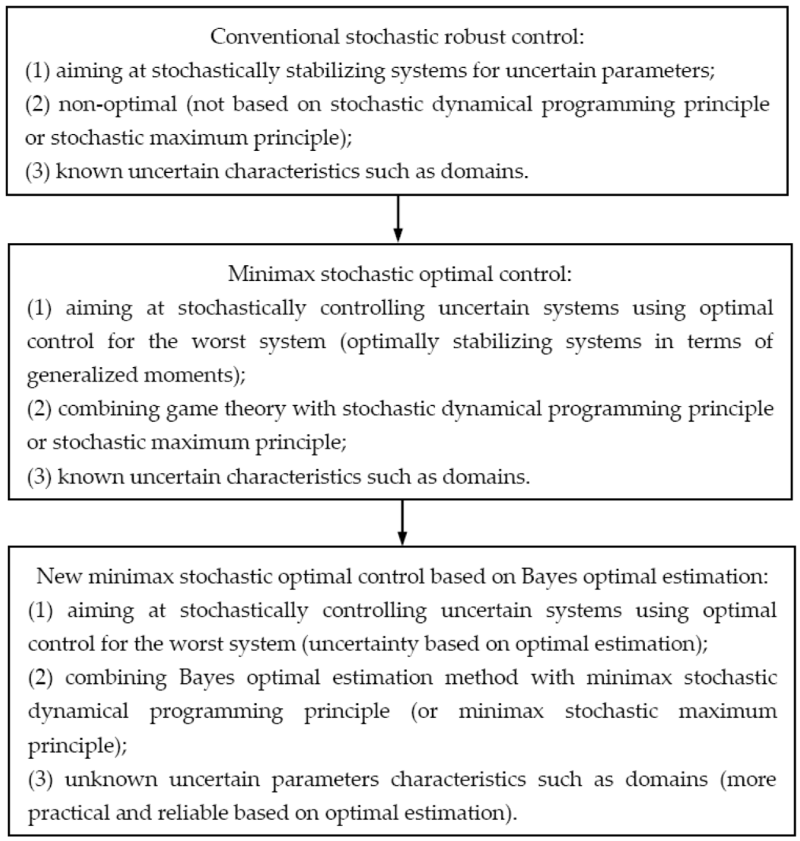The optimal vibration control strategy for uncertain structural systems under random excitations has been proposed, and the numerical results of examples showed better control effectiveness, but the control effectiveness depends on uncertain parameter domains or boundaries [65,66]. Then, a new stochastic optimal vibration control for uncertain structural systems by combining the minimax optimal control strategy with optimal parameter estimation method remains to be developed further (the development with characteristics is shown in the following Scheme 1).

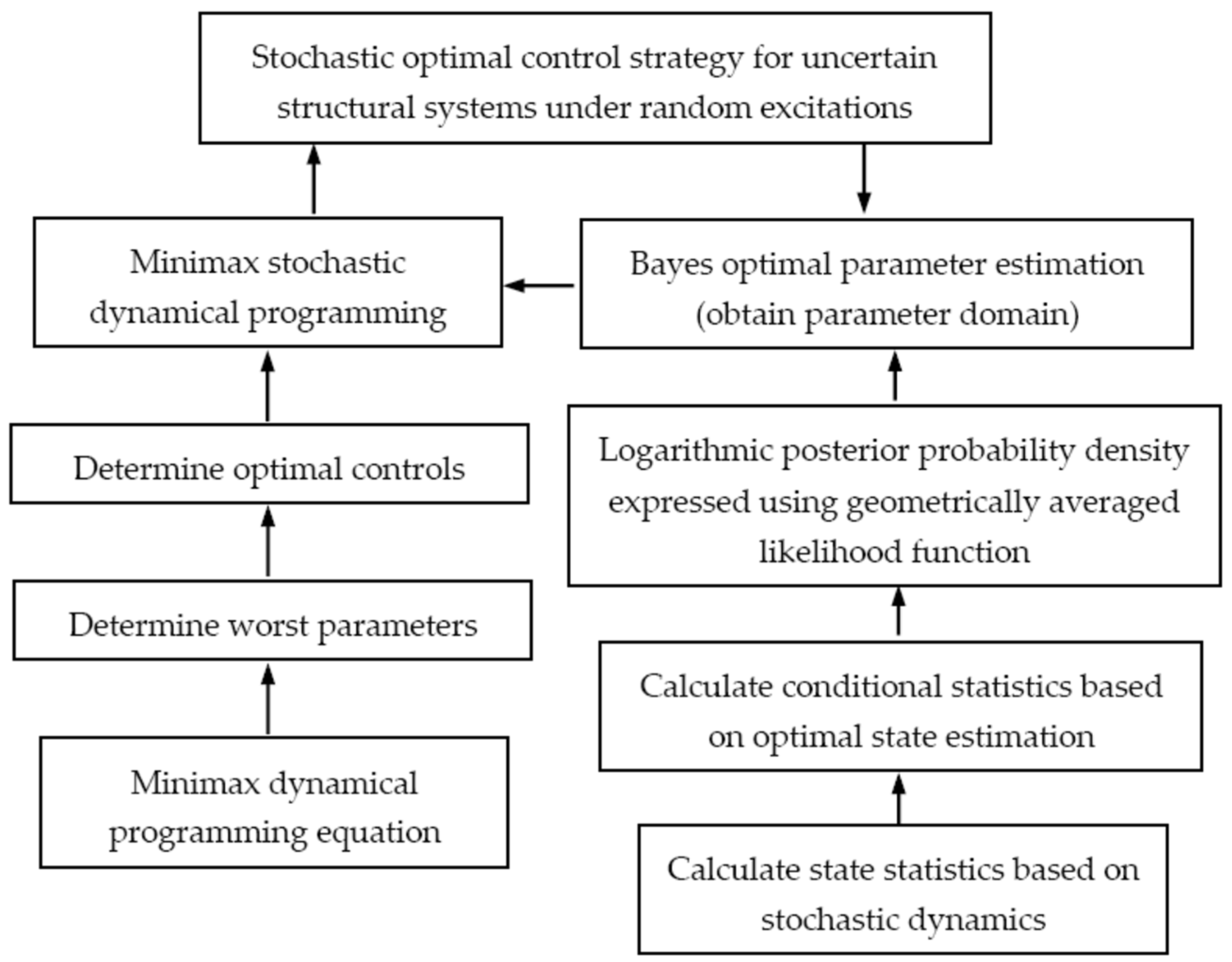
The present paper proposes a stochastic optimal control strategy for uncertain structural systems under random excitations by combining the minimax stochastic dynamical programming principle with Bayes optimal estimation, as shown in the following Scheme 2. First, the general description of the stochastic optimal control problem for uncertain structural systems under random excitations is presented based on game theory, including optimal parameter estimation and optimal state control. Then, the control problem is separated into an optimal parameter estimation problem and an optimal state control problem. Second, for the optimal parameter estimation, Bayes’ theorem is applied to express the posterior probability density conditional on observation states by the likelihood function conditional on system parameters. The likelihood function as joint distribution density is replaced by the geometrically averaged likelihood function, and the posterior probability density is converted into its logarithmic expression accordingly to avoid numerical singularity. Further, the expressions of the state statistics including means and covariances are derived based on stochastic dynamics theory. Then, the state statistics are transformed into those conditional on observation states based on the optimal state estimation. By using conditional statistics, the posterior probability density can be obtained, which will be more reliable and accurate for parameter estimation. The estimated parameters are relatively accurate, which greatly reduce the uncertain parameter domains and improve the identified system for control design. Third, for the optimal state control, the minimax control is designed as the optimal control by minimizing the performance index for the system with the worst parameters obtained by maximizing the performance index based on game theory. According to the minimax stochastic dynamical programming principle, a dynamical programming equation for the uncertain systems is derived. The worst parameters are determined by the maximization of the equation. Then, the optimal control for the worst-parameter system is determined by the minimization of the equation with the worst parameters. The minimax optimal control, by combining Bayes optimal estimation and minimax stochastic dynamical programming, will be more effective and robust. Therefore, a stochastic optimal control strategy for uncertain structural systems under random excitations is developed. Finally, the proposed control strategy is used to the vibration mitigation of a five-story frame structure under random base excitations. Only stochastic responses are used for parameter estimation and feedback control. Numerical results show that the stochastic responses of the uncertain structure under white noise and earthquake excitations can be effectively controlled. The control effectiveness is robust about uncertain parameters and estimation errors. The effects of other control parameters on the control effectiveness are also discussed.

2. Optimal Control Problem on Uncertain Stochastic Structure System

Consider a structural system with control under random excitation, such as a building. Its dynamic equation can be expressed as

$$M{\displaystyle \frac{{\mathrm{d}}^{2}X}{\mathrm{d}{t}^2}}+C{\displaystyle \frac{\mathrm{d}X}{\mathrm{d}t}}+KX=F(t)+B_{0}U$$

(1)

where X is the n-dimensional displacement response vector; M, C and K are the n×n-dimensional mass, stiffness and damping matrices, respectively; F is the n-dimensional random excitation vector; U is the m-dimensional control vector; B₀ is the control placement matrix; and t is time. In general, the system mass is determinable, and stiffness and damping are uncertain parameters to be estimated. The excitation is generally random due to complicated surroundings, and its sample is unknown. Many practical excitations can be represented by filtering Gaussian white noises. Incorporating the filter in the system leads to an augmented system with white noise excitation. Therefore, the excitation in Equation (1) is assumed as Gaussian white noise. Only stochastic system responses at the present and previous instants can be obtained by measurement. The feedback control will be designed as a function of the measured responses.

Rewrite Equation (1) in the form

$${\displaystyle \frac{\mathrm{d}Z}{\mathrm{d}t}}=AZ+G(t)+BU$$

(2)

where state vector Z, uncertain parameter matrix A, random excitation vector G and control placement matrix B are

$$Z=\left\{\begin{array}{c}X\\ \mathrm{d}X/\mathrm{d}t\end{array}\right\}, A=\left[\begin{array}{cc}0& I\\ -M^{-1}K& -M^{-1}C\end{array}\right], G=\left\{\begin{array}{c}0\\ M^{-1}F\end{array}\right\}, B=\left\{\begin{array}{c}0\\ M^{-1}{B}_0\end{array}\right\}$$

(3)

in which I is the identity matrix.

The state of the uncertain stochastic system (2) can be observed by measurement, and the uncertain system parameters need to be estimated. The control will be determined under observation and estimation. Then, the stochastic optimal control problem for the uncertain system includes two parts: optimal parameter estimation and optimal state control. Based on game theory, it can be described by

$$\underset{U\in {\Omega }_c}{\min }\underset{\phi \in {\Omega }_p}{\min }\{J(U,\Delta \phi \left|Z(t_1)\sim Z(t_2)\right.)\}$$

(4)

where φ is the uncertain parameter vector, Δφ is the estimation error vector, Z(t₁) and Z(t₂) are the measured states at the starting and end instants of a finite time process, Ω_c and Ω_p are the control and parameter domains, respectively, and J is the performance index. For a finite time process, the uncertain parameters can be regarded as unchanged, and the control in the previous interval has been determined. Then, problem (4) can be separated into the following optimal parameter estimation and optimal state control:

$$\underset{\phi \in {\Omega }_p}{\min }\{J_e(\Delta \phi \left|Z(t_1)\sim Z(t_2),U^{*}\right.)\}$$

(5)

$$\underset{U\in {\Omega }_c}{\min }\{J_c(U\left|Z(t_0)\sim Z(t_f),{\phi }^{*}\right.)\}$$

(6)

The stochastic optimal estimation is to optimally determine the values of the uncertain parameters by using the observed states in a finite time interval. The parameters are estimated by minimizing the total error between estimating and factual values. The performance index of the optimal estimation is generally expressed as the conditional mean [2]:

$$J_e(\Delta \phi \left|Z(t_1)\sim Z(t_2),U^{*}\right.)=E\{L_e(\Delta \phi )\left|Z(t_1)\sim Z(t_2)\right.\}$$

(7)

where $\Delta \phi ={\phi }^{*}-\phi$, φ* is the optimally estimated parameter vector, U* is the previously determined optimal control vector, L_e(.) is a positive definite functional with L_e(0) = 0 and E{.} denotes the expectation operation. States Z are determined by Equation (2) and obtained by measurement. The optimal estimation is represented by [68]

$$J_e(\Delta \phi \left|Z(t_1)\sim Z(t_2),U^{*}\right.)\stackrel{\phi ={\phi }^{*}}{\to }\underset{\phi \in {\Omega }_p}{\min }$$

(8)

The estimated parameters can be determined according to Bayes optimal estimation.

The stochastic optimal control is to optimally determine a function of the system control under the estimated parameters and observed states in a finite time interval. The control is obtained by minimizing the performance index under observation and estimation. The performance index of the optimal control is generally expressed as [2]

$$J_c(U\left|Z(t_0)\sim Z(t_f),{\phi }^{*}\right.)=E\{{\displaystyle {\int }_{t_0}^{t_f}{L}_c(Z,{\phi }^{*},U)\mathrm{d}t}+\Psi (Z(t_f))\}$$

(9)

where t₀ and t_f are the initial and terminal times of control, respectively, L_c(.) is a positive definite functional and Ψ is the terminal cost. The estimation time interval [t₁, t₂] moves with time, but t₂ is smaller than the control terminal time t_f. Then, U is the control to be determined presently. The optimal control for the estimated system (2) with index (9) is represented by [38]

$$J_c(U\left|Z(t_0)\sim Z(t_f),{\phi }^{*}\right.)\stackrel{U=U^{*}}{\to }\underset{U\in {\Omega }_c}{\min }$$

(10)

where * denotes the optimal value. The optimal control can be determined according to the stochastic dynamical programming principle with the minimax strategy.

The stochastic optimal feedback control strategy for a structural system under random excitations based on optimal parameter estimation with observed states, by combining Bayes optimal estimation and minimax stochastic dynamical programming, is described in the following two sections.

3. Bayes Optimal Estimation Method for Uncertain System Parameters

The optimal estimation (8) can be calculated by using the posterior probability density conditional on observed states. Bayes’ theorem is firstly applied to convert the posterior probability density into another represented by the likelihood function conditional on system parameters. For the finite time process, the posterior probability density is expressed as

$$p(\phi \left|Z(t_1)\sim Z(t_2)\right.)={\displaystyle \frac{p(Z(t_1)\sim Z(t_2)\left|\phi \right.)p(\phi )}{p(Z(t_1)\sim Z(t_2))}}$$

(11)

where p(Z(t₁)~Z(t₂)|φ) is the likelihood function, p(φ) is the prior probability density and p(Z(t₁)~Z(t₂)) is the state probability density which is independent of parameters and can be regarded as a normalization coefficient.

Divide the time interval [t₁, t₂] into N equal subintervals. Using conditional probability densities, the likelihood function as a joint probability density is expressed as [68]

$$p(Z(t_1)\sim Z(t_2)\left|\phi \right.)={\displaystyle \prod _{i=1}^{N+1}p(Z({\tau }_i)\left|\phi ,Z(t_1)\sim Z({\tau }_{i-1})\right.)}$$

(12)

where p(Z(τ₁)|φ,Z(t₁)~Z(τ₀)) = p(Z(t₁)|φ) and p(Z(τ_i)|φ,Z(t₁)~Z(τ_i−1)) is the instant-τ_i state probability density conditional on the previous states. However, the right-hand side of Equation (12) is the product of infinite terms for the finite time process, which will result in numerical singularity. Then, the geometrically averaged likelihood function p_ga is used, and the posterior probability density (11) is re-expressed as

$$p(\phi \left|Z(t_1)\sim Z(t_2)\right.)={[p_{ga}(Z(t_1)\sim Z(t_2)\left|\phi \right.)]}^{N+1}{\displaystyle \frac{p(\phi )}{\lambda }}$$

(13)

$$p_{ga}(Z(t_1)\sim Z(t_2)\left|\phi \right.)={[{\displaystyle \prod _{i=1}^{N+1}p(Z({\tau }_i)\left|\phi ,Z(t_1)\sim Z({\tau }_{i-1})\right.)}]}^{1/(N+1)}$$

(14)

where λ is the normalization constant. The posterior probability density (13) can be replaced by its logarithm.

Further, the state probability density conditional on the previous states in Equation (14) can be calculated based on the stochastic dynamics theory and optimal state estimation method. For system (2) with certain parameters, states are Gaussian processes under Gaussian random excitations. The state probability density is determined by the second-order statistics. According to stochastic dynamics [69], the differential equations for state mean and covariances are derived from Equation (2) as

$${\displaystyle \frac{\mathrm{d}{\mu }_Z(t)}{\mathrm{d}t}}=A{\mu }_Z(t)+{\mu }_G(t)+BU(t)$$

(15)

$${\displaystyle \frac{\partial }{\partial \tau }}{R}_{ZZ}(t+\tau ,t)=A{R}_{ZZ}(t+\tau ,t)$$

(16)

$${\displaystyle \frac{\mathrm{d}{R}_{ZZ}(t,t)}{\mathrm{d}t}}=A{R}_{ZZ}(t,t)+R_{ZZ}(t,t)A^{\mathrm{T}}+R_{GG}(t,t)$$

(17)

where μ_Z and μ_G are the mean vectors of the state and random excitation, respectively; R_ZZ(t, t) and R_ZZ(t + τ, t) are, respectively, the auto-covariance and cross-covariance matrices of the state; τ is the time lag; and R_GG(t, t) is the intensity matrix of the excitation. The solutions to Equations (15) and (16) are obtained as

$${\mu }_Z(t+\tau )=\exp \{A\tau \}{\mu }_Z(t)+{\displaystyle {\int }_t^{t+\tau }\exp \{A(t+\tau -s)\}[{\mu }_G(s)+BU(s)]\mathrm{d}s}$$

(18)

$$R_{ZZ}(t+\tau ,t)=\exp \left\{A\tau \right\}{R}_{ZZ}(t,t)$$

(19)

The auto-covariance in Equation (19) is determined by solving the differential Lyapunov Equation (17).

However, the above second-order statistics are not conditional on the previously observed states. Optimal state estimation is then used to convert those into conditional statistics. In the very small time interval τ, the present state can be expressed linearly by the previous states. By minimizing the mean square error between estimating and factual values, the estimated conditional state vector and covariance matrix are obtained as [68]

$${\mu }_Z^{*}(t)={\mu }_Z(t)+R_{ZZ}(t,t-\tau ){[R_{ZZ}(t-\tau ,t-\tau )]}^{-1}[Z(t-\tau )-{\mu }_Z(t-\tau )]$$

(20)

$$R_{ZZ}^{*}(t,t)=R_{ZZ}(t,t)-R_{ZZ}(t,t-\tau ){[R_{ZZ}(t-\tau ,t-\tau )]}^{-1}{R}_{ZZ}^{\mathrm{T}}(t,t-\tau )$$

(21)

where Z(t − τ) is the observed state vector. The state mean μ_Z and covariance R_ZZ are determined by Equations (18) and (19), respectively. Therefore, the state probability density conditional on the previous states under certain parameters is obtained as

$$p(Z(t)\left|\phi ,Z(t_{-})\right.)={\displaystyle \frac{1}{{\lambda }_2}}\exp \{-{\displaystyle \frac{1}{2}}{[Z(t)-{\mu }_Z^{*}(t)]}^{\mathrm{T}}{[R_{ZZ}^{*}(t,t)]}^{-1}[Z(t)-{\mu }_Z^{*}(t)]\}$$

(22)

where t_ denotes the previous instant before t and λ₂ is the normalization constant. The conditional probability density, based on the combination of stochastic dynamics and optimal state estimation, will be more reliable and accurate for parameter estimation.

The logarithmic expression of the posterior probability density (13) becomes

$${\displaystyle \frac{1}{N+1}}\ln p(\phi \left|Z(t_1)\sim Z(t_2)\right.)=\ln p_{ga}(Z(t_1)\sim Z(t_2)\left|\phi \right.)+{\displaystyle \frac{1}{N+1}}\ln [p(\phi )/\lambda ]$$

(23)

The geometrically averaged likelihood function is calculated by using Equation (22). The posterior probability density (23) is used for parameter estimation. According to Bayes estimation, the parameters are determined as their conditional means, which can be calculated by using the posterior probability density. However, the probability integral has a low calculation efficiency for high-dimensional parameter estimation and certain effects of an inaccurate posterior probability density. Based on the numerical singularity of the likelihood function, the optimal parameter estimation (8) can be converted into the optimization represented by maximizing the posterior probability density (23), i.e.,

$${\displaystyle \frac{1}{N+1}}\ln p(\phi \left|Z(t_1)\sim Z(t_2)\right.)\stackrel{\phi ={\phi }^{*}}{\to }\underset{\phi \in {\Omega }_p}{\max }$$

(24)

When there is not a prior probability density of system parameters, the parameter distribution can be regarded as uniform in the domains. The uniform parameter distribution has no effect on the probability density maximization, and then the last term of Equation (23) can be neglected. In a finite time interval, random excitation can be assumed as a stationary and ergodic process. Its mean and intensity can be approximated by those in the time domain. For a long time process, the present time can be regarded as large and the covariances tend towards stationary values. Then, the covariances can be obtained by solving algebraic Equation (17). The equations for optimal parameter estimation can be simplified accordingly. When states in various finite time intervals are used, the estimated parameters will vary with the interval or time. However, the estimated parameters are approximate but relatively accurate, which determine small parameter domains and greatly improve the identified system for control design.

4. Minimax Optimal Control Strategy for Estimated Stochastic System

The optimal control (10) for the estimated system with parameters in small domains under random excitations can be determined by using the minimax stochastic dynamical programming principle. Based on game theory, the minimax control is designed as the optimal control by minimizing the performance index for the system with the worst parameters obtained by maximizing the performance index [2,64,65]. Accurate estimation will greatly reduce the parameter domains and then improve the worst-parameter system. The optimal control for the worst-parameter system can be calculated according to minimax stochastic dynamical programming. For the estimated system (2), the parameter domains are

$$\Delta {\phi }_i=[-{\phi }_{bi},{\phi }_{bi}]$$

(25)

where φ_i is the ith element of uncertain parameter vector φ, Δφ_i is the estimation error and φ_bi is its boundary. The optimal estimation will make the error boundary much smaller. The performance index of the minimax optimal control is generally expressed as

$$J_c(U,\phi )=E\{[{\displaystyle {\int }_{t_0}^{t_f}{L}_c(Z(\phi ),U)\mathrm{d}t}+\Psi (Z(t_f))]\left|Z=Z_t\right.\}$$

(26)

According to game theory [64], the minimax control for system (2) with index (26) can be described by

$$\underset{U\in {\Omega }_c}{\min }\underset{\Delta {\phi }_i\in [-{\phi }_{bi},{\phi }_{bi}]}{\max }\{J_c(U,\phi )\}$$

(27)

According to the minimax stochastic dynamical programming principle [65], the dynamical programming equation for the minimax control (27) can be derived further as

$${\displaystyle \frac{\partial V_c}{\partial t}}+\underset{U\in {\Omega }_c}{\min }\underset{\Delta {\phi }_i\in [-{\phi }_{bi},{\phi }_{bi}]}{\max }\{{(AZ+BU)}^{\mathrm{T}}{\displaystyle \frac{\partial V_c}{\partial Z}}+{\displaystyle \frac{1}{2}}tr(D_G{\displaystyle \frac{{\partial }^2{V}_c}{\partial Z^2}})+L_c(Z,U)\}=0$$

(28)

where V_c is the value function, D_G is the intensity matrix of the random excitations and tr(.) denotes the matrix trace operation. The system parameter matrix A contains uncertain parameters φ_i.

For the parameters in the estimated domains, maximizing the second term of Equation (28) yields the worst parameters:

$${\phi }_{wi}={\phi }_i{|}_{\max \{{(AZ)}^{\mathrm{T}}\partial V_c/\partial Z\}}$$

(29)

Because AZ is the linear combination of uncertain parameters, the maximization condition leads to the worst parameter deviation Δφ_i being its boundary φ_bi. By using expression (29), the dynamical programming Equation (28) for the worst-parameter system becomes

$${\displaystyle \frac{\partial V_c}{\partial t}}+\underset{U\in {\Omega }_c}{\min }\{{(A_{w}Z+BU)}^{\mathrm{T}}{\displaystyle \frac{\partial V_c}{\partial Z}}+{\displaystyle \frac{1}{2}}tr(D_G{\displaystyle \frac{{\partial }^2{V}_c}{\partial Z^2}})+L_c(Z,U)\}=0$$

(30)

where A_w is the matrix A with φ_i replaced by φ_wi. Minimizing the second term of Equation (30) yields the optimal control:

$$U^{*}=U{|}_{\min \{{(BU)}^{\mathrm{T}}\partial V_c/\partial Z+L_c(Z,U)\}}$$

(31)

By using Expression (31), the equation for the value function is derived from Equation (30) as

$${\displaystyle \frac{\partial V_c}{\partial t}}+{(A_{w}Z+B{U}^{*})}^{\mathrm{T}}{\displaystyle \frac{\partial V_c}{\partial Z}}+{\displaystyle \frac{1}{2}}tr(D_G{\displaystyle \frac{{\partial }^2{V}_c}{\partial Z^2}})+L_c(Z,U^{*})=0$$

(32)

The value function can be obtained by solving Equation (32). The worst parameters and then the optimal control are determined by Equations (29) and (31), respectively. The estimation error boundaries and worst parameter deviations are very small based on the optimal estimation. Therefore, the worst-parameter system is very close to the real system, and then the minimax optimal control, by combining Bayes optimal estimation and minimax stochastic dynamical programming, will be more reasonable and effective.

Let the function L_c in index (26) be quadratic, i.e.,

$$L_c=Z^{\mathrm{T}}{S}_{c}Z+U^{\mathrm{T}}{R}_{c}U$$

(33)

where S_c and R_c are positive definite and positive semidefinite symmetric constant matrices, respectively. Together with the performance index, they are determined by an actual control aim. The optimal control (31) and value function Equation (32) become

$$U^{*}=-{\displaystyle \frac{1}{2}}{R}_c^{-1}{B}^{\mathrm{T}}{\displaystyle \frac{\partial V_c}{\partial Z}}$$

(34)

$${\displaystyle \frac{\partial V_c}{\partial t}}+{(A_{w}Z)}^{\mathrm{T}}{\displaystyle \frac{\partial V_c}{\partial Z}}-{\displaystyle \frac{1}{4}}{({\displaystyle \frac{\partial V_c}{\partial Z}})}^{\mathrm{T}}B{R}_c^{-1}{B}^{\mathrm{T}}{\displaystyle \frac{\partial V_c}{\partial Z}}+{\displaystyle \frac{1}{2}}tr(D_G{\displaystyle \frac{{\partial }^2{V}_c}{\partial Z^2}})+Z^{\mathrm{T}}{S}_{c}Z=0$$

(35)

For the control U_i with boundary U_bi, where U_i is the ith element of control vector U, the function L_c in index (26) will be independent of the control [39,50]. Then, the optimal control (31) and value function Equation (32) become

$$U_i^{*}=-U_{bi}\mathrm{sgn}({(B^{\mathrm{T}}{\displaystyle \frac{\partial V_c}{\partial Z}})}_i)$$

(36)

$${\displaystyle \frac{\partial V_c}{\partial t}}+{(A_{w}Z)}^{\mathrm{T}}{\displaystyle \frac{\partial V_c}{\partial Z}}-{\displaystyle \sum _i{U}_{bi}\left|{(B^{\mathrm{T}}\frac{\partial V_c}{\partial Z})}_i\right|}+{\displaystyle \frac{1}{2}}tr(D_G{\displaystyle \frac{{\partial }^2{V}_c}{\partial Z^2}})+L_c(Z)=0$$

(37)

The minimax optimal control in (34) or (36), dependent on observed states by the optimal estimation and value function, is a feedback control. Because of the value function unvarying with more times, it can be replaced by the stationary solution to Equation (35) or (37). The excitation intensities are determined by prior values. For example, the quadratic solution to the value function Equation (35) has the effect of the excitation intensities independent of system states, and then the optimal control (34), dependent on the derivatives of the value function, cannot be affected by the excitation intensities.

5. Example with Numerical Results

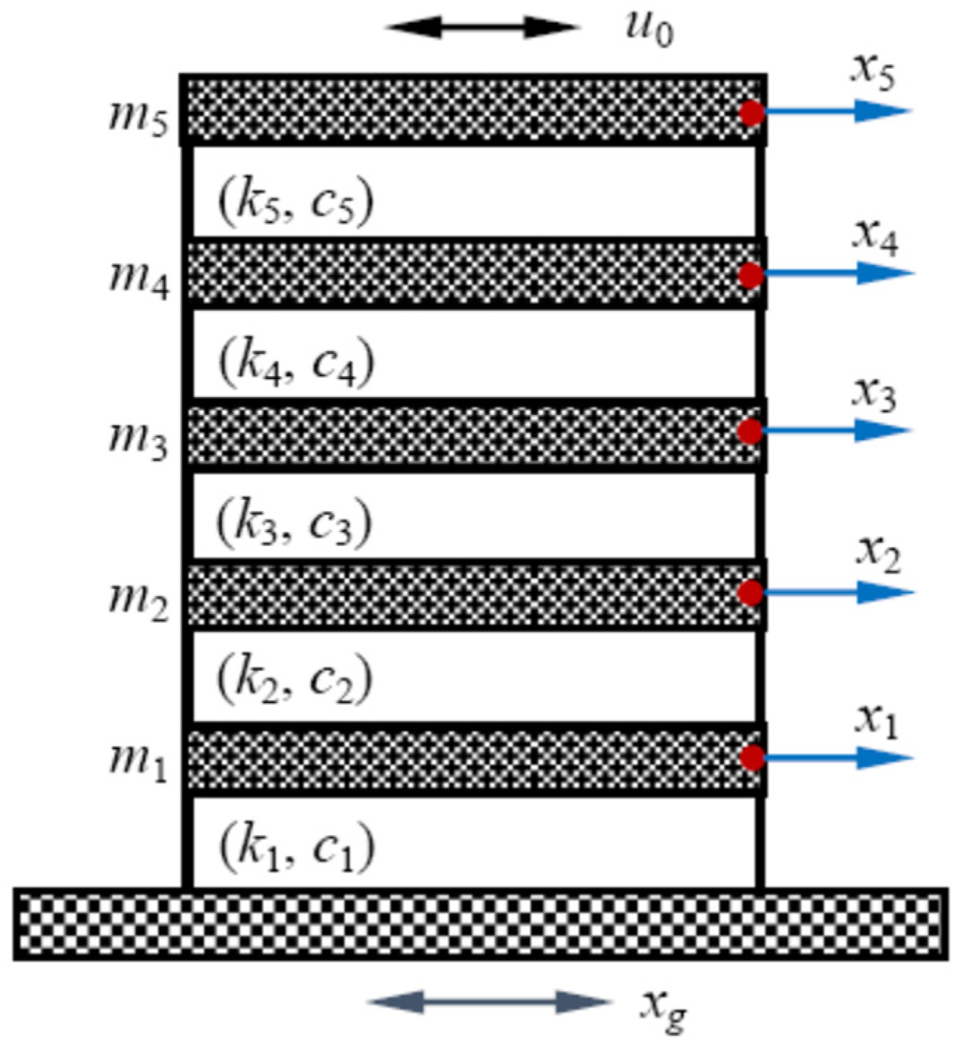
To show the effectiveness of the proposed stochastic optimal control for uncertain systems, consider a five-story frame structure under random base excitation [68], as shown in Figure 1. Horizontal floor displacements (x_i, i = 1, 2, …, 5) relative to the base (x_g) in one direction are considered, and the structure has five degrees of freedom. The ith floor mass, stiffness and damping between the ith and (i − 1)th floors are m_i, k_i and c_i, respectively. The excitation filter can be incorporated in the system, and then the base excitation is regarded as Gaussian white noise. A controller with force u₀ is installed on the top floor. The system equation is expressed in the matrix form as Equation (1), where $F=-{\ddot{x}}_{g}M{I}_e$ and U = u₀, and displacement vector X, mass matrix M, stiffness matrix K, damping matrix C, excitation position vector I_e and control placement matrix B₀ are

$$\begin{gathered} X=\left\{\begin{array}{c}{x}_1\\ x_2\\ \dots \\ x_5\end{array}\right\}, M=\left[\begin{array}{cccc}{m}_1& 0& \dots & 0\\ 0& m_2& \dots & 0\\ \dots & \dots & \dots & \dots \\ 0& 0& 0& m_5\end{array}\right], K=\left[\begin{array}{cccc}{k}_1+k_2& -k_2& \dots & 0\\ -k_2& k_2+k_3& \dots & 0\\ \dots & \dots & \dots & \dots \\ 0& 0& -k_5& k_5\end{array}\right], \\ C=\left[\begin{array}{cccc}{c}_1+c_2& -c_2& \dots & 0\\ -c_2& c_2+c_3& \dots & 0\\ \dots & \dots & \dots & \dots \\ 0& 0& -c_5& c_5\end{array}\right], I_e=\left\{\begin{array}{c}1\\ 1\\ \dots \\ 1\end{array}\right\}, B_0=\left\{\begin{array}{c}0\\ ⋮\\ 0\\ 1\end{array}\right\} \end{gathered}$$

(38)

Rewrite the system equation in the dimensionless form, and then the state equation becomes

$${\displaystyle \frac{\mathrm{d}Z}{\mathrm{d}{t}_0}}=AZ+G(t_0)+Bu$$

(39)

where t₀ is non-dimensional (ND) time, and the ND state vector Z, parameter matrix A, random excitation vector G and control parameter matrix B are

$$Z=\left\{\begin{array}{c}\overline{X}\\ \mathrm{d}\overline{X}/\mathrm{d}{t}_0\end{array}\right\}, A=\left[\begin{array}{cc}0& I\\ -{\overline{M}}^{-1}\overline{K}& -{\overline{M}}^{-1}\overline{C}\end{array}\right], G=f_a\left\{\begin{array}{c}0\\ I_e\end{array}\right\}, B=\left\{\begin{array}{c}0\\ {\overline{M}}^{-1}{B}_0\end{array}\right\}$$

(40)

The ND displacement vector $\overline{X}$, mass matrix $\overline{M}$, stiffness matrix $\overline{K}$ and damping matrix $\overline{C}$ have expressions similar to Equation (38), which has the following elements with the ND time t₀, excitation f_a and control u:

$$\begin{gathered} {\overline{x}}_i={\displaystyle \frac{x_i}{x_0}}, {\overline{m}}_i={\displaystyle \frac{m_i}{m_0}}, {\overline{k}}_i={\displaystyle \frac{k_i}{k_0}}, {\overline{c}}_i={\displaystyle \frac{c_i}{c_0}}, c_0=\sqrt{m_0{k}_0}, \\ {t}_0=t\sqrt{{\displaystyle \frac{k_0}{m_0}}}, f_a={\displaystyle \frac{-m_0{\ddot{x}}_g}{k_0{x}_0}}, u={\displaystyle \frac{u_0}{k_0{x}_0}} \end{gathered}$$

(41)

where x₀, m₀, k₀ and c₀ are constants of displacement, mass, stiffness and damping, respectively. Equation (39) represents an uncertain stochastic control system, where the ND interstory stiffness ${\overline{k}}_i$ and damping ${\overline{c}}_i$ are uncertain parameters to be estimated, samples of the ND random excitation f_a are unknown and the ND control u is to be designed. Only stochastic states Z in a finite time interval with prior mean and intensity of the random excitation are used for optimal estimation and control. The optimal control is calculated by using expression (31) or (34).

In numerical results, the values of the ND parameters are ${\overline{m}}_i=1$, ${\overline{k}}_i=150$ (i = 1, 2), ${\overline{k}}_i=100$ (i = 3, 4, 5), ${\overline{c}}_i=0.9$ (i = 1, 2), ${\overline{c}}_i=0.6$ (i = 3, 4, 5), R_c = 1.0, S_c = diag[S_c1, S_c2], S_c1 = 1.0 × diag[1.0, 1.0, 1.0, 5.0, 20.0] and S_c2 = 1.5 × diag[1.0, 1.0, 1.0, 2.0, 6.0] unless otherwise specified. The ND random excitation f_a = e₀ × f, where e₀ = 5 and f is Gaussian white noise with zero mean and unit intensity. Random earthquake excitation is also considered, finally. According to the proposed stochastic optimal control based on the optimal estimation, the response reduction effectivenesses are obtained and shown in Figure 2, Figure 3, Figure 4, Figure 5, Figure 6, Figure 7, Figure 8, Figure 9, Figure 10 and Figure 11.

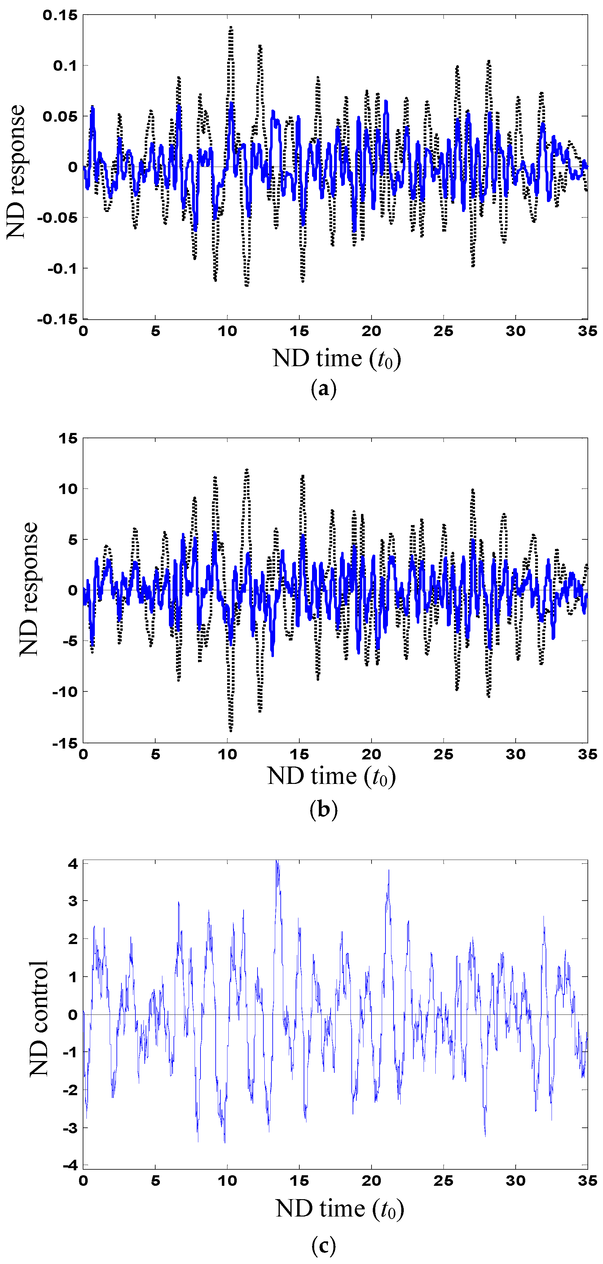
The response reduction of the structural system under white noise excitation is firstly considered. Figure 2 shows the sample of ND random excitation f_a, which is not used for control design and just for illustration. Figure 3a,b shows the ND stochastic responses of uncontrolled and controlled interstory displacements ($\Delta {\overline{x}}_5={\overline{x}}_5-{\overline{x}}_4$) and accelerations on the top floor, respectively, which are used for estimation and control. The estimation accuracy is 1%. The sample of ND control force u is shown in Figure 3c. 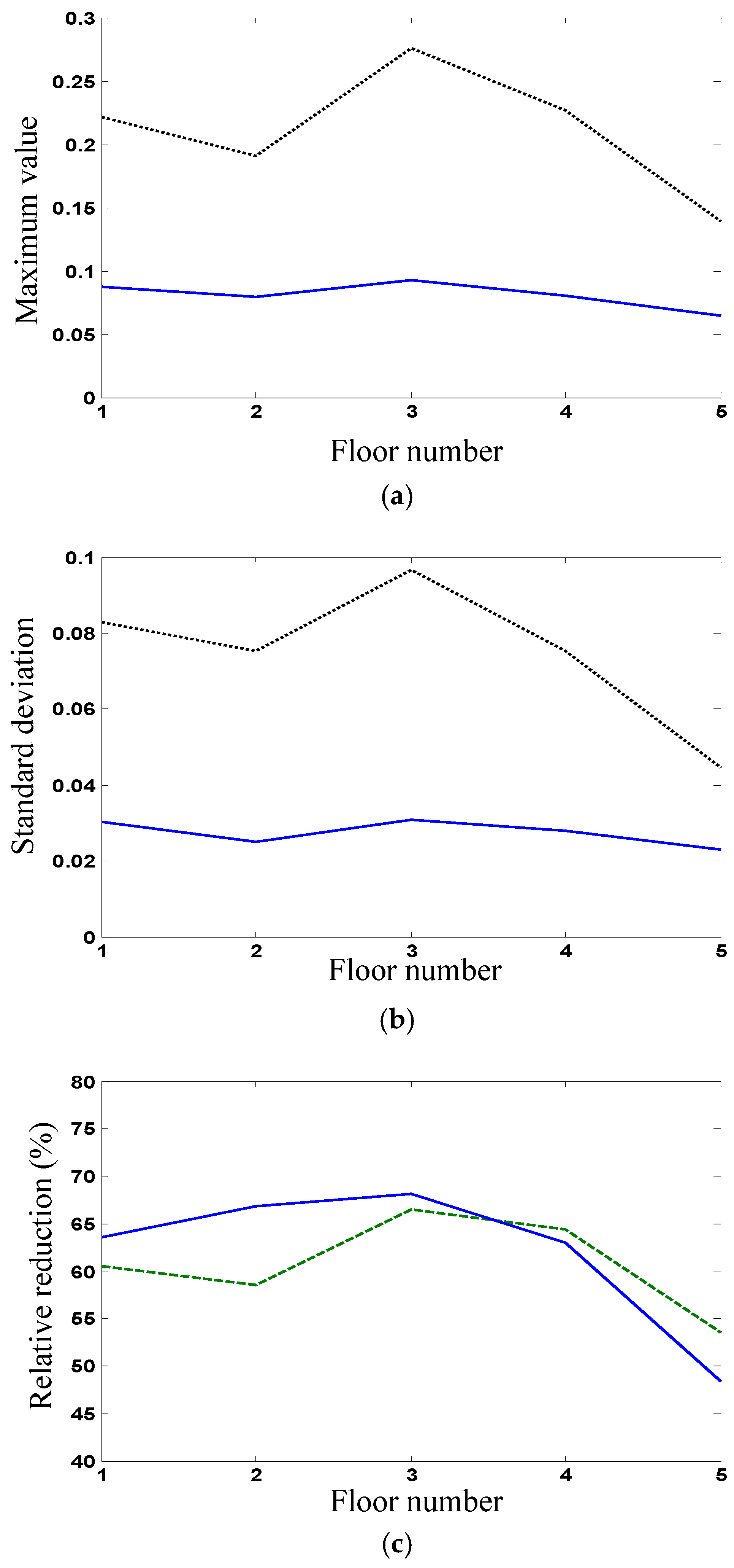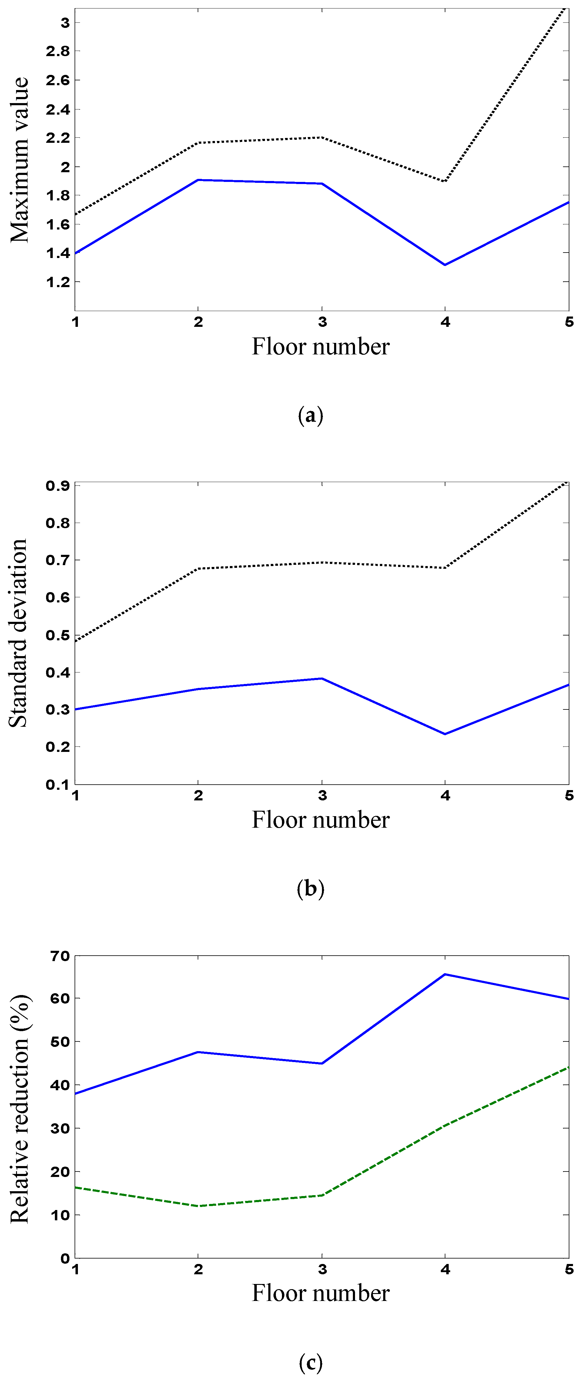Figure 4a,b shows, respectively, the maximum values and standard deviations of uncontrolled and controlled interstory displacements. Figure 4c shows the relative reductions (controlled responses compared with uncontrolled responses) in the maximum values and standard deviations of the interstory displacements. It is seen that the relative reductions (more than 60%) of the first floor are larger than those of the top floor, because the uncontrolled values of the top floor are smaller than those of the first floor. The response reductions of controlled displacements indicate the mitigated structural vibration. For example, the 95% confidence interval of the controlled displacement on the top floor is (−0.045, 0.045). The confidence interval depends greatly on the response standard deviation and will reduce with response. 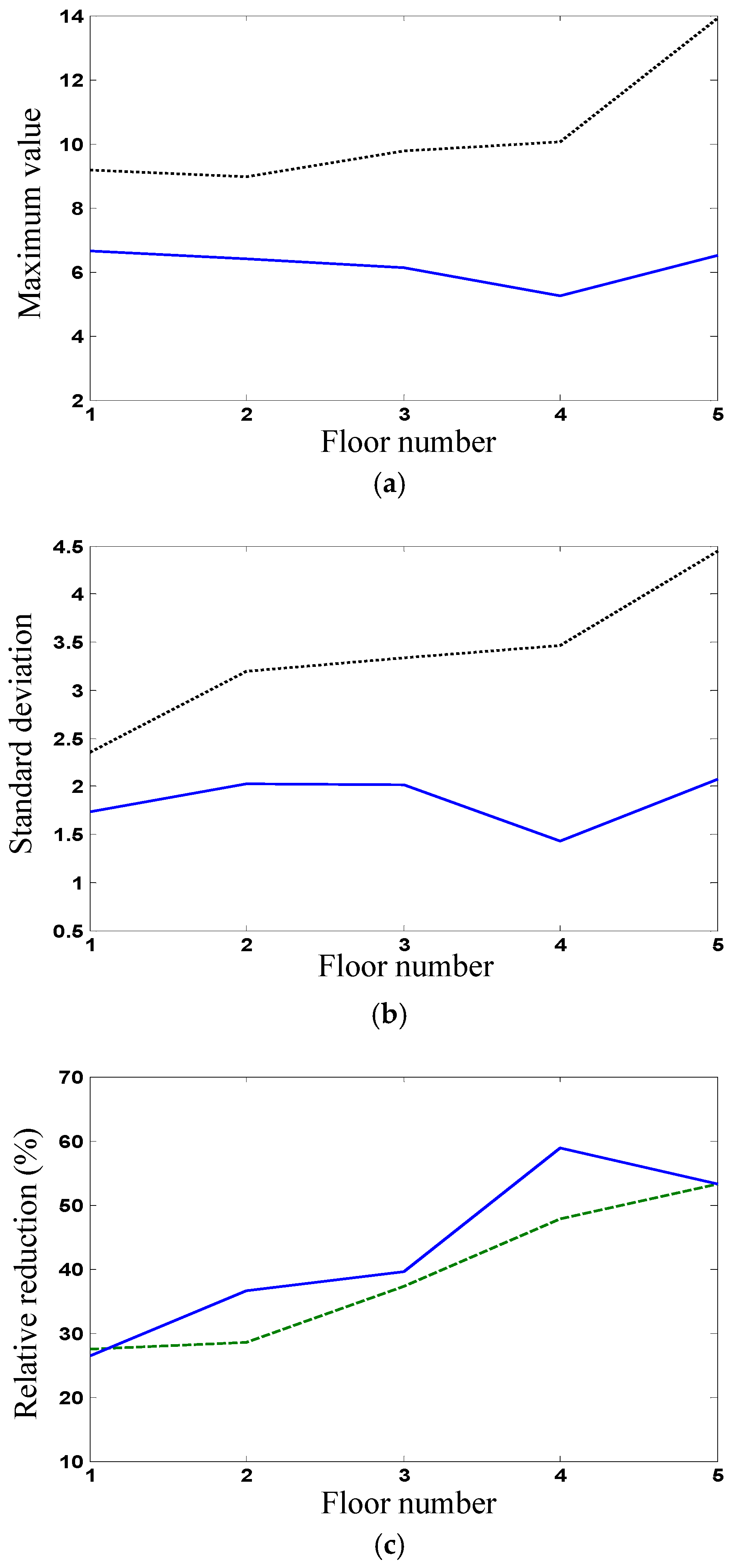Figure 5a,b shows, respectively, the maximum values and standard deviations of uncontrolled and controlled accelerations. Figure 5c shows the relative reductions (controlled responses compared with uncontrolled responses) in the maximum values and standard deviations of the accelerations. The relative reductions (more than 50%) of the top floor are larger than those of the first floor; however, the uncontrolled values of the first floor are smaller than those of the top floor. Thus, the proposed stochastic optimal control for uncertain systems can achieve better control effectiveness for reducing stochastic responses. The relative reductions in the maximum values are close to those in standard deviations, and then only the numerical results on standard deviations of the top floor are given in the following illustration.

5.1. Effects of Estimation Accuracy, Observation Errors and Control Parameters on Control Effectiveness

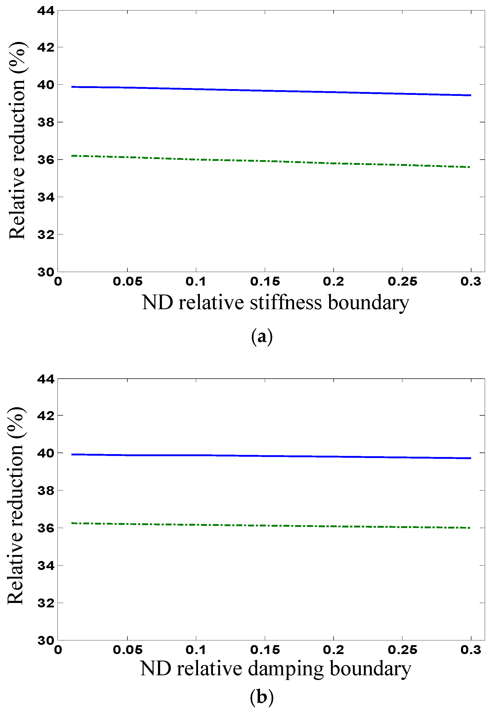
The effects of the estimation accuracy of interstory stiffness and damping, the observation errors of system states in control and the control weight parameters on the control effectiveness are then considered. The uncertain stiffness and damping domains or deviation boundaries ($\Delta {\overline{k}}_i$ and $\Delta {\overline{c}}_i$) increase with the parameter estimation errors. Figure 6a shows the relative reductions in the standard deviations of the interstory displacements ($\Delta {\overline{x}}_5$) and accelerations on the top floor per unit control force in standard deviation for different stiffness boundaries ($\Delta {\overline{k}}_5/{\overline{k}}_5$). Figure 6b shows the relative reductions in the standard deviations of the interstory displacements ($\Delta {\overline{x}}_5$) and accelerations on the top floor per unit control force in standard deviation for different damping boundaries ($\Delta {\overline{c}}_5/{\overline{c}}_5$). It is seen that all the relative reductions decrease with increasing the deviation boundaries slightly and, thus, the proposed stochastic optimal control for uncertain systems is robust.

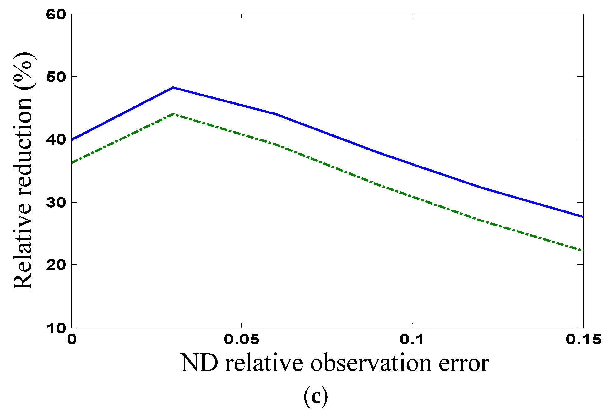
Figure 6c shows the relative reductions in the standard deviations of the interstory displacements ($\Delta {\overline{x}}_5$) and accelerations on the top floor per unit control force in standard deviation for different relative observation errors of the displacement on the top floor (${\overline{x}}_{e5}/{\overline{x}}_5$). It is seen that both relative reductions remarkably decrease with increasing observation errors that become larger than certain values (e.g., 3%). Thus, the observation errors of system states for the optimal control need to be controlled in certain small domains. 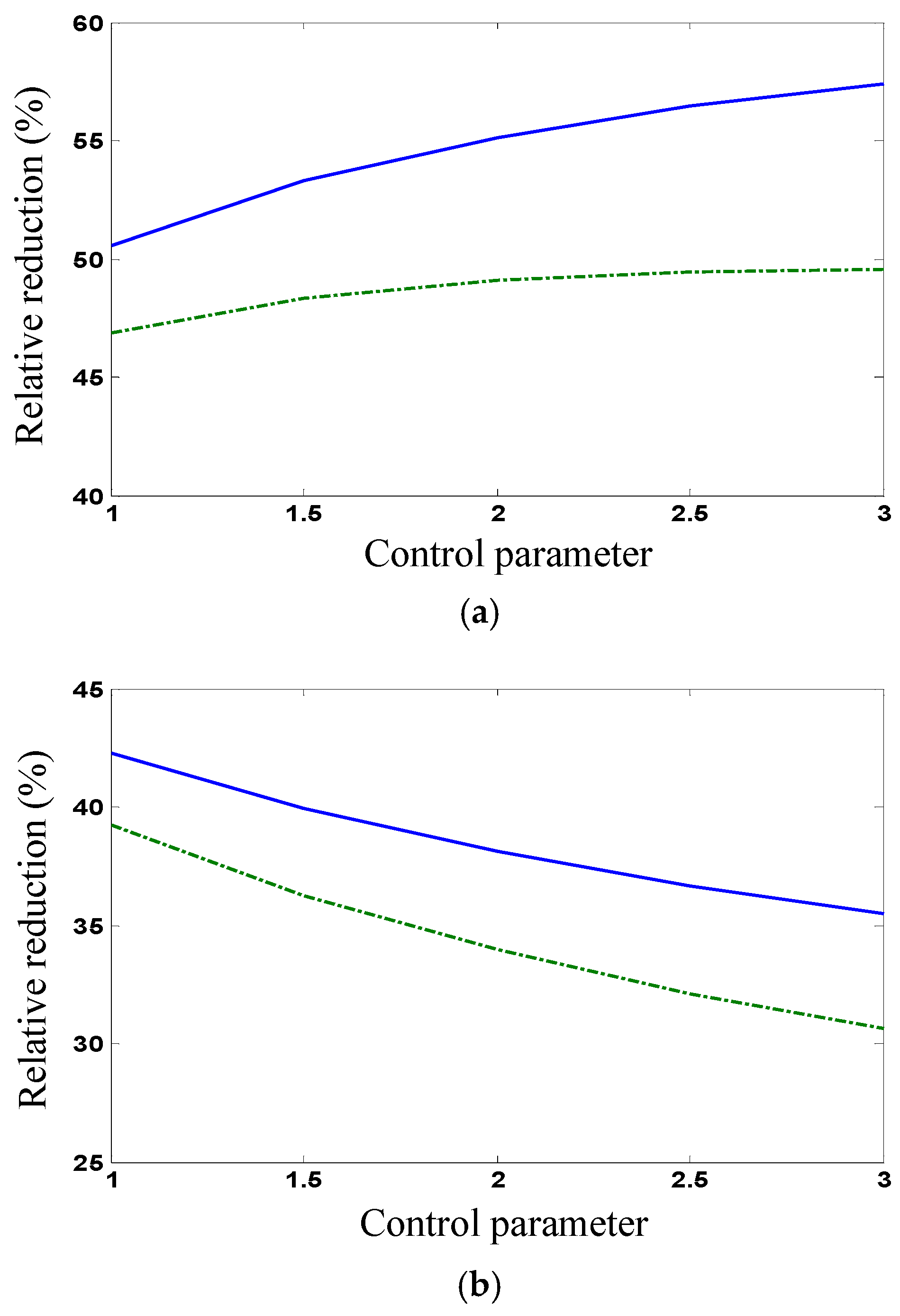Figure 7a,b shows the relative reductions in the standard deviations of the interstory displacements ($\Delta {\overline{x}}_5$) and accelerations on the top floor and those per unit control force in standard deviation for different control weight parameters (s_c2, S_c2 = s_c2 × diag[1.0, 1.0, 1.0, 2.0, 6.0]), respectively. It is seen that the relative reductions or control effectiveness can be improved by increasing the control weight parameters (Figure 7a); however, the relative reductions per unit control force or control efficiency will decrease correspondingly (Figure 7b).

5.2. Control Effectiveness for Uncertain Structure Under Earthquake Excitation

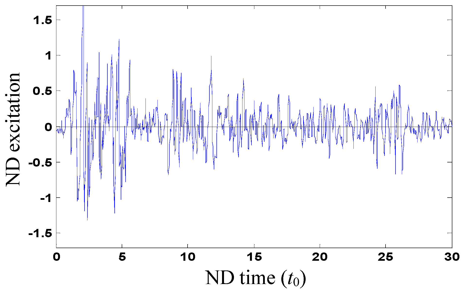
The proposed stochastic optimal control for the structural system under random earthquake excitation is also considered. The acceleration record of the El Centro earthquake is used as the random excitation, which approximates a filtering Gaussian white noise, and the prior statistics errors have a slight effect on the parameter estimation [1,68]. Figure 8 shows the sample of ND random excitation (f_a). 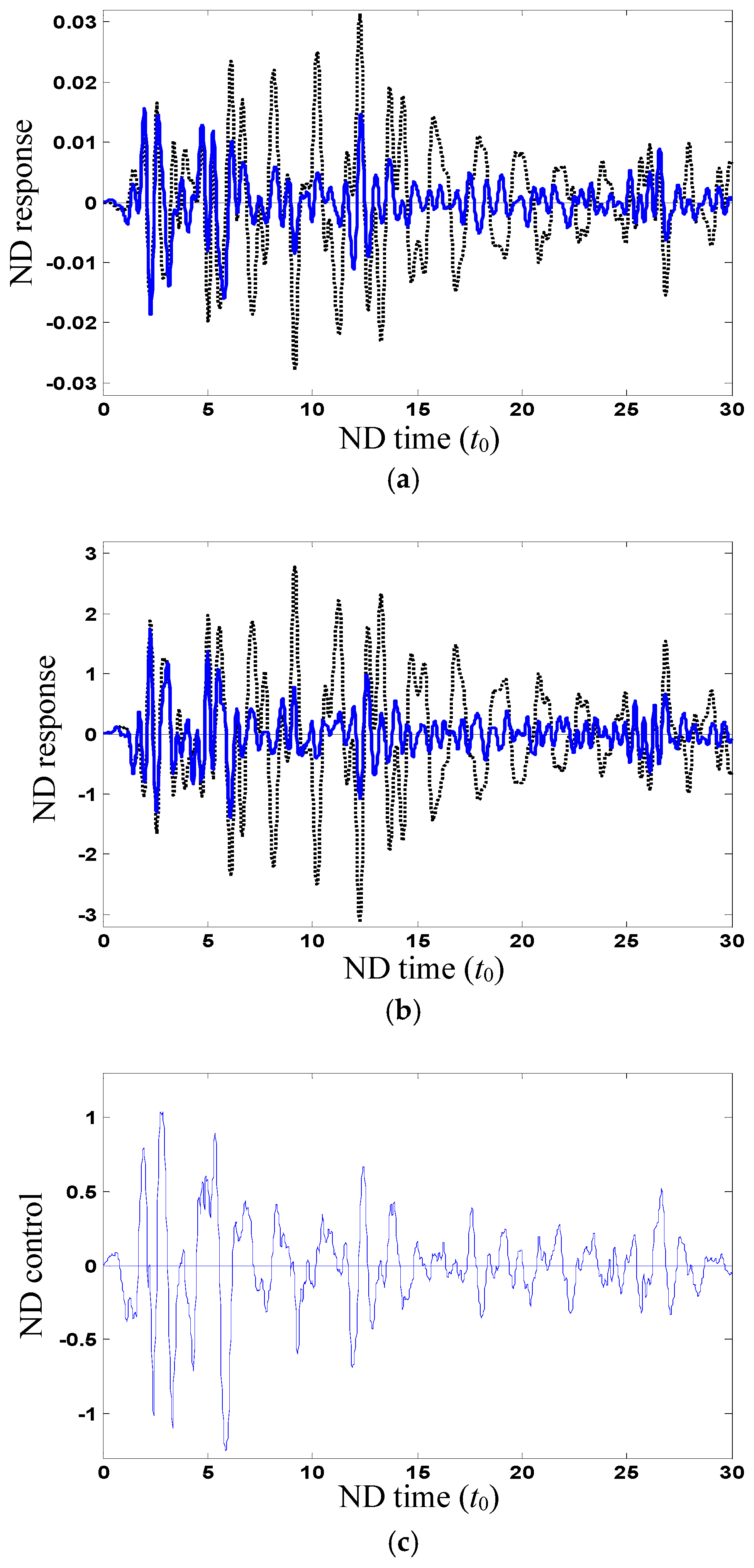Figure 9a,b shows the ND stochastic responses of uncontrolled and controlled interstory displacements ($\Delta {\overline{x}}_5$) and accelerations on the top floor, respectively, where the control weight parameters S_c2 = 3.5 × diag[1.0, 3.0, 1.0, 2.0, 6.0] and the estimation accuracy is 1%. The sample of ND control force u is shown in Figure 9c. 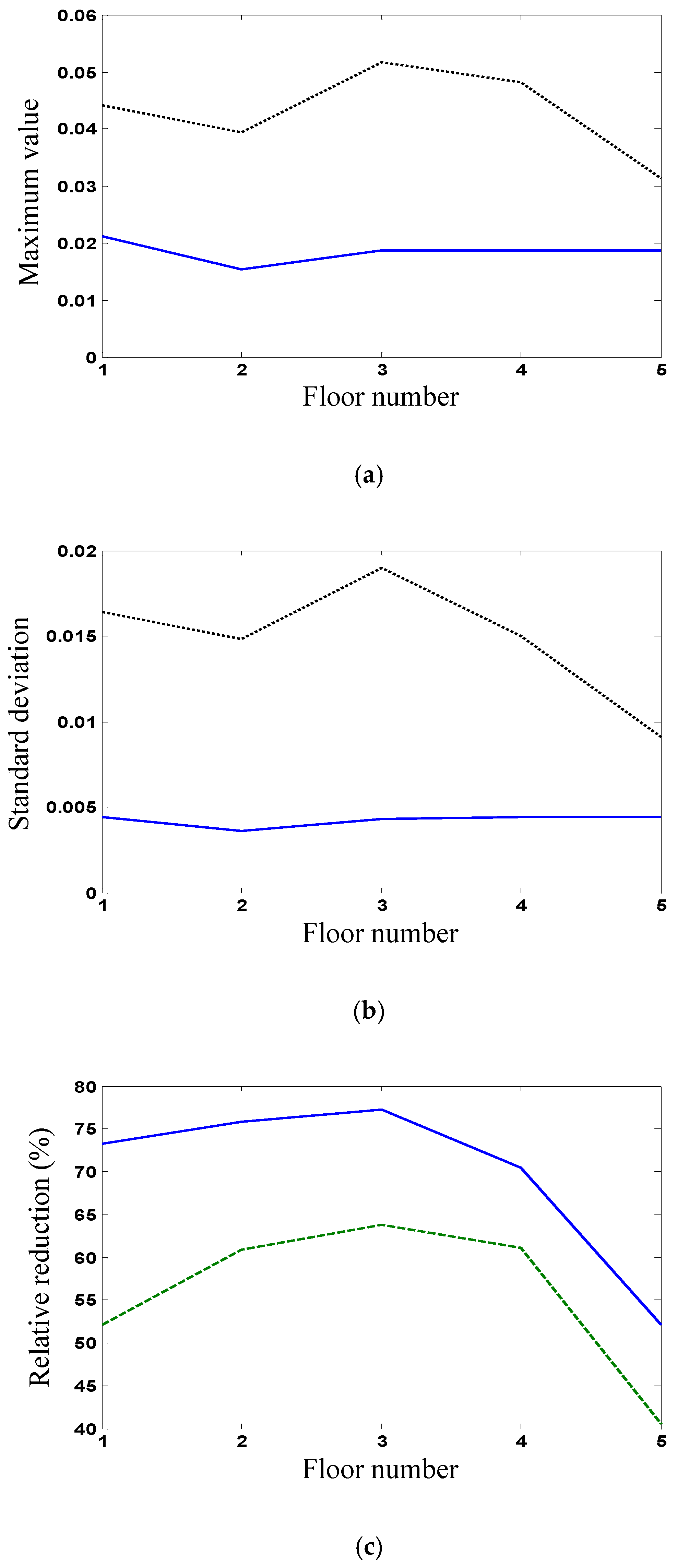Figure 10a,b shows, respectively, the maximum values and standard deviations of uncontrolled and controlled interstory displacements. Figure 10c shows the relative reductions (controlled responses compared with uncontrolled responses) in the maximum values and standard deviations of the interstory displacements. It is seen that the relative reductions (more than 50% for the maximum value and 70% for the standard deviation) of the first floor are larger than those of the top floor; however, the uncontrolled values of the top floor are smaller than those of the first floor. Figure 11a,b shows, respectively, the maximum values and standard deviations of uncontrolled and controlled accelerations. Figure 11c shows the relative reductions (controlled responses compared with uncontrolled responses) in the maximum values and standard deviations of the accelerations. The relative reductions (more than 40% for the maximum value and 60% for the standard deviation) of the top floor are larger than those of the first floor, but the uncontrolled values of the first floor are smaller than those of the top floor. Thus, the proposed stochastic optimal control for uncertain systems under earthquake excitations can also achieve better control effectiveness for reducing stochastic responses.

Based on the above numerical results, it is obtained that by using the proposed control strategy, the relative reductions in the maximum values and standard deviations of the ND interstory displacements of the first floor are more than 60%. Although they are larger than those of the top floor, the uncontrolled values of the top floor are smaller than those of the first floor. The relative reductions in the maximum values and standard deviations of the ND accelerations of the top floor are more than 50%. However, the uncontrolled values of the first floor are smaller than those of the top floor. Thus, the proposed stochastic optimal control for uncertain systems can achieve better control effectiveness for reducing stochastic responses to white noise excitation. The relative reductions decrease with increasing the deviation boundaries slightly and, thus, the proposed stochastic optimal control for uncertain systems is robust. The relative reductions remarkably decrease with increasing state observation errors that are larger than certain values and, thus, the observation errors of system states for the optimal control need to be controlled in certain small domains. The relative reductions or control effectiveness can be improved further by optimizing the control weight parameters; however, the relative reductions per unit control force or control efficiency may change differently. For uncertain systems under earthquake excitation, the proposed stochastic optimal control can also achieve better control effectiveness for reducing stochastic responses. For example, the relative reductions in the ND interstory displacements of the first floor are more than 50% for the maximum value and 70% for the standard deviation. The relative reductions of the ND accelerations of the top floor are more than 40% for the maximum value and 60% for the standard deviation.

6. Discussion

The proposed stochastic optimal control strategy for uncertain structural systems under random excitations includes two parts: Bayes optimal parameter estimation and optimal state control based on minimax stochastic dynamical programming. For the estimation, the posterior probability density conditional on observation states expressed using the likelihood function conditional on system parameters according to Bayes’ theorem or the logarithmic posterior expressed using the geometrically averaged likelihood do not have any limitations on probability distributions. The differential Equation (15) for state means does not have any limitations on stochastic processes. The differential Equations (16) and (17) for state covariances are derived from systems under white noise excitation and, however, can be extended to non-white noise excitations based on stochastic dynamics theory. The conditional statistics (20) and (21) obtained based on the optimal state estimation are usable for general stochastic processes. Thus, the Bayes optimal estimation method is applicable to general stochastic processes under the extended differential equations for state covariances. For the control, the minimax strategy, designed by minimizing the performance index for the worst-parameter system, which is obtained by maximizing the performance index based on game theory, does not have any limitations on stochastic processes. Different from the conventional non-optimal robust control, it uses game theory to combine robustness and optimization. The minimax dynamical programming Equation (28) is derived from systems under white noise excitation and, however, can be extended to non-white noise excitations based on the minimax stochastic dynamical programming principle. The application of the Ito differential rule and its results have some changes. The worst parameters determined by maximization of the equation and the optimal control determined by minimization of the resulting equation have certain variations, accordingly. Thus, the minimax stochastic optimal control strategy is applicable to general stochastic processes under the extended dynamical programming equation. Many practical excitations can be represented by filtering Gaussian white noises. By incorporating the filter in the system, the augmented system will be subjected to white noise excitations, and then the above proposed stochastic optimal control strategy for uncertain structural systems can be applied directly. However, for the other random excitations and state processes, the proposed stochastic optimal control strategy needs to be extended, for example, including the differential equations for state covariances and the dynamical programming equation. If the state observation noises are considered, the optimal control becomes a partially observable stochastic optimal control problem. After state filtering, such as Kalman filtering or its extended filtering, the proposed stochastic optimal control strategy for uncertain structural systems is still applicable. For other control objectives, such as reliability and stability, the performance index (26) needs to be modified, and the dynamical programming equation is extended accordingly. Then, the proposed stochastic optimal control strategy for uncertain structural systems is applicable.

7. Conclusions

A stochastic optimal control strategy for uncertain structural systems under random excitations is proposed, based on the minimax stochastic dynamical programming principle and the Bayes optimal estimation method with the combination of stochastic dynamics and Bayes inference. The proposed optimal control mainly includes two parts: optimal parameter estimation and mimimax dynamical programming. The optimal estimation based on stochastic dynamics and optimal state estimation estimates uncertain parameters more reliably and accurately, and then the obtained parameter domains are smaller. The optimal control based on minimax stochastic dynamical programming has the control law determined as more effective and robust. The proposed stochastic optimal control based on Bayes optimal estimation depends only on observed states and is a new development of the optimal control for uncertain systems under random excitations.

Numerical results for a five-story frame structure under random base excitations demonstrate that (1) the proposed optimal control for an uncertain structure under white noise and earthquake excitations can achieve better control effectiveness; (2) the control effectiveness is robust about uncertain parameters and estimation errors; and (3) the control effectiveness can decrease when the state observation errors are larger, and then the observation accuracy is important. The proposed stochastic optimal control strategy based on Bayes optimal estimation is extendable to solve other control problems, including the partially observable control, semiactive control, reliability and stability control of uncertain stochastic systems.