Study on the Impact of Combined Action of Temperature Differential and Freeze–Thaw Cycle on the Durability of Cement Concrete

Abstract

As a primary construction material, concrete plays a vital role in the development of infrastructure, including bridges, highways, and large-scale buildings. In Northeast China, the structural integrity of concrete faces severe challenges due to freeze–thaw cycles and substantial diurnal temperature variations. This study involved a thorough examination of concrete’s performance under varying numbers of temperature differential cycling (60 to 300) and freeze–thaw cycles (75 to 300). The results showed that both freeze–thaw and temperature differential cycling led to increasing mass loss with the number of cycles. Peak mass losses reached 3.1% and 1.2% under freeze–thaw and temperature differential cycles, respectively, while the combined action resulted in a maximum mass loss of 4.1%. The variation trends in dynamic elastic modulus and compressive strength differed depending on the environmental conditions. Under identical freeze–thaw cycling, both properties exhibited an initial increase followed by a decrease with increasing temperature differential cycles. After 120 temperature differential cycles, the dynamic modulus and compressive strength increased by 4.7–6.2% and 7.5–10.9%, respectively. These values returned to near their initial levels after 180 cycles and further decreased to reductions of 17.0–22.6% and 15.3–29.4% by the 300th cycle. In contrast, under constant temperature differential cycles, dynamic modulus and compressive strength showed a continuous decline with increasing freeze–thaw cycles, reaching maximum reductions of 5.0–11.5% and 18.1–31.8%, respectively. Notably, the combined effect of temperature differential and freeze–thaw cycles was significantly greater than the sum of their individual effects. Compared to the superposition of separate effects, the combined action amplified the losses in dynamic modulus and compressive strength by factors of up to 3.7 and 1.8, respectively. Additionally, the fatigue life of concrete subjected to combined temperature differential and freeze–thaw cycles followed a two-parameter Weibull distribution. Analysis of the S-N_f curves revealed that the coupled environmental effects significantly accelerated the deterioration of fatigue performance.

1. Introduction

Due to its excellent compressive strength, remarkable durability, and economic efficiency, cement concrete has gradually emerged as one of the most commonly utilized materials in the construction of highways, bridges, and various infrastructure projects. Its performance is directly linked to the safety, durability, and economic benefits of buildings. Nevertheless, in real-world engineering conditions, especially in the northeastern regions of China, cement concrete faces the dual challenges of temperature differential cycling and freeze–thaw cycling. It is widely recognized that freeze–thaw cycles are among the primary factors compromising the durability of cement concrete structures in cold climates. This process, by altering the state of water in the concrete’s pores and causing changes in the volume of pore water, generates internal stresses, subsequently deteriorating the concrete’s performance. Additionally, due to the various components within concrete and their differing thermal properties, uneven deformation under temperature cycles leads to the generation of thermal stresses and the formation and development of internal microcracks, adversely affecting the concrete’s performance. Such effects are particularly pronounced in regions with large diurnal temperature fluctuations, where the impact on the long-term durability of concrete structures becomes even more critical. Although numerous studies have investigated the effects of either freeze–thaw cycling or temperature differential cycling on concrete performance, systematic research on their combined action remains limited. In practice, these two environmental factors often occur simultaneously, and their coupling may lead to more complex and severe damage mechanisms. Therefore, understanding the performance evolution of concrete under the combined effects of temperature differential and freeze–thaw cycles is of critical importance for improving the durability of structures operating in extreme climatic conditions.

Extensive research, both domestically and internationally, has been conducted on the durability of concrete under freeze–thaw cycles. Beginning in the 1940s, numerous hypotheses, such as hydrostatic pressure theory and osmotic pressure theory, have been proposed to elucidate the underlying mechanisms responsible for freeze–thaw-induced deterioration [1,2,3,4,5,6,7]. Shi [8] examined how freeze–thaw cycles influence the mechanical properties of concrete, concluding that compressive strength, tensile strength, shear strength, and elastic modulus all degrade to varying degrees with increased freeze–thaw cycling. Additionally, Shang et al. [9,10], through experimental investigations, observed significant reductions in concrete’s uniaxial compressive and tensile strengths post freeze–thaw cycling, accompanied by increases in peak strain on the stress–strain curves and notable declines in deformation modulus. Cho [11] studied the relationships among key parameters of cement concrete (such as water–cement ratio, air content, and number of freeze–thaw cycles) and proposed a new prediction method—the Response Surface Method (RSM)—to predict the cumulative damage of cement concrete under the freeze–thaw cycle, which was validated through experiments. Vesikarr et al. [12] investigated the relationship between freeze–thaw damage in concrete and the frequency of rapid freeze–thaw cycles, subsequently developing a predictive equation for estimating the service life of concrete structures subjected to a predetermined number of freeze–thaw cycles. Guan et al. [13,14] proposed a universal multivariate model for predicting the fatigue life of cement concrete under different boundary conditions and single- or multiple-factor compound actions, which was validated through rapid freeze–thaw tests and combined action tests of ammonium sulfate and freeze–thaw cycles. Ou et al. [15] conducted research on the fatigue life and associated characteristics of concrete beams under varying degrees of freeze–thaw deterioration. Their findings demonstrated that the flexural fatigue life can be accurately characterized by a Weibull distribution, with reliability decreasing significantly as the freeze–thaw cycles accumulate. Boyd et al. [16] investigated the fatigue life of concrete with varying degrees of freeze–thaw damage. Their findings revealed that freeze–thaw damage led to a certain level of degradation in the fatigue performance of concrete. However, during the early stages of damage, the freeze–thaw cycles had little impact on the ultimate tensile load capacity of the concrete. H. Kuosa et al. [17] studied the degradation mechanisms of concrete under the combined effects of freeze–thaw cycling, carbonation, and chloride ion penetration. The results indicated that freeze–thaw damage can increase the carbonation depth and exacerbate chloride ion migration in concretes with higher water–cement ratios, thereby reducing the overall service life of the material. In summary, existing research shows that freeze–thaw cycles have a significant deteriorating effect on the mechanical properties of concrete; hence, the study of concrete’s frost resistance is of utmost importance.

In recent years, increasing research interest has focused on the impact of temperature differential cycling on concrete performance. Al-Tayyib et al. [18] examined the durability of cement concrete exposed to repeated temperature differentials ranging from ambient temperature to 80 °C over a total of 90 cycles. Their results demonstrated that, after completing 90 cycles, compressive and flexural strengths were reduced by nearly 30%, with the greatest rate of strength loss occurring around cycle 30. Kanellopoulos et al. [19] observed that the mechanical properties of cement concrete improved significantly after 30 temperature cycles (20 °C to 90 °C) but declined after 90 cycles. Research by Shokrieh et al. [20] showed that optimized polymer cement concrete experienced a reduction of 4.9% in compressive strength and 17.4% in flexural strength after undergoing Temperature Differential Cycling II (25 °C to 70 °C), while Temperature Differential Cycling I (25 °C to −30 °C) and Temperature Differential Cycling III (−30 °C to 70 °C) had no significant impact on strength. Heidari-Rarani et al. [21] examined the influence of different temperature differential cycles (25–30 °C, 25–70 °C, and 30–70 °C) on the mechanical characteristics of resin cement concrete. Their results indicated substantial reductions in both tensile strength and fracture toughness under temperature differential cycling, with further deterioration occurring as the average cycling temperature increased. Huang et al. [22] investigated how alterations in the microstructure of the cement matrix and interfacial transition zone caused by thermal cycling relate to the mechanical behavior of concrete, and developed a micromechanical model incorporating porosity and microcrack parameters. Xiao et al. [23] studied the changes in mechanical properties and microstructural damage of different concretes (C25, C40) after thermal fatigue, finding that the degree of deterioration of concrete under thermal fatigue was significant, and the extent of strength degradation increased with the temperature difference (20 °C, 30 °C, 40 °C) and number of temperature differential cycles. These studies demonstrate that temperature differential cycling significantly deteriorates the performance of concrete; hence, considering the impact of temperature differential cycling is crucial in enhancing the design precision and durability of concrete structures in regions with large diurnal temperature differences, such as Northeast and Northwest China.

Furthermore, fatigue behavior has consistently been a central research focus within concrete durability studies. Byung [24] carried out statistical analyses on the fatigue life of concrete beams under variable amplitude loading, concluding that the fatigue life distribution closely fits a two-parameter Weibull model. Zhou et al. [25] studied the axial compression fatigue strength of concrete after high-temperature treatment, finding that after being subjected to 200 °C, the axial compression fatigue strength of concrete decreased by about 28% compared to its normal temperature state, and the axial compression fatigue strength of the high-temperature-treated concrete was more significantly affected by the number of fatigue load cycles. Zhao et al. [26] investigated the effects of different high-temperature regimes (varying temperatures, varying constant temperature durations) on the performance of high-strength concrete. They found that with the increase in heating temperature and constant temperature duration, the compressive strength, modulus elasticity, and mass of high-strength concrete generally showed a downward trend, with the heating temperature having a more significant impact on the deterioration of the mechanical properties of high-strength concrete. Xue et al. [27] performed a reliability assessment on the compressive fatigue life of slag powder concrete exposed to freeze–thaw cycles. They proposed a compressive fatigue life prediction model utilizing equivalent damage theory. Zhu et al. [28] investigated the flexural fatigue life distribution characteristics of self-compacting concrete after freeze–thaw cycles. Their findings demonstrated that fatigue life data align closely with a two-parameter Weibull distribution, with increased dispersion observed as the number of freeze–thaw cycles rose, but a decreasing trend was noted with higher stress levels. These studies indicate that in the research on concrete fatigue performance, scholars primarily focus on the impact of fixed factors such as constant mechanical loads, seismic action [29], or temperatures. Consideration of variable factors is less common, with the majority of research concentrating on exploring the effects of freeze–thaw cycles. However, as a form of temperature variation, temperature cycles and their impact on the fatigue performance of concrete also warrant in-depth investigation.

In summary, current research on the durability of concrete has primarily focused on exploring the effects of freeze–thaw cycles, fixed temperatures, or temperature histories, with less emphasis on the combined effects of temperature differential cycling and freeze–thaw cycles. In reality, within engineering environments, daily diurnal temperature variations leading to temperature differential cycling and seasonal freeze–thaw cycling often coexist. Neglecting such coupled environmental actions may lead to premature damage within the designed service life of structures, or result in significant economic losses and safety risks due to insufficient preventive measures [30]. Therefore, investigating the combined influence of temperature differential and freeze–thaw cycling on concrete durability is of great significance—not only from a theoretical standpoint, but also for the practical optimization of cement concrete materials and durability design in engineering applications. Therefore, studying the combined effects of temperature differential cycling and freeze–thaw cycling on the durability of concrete is not only of significant theoretical relevance, but also provides practical guidance for the optimization of performance and durability design of cement concrete materials in actual engineering applications.

This study specifically evaluates the combined effects of temperature differential cycling and freeze–thaw conditions on the mechanical properties of C40-grade cement concrete. Its objective is to deepen the current understanding and enhance concrete performance under severe environmental conditions. Through comprehensive experimental design, this research investigates cement concrete subjected to various temperature differential cycling (60 to 300 cycles, with tests conducted after every 60 cycles) and subsequent freeze–thaw cycling (75 to 200 cycles, with tests conducted after every 75 cycles). The research encompasses statistical and analytical assessments of mass, dynamic elastic modulus, compressive strength, and compressive fatigue life. This research aims to summarize the patterns of impact caused by the combined effects of temperature cycles and freeze–thaw cycles on cement concrete performance, revealing the mechanism of their interaction. The results obtained are expected to provide critical insights into improving concrete frost resistance within complex environmental contexts, as well as offer theoretical guidance for optimizing material performance in engineering practice.

2. Experimental Materials and Methods

2.1. Experimental Materials

The primary raw materials selected for the concrete tests include cement, Class II fly ash, S95-grade mineral powder, medium sand, continuously graded crushed stone (5–20 mm), Subote-brand polycarboxylate superplasticizer, an air-entraining agent, and water. The selection of these materials was based on their specific performance characteristics. In particular, Jidong-brand P·O 42.5 ordinary Portland cement was employed owing to its exceptional early-age strength and durability, making it particularly suitable for high-strength concrete. The key physical and mechanical properties of the cement used in this study are summarized in

Table 1. Key physical and mechanical characteristics of the cement employed in the experimental study.

Specific Surface Area [m2/kg]	Setting Time [min]		Flexural Strength [MPa]		Compressive Strength [MPa]
	Initial Setting	Final Setting	3 d	28 d	3 d	28 d
372	217	280	4.5	7.3	22.4	48.5

.

Aggregates: Natural river sand and crushed stone with a reasonable particle size distribution are used. River sand is employed as fine aggregate, while crushed stone serves as coarse aggregate, ensuring the stability and uniformity of the concrete.

Air entraining agent: Adding air entraining agent to enhance the frost resistance of concrete. SJ-2 air entraining agent is selected, with a dosage of 0.01% by weight of cement and an overall air content of 4.5%

The concrete mix proportion design is carried out in accordance with JGJ55-2011 “Ordinary Concrete Mix Proportion Design Regulations” [31] to determine the quantities of each raw material. The design strength grade of the concrete is C40, with a slump of 220 mm. The specific mix proportion used for the experiment is presented in

Table 2. Experimental concrete mix proportion (kg/m³).

Cement	Fly Ash	Mineral Powder	Medium Sand	Crushed Stone	Water	Water-Reducing Agent	Air Entraining Agent
410	30	30	786	1000	174	9.3	0.041

.

The preparation and curing of the concrete specimens followed the standard procedure specified in GB/T 50081-2019, “Standard for Test Methods of Physical and Mechanical Properties of Concrete” [32]. A standard concrete mixer was utilized to achieve homogeneous mixing. Additionally, a vibrating table was utilized to compact the specimens, ensuring the density of the concrete structure. After 24 h of specimen preparation, demolding was carried out. Following demolding, the concrete specimens were cured in a standard curing chamber (maintained at 20 °C ± 2 °C and relative humidity above 95%) for 35 days before testing commenced (for reference, the international standard ASTM C511 specifies a curing temperature of 23 °C ± 2 °C with a relative humidity of at least 95%).

The specimen dimensions and quantities adhered to GB/T 50081-2019 “Standard for Test Methods of Physical and Mechanical Properties of Concrete” [32] and GB/T 50082-2009 “Standard for Test Methods of Physical and Mechanical Properties of Concrete” [33]. Prism specimens measuring 100 mm × 100 mm × 400 mm were employed to evaluate mass changes and dynamic modulus of elasticity. Cube specimens measuring 100 mm × 100 mm × 100 mm were prepared for compressive strength and compressive fatigue life tests (it is worth noting that ASTM C39 specifies standard specimens for compressive strength as cylinders with a diameter of 150 mm and a height of 300 mm, while ASTM C666 recommends prisms of 76 mm × 76 mm × 406 mm for freeze–thaw testing). For each temperature differential cycling scenario (0, 60, 120, 180, 240, and 300 cycles), 63 specimens were fabricated. Specifically, 3 specimens served as references for mass and dynamic modulus testing; 15 specimens (3 per cycle count) were tested for compressive strength after varying freeze–thaw cycle counts (0, 75, 150, and 200 cycles); and 45 specimens were utilized to determine compressive fatigue life, with 9 specimens per freeze–thaw cycle count (3 specimens per stress level).

Table 3. Quantity of specimens used in the experiment.

Experiment	Times of Temperature Differential Cycling Tj	Number of Freeze–Thaw Cycle Fi					Sub Total	Total
		0	75	150	225	300
Mass dynamic modulus of elasticity	Tj (i = 0, 60, 120, 180, 240, 300)	3					3	63
Compressive strength		3	3	3	3	3	15
Compressive fatigue life		9	9	9	9	9	45
Total								378

details the specimen quantities employed in this investigation.

2.2. Experimental Method

2.2.1. Temperature Differential Cycling Test

Typical regions in Northeast China, including Genhe in Inner Mongolia and Beian, Harbin, and Mudanjiang in Heilongjiang Province, are characterized by a temperate monsoon climate and flat terrain. During summer, extended daylight hours and intense solar radiation cause significant pavement surface heating. At night, the relative humidity is low and thermal retention is poor. Moreover, the absence of mountain barriers allows cold Siberian air to descend rapidly to the ground surface, resulting in a rapid drop in pavement temperature. As a result, the diurnal temperature difference on cement concrete pavements can exceed 30 °C. Based on these environmental conditions, the temperature range for thermal cycling in this study was set from 20 °C to 60 °C to better replicate the actual climate characteristics of Northeast China. The temperature differential cycling tests were performed using an alternating high- and low-temperature chamber manufactured by Shanghai Yi Hua Instrument Equipment Co., Ltd., Shanghai, China. The temperature range for the temperature cycle was set from 20 °C to 60 °C, with both the heating and cooling rates set at 2 °C/min. After each heating (or cooling) to the target temperature, the specimens were kept at a constant temperature for 160 min, allowing the center and surface temperatures of the specimens to equalize, thereby eliminating the impact of thermal stress on subsequent test results. Similarly, before initiating the temperature cycle, all specimens were first placed in a constant temperature environment of 20 °C for 240 min to ensure uniformity of the surface and center temperatures of the specimens at the initial state. The mechanism of temperature differential cycling for this experiment was set as follows:

(1)

Heating the temperature control chamber to 60 °C, with a heating rate of 2 °C/min;

(2)

Setting the temperature control chamber to a constant temperature of 60 °C and placing the specimens in the chamber for 160 min;

(3)

Cooling the temperature control chamber to 20 °C, with a cooling rate of 2 °C/min;

(4)

Setting the temperature control chamber to a constant temperature of 20 °C and placing the specimens for 160 min;

Steps (1) to (4) were repeated for one complete temperature cycle. Each cycle lasted for a total of 360 min.

The principle and procedure of temperature differential cycling are illustrated in Figure 1. To achieve a more accurate evaluation of the effects of temperature differential cycling on specimen performance and improve the efficiency of the experimental process, systematic testing protocols were implemented. In this study, research was conducted within the range of 0 to 300 temperature cycles. Additionally, after every 60 cycles, 63 specimens were removed from the temperature control chamber to continue with the freeze–thaw cycle test.

2.2.2. Freeze–Thaw Cycle Test

This study utilized the “Rapid Freezing Method” for the freeze–thaw cycle test, designed according to GB/T 50082-2009 “Standard for Test Methods of Physical and Mechanical Properties of Concrete” [33]. The main steps are as follows:

(1)

Immerse the specimens in water at 20 ± 2 °C for 4 days and then remove, wipe off surface moisture, and check external dimensions (in comparison, ASTM C666 does not require pre-soaking but does mandate that specimens be saturated prior to testing).

(2)

Place the specimens in the center of a specimen box, and then place the box in a freeze–thaw chamber containing antifreeze solution. Fill the box with clean water to about 10 mm above the top surface of the specimens.

(3)

Insert temperature sensors into the center of temperature-measuring specimens and place them in the center of the freeze–thaw chamber.

(4)

Initiate the freeze–thaw cycle: set one freeze–thaw cycle time to 3 h, controlling the melting time to be no less than 0.9 h. Ensure that at the end of freezing and melting, the center temperature of the time is −18 ± 2 °C and 5 ± 2 °C, respectively (according to ASTM C666, the freezing temperature is typically set at −18 °C, while the thawing temperature is defined based on the ambient conditions).

For this study, the research was carried out within 0 to 300 freeze–thaw cycle counts, with 15 specimens taken out of the freeze–thaw box after every 75 cycles. Of these, 3 were used for compressive strength tests, 9 for compressive fatigue tests (3 specimens for each stress level), and 3 for measuring mass and dynamic modulus of elasticity changes (non-destructive tests; specimens were returned to the box to continue the freeze–thaw cycle).

2.2.3. Compressive Strength Test

The compressive strength test was designed following GB/T 50081-2019 “Standard for Test Methods of Physical and Mechanical Properties of Concrete” [33]. The test loading method involves continuous and uniform loading, with a loading rate set between 0.5 MPa/s and 0.8 MPa/s (in comparison, ASTM C39 specifies the application of a constant loading rate without prescribing a specific range). For each temperature differential cycling count (0 to 300, testing every 60 cycles) and each freeze–thaw cycle count (0 to 300, testing every 75 cycles), 3 specimens were set, totaling 90 specimens.

2.2.4. Compressive Fatigue Test

Compressive fatigue life tests were carried out according to the standard GB/T50082-2009, “Standard for Test Methods of Long-term Performance and Durability of Ordinary Concrete” [33]. The primary steps involved in the tests are as follows:

(1)

Calculate and determine the load size for the fatigue test:

Assuming the compressive strength measured in the compressive strength test as f_r, set the stress ratio Q = 0.1, where Q is the ratio of the minimum to maximum fatigue stress, and Q = f_min/f_max.

Set three stress levels: S₁ = 0.65, S₂ = 0.75, and S₃ = 0.85, where S is the ratio of the maximum fatigue stress to static compressive strength, S = f_max/f_r.

Thus, the loading range is fmin–fmax, where f_max = S × f_r, and f_min = Q × f_max.

(2)

Activate the fatigue testing machine, setting the loading form to a sine wave with a loading frequency of 4 Hz. The loading range is set between f_min and f_max.

(3)

Record the fatigue life of the specimen: let the number of load cycles N from the start of loading to complete destruction be the fatigue life of the specimen.

Additionally, to save test time and improve efficiency, a condition for terminating the test is set at N = 2 million cycles. That is, if the specimen does not completely break after 2 million load cycles, the test ends, and the residual strength of the specimen is then measured.

A total of 270 concrete specimens were prepared, with 9 specimens for each condition involving combinations of temperature differential cycles (ranging from 0 to 300 cycles, with intervals of 60 cycles) and freeze–thaw cycles (ranging from 0 to 300 cycles, with intervals of 75 cycles). Specifically, each combination included three stress levels with three specimens per level.

2.2.5. Measurement of Mass and Dynamic Modulus of Elasticity

To capture the changes in the mass of the specimens accurately during the freeze–thaw cycle test, this study employed an electronic balance to weigh the specimens after different numbers of freeze–thaw cycles, thereby calculating the mass loss.

The dynamic modulus of elasticity for the specimens was determined using the resonance method. The testing methodology adhered closely to the guidelines provided by GB/T 50082-2009, “Standard for Test Methods of Long-term Performance and Durability of Ordinary Concrete” [33].

(1)

Position the specimen at the center of the supporting body. Place the excitation transducer probe at the midpoint of the longer side, and place the receiving transducer at a point 5 mm from the end along the centerline of the longer side.

(2)

Vary the excitation frequency until resonance is achieved. The resonance frequency at this point is the fundamental vibration frequency of the specimen.

(3)

Record the value of the dynamic modulus of elasticity at this frequency.

(4)

Repeat steps (1) to (3) twice, recording the values from the two measurements. If the difference between the two measurements does not exceed 2% of their arithmetic mean, both measurements are considered valid data. The arithmetic mean of these two measurements is taken as the dynamic modulus of elasticity of the specimen.

Since the measurements of mass and dynamic modulus of elasticity are non-destructive tests, only 3 specimens were set for each temperature differential cycling count (0 to 300, testing every 60 cycles), totaling 15 specimens. After every 75 freeze–thaw cycles, the mass and dynamic modulus of elasticity of the specimens were measured, and then the specimens were returned to the freeze–thaw chamber to continue the freeze–thaw cycles.

3. Experimental Results and Analysis

3.1. Variation in Mass and Dynamic Modulus of Elasticity of Cement Concrete After Temperature Differential and Freeze–Thaw Cycles

The mass of concrete specimens subjected to various temperature differential cycling and freeze–thaw cycling conditions is presented in

Table 4. Mass of concrete specimens under combined effects of temperature differential and freeze–thaw cycling (g).

Tj	Fi
	0	75	150	225	300
0	9750	9743	9737	9731	9720
60	9738	9726	9714	9702	9685
120	9716	9703	9681	9663	9637
180	9693	9667	9636	9606	9573
240	9669	9640	9594	9541	9487
300	9632	9589	9523	9440	9348

. It can be observed that, regardless of the type of cycling, the specimen mass decreased progressively with an increasing number of cycles. Notably, the freeze–thaw cycling exhibited a greater influence on the mass loss than the temperature differential cycling. To better illustrate the mass variation trends under combined cycling conditions, the mass change curves are plotted in Figure 1. As shown, a noticeable reduction in specimen mass occurred following temperature differential cycling, and the degree of reduction increased with the number of cycles. Similarly, continuous mass loss was observed with increasing freeze–thaw cycles, and the rate of loss also tended to intensify. Further comparison of the curves within the freeze–thaw cycle range of 150 to 225 reveals that the specimen subjected to 300 cycles of temperature differential cycling exhibited a mass loss of ΔMT300 = 83 g during this freeze–thaw interval. In contrast, the specimen without prior temperature differential cycling showed a mass loss of only ΔMT0 = 6 g, indicating a difference of more than tenfold. These results suggest that specimens exposed to a higher number of temperature differential cycles are more susceptible to mass loss during subsequent freeze–thaw cycling, reflecting the comparatively greater impact of freeze–thaw cycling on specimen durability.

Moreover, the mass loss rate of the specimens after exposure to these environmental conditions was computed according to Formula (1). The results were plotted, producing the corresponding relationship shown in Figure 2b:

$${R^M}_{TjFi}={\displaystyle \frac{M_{TjF0}-M_{TjFi}}{M_{TjF0}}}\times 100\%$$

(1)

where R^M_TjFi is the mass loss rate; M_TjF0 is the initial mass of the specimen; and M_TjFi represents the mass of the specimen after T_j temperature differential cycling and F_i freeze–thaw cycles (j = 0, 60, 120, 180, 240, 300; i = 0, 75, 150, 225, 300).

As illustrated in Figure 2b, temperature differential cycling resulted in minor mass loss in the concrete specimens, typically less than 0.2%. In contrast, freeze–thaw cycling exerted a more substantial impact, with mass loss after 300 cycles ranging from 0.31% to 2.95%. Furthermore, the rate of mass loss progressively accelerated as the number of freeze–thaw cycles increased. Specimens that experienced higher numbers of temperature differential cycles also demonstrated greater mass loss when subsequently exposed to equivalent freeze–thaw conditions.

One possible reason for this behavior is that concrete undergoes differential thermal deformation due to the varying thermal characteristics of its constituent materials during temperature differential cycling. This phenomenon likely induces microcracks between aggregate particles and cement matrix. Repeated thermal fluctuations subsequently promote continuous initiation and propagation of these microcracks, progressively deteriorating concrete integrity. Moreover, this degradation intensifies as the number of temperature cycles increases. Therefore, for concrete that has been damaged after temperature differential cycling, more pores exist within it, allowing more free water to enter. The fundamental mechanism underlying freeze–thaw damage in concrete is associated with internal pore water. During freeze–thaw cycling, the water inside pores undergoes phase transitions, resulting in volumetric changes that generate internal stresses within the concrete structure. When these stresses accumulate to a certain level, they can lead to the initiation of internal microcracks, thus deteriorating the performance of the concrete. Hence, after temperature differential cycling, the increased internal porosity in concrete likely leads to more sites within it where stress is generated during freeze–thaw cycles. This results in concrete that has undergone temperature differential cycling being more sensitive to the effects of freeze–thaw cycles. Furthermore, concrete that has previously undergone more temperature differential cycling experiences more severe damage under the same number of freeze–thaw cycles.

In addition, to explore the difference between the combined effects of temperature differential and freeze–thaw cycling and the effects of single cycles, we conducted a simple accumulation of the effects of temperature differential cycling and freeze–thaw cycles separately, and compared the result with the combined effects of temperature differential and freeze–thaw cycling (see Figure 3).

Where TSj-Fi represents the sum of the effects of j cycles of temperature differential cycling acting alone and i cycles of freeze–thaw cycles acting alone; TUj-Fi represents the effect after the combined temperature differential freeze–thaw cycle (specimens undergoing j temperature differential cycling followed by i freeze–thaw cycles). For example, the mass loss RMS under the condition of TS60-F75 is the sum of the mass loss RM1 after 60 temperature differential cycling and the mass loss RM2 after 75 freeze–thaw cycles, RMS = RM1 + RM2. The mass loss under TU60−F75, however, represents the mass loss of specimens under the combined effects of temperature differential-freeze–thaw cycle (specimens undergoing 60 temperature differential cycling followed by 75 freeze–thaw cycles).

As demonstrated in Figure 3, under identical temperature differential and freeze–thaw conditions, the mass loss experienced by specimens exposed simultaneously to both cycling regimes markedly exceeds the sum of the individual losses from each condition acting independently. Moreover, as the number of temperature differential cycling and freeze–thaw cycles increases, the difference between them gradually grows. This indicates that the combined effects of the two cycles accelerate the mass loss of concrete specimens, and this accelerating trend becomes more pronounced with an increasing number of cycles.

In this study, we also measured and analyzed the dynamic modulus of elasticity of concrete specimens after different temperature differential and freeze–thaw cycles, as shown in

Table 5. Dynamic modulus of elasticity of concrete under the combined effects of temperature differential and freeze–thaw cycling (MPa).

Tj	Fi
	0	75	150	225	300
0	44.47	44.00	43.43	42.84	42.24
60	45.53	45.04	44.45	43.74	42.87
120	47.24	46.71	46.02	45.18	44.21
180	44.24	43.71	42.92	41.98	40.89
240	40.88	40.34	39.56	38.57	37.21
300	36.93	36.44	35.64	34.53	32.70

and Figure 4a. The dynamic modulus of elasticity, which is the ratio of stress to strain under dynamic loading when the stress value is very small, is an important indicator reflecting the deformability of a material. Changes in the dynamic modulus of elasticity also reflect, to some extent, the degree of damage sustained by concrete specimens.

Table 5 shows that, at any given level of temperature differential cycling, concrete’s dynamic modulus of elasticity gradually declines with increasing numbers of freeze–thaw cycles. After 300 freeze–thaw cycles, the reduction in dynamic modulus ranges between 5.01% and 11.45%. This also indicates that the damage to concrete from freeze–thaw cycles is continuously intensifying. However, for concrete subjected to the same number of freeze–thaw cycles, its dynamic modulus of elasticity initially increases and then decreases with the increase in temperature differential cycling, exhibiting a trend of “rise first, then fall”: the dynamic modulus first gradually increases, reaching its maximum after 120 cycles of temperature differential cycling, and then falls back to near the initial value after 180 cycles and continues to decrease thereafter. This suggests that temperature differential cycling first strengthens the concrete to a certain extent, and then gradually weakens it. A plausible explanation for this phenomenon is that during the initial 120 temperature differential cycles, temperature variations may facilitate additional hydration in cement particles previously incompletely hydrated, temporarily increasing concrete strength. After approximately 120 cycles, however, hydration nears completion, and detrimental thermal effects become dominant, leading to progressive reductions in concrete strength.

Figure 4a further indicates that, compared to concrete not subjected to freeze–thaw cycles, the dynamic modulus loss after 300 freeze–thaw cycles intensifies with the increase in prior temperature differential cycles. For instance, specimens subjected to 300 temperature differential cycles (ET300) exhibited a modulus reduction of 4.23%, whereas specimens without any temperature differential cycling (ET0) showed only a 2.23% reduction—a nearly twofold difference. This finding further confirms the negative influence of temperature differential cycling on concrete durability when subsequently exposed to freeze–thaw cycles. Additionally, the normalized dynamic modulus of elasticity, calculated according to Equation (2), is depicted in Figure 4b.

$${E^d}_{TjFi}={\displaystyle \frac{E_{TjFi}}{E_{TjF0}}}$$

(2)

where E^d_TjFi represents the normalized dynamic modulus of elasticity of the concrete after undergoing temperature differential and freeze–thaw cycles. E_TjFi denotes the dynamic modulus of elasticity of the concrete subjected to j temperature differential cycling and i freeze–thaw cycles, where j can be 0, 60, 120, 180, 240, or 300, and i can be 0, 75, 150, 225, or 300 (measured in MPa). E_TjF0 is the dynamic modulus of elasticity of the concrete that has undergone j temperature differential cycling but has not been subjected to any freeze–thaw cycles (also measured in MPa).

According to Figure 4b, the normalized dynamic modulus of elasticity consistently declines as the number of freeze–thaw cycles increases, irrespective of the extent of prior temperature cycling, with the rate of this decline accelerating as cycling progresses. Vertically, curves representing normalized dynamic modulus shift downward and show increasingly steeper declines with higher numbers of prior temperature differential cycles. Specifically, after 300 freeze–thaw cycles, specimens with no prior temperature differential cycling exhibited a normalized dynamic modulus (ET0F300) of 0.95, whereas those with 300 prior temperature differential cycles had a modulus (ET300F300) of 0.89, indicating a 6.74% greater reduction. These results suggest that concrete’s susceptibility to damage from freeze–thaw cycling is amplified significantly by prior exposure to temperature differential cycling.

Figure 5 compares the loss in dynamic modulus of elasticity under combined cycle conditions to that under individual cycling scenarios. The results clearly demonstrate that concrete specimens exhibit more severe degradation under the combined action of temperature differential and freeze–thaw cycles. This enhanced deterioration likely results from microcracks induced initially by temperature differential cycling, which subsequently expand under freeze–thaw cycling, leading to increased internal porosity and greater structural damage. This cumulative effect leads to overall deterioration of the internal structure of the concrete, resulting in an accelerated decay of the dynamic modulus of elasticity.

3.2. Effect of Combined Temperature Differential and Freeze–Thaw Cycles on the Strength of Cement Concrete

The compressive strength of cement concrete specimens, after undergoing various temperature differential and freeze–thaw cycling, was determined through compression strength tests. The results are displayed in

Table 6. Compressive strength of concrete under the combined influence of temperature differential and freeze–thaw cycles (MPa).

Tj	Fi
	0	75	150	225	300
0	44.23	43.21	41.46	39.49	36.23
60	46.38	45.44	43.70	41.65	37.66
120	48.84	47.83	45.98	43.37	38.95
180	45.67	44.59	42.76	40.01	35.32
240	41.26	40.25	38.22	35.43	30.85
300	37.47	36.33	34.50	31.68	25.57

.

As indicated in Table 6, concrete specimens subjected to identical temperature differential cycling exhibit progressive decreases in compressive strength with increasing numbers of freeze–thaw cycles. Compared to specimens without exposure to freeze–thaw cycling, those undergoing 300 cycles experience strength reductions ranging from 18.09% to 31.76%. This observation highlights the fact that freeze–thaw cycling significantly impairs concrete strength, with degradation intensifying as the number of cycles increases. Conversely, under fixed freeze–thaw conditions, concrete strength exhibits a characteristic “rise, then fall” pattern with increasing temperature differential cycles. Specifically, compressive strength initially increases, peaking after approximately 120 cycles, and then declines gradually, approaching initial strength at 180 cycles before decreasing further. Figure 6a graphically represents this strength variation trend for clarity.

According to Figure 6a, viewed horizontally, the compressive strength of concrete gradually decreases with the progress of freeze–thaw cycles, and the rate of decline also increases progressively. This means that freeze–thaw cycles do indeed deteriorate the strength of concrete, and the greater the number of cycles, the more significant the deterioration. Viewed vertically, for concrete subjected to the same number of freeze–thaw cycles, the extent of strength reduction increases with an increasing number of temperature differential cycles. For instance, consider the strength reduction of concrete that has undergone 0 and 300 cycles of temperature differential cycling after 300 freeze–thaw cycles. It is found that the strength reduction of concrete after 300 cycles of temperature differential cycling and 300 freeze–thaw cycles, ST300F300, is 11.90 MPa, whereas for concrete without temperature differential cycling, ST0F300, this is 8 MPa, a difference of 32.77%. This also demonstrates that temperature differential cycling can affect the mechanical properties of concrete when subjected to freeze–thaw cycles to a certain extent.

The strength loss rate R^S_TjFi of the concrete specimens is calculated according to Equation (3), and the corresponding curve is plotted as shown in Figure 6b.

$${R^S}_{TjFi}={\displaystyle \frac{S_{TjF0}-S_{TjFi}}{S_{TjF0}}}$$

(3)

where R^S_TjFi refers to the compressive strength loss rate of concrete after undergoing temperature differential and freeze–thaw cycles. S_TjF0 denotes the compressive strength (measured in MPa) of concrete that has undergone j temperature differential cycling but has not been subjected to any freeze–thaw cycles. S_TjFi represents the compressive strength (in MPa) of concrete after undergoing j temperature differential cycling and i freeze–thaw cycles, where j can be 0, 60, 120, 180, 240, or 300, and i can be 0, 75, 150, 225, or 300.

As observed in Figure 6b, the strength loss rate of cement concrete specimens increases with the number of freeze–thaw cycles, and the rate of increase also accelerates progressively. This means that the deteriorating effect of freeze–thaw cycles on concrete strength is in a state of continuous intensification and acceleration. Viewed vertically, with an increasing number of temperature differential cycles, the strength loss curves of concrete show an overall upward trend. This indicates that concrete subjected to more cycles of temperature differential cycling exhibits a more significant strength loss rate when undergoing the same number of freeze–thaw cycles.

Moreover, the observed trend in compressive strength changes following combined temperature differential and freeze–thaw cycling closely aligns with variations in the concrete’s dynamic modulus of elasticity. To investigate the relationship between strength loss and the reduction in dynamic modulus, regression analyses were conducted. The resulting fitting formula is presented in Equation (4), with corresponding fitting curves shown in Figure 7.

As can be seen from

Table 7. Fitting coefficients for the relationship between the loss of dynamic modulus of elasticity and strength loss.

Tj	k1	b1	R2	Mean Squared Error (10−6)
T0	0.27211	0.00339	0.9810	6.22
T60	0.30466	0.00363	0.9846	6.74
T120	0.30946	0.00411	0.9838	8.66
T180	0.32897	0.00431	0.9847	1.16
T240	0.34555	0.00344	0.9951	5.19
T300	0.35673	0.00292	0.9968	5.49

, the fitted curves for each temperature differential cycling condition indicate a strong linear correlation between strength loss and reduction in dynamic modulus of elasticity, with correlation coefficients (R² values) ranging from approximately 0.981 to 0.997, and the mean square error is in the order of 10⁻⁶. These high values confirm the robust linear relationship, underscoring the fact that changes in concrete’s dynamic modulus of elasticity can quantitatively reflect trends in strength loss under combined freeze–thaw and temperature differential cycling conditions. Thus, dynamic modulus serves as a reliable indicator of the internal degradation and strength deterioration of concrete under complex environmental loads.

Figure 8 illustrates the comparative strength loss of concrete subjected to combined cycling conditions versus individual freeze–thaw or temperature differential cycles. Consistent with observations made regarding mass loss and dynamic modulus reduction, strength deterioration under combined cycles is notably more pronounced. Furthermore, this disparity grows larger as both temperature differential and freeze–thaw cycles increase. This indicates that the combined effects of temperature differential and freeze–thaw cycling indeed accelerate the deterioration of concrete properties. Therefore, for structures that are exposed to both temperature variations and freeze–thaw conditions, such as bridges and roads in cold regions, considering the combined impact of temperature differential and freeze–thaw cycling is of great practical significance in the design and maintenance of these structures.

3.3. Impact of Combined Temperature Differential and Freeze–Thaw Cycling on the Fatigue Performance of Cement Concrete

Table 8. Fatigue life of concrete under combined temperature differential and freeze–thaw cycling.

Tj	Fi	Fatigue Life			Tj	Fi	Fatigue Life
		S = 0.65	S = 0.75	S = 0.85			S = 0.65	S = 0.75	S = 0.85
0	0	1,221,674	399,136	18,096	180	0	477,219	142,649	6009
		1,230,893	414,718	19,241			582,830	177,849	7164
		1,937,207	615,715	26,971			815,812	239,128	9399
	75	1,168,486	387,244	17,726		75	470,726	141,325	5755
		1,294,808	409,094	19,010			589,142	173,225	7098
		1,862,828	613,360	26,504			776,037	234,499	9171
	150	1,128,890	367,279	16,163		150	447,316	137,061	5557
		1,232,326	410,943	18,633			571,937	166,101	6804
		1,877,951	603,564	26,965			763,594	228,701	8940
	225	1,082,661	357,876	15,967		225	422,137	127,987	5222
		1,250,052	406,671	18,725			552,264	162,451	6531
		1,810,649	583,385	25,673			742,303	220,896	8670
	300	1,031,653	337,336	14,483		300	400,166	121,078	4893
		1,215,848	403,893	18,445			542,440	154,566	6284
		1,791,862	558,717	25,167			692,727	208,282	8017
60	0	866,660	301,638	112,583	240	0	449,604	114,855	4309
		993,655	356,560	133,363			529,257	134,335	5220
		1,237,113	418,697	159,906			726,769	181,785	6929
	75	790,799	281,943	99,737		75	433,187	109,016	4269
		999,288	327,227	126,764			517,894	130,911	5144
		1,249,110	446,402	170,382			713,102	178,721	6672
	150	740,598	243,701	91,976		150	411,902	104,448	3987
		919,742	321,809	124,108			501,118	128,381	4938
		1,305,612	464,939	171,511			691,585	168,739	6535
	225	663,865	215,620	81,918		225	398,729	100,795	3867
		899,662	326,670	123,287			487,403	116,767	4710
		1,319,082	454,567	168,166			648,030	170,111	6165
	300	582,873	194,778	72,121		300	369,111	90,114	3522
		914,637	326,633	120,716			449,498	114,808	4351
		1,274,117	431,983	165,263			627,186	154,528	5685
120	0	718,700	222,278	8510	300	0	326,703	86,867	2954
		857,864	265,609	10,255			385,998	102,624	3498
		1,084,304	339,040	13,191			567,984	151,566	5230
	75	703,427	218,353	8405		75	320,682	84,890	2910
		834,879	255,419	9980			379,860	102,792	3535
		1,069,877	335,541	12,734			545,309	144,440	4936
	150	676,338	211,513	8073		150	301,946	79,817	2782
		826,889	253,173	9772			369,887	95,545	3341
		1,035,579	318,405	12,066			530,661	141,748	4803
	225	651,607	198,413	7459		225	288,025	74,745	2581
		813,097	250,619	9353			350,115	89,951	3153
		989,559	310,880	11,712			488,718	133,451	4424
	300	627,217	187,288	7005		300	259,125	68,651	2269
		786,556	236,766	8984			319,591	86,810	2853
		943,301	303,561	11,015			442,668	111,976	3837

presents the compressive fatigue life of cement concrete after combined temperature differential and freeze–thaw cycling, tested at different stress levels (S = 0.65, 0.75, 0.85).

Table 8 demonstrates that, even under identical temperature differential and freeze–thaw conditions and constant stress levels, significant variability remains present in the measured fatigue life of concrete specimens. This variability can be attributed to the inherent heterogeneity of concrete, as well as numerous factors such as the temperature and humidity of the experimental environment. Therefore, the description of the distribution of concrete’s fatigue life often requires the introduction of probabilistic statistical methods.

Due to its computational simplicity and practical effectiveness, the two-parameter Weibull distribution is widely utilized for statistical analysis and fatigue life prediction [35,36]. Accordingly, this study employs the two-parameter Weibull model for the statistical evaluation of compressive fatigue life of cement concrete exposed to combined temperature differential and freeze–thaw cycles.

The distribution function of the two-parameter Weibull model [37] is

$$F(x)=1-\exp \left\{-{\left({\displaystyle \frac{x}{\eta }}\right)}^{\beta }\right\}x>0,\beta >0,\eta >0$$

(4)

where x represents the random variable being studied, which, in this case, is the fatigue life of concrete. The shape parameter β and the scale parameter η are the two key parameters of the Weibull distribution.

The density function is

$$f(x)=\left({\displaystyle \frac{\beta }{\eta }}\right){\left({\displaystyle \frac{x}{\eta }}\right)}^{\beta -1}\exp \left\{-{\left({\displaystyle \frac{x}{\eta }}\right)}^{\beta }\right\}$$

(5)

It is evident From Equation (5) that the two distribution parameters of the Weibull model serve different purposes: the shape parameter β determines the basic shape or trend of the distribution function’s curve, and the scale parameter η influences the magnification or reduction of the curve. The values of these distribution parameters are calculated using the method of moments.

The moment expressions for the two-parameter Weibull distribution are as follows (specific formula not provided in the text):

$$\left\{\begin{array}{l}EX=\eta \mathsf{\Gamma }\left(1+{\displaystyle \frac{1}{\beta }}\right)={\displaystyle \frac{1}{n}}{\displaystyle \sum _{i=1}^n{X}_i}\\ E{X}^2={\eta }^2\mathsf{\Gamma }\left(1+{\displaystyle \frac{2}{\beta }}\right)={\displaystyle \frac{1}{n}}{\displaystyle \sum _{i=1}^n{X}_i^2}\end{array}\right.$$

(6)

where X_i represents the complete sample data of a sample X, which, in this study, is the fatigue life of concrete. E( ) denotes the expectation of the sample, and EX is the mean value of the sample.

The sample variance σ is defined by a specific formula.

$${\sigma }^2=E{X}^2-E^{2}X$$

(7)

The coefficient of variation α of the fatigue life of concrete is defined as the ratio of the standard deviation to the expected value of the fatigue life of cement concrete specimens under a certain stress level:

$$\alpha ={\displaystyle \frac{\sigma }{EX}}={\displaystyle \frac{\mathsf{\Gamma }\left(1+\frac{2}{\beta }\right)}{\mathsf{\Gamma }\left(1+\frac{1}{\beta }\right)}}-1$$

(8)

Using Equations (6)–(8), the distribution parameters for the two-parameter Weibull distribution can be calculated.

$$\beta ={\left(\alpha \right)}^{-1.08}$$

(9)

$$\eta ={\displaystyle \frac{EX}{\mathsf{\Gamma }\left(1+\frac{1}{\beta }\right)}}$$

(10)

According to Equations (9) and (10), the Weibull distribution parameters for the fatigue life of cement concrete subjected to different stress levels and combined temperature differential and freeze–thaw cycles, as studied in this research, are presented in

Table 9. Distribution parameters of the Weibull distribution.

Tj	Fi	Shape Parameter β			Scale Parameter η
		S = 0.65	S = 0.75	S = 0.85	S = 0.65	S = 0.75	S = 0.85
0	0	4.9123	5.4803	6.2276	1,595,303	516,269	23,059
	75	5.4116	5.2149	6.2365	1,563,441	510,539	22,674
	150	4.7879	5.0594	5.0205	1,542,863	501,303	22,416
	225	4.9980	5.2437	5.5975	1,504,248	488,015	21,774
	300	4.6604	5.2855	4.9432	1,472,450	470,428	21,105
60	0	7.8227	8.8204	8.1606	1,097,547	379,418	143,515
	75	6.1887	5.7765	5.1308	1,090,135	380,074	143,870
	150	4.7031	4.1675	4.4146	1,080,591	378,064	141,733
	225	3.9239	3.7539	3.9091	1,061,246	367,909	137,488
	300	3.5986	3.6010	3.4388	1,025,290	352,671	132,790
120	0	6.7838	6.5758	6.3211	949,732	295,639	11,449
	75	6.5957	6.3235	6.6740	932,317	289,953	11,117
	150	6.6078	6.8422	7.0414	907,429	279,379	10,655
	225	6.8345	6.3187	6.2607	875,645	272,265	10,225
	300	7.0353	5.7986	6.3013	839,699	261,932	9676
180	0	4.9786	5.2943	6.1139	681,184	202,500	8102
	75	5.5265	5.3606	5.9637	662,696	198,531	7916
	150	5.1589	5.2416	5.7895	646,081	192,564	7669
	225	4.8962	5.0079	5.4309	623,992	185,618	7379
	300	5.1527	5.0644	5.6937	592,664	175,556	6917
240	0	5.5394	5.8234	5.7504	615,589	155,108	5927
	75	5.3597	5.4353	6.1789	601,759	151,260	5770
	150	5.1794	5.7428	5.5670	581,355	144,638	5578
	225	5.6333	4.9053	5.9042	553,178	140,897	5301
	300	5.0383	5.0944	5.7769	524,652	130,355	4882
300	0	4.6605	4.6226	4.4846	466,841	124,383	4268
	75	4.9154	4.9996	5.0496	452,742	120,575	4129
	150	4.6863	4.4952	4.8004	438,199	115,837	3976
	225	5.0478	4.4631	4.9499	408,872	108,956	3690
	300	5.0243	5.7095	5.2163	370,701	96,358	3245

.

To evaluate the fitting accuracy between the experimental fatigue life data and the Weibull distribution model, the Kolmogorov–Smirnov (K-S) test [38] was employed. The K-S test quantitatively assesses the maximum discrepancy between empirical sample data and theoretical probability distributions, using this distance metric to gauge the goodness of fit.

Let F_n(x_i) denote the cumulative distribution function of the random sample observations:

$$F_{\mathrm{n}}\left(x_i\right)=i/n$$

(11)

where i represents the sample index, and n is the total sample size.

Let P_n(x) represent the cumulative probability distribution function of the theoretical distribution, that is, the cumulative distribution function of the two-parameter Weibull distribution:

$$P_n\left(x_i\right)=1-\exp \left(-{\displaystyle \frac{x_i^{\beta }}{E{X}^{\beta }}}\right)$$

(12)

According to the principles of the K-S test, the test statistic D_max is defined as the maximum deviation between F_n(x) and P_n(x):

$$D_{\max }=\underset{0\le i\le n}{\max }\left|F_n\left(x_i\right)-P_n\left(x_i\right)\right|$$

(13)

Taking the case of stress level S = 0.65 and freeze–thaw cycles F = 150 as an example, the calculation process of the K-S test for the Weibull distribution of fatigue life is shown in

Table 10. K-S test for the fatigue life of cement concrete specimens at S = 0.65 and F = 150.

Tj	Experiment Number i	xi	Fn(x)	Pn(x)	Di	Dmax	DC
0	1	1,128,890	0.3333	0.2007	0.1326	0.3778	0.601
	2	1,232,326	0.6667	0.2889	0.3778
	3	1,877,951	1.0000	0.9229	0.0771
60	1	740,598	0.3333	0.1556	0.1777	0.2925
	2	919,742	0.6667	0.3741	0.2925
	3	1,305,612	1.0000	0.9123	0.0877
120	1	676,338	0.3333	0.1336	0.1997	0.2488
	2	826,889	0.6667	0.4179	0.2488
	3	1,035,579	1.0000	0.9087	0.0913
180	1	447,316	0.3333	0.1393	0.1940	0.2534
	2	571,937	0.6667	0.4133	0.2534
	3	763,594	1.0000	0.9063	0.0937
240	1	411,902	0.3333	0.1545	0.1788	0.2958
	2	501,118	0.6667	0.3708	0.2958
	3	691,585	1.0000	0.9144	0.0856
300	1	301,946	0.3333	0.1602	0.1731	0.3031
	2	369,887	0.6667	0.3636	0.3031
	3	530,661	1.0000	0.9139	0.0861

using Equations (11)–(13). DC in Table 10 is defined as the critical value for the K-S test from the table [39], under the conditions of three trials and a significance level of 5%.

As detailed in Table 10, the computed maximum statistic values (D_max) under conditions S = 0.65 and F = 150 are consistently below the critical value (D_C), signifying a satisfactory fit (D_max < D_C). Consequently, based on the K-S test results, the compressive fatigue life distribution of cement concrete under these specific conditions can confidently be described by the two-parameter Weibull distribution.

Similarly, a K-S test was conducted to assess the fatigue life distribution of the concrete specimens under the various environmental conditions. The computed results for the test statistic Dmax are presented in

Table 11. K-S test for the fatigue life of cement concrete specimens.

Tj	Fi	Dmax			Tj	Fi	Dmax
		S = 0.65	S = 0.75	S = 0.85			S = 0.65	S = 0.75	S = 0.85
0	0	0.4226	0.4067	0.3900	180	0	0.2979	0.2714	0.2907
	75	0.3640	0.3965	0.3834		75	0.2600	0.2845	0.2600
	150	0.3778	0.3603	0.3401		150	0.2534	0.2975	0.2732
	225	0.3394	0.3475	0.3173		225	0.2436	0.2654	0.2640
	300	0.3305	0.3064	0.2649		300	0.2095	0.2584	0.2270
60	0	0.2984	0.2276	0.2439	240	0	0.3152	0.3153	0.2844
	75	0.2245	0.3230	0.2598		75	0.3060	0.3005	0.2782
	150	0.2925	0.2666	0.2399		150	0.2958	0.2706	0.2688
	225	0.2594	0.2074	0.2096		225	0.2792	0.3384	0.2748
	300	0.2105	0.2221	0.2180		300	0.2987	0.2590	0.2647
120	0	0.2723	0.2766	0.2742	300	0	0.3289	0.3296	0.3306
	75	0.2837	0.3053	0.2813		75	0.3224	0.3041	0.3004
	150	0.2488	0.2673	0.2473		150	0.3031	0.3232	0.3147
	225	0.2141	0.2196	0.2309		225	0.2999	0.3204	0.2985
	300	0.2128	0.2398	0.2109		300	0.2888	0.2430	0.2667

.

Furthermore, for all examined temperature differential and freeze–thaw cycling conditions, the fatigue life data exhibit an excellent fit with the two-parameter Weibull model. Thus, despite the considerable influence of combined environmental cycling on concrete performance, the fatigue life distribution reliably conforms to the two-parameter Weibull model at the 5% significance level.

To more clearly elucidate changes in fatigue life under these complex cycling conditions, fatigue lives corresponding to 95% reliability at three different stress levels were computed using the Weibull model (Equation (14)). The resulting S-N_f curves are illustrated in Figure 9.

$$P(N_f)=\exp \left\{-{\left({\displaystyle \frac{N_f}{\eta }}\right)}^{\beta }\right\}$$

(14)

where N_f represents the calculated fatigue life, and β and η are the shape and scale parameters, respectively.

An exponential function was used to fit the S-N_f curves, as expressed in Equation (15), and the fitted curves are shown in Figure 9.

$$S=k_2\cdot Lg(N_f)+b_2$$

(15)

where S represents the stress level, and k₂ and b₂ are the fitting coefficients, as specified in

Table 12. Fitting coefficients and goodness of fit for S-N_f curves under different temperature differential and freeze–thaw cycles.

T	F	k2	b2	R2
0	0	−0.1121	1.3318	0.9283
	75	−0.1107	1.3242	0.9362
	150	−0.1096	1.3146	0.9284
	225	−0.1104	1.3192	0.9304
	300	−0.1094	1.3111	0.9249
60	0	−0.2281	1.9900	1.0000
	75	−0.2168	1.9130	0.9998
	150	−0.2222	1.9266	0.9972
	225	−0.2250	1.9297	0.9984
	300	−0.2212	1.8992	0.9998
120	0	−0.1035	1.2645	0.9316
	75	−0.1041	1.2665	0.9333
	150	−0.1043	1.2666	0.9305
	225	−0.1026	1.2556	0.9331
	300	−0.1021	1.2507	0.9384
180	0	−0.1066	1.2592	0.9355
	75	−0.1049	1.2512	0.9386
	150	−0.1054	1.2508	0.9367
	225	−0.1052	1.2470	0.9362
	300	−0.1048	1.2433	0.9389
240	0	−0.0996	1.2173	0.9457
	75	−0.1007	1.2210	0.9495
	150	−0.1000	1.2154	0.9444
	225	−0.0996	1.2117	0.9553
	300	−0.1001	1.2100	0.9499
300	0	−0.0976	1.1907	0.9401
	75	−0.0984	1.1952	0.9396
	150	−0.0982	1.1913	0.9443
	225	−0.0976	1.1862	0.9477
	300	−0.0976	1.1840	0.9344

.

Based on the goodness of fit (R²) values in Table 12, it is evident that for all conditions, R² exceeds 0.9. Therefore, Equation (15) is considered a suitable description of the S-N_f relationship of cement concrete after exposure to temperature differential and freeze–thaw cycling.

As depicted in Figure 9, irrespective of the number of prior temperature differential cycles (T), all S-N_f curves shift progressively to the left as the number of freeze–thaw cycles (F) increases. This shift confirms that freeze–thaw cycles indeed deteriorate the fatigue performance of cement concrete. Specifically, for concrete specimens without prior temperature differential exposure (Figure 9a), fatigue life decreased by approximately 1.22% after 300 freeze–thaw cycles. Conversely, for specimens subjected to combined temperature differential and freeze–thaw cycles (Figure 9b–f), fatigue life reductions ranged between 1.35% and 4.40% after the same number of freeze–thaw cycles. These results indicate that freeze–thaw cycles exert a notably more adverse effect on the fatigue properties of concrete when coupled with prior temperature differential cycling. Possible reasons include the presence of microscopic cracks within the concrete after temperature differential cycling, leading to structural degradation, and providing greater damage potential during subsequent freeze–thaw cycles. Additionally, the overall deterioration of the specimen’s surface integrity caused by temperature differential cycling could allow greater ingress of water or other substances during subsequent freeze–thaw cycles, further compromising the overall integrity and resulting in a decline in fatigue performance.

Furthermore, based on Equation (15), the calculated compressive fatigue lives of cement concrete under a reliability level of 95% after exposure to 300 cycles of temperature differential cycling combined with 300 cycles of freeze–thaw cycling were 957,190, 294,376, 90,533, and 27,843 at stress levels of 0.60, 0.65, 0.70, and 0.75, respectively. All of these values are significantly lower than the 2 million cycles specified in GB/T 50082-2009: Test Methods for Long-Term Performance and Durability of Ordinary Concrete [33]. These results clearly indicate that the combined action of temperature differential and freeze–thaw cycles has a pronounced and non-negligible impact on the durability performance of pavement concrete. Moreover, this finding highlights the critical importance of incorporating the effects of such coupled environmental conditions into the design of cement concrete pavements in cold regions.

4. Conclusions and Outlook

This study investigated the combined effects of temperature differential cycling and freeze–thaw cycles on the performance of concrete through comprehensive experiments and statistical analysis. It particularly focused on the analysis and discussion of concrete quality, dynamic modulus, compressive strength, and compressive fatigue life. The main conclusions are as follows:

(1)

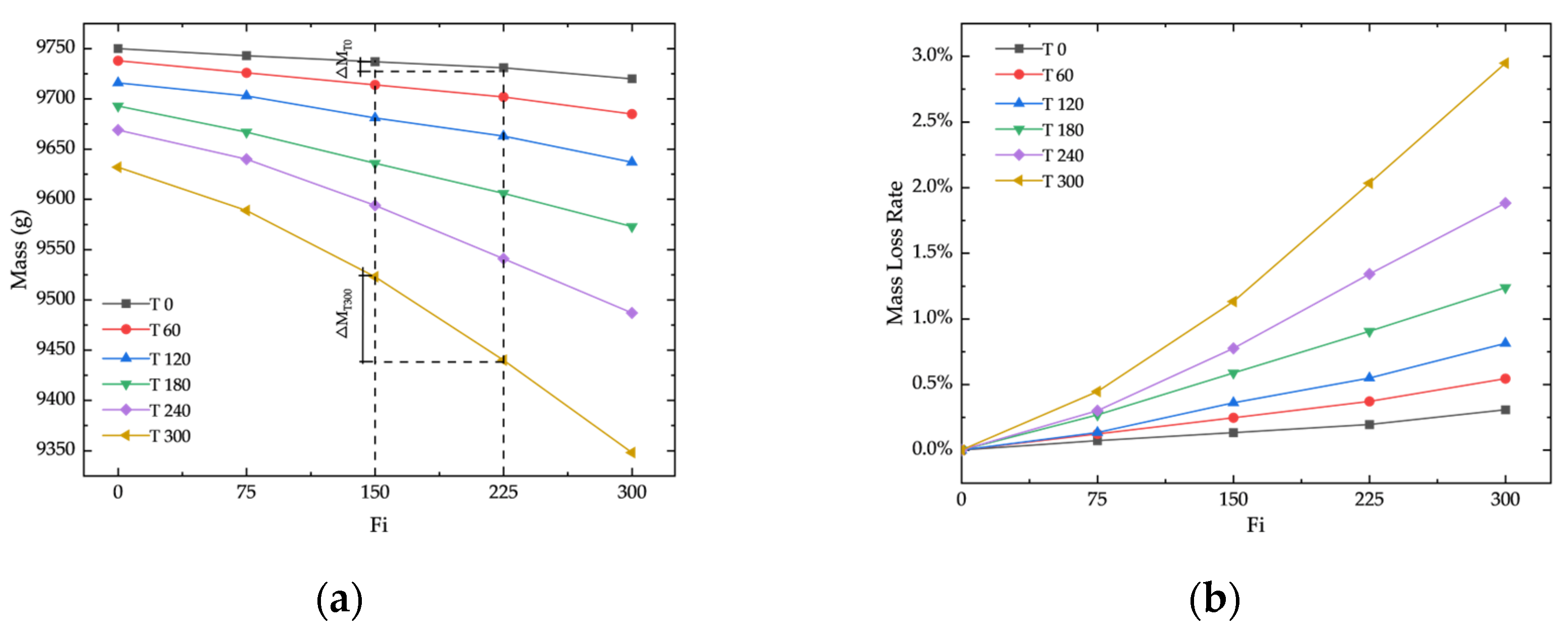
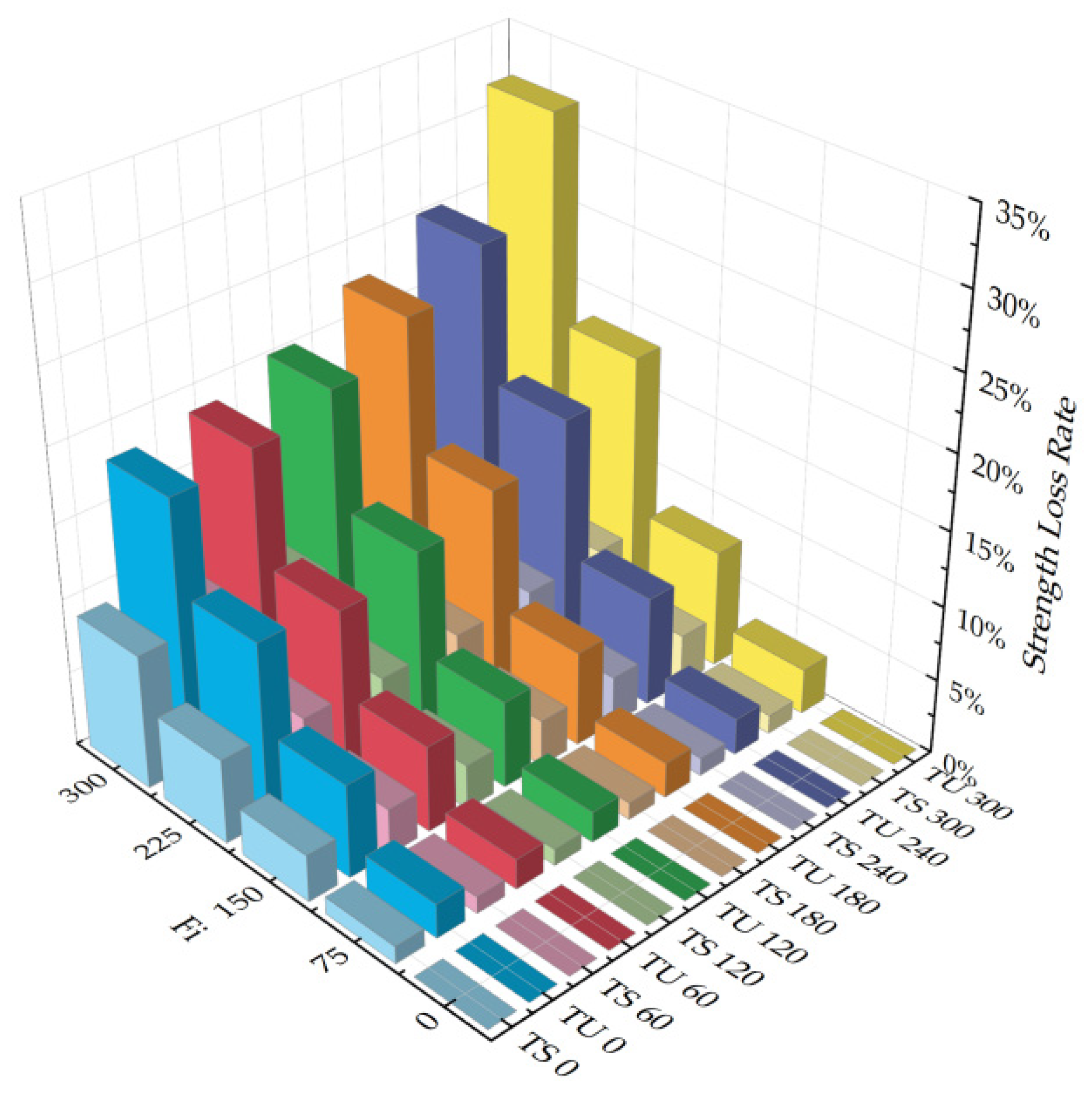
Concrete exhibits significant quality deterioration under combined temperature differential and freeze–thaw cycles. Mass loss increases progressively with both temperature differential and freeze–thaw cycle counts, reaching approximately 3% after 300 temperature differential cycles combined with 300 freeze–thaw cycles. Moreover, the combined cycling effects result in notably greater mass deterioration compared to individual temperature differential or freeze–thaw cycles alone.

(2)

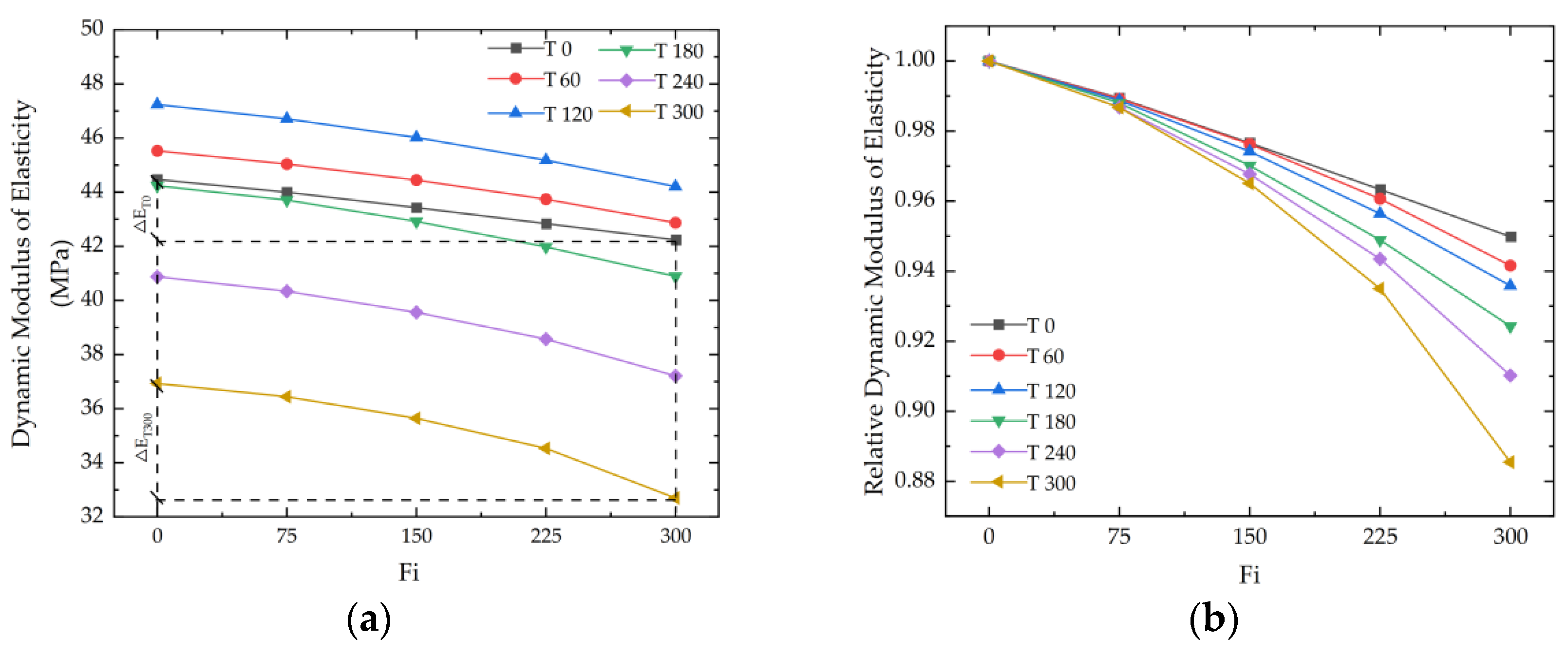
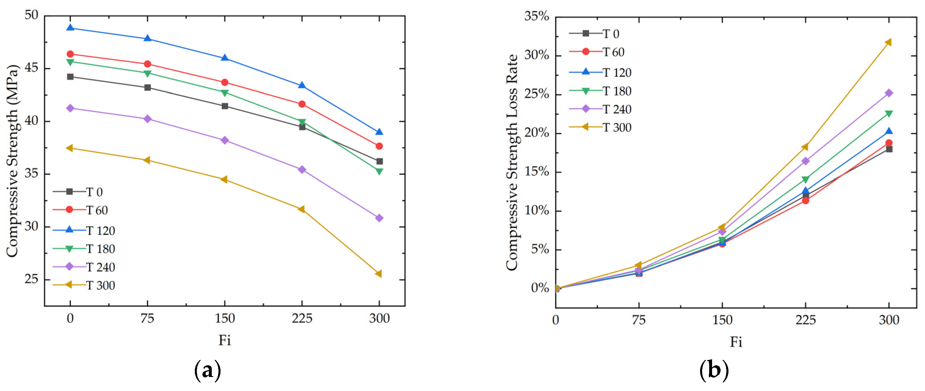
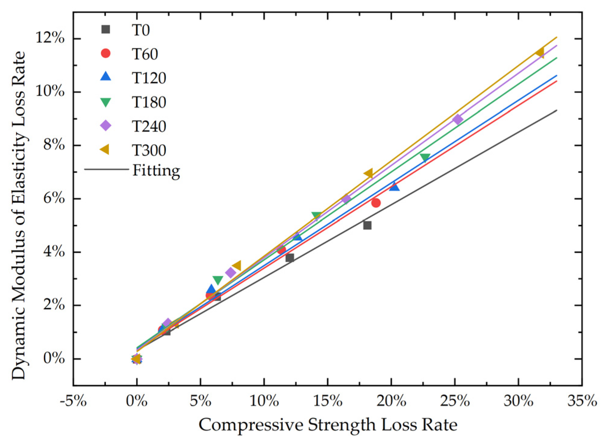
The dynamic modulus and compressive strength of concrete are significantly influenced by temperature differential and freeze–thaw cycling. As the number of temperature fluctuation cycles increases, both the dynamic modulus and strength exhibit a “rise, then fall” trend. Furthermore, an increase in the number of temperature differential cycles leads to a continuous decline in both dynamic modulus and strength. Additionally, under the combined influence of temperature differential and freeze–thaw cycles, a strong linear relationship is observed between compressive strength loss and dynamic modulus loss, indicating that changes in dynamic modulus can quantitatively characterize variations in concrete strength.

(3)

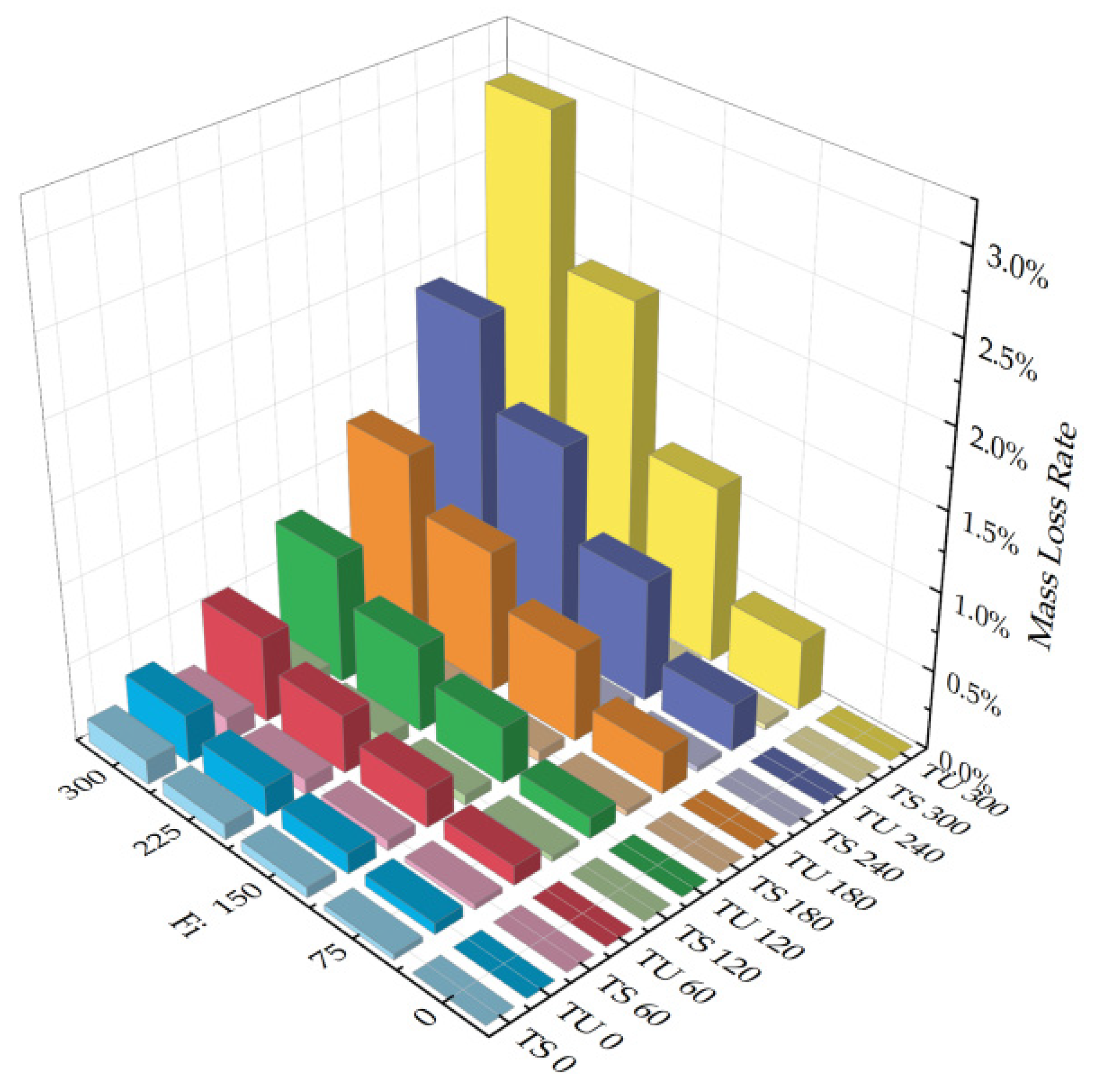
Compared to the superimposed effects of temperature differential cycling and freeze–thaw cycling when acting independently, the combined action of temperature differential and freeze–thaw cycles exhibited significantly greater impacts on the mass, dynamic elastic modulus, and axial compressive strength of cement concrete. Under the condition of 300 temperature differential cycles combined with 300 freeze–thaw cycles, the combined effect was found to be 18 times greater in terms of mass loss rate, 3.7 times greater in terms of dynamic modulus reduction rate, and 1.8 times greater in terms of axial compressive strength loss rate, relative to the sum of the individual effects. These findings indicate that the coupled temperature differential–freeze–thaw action further intensifies the degradation of cement concrete.

(4)

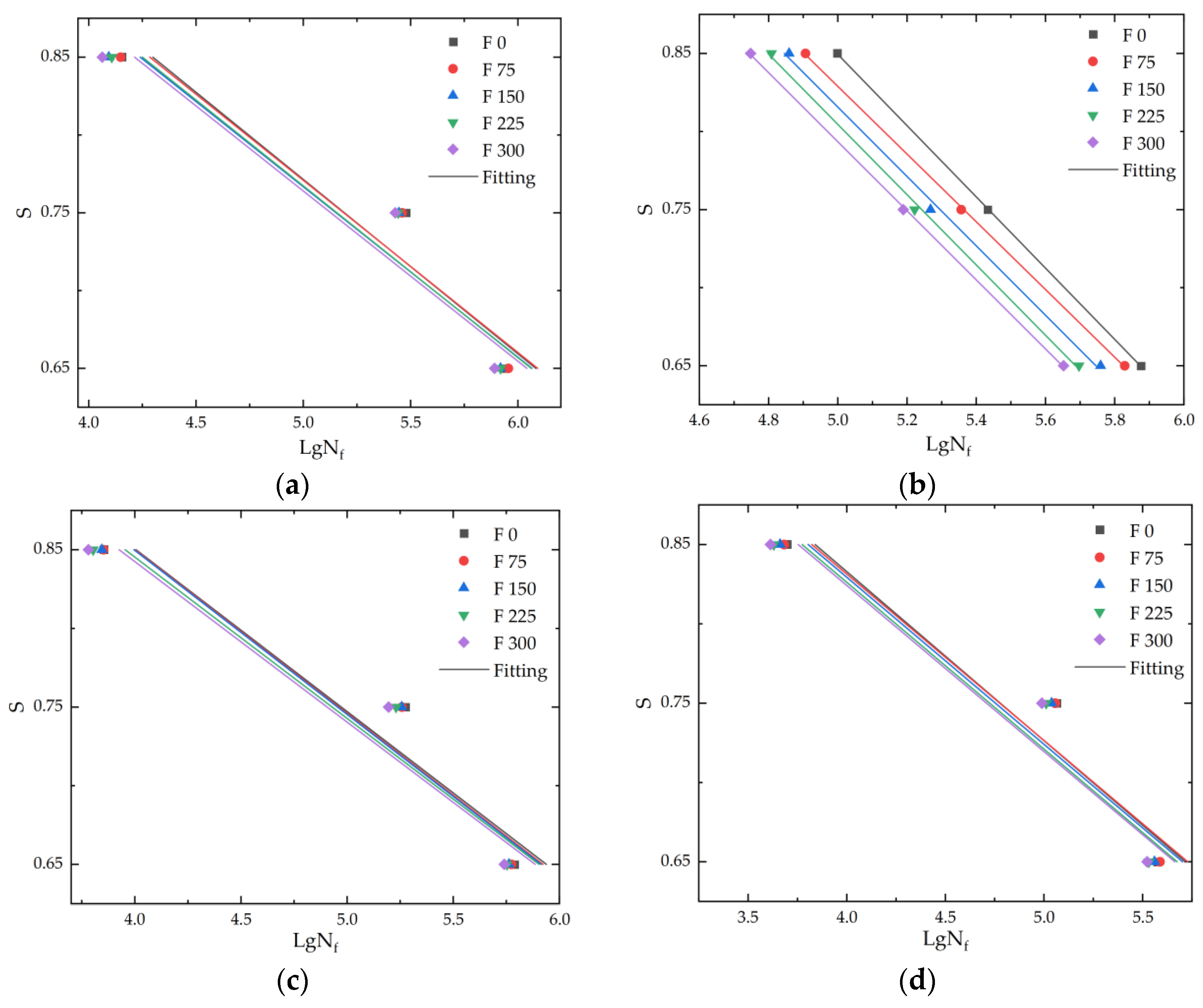
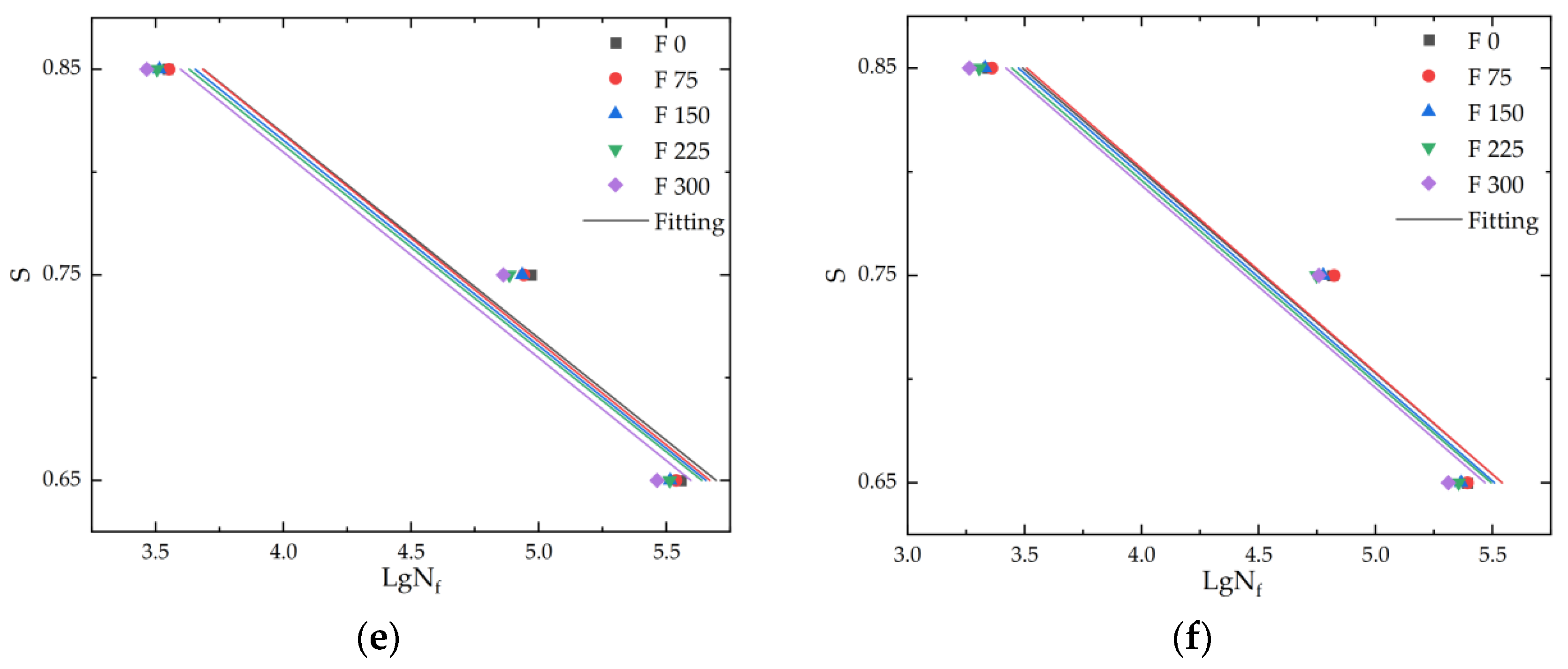
The parameters of the two-parameter Weibull distribution describing cement concrete fatigue life were estimated using the method of moments. Kolmogorov–Smirnov (K-S) tests confirmed a high degree of conformity between the experimental fatigue life data and the two-parameter Weibull distribution, verifying its suitability in accurately characterizing fatigue life under the combined environmental effects of temperature differential and freeze–thaw cycles.

(5)

The S-N_f curves of cement concrete after temperature differential freeze–thaw cycle were fitted using an exponential function. It was found that the reduction in fatigue life after 300 freeze–thaw cycles without temperature differential cycling was 1.22%. However, under the combined influence of temperature differential and freeze–thaw cycling, this reduction can be as high as 4.40%. This demonstrates that the combined effect of temperature differential and freeze–thaw cycling accelerates the deterioration of the durability of cement concrete.

In summary, this study systematically revealed the significant impact of the combined action of temperature differential cycling and freeze–thaw cycling on the performance of cement concrete. Statistical analyses of mass loss, dynamic elastic modulus, axial compressive strength, and fatigue life consistently demonstrated that, under coupled environmental loading, the degradation process of concrete is markedly accelerated, exhibiting a level of damage intensity and rate far beyond the superposition of individual effects. This nonlinear synergistic effect indicates that the material property parameters obtained under conventional test conditions may not fully reflect the complex deterioration mechanisms experienced in real-world service environments. Particularly in terms of fatigue life, although current standards generally adopt 2 million cycles as the design target for the axial compressive fatigue life of cement concrete, extensive engineering practice has shown that many structures experience fatigue failure at much lower cycle counts, thereby posing serious concerns for structural safety and durability. A primary reason lies in the current design frameworks, which often fail to incorporate environmental factors such as temperature differential cycling and freeze–thaw cycling into the fatigue life evaluation systems. Based on the findings of this study, it is suggested that the coupled effects of temperature differential and freeze–thaw cycling should be explicitly considered in the durability design and service life assessment of concrete structures. Such consideration is essential for achieving a more scientific, rational, and environmentally adaptive design approach. Moreover, this work provides both theoretical support and experimental data that can guide future performance-oriented optimization of concrete materials for use in cold and complex climatic regions.

Future studies may consider integrating end-to-end vision models into concrete performance analysis to establish a deeper correlation between microcrack evolution and macroscopic mechanical degradation. In subsequent work, high-resolution cameras or microscopes can be employed to acquire multi-view images of specimen surfaces. These images can then be processed using advanced deep learning frameworks—such as the DeepLab model [40], which leverages Atrous Spatial Pyramid Pooling (ASPP) and depthwise separable convolutions—for the pixel-level semantic segmentation of microcracks, enabling the extraction of morphological indicators such as total crack length, width distribution, connectivity, and crack density. Additionally, lightweight networks based on EfficientNet [41] can utilize compound scaling strategies to efficiently encode the texture features surrounding cracks. When combined with feature alignment and temporal tracking algorithms, these methods can support the quantitative analysis of crack propagation rates and the emergence of new cracks. By integrating these microstructural crack parameters with dynamic modulus, compressive strength, and fatigue life data through multimodal regression or joint predictive modeling, we aim not only to establish a quantitative relationship between crack evolution and mechanical deterioration, but also to significantly enhance the accuracy of concrete life prediction under temperature differential and freeze–thaw cycling conditions.

References

1. Collins, A.R. The destruction of concrete by frost. J. Inst. Civ. Eng. 1944, 23, 29–41. [Google Scholar] [CrossRef]
2. Powers, T.C. A working hypothesis for further studies of frost resistance of concrete. J. Am. Concr. Inst. 1945, 16, 245–272. [Google Scholar]
3. Powers, T.C.; Helmuth, R.A. Theory of volume changes in hardened portland cement paste during freezing. In Proceedings of the Highway Research Board Proceedings, Washington, DC, USA, 13–16 January 1953. [Google Scholar]
4. Litvan, G.G. Frost action in cement paste. Matériaux Constr. 1973, 6, 293–298. [Google Scholar] [CrossRef]
5. Mehta, P.K.; Schiessl, P.; Raupach, M. Performance and Durability of Concrete and Cement Systems. In Proceedings of the 9th International Congress on the Chemistry of Cement, New Delhi, India, 23–28 November 1992; Volume 1, pp. 571–659. [Google Scholar]
6. Setzer, M.J. Micro-ice-lens formation in porous solid. J. Colloid Interface Sci. 2001, 243, 193–201. [Google Scholar] [CrossRef]
7. Penttala, V. Surface and internal deterioration of concrete due to saline and non-saline freeze-thaw loads. Cem. Concr. Res. 2006, 36, 921–928. [Google Scholar] [CrossRef]
8. Shisheng, S. Effect of freezing-thawing cycles on mechanical properties of concrete. China Civ. Eng. J. 1997, 30, 35–42. [Google Scholar]
9. Shang, H.; Song, Y. Experimental study on the performance of ordinary concrete after freeze-thaw cycles. China Concr. Cem. Prod. 2005, 2, 9–11. [Google Scholar]
10. Shang, S. Experimental Study on Strength of Air-Entrained Concrete Under Multiaxial Loads After Freeze-Thaw Cycles. Ph.D. Thesis, Dalian University of Technology, Dalian, China, 2006. [Google Scholar]
11. Cho, T. Prediction of cyclic freeze–thaw damage in concrete structures based on response surface method. Constr. Build. Mater. 2007, 21, 2031–2040. [Google Scholar] [CrossRef]
12. Vesikari, E. Service life design of concrete structures with regard to the frost resistance of concrete. Nord. Concr. Res. 1987, 5, 215–228. [Google Scholar]
13. Gan, Y.; Sun, C.; Liao, W. One service-life prediction model for the concrete based on the reliability and damage theories narration and establishment of the model. J. Chin. Ceram. Soc. 2001, 29, 530–534. [Google Scholar]
14. Gan, Y.; Sun, C.; Liao, W. One service-life prediction model for the concrete based on the reliability and damage theories verification and application of the model. J. Chin. Ceram. Soc. 2001, 29, 535–540. [Google Scholar]
15. Ou, L.; Sun, Z.M. Flexural fatigue-life reliability of frost-damaged concrete. J. Zhejiang Univ. (Eng. Sci.) 2017, 51, 1074–1081, 1103. [Google Scholar]
16. Boyd, A.J.; Leone, A. Effect of freeze-thaw cycling on fatigue behaviour in concrete, Conference Series: Materials Science and Engineering. IOP Publ. 2019, 652, 012028. [Google Scholar]
17. Kuosa, H.; Ferreira, R.; Holt, E.; Leivo, M.; Vesikari, E. Effect of coupled deterioration by freeze-thaw, carbonation and chlorides on concrete service life. Cem. Concr. Compos. 2014, 47, 4732–4740. [Google Scholar] [CrossRef]
18. Al-Tayyib, A.J.; Baluch, M.H.; Sharif, A.F.M.; Mahamud, M.M. The effect of thermal cycling on the durability of concrete made from local materials in the arabian gulf countries. Cem. Concr. Res. 1990, 19, 131–142. [Google Scholar] [CrossRef]
19. Kanellopoulos, A.; Farhat, F.A.; Nicolaides, D.; Karihaloo, B.L. Mechanical and fracture properties of cement-based bi-materials after thermal cycling. Cem. Concr. Res. 2009, 39, 1087–1094. [Google Scholar] [CrossRef]
20. Shokrieh, M.M.; Heidari-Rarani, M.; Shakouri, M.; Kashizadeh, E. Effects of thermal cycles on mechanical properties of an optimized polymer concrete. Constr. Build. Mater. 2011, 25, 3540–3549. [Google Scholar] [CrossRef]
21. Heidari-Rarani, M.; Aliha, M.R.M.; Shokrieh, M.M.; Ayatollahi, M.R. Mechanical durability of an optimized polymer concrete under various thermal cyclic loadings—An experimental study. Constr. Build. Mater. 2014, 64, 308–315. [Google Scholar] [CrossRef]
22. Huang, H.; An, M.; Wang, Y.; Yu, Z.; Ji, W. Effect of environmental thermal fatigue on concrete performance based on meso structural and micro structural analyses. Constr. Build. Mater. 2019, 207, 450–462. [Google Scholar] [CrossRef]
23. Li, Z.; Shang, H.; Xiao, S.; Yang, L.; Li, Z. Effect of thermal fatigue on mechanical properties and micro structure of concrete. Bull. Chin. Ceram. Soc. 2022, 41, 825–832. [Google Scholar]
24. Oh, B.H. Cumulative damage theory of concrete under variable- amplitude fatigue loadings. ACI Mater. J. 1991, 88, 41–48. [Google Scholar]
25. Zhou, X.; Wu, J. Preliminary research on fatigue behavior of concrete after exposed to high temperature. Ind. Constr. 1996, 5, 33–35. [Google Scholar]
26. Zhao, D.; Gao, P.; Jia, H.J. Performance degradation of high strength concrete(hsc) after different-high-temperature history. J. Vib. Shock 2018, 37, 240–248. [Google Scholar]
27. Xue, G.; Zhu, H.; Xu, S.; Dong, W. Fatigue performance and fatigue equation of crumb rubber concrete under freeze–thaw cycles. Int. J. Fatigue 2023, 168, 107456. [Google Scholar] [CrossRef]
28. Zhu, X.; Chen, X.; Pan, F. Reliability analysis of fatigue life of self compacting concrete subjected to freeze thaw damage. J. Harbin Inst. Technol. 2023, 55, 118–127. [Google Scholar]
29. Najam, F.A.; Qureshi, M.I.; Warnitchai, P.; Mehmood, T. Prediction of nonlinear seismic demands of high-rise rocking wall structures using a simplified modal pushover analysis procedure. Struct. Des. Tall Spec. Build. 2018, 27, e1506. [Google Scholar] [CrossRef]
30. Khan, A. Gender-based emergency preparedness and awareness: Empirical evidences from high-school students of Gilgit, Pakistan. Environ. Hazards 2020, 20, 416–431. [Google Scholar] [CrossRef]
31. JGJ 55-2011; Specification for Mix Proportion Design of Ordinary Concrete. Ministry of Housing and Urban-Rural Development of the People’s Republic of China: Beijing, China, 2011.
32. GB/T 50081-2019; Standard for Test Methods of Concrete Physical and Mechanical Propryies. Ministry of Housing and Urban-Rural Development of the People’s Republic of China: Beijing, China, 2019.
33. GB/T 50082-2009; Standard for Test Methods of Long-Term Performance and Durability of Ordinary Concrete. Ministry of Housing and Urban-Rural Development of the People’s Republic of China: Beijing, China, 2009.
34. Tao, C.; Dong, L.; Fan, W.; Yu, T. Experimental Study on the Compressive Strength and Fatigue Life of Cement Concrete under Temperature Differential Cycling. Materials 2023, 16, 7487. [Google Scholar] [CrossRef]
35. Cui, K.; Xu, L.; Li, X.; Hu, X.; Huang, L.; Deng, F.; Chi, Y. Fatigue life analysis of polypropylene fiber reinforced concrete under axial constant- amplitude cyclic compression. J. Clean. Prod. 2021, 319, 128610. [Google Scholar] [CrossRef]
36. Zhou, J.; Zhang, Z.; Li, J. Experimental study on compressive fatigue performance of recycled concrete under temperature cycling. J. Hubei Univ. Technol. 2023, 38, 71–75. [Google Scholar]
37. Jiang, R. Weibull Model Family Properties, Parameter Estimation and Applications; Science Press: Beijing, China, 1999. [Google Scholar]
38. Singh, S.P.; Kaushik, S.K. Flexural fatigue life distributions and failure probability of steel fibrous concrete. Mater. J. 2000, 97, 658–667. [Google Scholar]
39. Kennedy, J.B.; Neville, A.M. Basic Statistical Methods for Engineers and Scientists; International Textbook Company: Scranton, PA, USA, 1964. [Google Scholar]
40. Song, Z.; Zou, S.; Zhou, W.; Huang, Y.; Shao, L.; Yuan, J.; Gou, X.; Jin, W.; Wang, Z.; Chen, X.; et al. Clinically applicable histopathological diagnosis system for gastric cancer detection using deep learning. Nat. Commun. 2020, 11, 4294. [Google Scholar] [CrossRef] [PubMed]
41. Kabir, H.; Wu, J.; Dahal, S.; Joo, T.; Garg, N. Automated estimation of cementitious sorptivity via computer vision. Nat. Commun. 2024, 15, 9935. [Google Scholar] [CrossRef] [PubMed]
Figure 1. Illustration of the temperature differential cycling mechanism [34].
Buildings 15 01566 g001
Figure 2. Changes in mass of specimens under the combined effects of temperature differential and freeze–thaw cycling: (a) changes in mass; (b) mass loss.
Buildings 15 01566 g002
Figure 3. Mass loss rate under the separate and combined effects of temperature differential and freeze–thaw cycling.
Buildings 15 01566 g003
Figure 4. The variation in the dynamic modulus of elasticity of concrete specimens under the combined effects of temperature differential and freeze–thaw cycling: (a) variation in the dynamic modulus of elasticity; (b) normalized dynamic modulus of elasticity.
Buildings 15 01566 g004
Figure 5. Dynamic modulus of elasticity loss rate under the separate effects of temperature differential cycling, freeze–thaw cycling, and the combined effects of the two cycles.
Buildings 15 01566 g005
Figure 6. Variation in strength of concrete specimens under the combined effects of temperature differential and freeze–thaw cycling: (a) variation in strength; (b) strength loss rate.
Buildings 15 01566 g006
Figure 7. Fitting curve for the relationship between the loss of dynamic modulus of elasticity and strength loss.
Buildings 15 01566 g007
Figure 8. Strength loss rate of concrete under the separate and combined effects of temperature differential cycling and freeze–thaw cycling.
Buildings 15 01566 g008
Figure 9. S-Nf curves for concrete under different temperature differential and freeze–thaw cycles: (a) T = 0; (b) T = 60; (c) T = 120; (d) T = 180; (e) T = 240; (f) T = 300.
Buildings 15 01566 g009aBuildings 15 01566 g009b