Dynamic Modeling, Trajectory Optimization, and Linear Control of Cable-Driven Parallel Robots for Automated Panelized Building Retrofits ^†

Abstract

The construction industry faces a growing need for automation to reduce costs, improve accuracy and productivity, and address labor shortages. One area that stands to benefit significantly from automation is panelized prefabricated building envelope retrofits, which can improve a building’s energy efficiency in heating and cooling interior spaces. In this paper, we propose using cable-driven parallel robots (CDPRs), which can effectively lift and handle large objects, to install these panels. However, implementing CDPRs presents significant challenges because of their nonlinear dynamics, complex trajectory planning, and precise control requirements. To tackle these challenges, this work focuses on a new application of established control and trajectory optimization theories in a CDPR simulation of a building envelope retrofit under real-world conditions. We first model the dynamics of CDPRs, highlighting the critical role of damping in system behavior. Building on this dynamic model, we formulate a trajectory optimization problem to generate feasible and efficient motion plans for the robot under operational and environmental constraints. Given the high precision required in the construction industry, accurately tracking the optimized trajectory is essential. However, challenges such as partial observability and external vibrations complicate this task. To address these issues, a Linear Quadratic Gaussian control framework is applied, enabling the robot to track the optimized trajectories with precision. Simulation results show that the proposed controller enables precise end effector positioning with errors under 4 mm, even in the presence of external wind disturbances. Through comprehensive simulations, our approach allows for an in-depth exploration of the system’s nonlinear dynamics, trajectory optimization, and control strategies under controlled yet highly realistic conditions. The results demonstrate the feasibility of CDPRs for automating panel installation and provide insights into their practical deployment.

1. Introduction

The use of robotics and automation in construction has the potential to alleviate labor shortages, increase worker safety, and reduce construction time and overall costs. One promising application is automating building envelope retrofits using overclad prefabricated panels. Building envelope retrofits significantly enhance building energy performance and sustainability by installing thermal insulation panels on existing exterior walls [1]. Traditional methods for installing overclad prefabricated panels on multistory buildings often depend on manual labor or crane assistance. However, these approaches are susceptible to installation errors, pose safety hazards for workers, and are inefficient and logistically challenging, especially in densely populated urban areas with limited space [2]. Cable-driven parallel robots (CDPRs) are parallel mechanisms that use multiple cables to manipulate an end effector [3]. Features such as compact design, reconfigurability, scalability, and a high payload-to-weight ratio make CDPRs suitable for automating overclad prefabricated panel installation. CDPRs can operate in environments where traditional machinery might be impractical, offering enhanced flexibility and precision. In this paper, we propose CDPRs as a promising solution for the manipulation of prefabricated panels in building envelope retrofits (see Figure 1).

Despite its potential, the implementation of CDPRs in building envelope retrofitting applications introduces several technical challenges. The dynamics of CDPRs are inherently nonlinear. Modeling and analyzing these dynamics are essential for predicting system behavior and ensuring stable operation. Another significant challenge in panelized building retrofits is generating trajectories for the robot to track. The trajectory planning process must guarantee that the robot can safely maneuver the panels from the pickup location to the desired pose on the facade while adhering to hard and soft constraints and optimizing performance metrics such as energy consumption or time. Minimizing energy consumption is particularly critical because lifting heavy panels requires substantial force, which can strain the actuation system and potentially exceed its load capacity. Given that these panels can weigh several hundred kilograms, our primary goal is to develop strategies for efficient and smooth load handling. Improved load management not only enhances operational safety and reliability but also reduces costs and extends the lifespan of the equipment. Once the optimal trajectory is generated, an effective controller is essential. Our industry partners have specified that installed panels must maintain an error margin (tolerance) of less than 4 mm to minimize on-site installation errors and rework; otherwise, any gaps outside tolerance could result in air leaks and reduce the energy efficiency of the new envelope. Moreover, the CDPR dynamic system often operates under partial observability, in which not all states can be directly measured, and some states may be observed at varying frequencies because of sensor limitations or noise. External disturbances further affect the robot’s precision. All these real-world challenges demand carefully designed control strategies and optimally selected sensors to estimate states in order to compensate for partial observability and uncertainties, as well as to ensure high performance.

This paper aims to address the above trajectory generation and control-related challenges in construction settings simulated under realistic conditions to show that CDPRs are viable for automating the handling of large prefabricated panels. Our work makes the following primary contributions:

• Dynamic modeling of six–degrees of freedom (6DOF) CDPRs: We model the dynamics of the CDPR used for installing prefabricated panels. Our analysis highlights the critical role of damping in system behavior, an aspect often overlooked in prior studies.
• Trajectory optimization for efficient handling of heavy loads: We formulate a trajectory optimization problem using nonlinear programming techniques to directly minimize objectives of interest, such as minimum effort. Notably, our framework can generate optimal open-loop trajectories over extended durations (e.g., 20 s) for a 6DOF CDPR, a capability that has not been widely demonstrated in prior studies to the best of our knowledge.
• Feedback control strategies for high-precision trajectory tracking: We apply the well-established Linear Quadratic Gaussian (LQG) control framework to estimate the full states and track the optimal trajectory. Although the LQG framework provides a foundation for control, achieving the high-precision requirements of the panel installation process in the construction industry remains challenging. To address this, we evaluate different sensors for state estimation and examine their effectiveness in mitigating external disturbances. Our study offers insights into designing feedback control strategies that integrate optimal control with state estimation, ensuring accurate trajectory tracking despite uncertainties and environmental factors.

Our methodology applies well-established trajectory optimization and feedback control theories for CDPRs in panelized building retrofits via simulations that mimic the conditions of real-world retrofit scenarios. The results demonstrate the viability of CDPRs for precisely handling prefabricated panels. By addressing the challenges of nonlinear dynamics, trajectory optimization, and control under uncertainty through extensive simulations, we open a pathway toward the practical adoption of CDPR technology in real-world panelized building envelope retrofits.

The remainder of this paper is organized as follows: Section 2 reviews related work on CDPRs in construction and existing approaches to trajectory planning and control. Section 3 models dynamics for 6DOF CDPRs. Section 4 presents the formulation of the trajectory optimization problem using nonlinear programming and addresses the solution methods. Section 5 introduces the LQG control framework and explains its implementation under partial observability and varying observation frequencies. Section 6 provides simulation results and analyzes the performance of the proposed methods under various scenarios. Finally, Section 7 summarizes the paper and describes the future development plan of a real-world CDPR system.

2. Related Work

2.1. CDPRs in Robotic Construction

Recently, CDPRs have received attention across various fields and applications because of their desirable characteristics, such as scalability, reconfigurability, compact design, and high payload-to-weight ratio. They have been widely investigated in construction applications such as bricklaying [4,5], 3D printing [6,7], and solar power plant assembly [8]. Murphy et al. developed a planar CDPR for cooperative modular manipulation, enabling CDPRs to assist in construction tasks and gap-crossing scenarios [9]. For building envelope applications, Izard et al. explored the use of eight-cable CDPRs for inspecting building facades [10]. In addition, Iturralde et al. designed and implemented an eight-cable CDPR model for modular curtain wall installation in real-world applications [11]. Their work examined whether CDPRs could achieve sufficient accuracy for installing curtain wall modules and reduce manual installation time. The experiments were conducted in two near-realistic demonstration buildings and revealed an absolute installation accuracy of the curtain wall module system ranging from 4 to 23 mm. The study also analyzed the time required for setting up the CDPR, as well as for installing the brackets and curtain walls. The time analysis indicated that the CDPR setup was the most time-consuming step.

In panelized building retrofits, current construction practices typically rely on manual labor assisted by cranes, with the positioning of prefabricated panels verified only after placement. This reactive approach can lead to significant delays if misalignment occurs, as corrections typically require one to two hours of additional work, including filling gaps, modifying panels, or reinstalling them entirely. In contrast, the CDPR system proposed in this study allows for real-time correction of positioning errors during installation, offering a proactive alternative. This is achieved through the design of an effective feedback controller and the strategic selection of sensors within the feedback loop. By allowing for precise adjustments during the installation process, the system enhances placement accuracy while minimizing the need for costly and time-intensive post-installation corrections, highlighting a significant advantage of CDPR-based automation in prefabricated panel installation settings. Our previous work investigated the wrench-feasible workspace for various cable configurations, focusing primarily on four-cable planar models and eight-cable 3D models [2]. This paper extends that research by exploring essential trajectory optimization and control strategies within the wrench-feasible workspace, which are crucial for the successful implementation of CDPRs in automated panelized building retrofits.

2.2. CDPR Trajectory Planning

A substantial body of literature on trajectory generation and optimization for CDPRs exists. Nevertheless, many of the methods in the literature exhibit limitations that restrict their applicability to complex tasks. Some approaches consider only translational movements without accounting for rotational dynamics, and others generate trajectories for short durations—typically less than 2 s—as seen in works by Badrikouhi and Bamdad [12] and Bamdad [13]. Additionally, several methods neglect the dynamic aspects of the system [14,15], which can lead to suboptimal performance in practical applications.

In one of the earliest works on CDPR trajectory planning [16], Behzadipour and Khajepour proposed a methodology for generating time-optimal trajectories. However, this approach does not guarantee the continuity of cable tensions and is restricted to purely translational motions. Bamdad and Khajepour [13] later used Pontryagin’s maximum principle for trajectory and time optimization but focused on a very short time frame of less than 2 s, limiting their method’s applicability to longer tasks.

Polynomial-based trajectory generation is a common technique employed in CDPR planning because of its computational efficiency and ability to produce smooth motions [17]. Although this method is effective for simple and short-duration trajectories, it may not yield the optimal solutions for complex trajectories or longer motions in which the system dynamics play a significant role.

In one study [15], the trajectory planning of mobile CDPRs is addressed using the direct transcription method. The authors’ approach involves the optimization of positions and velocities for both the mobile bases and the moving platform. However, this work does not consider the dynamics of the CDPR and optimizes only over 11 discrete points, which are subsequently connected using cubic splines. The system studied comprises four cables and does not incorporate rotational dynamics. Similarly, a paper by Hasan et al. [14] presents an optimized path-planning approach for CDPRs using the traveling salesman problem, a branch-and-bound algorithm for a pick-and-place task. Their trajectory consists of three point-to-point linear motions connected by two arc segments designed for a four-cable CDPR without considering rotational movements or system dynamics. The study assumes a constant-speed CDPR, which may oversimplify real-world scenarios.

A paper by Korayem et al. [18] presents an optimal motion planning approach for nonlinear dynamic systems, specifically applied to a spatial six-cable robot, using the state-dependent Riccati equation method. The method produced relatively long optimal trajectories, with some simulations taking around 12 s. However, rotational motion was not explicitly considered in the experiments. Additionally, the method relies on careful tuning of gain matrices, which can be problem-dependent. Furthermore, the sudden changes in motor torques during obstacle avoidance experiments suggest that the approach lacks inherent smoothness, which could lead to instabilities in real-world implementations.

These limitations underscore the need for more comprehensive trajectory generation methods that can handle both translational and rotational dynamics over longer durations while ensuring continuous and smooth cable tension and accounting for the full system dynamics. Nonlinear programming techniques can address these challenges by directly incorporating system dynamics and constraints into the optimization problem, enabling the generation of optimal trajectories for complex, long-duration tasks. Section 4 details our approach to addressing these challenges using nonlinear programming.

2.3. CDPR Controllers

Many studies have explored state estimation and control strategies for CDPRs, including sliding mode control [19], model predictive control [20], proportional–integral–derivative (PID)–based control [21], and extended Kalman filter–based state estimation [22], among others. Le et al. [22] proposed an approach using an extended Kalman filter to integrate inertial measurement unit (IMU) data, including accelerometer and rate gyroscope readings, with forward kinematics for estimating the pose of a CDPR. Simulations on a 6DOF CDPR with eight cables demonstrated position estimation accuracy at the centimeter level and rotation errors within a few degrees. These results indicate that IMU data alone may be insufficient to meet the millimeter-level accuracy demands of the construction industry. A PD controller was employed in a spatial object tracking CDPR [21], and feedback from a gyro sensor, IMUs, and encoders was used to compute position errors. However, in general, PID controllers, because of their reliance on static gains, exhibit sensitivity to operating conditions, leading to inconsistent performance across the workspace and a lack of predictive capability near control limits [23]. To address such limitations, Santos et al. [20] developed a model predictive control strategy for 6DOF CDPRs, explicitly incorporating cable tension limits into the control framework. Chen [24] proposed a locally optimal tracking controller for CDPR control based on a time-varying LQG controller. The tracking performance was validated on a four-cable planar CDPR. However, the studies of Santos et al. and Chen both lack study and experimental validation under conditions of partial observability or external disturbances.

In panelized building envelope retrofits, minimizing installation errors is critical because even small inaccuracies can lead to costly rework or if overlooked, can compromise airtightness. Achieving high precision requires addressing challenges such as partial observability and external disturbances. LQG control offers a balance between control performance and robustness while being computationally efficient—an essential feature for real-time control in CDPRs, which are large systems requiring high-frequency control. Given the well-established effectiveness of the LQG control strategy, our focus is on leveraging the strategy for state estimation and disturbance rejection to meet the precision requirements of the construction industry. In robotics, various sensors—such as IMUs, cameras, and motion capture systems—can be used for state estimation. Additionally, laser trackers, which are widely used in construction for their high precision, can also be used for state estimation. We aim to explore and evaluate these options to enhance state estimation and panel installation precision. Section 5 discusses the application of the LQG framework for state estimation and control, examines different sensor combinations for state observation, and provides guidance on selecting sensors to improve accuracy in CDPR-based construction applications.

3. CDPR Dynamic Modeling and Analysis

In this section, we model the dynamics of the CDPR and then analyze the dynamic behavior of two different CDPR configurations using Jacobian linearization. Finally, we highlight the importance of incorporating damping in dynamic modeling.

3.1. Dynamic Model

The conceptual model of a CDPR is illustrated in Figure 2. The fixed frame (blue) $\mathit{F}={\left[\begin{array}{ccc}{F}_x& F_y& F_z\end{array}\right]}^T$ sets the dimensions of the CDPR in the world coordinate system $\mathcal{A}$. The CDPR manipulates the end effector (red) $\mathit{P}={\left[\begin{array}{ccc}{P}_{x^{\prime }}& P_{y^{\prime }}& P_{z^{\prime }}\end{array}\right]}^T$, which defines the dimensions of the panel in the rotating coordinate system $\mathcal{B}$. Note that in real-world panel installation using CDPRs, the end effector serves as the panel carrier and may be bigger than the panel itself. Finally, n cables connect the panel to the frame. In CDPRs, the cable end connected to the frame runs through pulleys and cable drums to facilitate the winding and unwinding of the cable. However, in this study, we do not model the geometry or dynamics of the winding mechanism. Consider the following vectors for $i\in \{1,\dots ,n\}$, according to Figure 2:

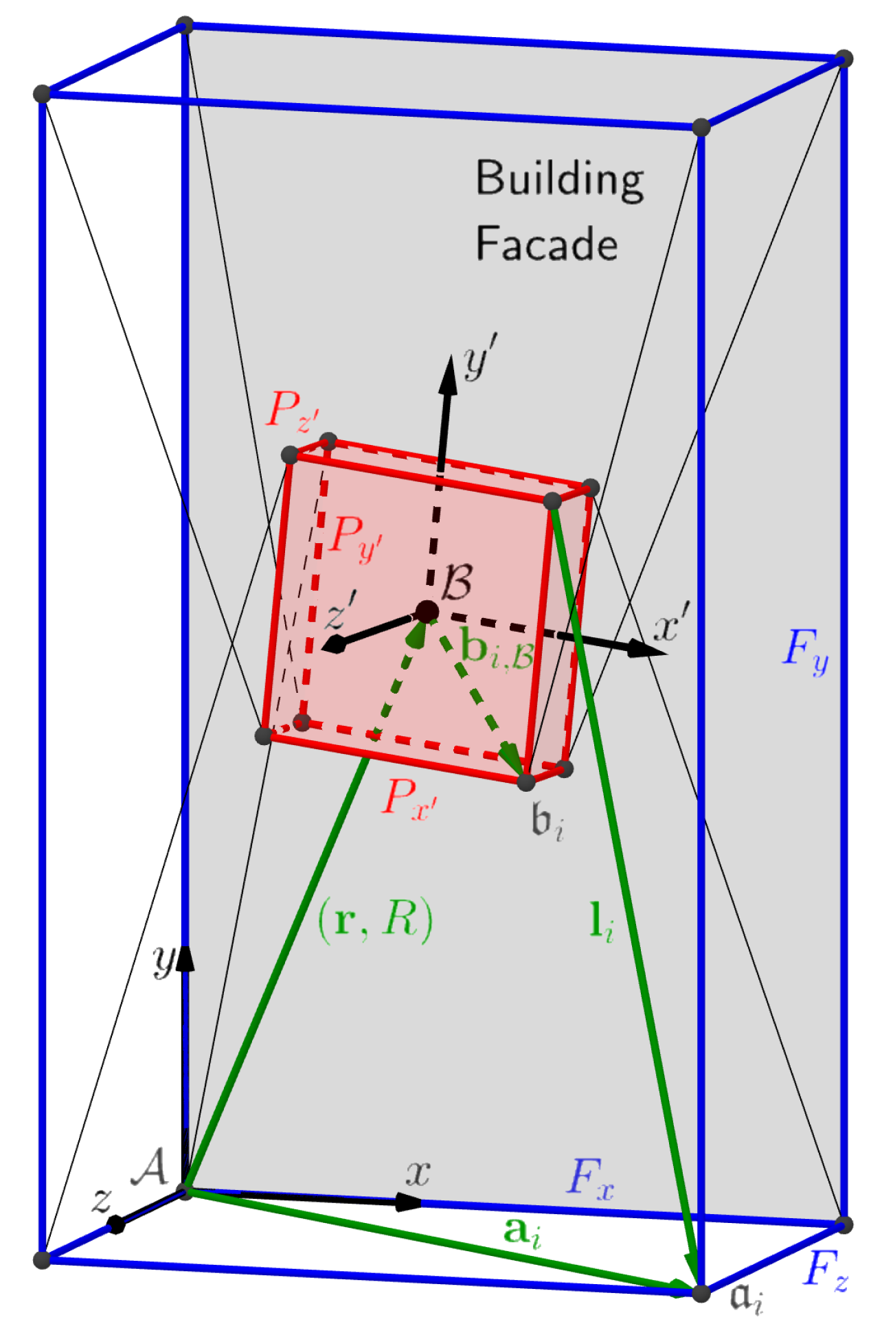
• The constant vectors ${\mathbf{a}}_i$ denote the proximal anchor points ${\mathfrak{a}}_i$ in the frame with respect to $\mathcal{A}$.
• The constant vectors ${\mathbf{b}}_{i,\mathcal{B}}$ denote the distal anchor points ${\mathfrak{b}}_i$ in the panel with respect to $\mathcal{B}$.
• The pose $(\mathit{r},R)$ is defined by the location of the panel’s center of mass $\mathit{r}={\left[\begin{array}{ccc}{r}_x& r_y& r_z\end{array}\right]}^T$ relative to $\mathcal{A}$ and the orientation of the panel’s frame of reference $\mathcal{B}$ relative to $\mathcal{A}$, denoted by the rotation matrix $R\in S{O}_3$.
• The cable vectors ${\mathit{l}}_i={\mathbf{a}}_i-(\mathit{r}+R{\mathbf{b}}_{i,\mathcal{B}})$ are functions of the panel pose calculated relative to $\mathcal{A}$.
• The cable forces ${\mathit{f}}_i=f_i{\mathit{l}}_i/\parallel {\mathit{l}}_i\parallel$ have $f_i\ge 0$ tension acting on the cables ($\parallel ·\parallel$ denotes the Euclidean norm).

The translational motion of the panel is defined in terms of the acceleration of its center of mass, which is measured from the inertial frame of reference $\mathcal{A}$. Therefore, the Newton equations of translational motion, neglecting frictional forces, can be written as follows [25]:

$$\begin{array}{cc}\hfill {\displaystyle \frac{d}{dt}}\mathit{r}& =\mathit{v},\hfill \end{array}$$

(1)

$$\begin{array}{cc}\hfill {\displaystyle \frac{d}{dt}}\mathit{v}& =\mathit{g}+{\displaystyle \frac{1}{m}}\sum _{i=1}^n{f}_i{\displaystyle \frac{{\mathit{l}}_i}{\parallel {\mathit{l}}_i\parallel }}.\hfill \end{array}$$

(2)

Here, $\mathit{v}$ is the velocity of the panel’s center of mass, $\mathit{g}$ is the acceleration due to gravity, and m is the panel’s mass. Because the coordinate system $\mathcal{B}$ is fixed in and moves with the body, the Euler equations of motion written with respect to the coordinate system $\mathcal{B}$ are as follows [25]:

$${\displaystyle \frac{d}{dt}}{\mathit{\omega }}_{\mathcal{B}}=-I_{\mathcal{B}}^{-1}\left({\mathit{\omega }}_{\mathcal{B}}\times I_{\mathcal{B}}{\mathit{\omega }}_{\mathcal{B}}\right)+I_{\mathcal{B}}^{-1}\sum _{i=1}^n{f}_i\left({\mathbf{b}}_{i,\mathcal{B}}\times {\displaystyle \frac{R^T{\mathit{l}}_i}{\parallel {\mathit{l}}_i\parallel }}\right).$$

(3)

Here, $I_{\mathcal{B}}$ is the panel’s inertia tensor (calculated for a solid rectangular cuboid using the panel’s dimensions), and ${\mathit{\omega }}_{\mathcal{B}}$ is its angular velocity observed from the rotating reference frame $\mathcal{B}$ (and × denotes the vector product).

The rate of change in the panel’s orientation can be expressed using three distinct but equivalent formulations:

$$\begin{array}{cccc}\hfill & \mathrm{Rotation}\mathrm{matrix}:\hfill & \hfill {\displaystyle \frac{d}{dt}}R& =R{\left[{\mathit{\omega }}_{\mathcal{B}}\right]}_{\times },\hfill \end{array}$$

(4)

$$\begin{array}{cccc}\hfill & \mathrm{Attitude}\mathrm{quaternion}:\hfill & \hfill {\displaystyle \frac{d}{dt}}\mathsf{q}& ={\displaystyle \frac{1}{2}}\mathsf{q}{\tilde{\mathit{\omega }}}_{\mathcal{B}},\hfill \end{array}$$

(5)

$$\begin{array}{cccc}\hfill & \mathrm{Euler}\mathrm{angles}:\hfill & \hfill {\displaystyle \frac{d}{dt}}\mathbf{\Phi }& =T{\mathit{\omega }}_{\mathcal{B}}.\hfill \end{array}$$

(6)

Here, ${[·]}_{\times }$ denotes the skew-symmetric operator, $\mathsf{q}$ is the unit quaternion linked to the panel orientation, ${\tilde{\mathit{\omega }}}_{\mathcal{B}}$ is the pure quaternion angular velocity, and $\mathbf{\Phi }={\left[\begin{array}{ccc}\phi & \theta & \psi \end{array}\right]}^T$ denotes the Euler angles. The rotation matrix formulation is the most straightforward. However, Equation (4) requires nine states for R in addition to the nine states needed to simulate Equations (1)–(3), resulting in a system with 18 states. The attitude quaternion formulation can reduce the state space to 13 dimensions. However, substituting R with $\mathsf{q}$ implies switching from a matrix vector product to a conjugation operation, which is cumbersome to linearize. Finally, the Euler angles formulation provides the minimum realization of the system with 12 states. However, R has to be decomposed into three elemental rotations, each parameterized by a single Euler angle. In our CDPR applications, these Euler angles are bounded to avoid singularity and ensure wrench feasibility. Consider the following composition order for the elemental rotations: $R=R_z\left(\psi \right)R_y\left(\theta \right)R_x\left(\phi \right)$. Then, the transformation matrix in Equation (6) becomes [26]

$$T=\left[\begin{array}{ccc}1& sin\phi tan\theta & cos\phi tan\theta \\ 0& cos\phi & -sin\phi \\ 0& sin\phi sec\theta & cos\phi sec\theta \end{array}\right].$$

(7)

Equations (1)–(3) and (6) define the minimum system realization of the CDPR when only gravitational and cable forces are considered. Let $x={\left[\begin{array}{cccc}{\mathit{r}}^T& {\mathbf{\Phi }}^T& {\mathit{v}}^T& {\mathit{\omega }}_{\mathcal{B}}^T\end{array}\right]}^T$ be the combined state and $u={\left[\begin{array}{ccc}{f}_1& \cdots & f_n\end{array}\right]}^T$ be the control input. Then, the nonlinear model becomes ${\displaystyle \frac{d}{dt}}x=g(x,u)$.

3.2. Jacobian Linearization

Let ($\overline{x}$, $\overline{u}$) be an equilibrium point, and let ($\delta x=x-\overline{x}$, $\delta u=u-\overline{u}$) be small deviations around the equilibrium. Then, the Jacobian linearization can be written as follows:

$${\displaystyle \frac{d}{dt}}\delta x=A\delta x+B\delta u.$$

(8)

Matrix A can be calculated as

$$A=\left[\begin{array}{cccc}0& 0& {\mathbb{E}}_3& 0\\ 0& T_{\mathbf{\Phi }}\otimes {\mathit{\omega }}_{\mathcal{B}}& 0& T\\ {\displaystyle {\displaystyle \frac{1}{m}}\sum _{i=1}^n{\displaystyle \frac{f_i}{{\parallel {\mathit{l}}_i\parallel }^3}}\Delta L_i}& {\displaystyle {\displaystyle \frac{1}{m}}\sum _{i=1}^n{\displaystyle \frac{f_i}{{\parallel {\mathit{l}}_i\parallel }^3}}\Delta L_i(R_{\mathbf{\Phi }}\otimes {\mathbf{b}}_{i,\mathcal{B}})}& 0& 0\\ {\displaystyle I_{\mathcal{B}}^{-1}\sum _{i=1}^n{\displaystyle \frac{f_i}{{\parallel {\mathit{l}}_i\parallel }^3}}{\left[{\mathbf{b}}_{i,\mathcal{B}}\right]}_{\times }{R}^T\Delta L_i}& {\displaystyle I_{\mathcal{B}}^{-1}\sum _{i=1}^n{\displaystyle \frac{f_i}{{\parallel {\mathit{l}}_i\parallel }^3}}{\left[{\mathbf{b}}_{i,\mathcal{B}}\right]}_{\times }\left[R^T\Delta L_i(R_{\mathbf{\Phi }}\otimes {\mathbf{b}}_{i,\mathcal{B}})+{\parallel {\mathit{l}}_i\parallel }^2(R_{\mathbf{\Phi }}^T\otimes {\mathit{l}}_i)\right]}& 0& -I_{\mathcal{B}}^{-1}\Delta {\Omega }_{\mathcal{B}}\end{array}\right].$$

(9)

Here, ${\mathbb{E}}_s$ denotes the $s\times s$ identity matrix. Other matrix identities are defined below:

$$\begin{array}{cc}\hfill M_{\mathbf{\Phi }}\otimes \mathit{p}& =\left[\begin{array}{ccc}{\displaystyle \frac{\partial M}{\partial \phi }}\mathit{p}& {\displaystyle \frac{\partial M}{\partial \theta }}\mathit{p}& {\displaystyle \frac{\partial M}{\partial \psi }}\mathit{p}\end{array}\right],\hfill \end{array}$$

(10)

$$\begin{array}{cc}\hfill \Delta L_i& ={\mathit{l}}_i{\mathit{l}}_i^T-{\mathit{l}}_i^T{\mathit{l}}_i{\mathbb{E}}_3,\hfill \end{array}$$

(11)

$$\begin{array}{cc}\hfill \Delta {\Omega }_{\mathcal{B}}& ={\left[{\mathit{\omega }}_{\mathcal{B}}\right]}_{\times }{I}_{\mathcal{B}}-{\left[I_{\mathcal{B}}{\mathit{\omega }}_{\mathcal{B}}\right]}_{\times },\hfill \end{array}$$

(12)

where M denotes any 3 × 3 matrix and $\mathit{p}$ denotes any 3D vector. Similarly, matrix B can be calculated as

$$B=\left[\begin{array}{ccc}0& \cdots & 0\\ 0& \cdots & 0\\ {\displaystyle \frac{1}{m}}·{\displaystyle \frac{{\mathit{l}}_1}{\parallel {\mathit{l}}_1\parallel }}& \cdots & {\displaystyle \frac{1}{m}}·{\displaystyle \frac{{\mathit{l}}_1}{\parallel {\mathit{l}}_n\parallel }}\\ I_{\mathcal{B}}^{-1}\left({\mathbf{b}}_{1,\mathcal{B}}\times {\displaystyle \frac{R^T{\mathit{l}}_1}{\parallel {\mathit{l}}_1\parallel }}\right)& \cdots & I_{\mathcal{B}}^{-1}\left({\mathbf{b}}_{n,\mathcal{B}}\times {\displaystyle \frac{R^T{\mathit{l}}_n}{\parallel {\mathit{l}}_n\parallel }}\right)\end{array}\right].$$

(13)

The linearized system was used to understand the dynamic properties of different equilibria and to design a feedback controller for the CDPR to maintain the panel along a predetermined trajectory, even under disturbances.

3.3. CDPR Configurations, Poles, and Damping

To study the use of CDPRs for building envelope retrofits, we used a one-third scaled model of a three-story residential building. The specifications were as follows: the frame’s width, height, and depth were 1.829, 3.124, and 1.219 m, respectively; the panel had dimensions of 0.762, 0.762, and 0.254 m and a mass of 13.6 kg; and the cable forces were constrained between 66 and 1200 N. The CDPRs have eight cables, eight distal anchors, and eight proximal anchors. This paper focuses on investigating the dynamic behavior of the two models shown in Figure 3. They were selected because model 1 is widely used and studied, and model 2 leads to good facade coverage according to our previous work [2].

To understand the dynamic behavior of these two models, we first plotted the poles of the linearized system, corresponding to the eigenvalues of matrix A in Equation (8). Figure 3 shows that the poles of model 1 reside on the imaginary axis. In model 2, however, one of the poles has a positive real part. Therefore, model 1 can develop harmonic oscillator behavior, whereas model 2’s output is likely to increase without bounds, causing the system to be unstable. To evaluate the dynamic responses of these two models, we used the inverse dynamics together with the p-norm method [3] (pp. 80–81) to compute the force trajectories that guide the panel from one pose to another. Given the initial state and generated force trajectory, a SciPy nonlinear system solver was used to simulate the evolution of both models, depicted in Figure 4. Note that model 1 can closely track the planned trajectory with small errors and oscillations in angular velocity. Conversely, model 2 clearly exhibits oscillations and instability. Further analysis indicated that this instability exists in many CDPR models. In real-world systems, friction between moving components plays a significant role in damping out oscillations. Therefore, to match real-world observations of model 2, we need to introduce damping into the system dynamics. Consider adding linear viscous friction in the Newton–Euler equations proportional to the linear and angular velocities as follows:

$${\displaystyle \frac{d}{dt}}x=g(x,u)-Dx,$$

(14)

where $D=\mathrm{diag}\left(\begin{array}{cccc}0,& 0,& {\displaystyle \frac{{\mu }_{\mathit{v}}}{m}}{\mathbb{E}}_3,& I_{\mathcal{B}}^{-1}{\mu }_{\mathit{\omega }}\end{array}\right)$ is block diagonal. Then, the nonlinear model can be written as ${\displaystyle \frac{d}{dt}}x=h(x,u)$. Figure 5 shows how the same initial pose and force trajectory affect the damped system dynamics of model 2.

Figure 4 and Figure 5 demonstrate that damping plays a crucial role in the dynamic modeling of CDPRs; however, we observe a discrepancy in previous studies: not all have explicitly integrated damping, potentially causing confusion. Papers that explicitly model damping include papers by Mamidi and Bandyopadhyay [27] and Miermeister and Pott [28]. However, several other papers, such as those by Zi et al. [29], Lamaury and Gouttefarde [30], Sheng et al. [31], and Wu et al. [4], do not explicitly incorporate damping into their dynamic modeling. From our simulation results, it is evident that including damping is vital for accurately modeling the dynamics of the system. Damping helps to mitigate oscillations and instability, providing a more realistic representation of the behavior of CDPRs. A clear conclusion can be drawn from our simulated results: incorporating damping is essential when modeling the system.

4. Trajectory Optimization

A major challenge in panelized building retrofits is generating safe and efficient trajectories for the robot. The trajectories must ensure smooth panel transport while satisfying constraints and optimizing performance metrics like energy use. Nonlinear programming allows us to minimize the objectives of interest directly. Minimizing exerted force is particularly important in our application, as lifting heavy panels could exceed the system force limits. Therefore, we use nonlinear programming to generate energy-efficient trajectories.

A general trajectory optimization problem can be formulated as minimizing a cost function while satisfying a set of constraints, including dynamics constraints, path constraints, and initial and terminal conditions. When determining the cost function, we prioritize minimizing energy while maintaining smooth trajectories for real-world deployment. According to Ratiu and Prichici [32], optimizing the trajectory by minimizing energy is crucial for reducing cost, increasing the lifespan of the CDPR, and including applications with limited power supply (e.g., using renewable energy sources). Guaranteeing smooth trajectories that are easier to follow can reduce mechanical stress on actuators and consequently extend the operational lifespan of the system. In particular, reducing the state jerk ensures the continuity of trajectories and improves the accuracy of trajectory tracking.

In this study, we use a multiobjective optimization function to minimize the control effort as well as state and control jerk. We focus on an optimized trajectory for moving a panel from a start pose to a target final pose, both of which are stationary. The cost function is formulated as the sum of the control effort and two regularization terms that ensure the smoothness of the generated motion. The cost function to be minimized is defined as

$$J={\int }_0^{t_T}{\displaystyle \frac{\alpha }{N}}{\parallel u\parallel }^2+{\displaystyle \frac{\beta }{N}}{\parallel \stackrel{⃛}{x}\parallel }_{W_x}^2+\gamma N{\parallel \stackrel{⃛}{u}\parallel }^{2}dt.$$

(15)

Here, the coefficients $\alpha$, $\beta$, and $\gamma$ are nonnegative; N is a scaling constant equal to the number of samples observed during the trajectory; $W_x=\mathrm{diag}\left(\begin{array}{cccc}0,& 0,& \mathbb{I},& \mathbb{I}\end{array}\right)$ is used for the weighted squared norm; and $t_T$ is the terminal time.

The constraints for the optimal control problem ${\displaystyle \underset{u}{min}J}$ are as follows:

• Dynamic constraints: these constraints span from the starting time $t=0$ to terminal time $t=t_T$:

  $${\displaystyle \frac{d}{dt}}x=h(x,u),\mathrm{for}t\in (0,t_T).$$

  (16)
• Force bounds: the lower bound prevents the cable from sagging, and the upper bound maintains the cable tension below the rupture limit:

  $$0\le f_{min}\le f_i\le f_{max},\forall i\in \{1,\dots ,n\}.$$

  (17)
• Path constraints: the path constraints guarantee that the panel always remains inside the CDPR frame and impose limits on both the linear and angular velocities:

  $$\begin{array}{cc}\hfill 0& \le \mathit{r}+R{\mathbf{b}}_{i,\mathcal{B}}\le \mathit{F},\forall i\in \{1,\dots ,n\},\hfill \end{array}$$

  (18)

  $$\begin{array}{cc}\hfill -{\Phi }_{lim}& \le \mathbf{\Phi }\le {\Phi }_{lim},\hfill \end{array}$$

  (19)

  $$\begin{array}{cc}\hfill -v_{lim}& \le \mathit{v}\le v_{lim},\hfill \end{array}$$

  (20)

  $$\begin{array}{cc}\hfill -{\omega }_{lim}& \le {\mathit{\omega }}_{\mathcal{B}}\le {\omega }_{lim}.\hfill \end{array}$$

  (21)
• Initial conditions: These equality constraints ensure that the trajectory starts from the pickup pose $({\mathit{r}}_0,R_0)$ at a stationary state $(\mathit{v}=0,{\mathit{\omega }}_{\mathcal{B}}=0)$. Let ${\mathit{l}}_{i,0}$ be the cable vectors at $t=0$. Then, the Newton–Euler Equations (2) and (3) at the initial pickup pose become

  $$\begin{array}{cc}\hfill & x_0={\left[\begin{array}{cccc}{\mathit{r}}_0^T& {\mathbf{\Phi }}_0^T& 0& 0\end{array}\right]}^T,\hfill \end{array}$$

  (22)

  $$\begin{array}{cc}\hfill & 0=\left[\begin{array}{ccc}{\displaystyle \frac{{\mathit{l}}_{1,0}}{\parallel {\mathit{l}}_{1,0}\parallel }}& \dots & {\displaystyle \frac{{\mathit{l}}_{n,0}}{\parallel {\mathit{l}}_{n,0}\parallel }}\\ \\ {\mathbf{b}}_{1,\mathcal{B}}\times {\displaystyle \frac{R_0^T{\mathit{l}}_{1,0}}{\parallel {\mathit{l}}_{1,0}\parallel }}& \dots & {\mathbf{b}}_{n,\mathcal{B}}\times {\displaystyle \frac{R_0^T{\mathit{l}}_{n,0}}{\parallel {\mathit{l}}_{n,0}\parallel }}\end{array}\right]u_0+\left[\begin{array}{c}m\mathit{g}\\ \\ 0\end{array}\right],\hfill \end{array}$$

  (23)

  where $x_0$ and $u_0$ are the initial state and control at $t=0$. Equation (23) can be written in a compact matrix-vector form as $0=A_0^T{u}_0+w_{\mathrm{p}}$, where $A^T$ is referred to as the structure matrix and $w_{\mathrm{p}}$ is the stationary wrench [3].
• Terminal conditions: These equality constraints ensure that the robot comes to a complete stop at the target pose $({\mathit{r}}_T,R_T)$ at time $t_T$. Static balance guarantees that when the robot ceases movement, the motors experience minimal stress during the stopping process:

  $$\begin{array}{cc}\hfill x_T& ={\left[\begin{array}{cccc}{\mathit{r}}_T^T& {\mathbf{\Phi }}_T^T& 0& 0\end{array}\right]}^T,\hfill \end{array}$$

  (24)

  $$\begin{array}{cc}\hfill 0& =A_T^T{u}_T+w_{\mathrm{p}}.\hfill \end{array}$$

  (25)
  Here, $x_T$, $u_T$, and $A_T^T$ are the terminal state, terminal control, and structure matrix evaluated at $t_T$, respectively.

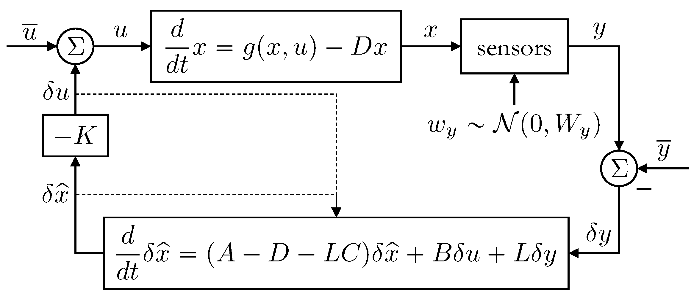
5. Linear Quadratic Gaussian (LQG) Control

This section describes the LQG strategies for state estimation and control and then discusses the observation models in construction.

5.1. LQG Controller

Precision is crucial in panel installation to prevent rework and minimize air leaks. However, achieving high-precision robotic panel installation under real-world conditions faces several challenges. The first challenge is that not all states are observable. Furthermore, not all observable states provide the desired update rate because of variations in processing time required for different sensor readings. The second challenge stems from the nature of outdoor applications, in which the system is inevitably affected by external disturbances such as wind or vibrations.

To address these challenges, we propose using an LQG controller for trajectory tracking, state estimation, and disturbance rejection. This would enable the CDPR to follow the desired trajectory and maintain the panel at the desired pose for a prolonged duration until the panel-fastening procedure is completed. The linear dynamics in Equation (8) are augmented with damping, process noise $w_x\sim \mathcal{N}(0,W_x)$, measurement noise $w_y\sim \mathcal{N}(0,W_y)$, and partial state observability:

$$\begin{array}{cc}\hfill {\displaystyle \frac{d}{dt}}\delta x& =(A-D)\delta x+B\delta u+w_x,\hfill \\ \hfill \delta y& =C\delta x+w_y,\hfill \end{array}$$

(26)

where C depends on the set of sensors used. Because the system is nonlinear, Equation (26) is applied at every point in the trajectory, resulting in a linear time-varying system. Figure 6 shows the control diagram.

5.2. Observations

The states include position, orientation, linear velocity, and angular velocity. In robotics, the position is often measured using cameras with fiducial markers, such as AprilTags or ArUco, or motion capture systems like VICON or OptiTrack. In construction, laser trackers are widely accessible and frequently used for highly precise angle, distance, and coordinate measurements. Thus, they are also valuable tools for position measurement. Among these options, laser trackers offer exceptional precision and high-frequency measurements. Motion capture systems also provide high precision and high frequency but lack scalability, requiring an increasing number of cameras as the construction site expands to maintain accuracy and coverage. Conversely, cameras with fiducial markers are the most cost-effective solution but suffer from lower accuracy and significantly reduced detection frequency. Given these considerations, in this study, we used laser trackers for position estimation.

Our previous work introduced the Real Time Evaluator (RTE), a tool specifically designed to measure the position and orientation of a panel using a laser tracker [33,34]. The RTE provides precise position measurements at a frequency of approximately 10–20 Hz, but it requires approximately 10 s for a single orientation measurement, as it must search for and measure three distinct targets. For our study, when using the RTE, we adopted a position measuring frequency of 10 Hz and an orientation measuring frequency of ${\displaystyle \raisebox{1ex}{$1$}\!\left/ \!\raisebox{-1ex}{$7$}\right.}$ Hz for observations. Considering that an IMU offers a higher measurement frequency and can provide both angular velocity and angles, we combined it with the RTE to measure orientation more quickly and to obtain extra angular velocity information. In this study, we considered only the angular measurements from the IMU because of the significant drift when integrating linear acceleration.

6. Simulation Results

Here, we first describe the implementation details for our simulations. We then analyze how the coefficients $\alpha$, $\beta$, and $\gamma$ in the cost function and initial orientation ${\mathbf{\Phi }}_0$ affected the optimal trajectories. Finally, we show that the LQG controller is able to estimate the panel state and mitigate the impact of external disturbances.

6.1. Implementation Details

We used a one-third-scaled model of a three-story residential building in our simulation. For all the experiments, we selected model 2 from Figure 3. CasADi [35] was employed as the numerical optimization solver with a sampling time of $\Delta t=t_T/N$. During implementation, we observed that adhering to the equality constraints from Equation (25) often made it challenging for the solver to converge. Therefore, we relaxed these hard constraints as follows:

$$\left[\begin{array}{c}-{ϵ}_F\\ -{ϵ}_M\end{array}\right]\le A_T^T{u}_T+w_{\mathrm{p}}\le \left[\begin{array}{c}{ϵ}_F\\ {ϵ}_M\end{array}\right].$$

(27)

Here, ${ϵ}_F$ and ${ϵ}_M$ are small positive numbers, allowing some slack on the force and moment balance, respectively. This relaxation had minimal impact on the stopping terminal constraint but significantly improved the convergence speed. The initial and terminal poses were defined based on the expected real-world scenario. The panel was picked up at the lower corner of the workspace ${\mathit{r}}_0={\left[\begin{array}{ccc}0.6& 0.8& 0.95\end{array}\right]}^T$ m with a predefined orientation and zero velocities. Then, the panel was held stationary at the final position ${\mathit{r}}_T={\left[\begin{array}{ccc}1.2& 2.74& 0.3\end{array}\right]}^T$ m, located at the top-right corner of the facade, with the panel fully plumb and level (${\mathbf{\Phi }}_T=0$). The model parameters and constraint specifications are listed in

Table 1. Model parameters and constraint specifications.

Variable	Value	Description
m	13.6 kg	Panel mass
$\mathit{F}$	${\left[\begin{array}{ccc}1.83& 3.12& 1.22\end{array}\right]}^T$ m	Frame dimensions
$\mathit{P}$	${\left[\begin{array}{ccc}0.76& 0.76& 0.25\end{array}\right]}^T$ m	Panel dimensions
${\mu }_{\mathit{v}}$	100	Linear friction coefficient
${\mu }_{\mathit{\omega }}$	3500	Angular friction coefficient
$f_{min}$	66 N	Cable sagging minimum force
$f_{max}$	1200 N	Cable rupture maximum force
${\mathbf{\Phi }}_{lim}$	20°	Euler angle orientation limit
${\mathit{v}}_{lim}$	0.2 m/s	Linear velocity limit
${\mathit{\omega }}_{lim}$	2 deg/s	Angular velocity limit
$t_T$	20 s	Terminal time
N	2000	Samples per trajectory
${ϵ}_F$	0.01	Force balance slack at $t_T$
${ϵ}_M$	0.0001	Moment balance slack at $t_T$
${\mathit{r}}_0$	${\left[\begin{array}{ccc}0.6& 0.8& 0.95\end{array}\right]}^T$	Panel pickup position
${\mathit{r}}_T$	${\left[\begin{array}{ccc}1.2& 2.74& 0.3\end{array}\right]}^T$	Panel final position

.

In practical applications, a CDPR system may encounter real-world challenges such as external wind disturbances, varying building geometries, and diverse anchor point configurations. In this study, we assume the CDPR frame to be a rectangular prism, which is a common and practical configuration for CDPRs and compatible with many building structures. External wind loads are modeled as impulse and sustained disturbances, which are intended to be handled by the proposed feedback controller. Variations in geometry and anchor placement are inherently addressed through the concept of the feasible workspace. Our prior work [2] has extensively studied the impact of different cable anchor configurations and wrench-feasible workspace, providing a strong foundation for the assumptions made in this study. These considerations contribute to the potential adaptability of the CDPR system in complex environments, and future work will further explore these aspects through physical implementation and testing.

6.2. Trajectory Optimization Results

This section examines how the choice of the coefficients $\alpha$, $\beta$, and $\gamma$ from Equation (15) affected the optimal force distribution.

6.2.1. Sensitivity of Control Effort

We tested different values of $\alpha$ ranging from 0.001 to 1. The initial orientation was set to ${\mathbf{\Phi }}_0=0$, assuming that the panel was picked up fully plumb and level. The optimal trajectories are illustrated on the right side of Figure 7. For the cases in which $\alpha <1$, the values $\beta =0.1$ and $\gamma =0$ were chosen to generate smooth trajectories. For the case in which $\alpha =1$, $\beta =\gamma =0$ allowed us to study the minimum effort control strategy. Figure 7 shows that, contrary to our intuition, the optimal trajectory did not correspond to a straight line between the initial and terminal positions. Instead, the optimal trajectory tended to bring the panel to the center of the frame before lifting it vertically to minimize the force needed using a simple hoisting strategy. When $\alpha =0.001$ (dashed line), the optimizer did not prioritize minimizing the overall force and focused only on generating a smooth trajectory. In this case, the trajectory approximated a straight line. As the value of $\alpha$ increased and the control input was further penalized, the optimal trajectories tended to move along the central vertical axis of the $xy$-plane. Note that when $\alpha =0.1$, the controller quickly moved the panel to the central vertical axis. Nonetheless, the trajectory remained smooth thanks to $\beta \ne 0$. When $\alpha =1$ and $\beta =\gamma =0$ (solid purple line), the optimal controller sought to minimize only the overall force. In this case, the trajectory generated was not smooth and changed sharply in direction. At the beginning of the trajectory, the controller used the gravitational force to move the panel to the central axis, thereby minimizing the force and energy spent. Although the panel needed to be lifted from a lower position, the simple hoisting movement along the vertical axis saved significant force. Finally, the controller performed a sharp movement at the top of the frame to position the panel at the desired pose.

6.2.2. Sensitivity of State Jerk

Figure 8 illustrates two optimal trajectories using $\alpha =0.001$, $\gamma =0$, and $\beta \gg \alpha$ in order to isolate as much as possible the effect of the state jerk penalty term. The average force exerted on a cable over the trajectory time span ($\overline{f}$) and the maximum cable force recorded ($f^{max}$) for each simulation are listed at the top. The optimal force distribution u had mostly similar characteristics for either case, reflected by the similarities in $\overline{f}$ and $f^{max}$. Note that the panel’s translational motion $\mathit{r}$ and the panel’s linear speed $\parallel \mathit{v}\parallel$ seem to have been independent of changes in $\beta$. However, this was not the case for the angular components. As $\beta$ increased, the range of orientation change (the difference between the maximum and minimum angles) reduced from 5° to 2°. Additionally, the range of the angular speed $\parallel \mathit{\omega }\parallel$ decreased from 1.2°/s to 0.3°/s. The average force on each cable increased from 140 to 160 N. Thus, a larger $\beta$ results in less aggressive rotational movement at the cost of requiring a slightly greater force on average. Note that, despite ${\mathbf{\Phi }}_0={\mathbf{\Phi }}_T=0$, the optimal controller rotated the panel during the trajectory. This indicates that inducing an appropriate level of rotation can reduce the average force needed to move the panel to the desired drop-off location.

6.2.3. Sensitivity of Force Jerk

Figure 9 shows the results with and without the force jerk in the cost function. Without a force jerk penalty ($\gamma =0$), the forces on two cables dropped by over 500 N within the first 0.5 s. Such aggressive changes could impose substantial stress on the winches that manipulate the cables. However, with a force jerk penalty, this rapid change in force was eliminated. The smoother trajectory came at the cost of a higher average force, as seen in the increase in $\overline{f}$ from 121 to 170 N. In addition, the rotational movement became less aggressive with the force jerk penalty in place. Therefore, incorporating both force jerk and state jerk penalties results in less aggressive rotational movements and smoother control at the cost of a higher force on average.

6.2.4. Sensitivity of Initial Panel Orientation

Figure 10 shows two solutions to the optimal control problem in which the only difference was the initial panel orientation ${\mathbf{\Phi }}_0$. In these solutions, the optimal trajectories differed significantly because the controller had to not only translate the panel to the desired drop-off location but also make the panel plumb and level at some point during the trajectory. Note that even though the case on the right had a nonzero initial orientation, the value of $f^{max}$ was lower than in the case in which ${\mathbf{\Phi }}_0=0$. This suggests that starting with a perfectly plumb and level panel at the pickup location may not be the most optimal approach. Thus, we formulated the following optimization to find the initial orientation that minimizes the force:

$$\begin{array}{cc}\hfill \underset{{\mathbf{\Phi }}_0}{min}{\parallel u_0\parallel }^2\mathrm{s}.\mathrm{t}.& 0=A_0^T{u}_0+w_{\mathrm{p}}\hfill \\ \hfill & -{\Phi }_{0,lim}\le {\mathbf{\Phi }}_0\le {\Phi }_{0,lim}.\hfill \end{array}$$

(28)

When the initial orientation limit was ${\Phi }_{0,lim}=10$°, the optimal initial orientations were ${\mathbf{\Phi }}_0={\left[\begin{array}{ccc}0.66°& 3.05°& -10°\end{array}\right]}^T$. Moreover, when ${\Phi }_{0,lim}=50°$, the optimal initial orientations were ${\mathbf{\Phi }}_0={\left[\begin{array}{ccc}-0.22°& 2.16°& -29.22°\end{array}\right]}^T$. Therefore, a large rotation around the $z^{\prime }$-axis can decrease the initial force needed to maintain the panel stationary. Figure 11 shows the optimal initial pose and the optimal trajectories. The initial pose in Figure 11a,b, although unconventional, satisfied wrench feasibility and avoided cable-to-cable and cable-to-panel collisions. Figure 11c shows how the optimal initial orientation ${\mathbf{\Phi }}_0$ changed as the panel pickup location moved along the x-axis. Note that the main contributor to ${\mathbf{\Phi }}_0$ was the rotation around the $z^{\prime }$-axis; the other rotations remained small to ensure wrench feasibility. The optimal trajectories depicted in Figure 11 had the lowest value of $f^{max}$ among all the simulations conducted. Also, note that the average force $\overline{f}$ was reduced compared with the simulations in Figure 10. Additionally, the profiles for linear and angular speeds were smooth and symmetric compared with previous results.

6.2.5. Discussion

In this section, we explored several optimal trajectories for automated panelized building envelope retrofits using CDPRs. The optimal trajectories were generated by formulating and numerically solving an optimal control problem. The cost function was designed to achieve minimum energy usage while maintaining smooth trajectories to transport a prefabricated panel from its initial pickup position to the target position. Minimum energy was achieved by minimizing the control effort, and trajectory smoothness was achieved by penalizing the state and control jerk. Such a formulation allows the system to favor more gradual and controlled motions, which leads to more predictable and stable CDPR behavior. Our experiments focused on understanding the sensitivity of various coefficients used in the cost function and examining how different initial orientations affect the force distribution of the cables.

The key findings are as follows:

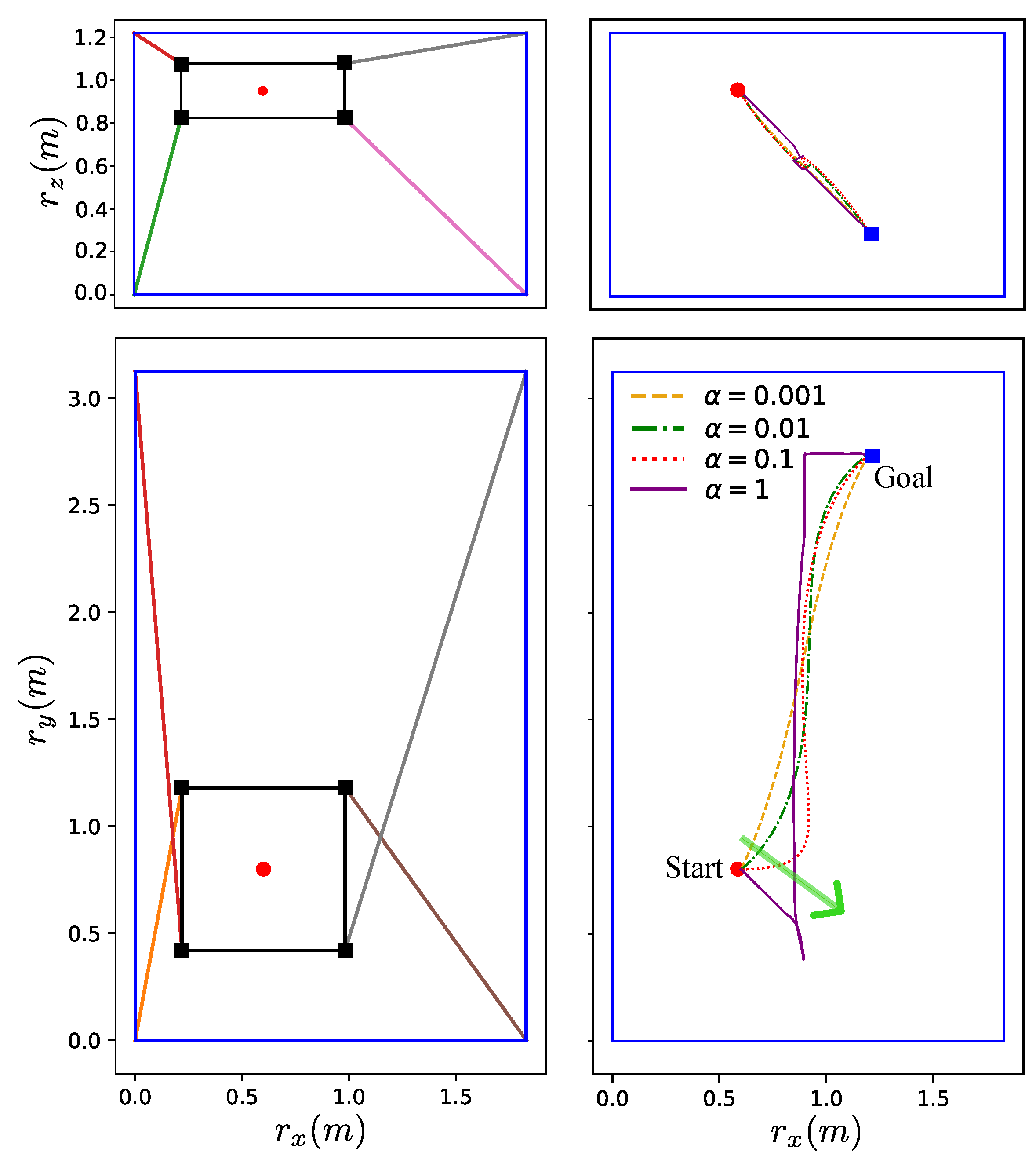
• Impact of increasing the force penalty: One of the main lessons learned from this study is that the more the force penalty increases, the more the trajectory resembles a vertical lift. When only the force penalty is considered in the cost function, the optimal trajectory initially uses gravity to bring the panel to the central vertical axis of the $xy$-plane. Then, the system lifts the panel straight up to a desired height before moving it horizontally to its final destination. This lift-like behavior highlights a key characteristic of a minimum-effort optimal controller: leveraging gravity to assist with horizontal displacement to minimize the force required during this process, followed by prioritizing the most energy-efficient vertical lift.
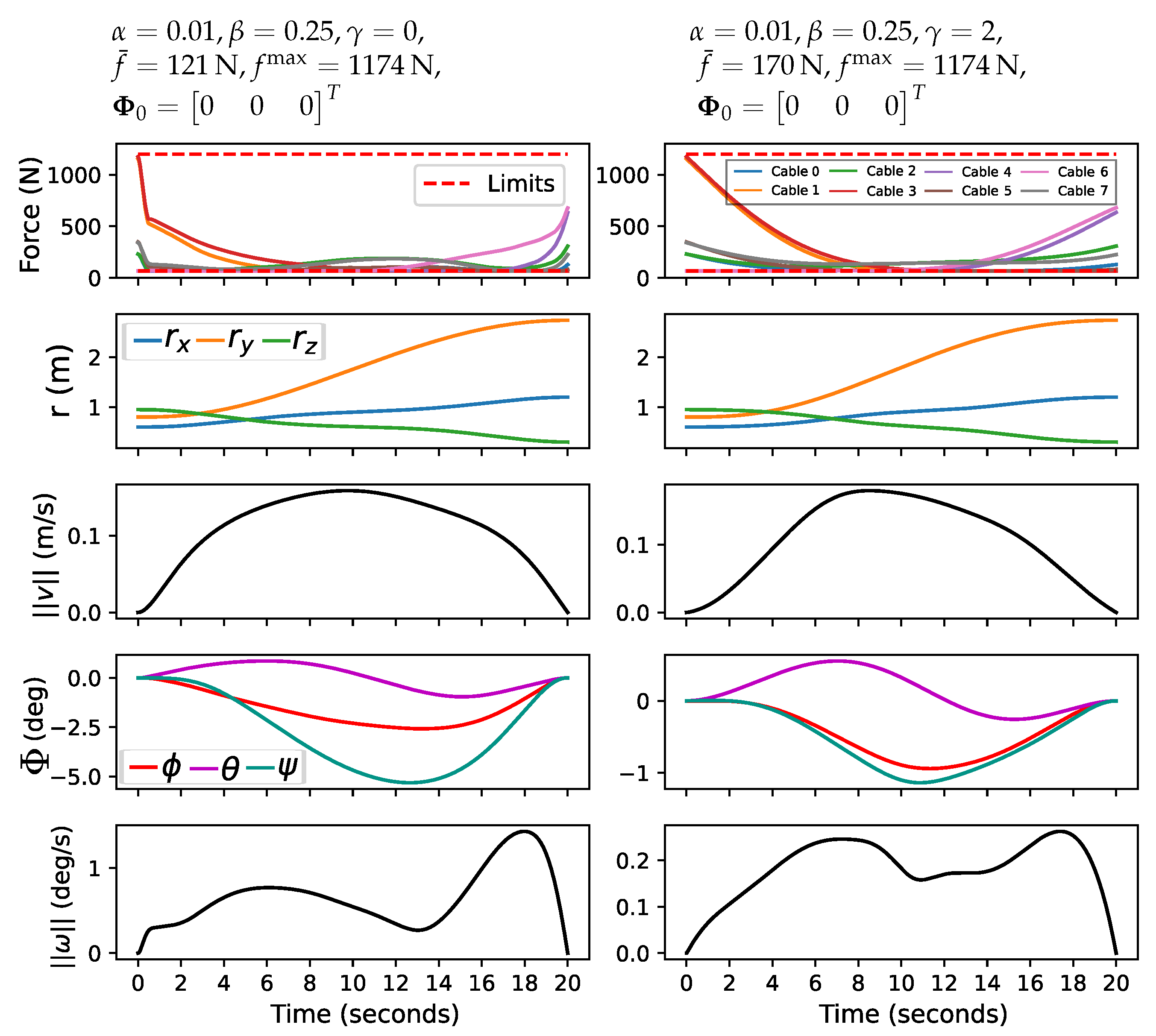
• Effect of the state jerk penalty: Our analysis indicates that increasing the state jerk penalty reduces the magnitude of rotational movement while maintaining smooth transitions. However, this comes with the cost of an increased average force.
• Effect of the force jerk penalty: Another critical finding relates to the force jerk and its impact on the actuator system. Although introducing the force jerk penalty slightly increases the average effort required, it can effectively reduce stress on the actuators by reducing sudden changes in control commands. This trade-off suggests that although the system may require marginally more energy, it operates more smoothly, which could lead to more reliable execution, extend the longevity of the actuators, and reduce maintenance needs.
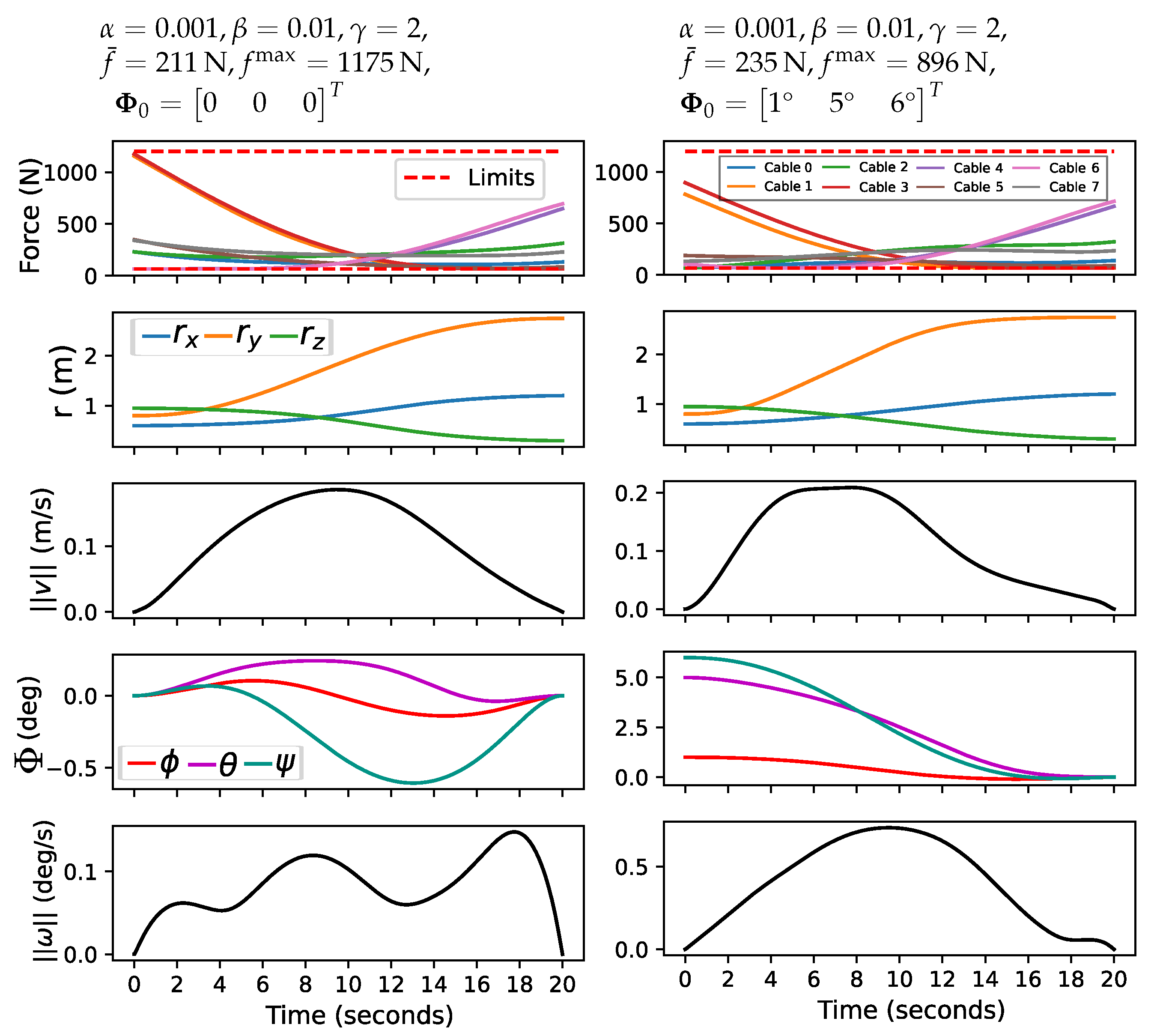
• Influence of initial orientation on force distribution: The simulation results show that the initial orientation of the panel plays an important role in determining how forces are allocated and managed at the beginning of the trajectory. Variations in initial orientation lead to different patterns of force distribution. This insight is particularly relevant for applications in which initial conditions are variable or difficult to control because it suggests that careful consideration of initial orientation can optimize force usage and overall system performance.
• Influence of trajectory orientation on force distribution: Even when the initial and terminal orientations are zero, the optimal trajectory still rotates the panel during the transition. The rotation acts as a mechanism to optimize the trajectory in a way that meets all the imposed constraints while minimizing the cost function. Even with zero initial and terminal orientations, allowing some degree of rotation during the transition can help distribute forces more evenly and reduce peak loads. Thus, the rotation effect during the trajectory reflects a complex trade-off aimed at achieving the most efficient overall motion profile, considering all aspects of the control objectives.

This section provides valuable insights into trajectory optimization for CDPRs in panelized building envelopes, focusing on minimum effort and smoothness criteria. By analyzing factors such as force penalties, state jerk penalties, force jerk penalties, and initial panel orientation, we deepen our understanding of how to formulate an optimal control problem that enables the efficient and reliable manipulation of prefabricated panels for automated construction tailored to specific operational requirements.

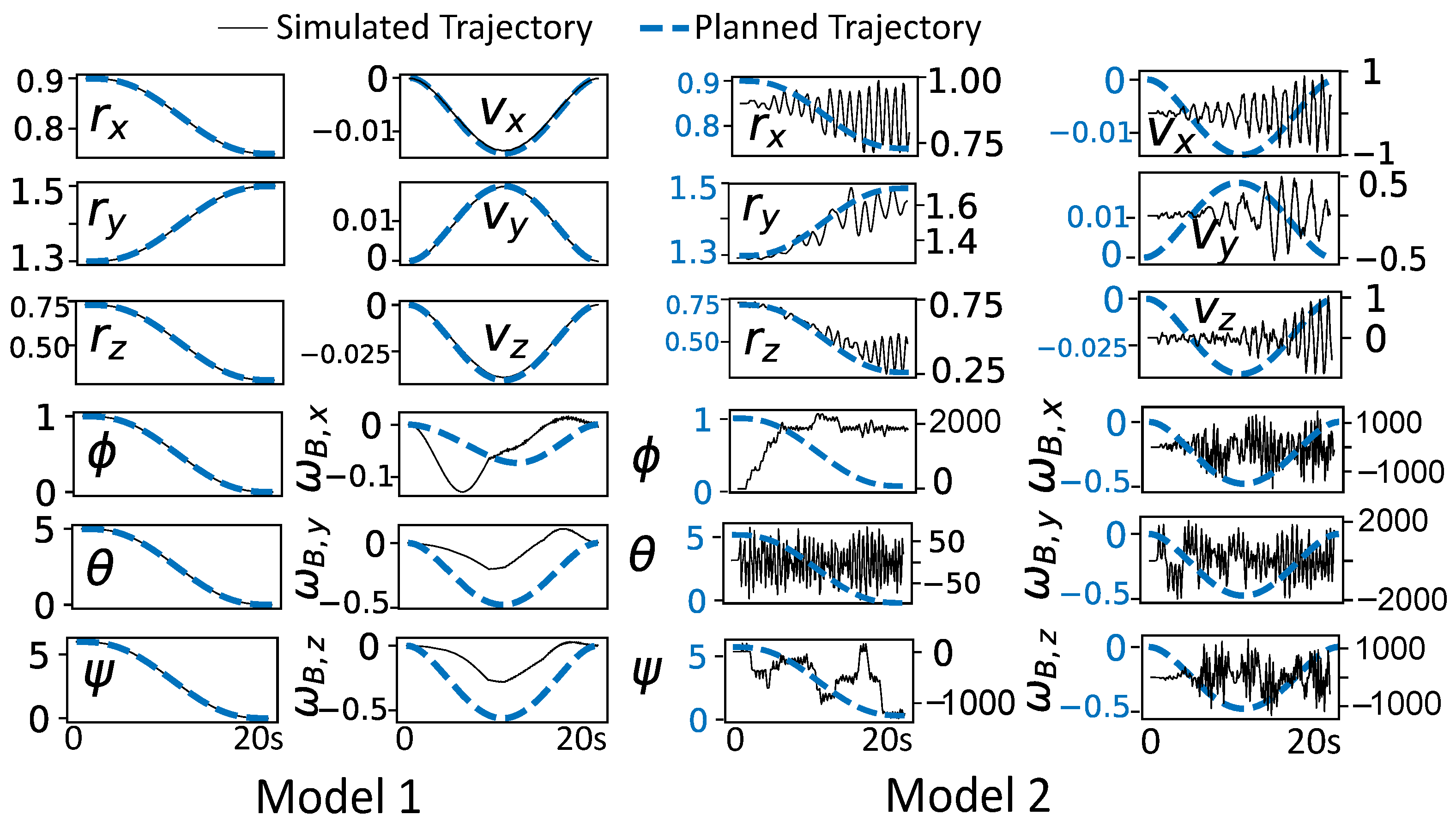
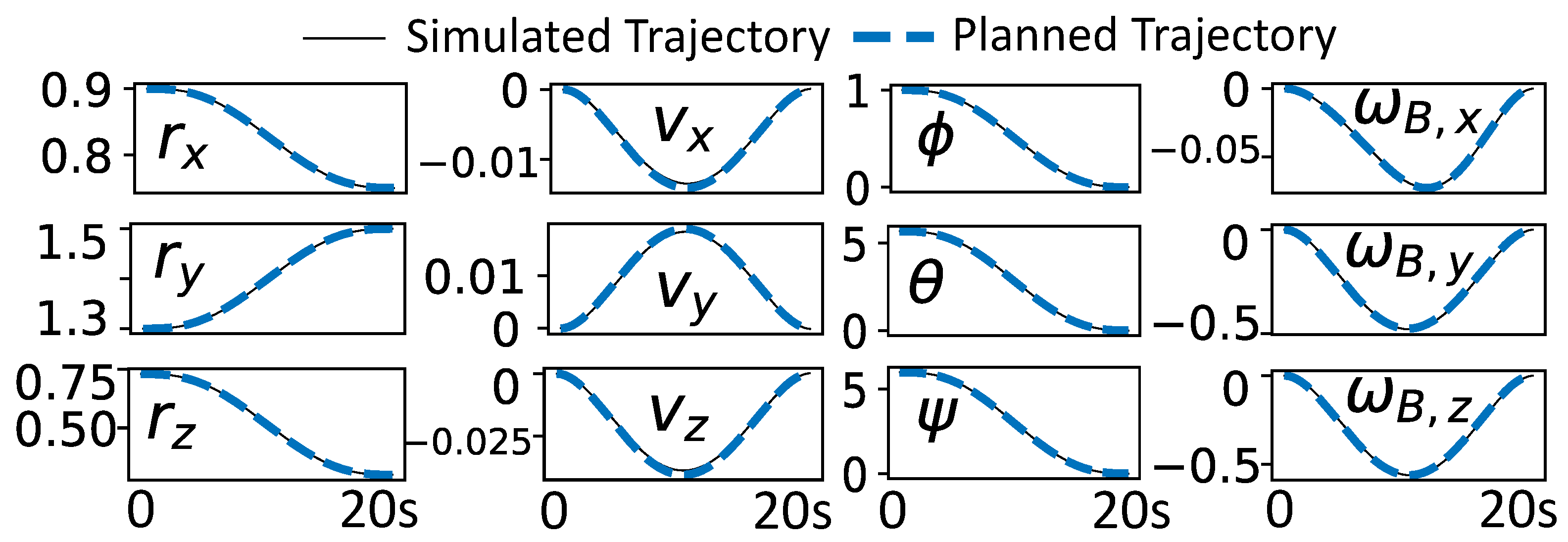
6.3. LQG Results

In our simulations, we examined the LQG controller using three types of observations.

Table 2. Three types of observations used in simulations. NA indicates states are not observable.

	r	$\mathbf{\Phi }$	v	${\mathit{\omega }}_{\mathcal{B}}$	Matrix C
RTE	10 Hz	${\displaystyle \raisebox{1ex}{$1$}\!\left/ \!\raisebox{-1ex}{$7$}\right.}$ Hz	NA	NA	diag $({\mathbb{E}}_6,0)$
RTE+IMU	10 Hz	10 Hz	NA	10 Hz	diag $({\mathbb{E}}_6,0,{\mathbb{E}}_3)$
Full state	10 Hz	10 Hz	10 Hz	10 Hz	${\mathbb{E}}_{12}$

describes the observability of the states and their corresponding frequencies according to the sensors used. The measurement noise, defined as $W_y=\mathrm{diag}(0.{003}^2{\mathbb{E}}_6,0.{002}^2{\mathbb{E}}_3,0.{001}^2{\mathbb{E}}_3)$, was consistent across all three observations. Similarly, the process noise was defined as $W_x=\mathrm{diag}(0.{003}^2{\mathbb{E}}_6,0.{002}^2{\mathbb{E}}_6)$. We conducted two sets of simulations. In the first set, we controlled the robot to track the predefined trajectory shown in the right plot of Figure 10, and the simulation lasted for 20 s. In the second set of simulations, we used a 50 s reference trajectory. For the first 20 s, the robot followed the same predefined trajectory, as shown in the right plot of Figure 10. During the remaining 30 s of the reference trajectory, the panel was expected to hold at the terminal (desired) state, which was implemented as a repetition of the final state and control input of the preplanned trajectory. Three different disturbances were introduced in this set. The first disturbance occurred only once, at the 3 s mark, and the second disturbance was applied as impulse signals at the 3, 5, and 6 s marks. Each disturbance affected the position $\mathit{r}$ by ${\left[\begin{array}{ccc}-5& 3& -2\end{array}\right]}^T$ mm, and the orientation $\mathbf{\Phi }$ was changed by ${\left[\begin{array}{ccc}-1.72°& -1.15°& 1.72°\end{array}\right]}^T$. The third type of disturbance is sustained signals, which cause the end effector to shift by ${\left[\begin{array}{ccc}-10& 6& -4\end{array}\right]}^T$ mm in position per second and ${\left[\begin{array}{ccc}-2.29°& -2.29°& -2.29°\end{array}\right]}^T$ in orientation per second. This disturbance persists for a duration of 5 s.

Table 3. Model 2 final state errors. ME denotes minimum effort LQR control, $t_s$ represents total simulation time, and $d_t$ indicates the time marks when disturbances are introduced.

${\mathit{d}}_{\mathit{t}}$	${\mathit{t}}_{\mathit{s}}$	Observations	${\mathit{e}}_{{\mathit{r}}_{\mathit{x}}}$ (mm)	${\mathit{e}}_{{\mathit{r}}_{\mathit{y}}}$	${\mathit{e}}_{{\mathit{r}}_{\mathit{z}}}$	${\mathit{e}}_{\mathit{\varphi }}$ (deg)	${\mathit{e}}_{\mathit{\theta }}$	${\mathit{e}}_{\mathit{\psi }}$	${\mathit{e}}_{{\mathit{v}}_{\mathit{x}}}$	${\mathit{e}}_{{\mathit{v}}_{\mathit{y}}}$	${\mathit{e}}_{{\mathit{v}}_{\mathit{z}}}$	${\mathit{e}}_{{\mathit{\omega }}_{\mathcal{B},\mathit{x}}}$	${\mathit{e}}_{{\mathit{\omega }}_{\mathcal{B},\mathit{y}}}$	${\mathit{e}}_{{\mathit{\omega }}_{\mathcal{B},\mathit{z}}}$
3 s	20 s	Feedforward	−16.367	−10.914	−44.314	−11.734	0.404	7.066	−1.770	−3.607	−6.558	−1.896	0.035	0.781
		RTE	−2.895	−3.101	−3.694	0.319	−0.134	−0.499	4.445	−9.679	−2.020	0.361	0.030	−0.267
3 s	20 s	RTE + IMU	−1.138	−1.789	−3.716	−0.294	−0.183	0.185	0.561	−4.777	0.585	0.052	0.024	−0.024
		Full state	−1.065	−1.822	−3.663	−0.278	−0.182	0.163	0.628	−4.858	0.926	0.048	0.024	−0.026
		RTE ME	−10.155	−37.155	−4.521	0.098	−0.150	0.361	4.955	−10.367	−1.634	0.396	0.031	−0.373
3 s	20 s	RTE + IMU ME	−3.183	−12.814	−3.873	−0.352	−0.196	0.440	1.153	−3.937	0.505	0.052	0.025	−0.047
		Full state ME	−3.108	−12.860	−3.929	−0.351	−0.195	0.429	1.481	−4.692	−0.336	0.059	0.025	−0.044
		RTE	0.680	−0.918	0.231	0.137	0.014	−0.306	0.847	1.829	1.254	0.043	−0.002	−0.023
3 s	50 s	RTE + IMU	−0.115	−0.019	0.021	−0.006	−0.002	0.012	0.062	−0.013	−0.083	0.002	0.001	0.000
		Full state	−0.028	0.115	0.133	0.002	−0.001	−0.003	0.285	−0.015	−0.459	−0.001	0.001	0.002
		RTE ME	−1.550	−7.458	−0.787	−0.084	0.030	0.021	0.997	3.286	0.144	0.038	−0.004	−0.070
3 s	50 s	RTE + IMU ME	−0.175	−0.225	−0.060	−0.014	−0.001	0.020	−0.084	−0.687	0.166	0.002	0.000	−0.001
		Full state ME	−0.157	0.207	0.136	0.004	−0.001	0.013	0.123	−0.145	−0.318	−0.003	0.001	−0.005
		RTE	−13.288	−3.441	−11.905	0.152	−0.513	−1.183	5.763	−11.776	1.002	0.947	0.139	−0.912
3, 5, 6 s	20 s	RTE + IMU	−7.036	−0.680	−11.874	−1.175	−0.627	0.732	5.087	−9.273	−1.727	0.188	0.106	−0.131
		Full state	−6.943	−0.707	−11.702	−1.149	−0.626	0.727	5.095	−9.179	−1.736	0.187	0.105	−0.127
		RTE	−1.978	−4.565	−3.228	−0.351	0.083	−0.156	2.789	0.984	0.565	0.074	−0.013	−0.185
3, 5, 6 s	50 s	RTE + IMU	−0.075	−0.069	−0.083	−0.015	−0.009	0.013	−0.245	0.294	0.271	0.002	0.001	0.002
		Full state	−0.080	0.049	0.028	−0.005	−0.007	0.011	−0.019	0.100	0.003	0.001	0.001	0.004
		RTE ME	−10.435	−17.273	0.513	−0.520	0.233	1.936	0.984	0.185	−4.596	−0.058	−0.018	−0.093
3, 5, 6 s	50 s	RTE + IMU ME	−0.342	−0.233	−0.100	−0.022	−0.007	0.048	0.031	−0.799	0.021	−0.002	0.001	−0.008
		Full state ME	−0.380	−0.118	0.077	−0.001	−0.006	0.050	−0.040	−0.513	−0.133	−0.002	0.001	−0.009
		RTE	−32.4	−230.3	57.6	2.816	0.588	2.711	2.295	98.480	−11.332	−0.344	0.028	0.143
Sustained	50 s	RTE + IMU	−0.270	−0.279	−0.439	−0.038	−0.025	0.044	−0.237	−0.040	0.365	0.006	0.003	−0.001
3 to 8 s		Full state	−0.240	−0.312	−0.361	−0.026	−0.025	0.022	−0.148	−0.241	−0.270	0.012	0.004	−0.005
3 to 8 s	80 s	RTE	1.598	−0.254	4.519	0.459	0.041	−0.228	−0.298	−1.035	0.705	−0.040	−0.002	0.115

presents the final state errors relative to the desired final state, where the desired position ${\mathit{r}}_T={\left[\begin{array}{ccc}1.2& 2.74& 0.3\end{array}\right]}^T$ and the desired orientation, linear velocity, and angular velocity are all zero. The first column categorizes the disturbance types, and the second column specifies the total simulation duration. The third column identifies the observation models used in each simulation. From the fourth column onward, the table displays the final state errors. We evaluated two different LQG controllers: a full LQR controller with different observation models and a minimum-effort LQR controller with different observation models. Additionally, force limits were enforced during the simulations (i.e., if the control inputs exceeded the allowable force range, they were projected back within the permissible limits). As shown in Table 3, feedforward commands led to significant errors in both position and orientation. Overall, the full LQR controller outperformed the minimum effort LQR controller, and as expected, full-state observation yielded significantly better results than RTE observation. When the RTE was augmented with IMU data, its performance closely approached that of full-state observation. The extended simulation time of 50 s, compared with 20 s, allowed the robot more time to settle and align with the desired final pose. When disturbances were applied three times, a 20 s simulation was insufficient for the robot to correct its pose fully, even under full-state observation. However, with a longer response time, such as a 50 s simulation, the final position errors for both full-state observation and RTE with IMU observation could be reduced to submillimeter levels for both the full LQR and minimum effort LQR controllers. In the case of the sustained disturbance, both the full state and RTE with IMU observations achieve submillimeter accuracy during a simulation duration of 50 s. However, the RTE observation results in significant errors. To address this, we extended the simulation time to 80 s, and the final errors were millimeter-level; see the last four rows in Table 3. Therefore, the simulation results demonstrate that the LQG controller effectively guides the end effector to recover from various types of disturbances, including single impulse, multiple impulses, and sustained disturbances, which satisfies the industry-standard 4 mm error tolerance. Even when using the RTE observation model, the controller is capable of correcting errors when sufficient simulation time is allowed.

Figure 12 compares the trajectories generated using the LQRs with three different observations. The arrows indicate when the impulse disturbances were applied. Two LQR feedback gains were simulated: full LQR and min effort LQR. The control gain K was calculated using $Q=\mathrm{diag}\left(\begin{array}{ccc}100{\mathbb{E}}_6,& {\mathbb{E}}_3,& 500{\mathbb{E}}_3\end{array}\right)$, and $R=0.001{\mathbb{E}}_8$ for the full LQR and using $Q=0$ and $R={\mathbb{E}}_8$ for the minimum effort LQR. Figure 12 shows that the LQR with RTE control exhibited oscillations, and certain states, such as ${\mathit{\omega }}_{\mathcal{B},z}$, failed to converge to the desired state on time.

To analyze the impact of the slow update rate of orientation measurements in RTE observation, we plotted the $\delta u$ and u trajectories in Figure 13. These force trajectories were generated using the full LQR with RTE observation and the full LQR with RTE observation augmented by IMU data. Because of the slow orientation update rate in RTE observation (e.g., one measurement every 7 s), the system exhibited a significant delay in responding to noise and disturbances. As a result, the final force trajectory was less smooth than the one generated by the RTE with an IMU, whose faster orientation update rate enabled a more responsive and stable control performance. Therefore, integrating higher-frequency orientation measurement sensors, such as IMUs, into the observation model is important to improve responsiveness and control performance.

Therefore, we conclude that feedforward control amplifies small disturbances, causing significant drift in both position and orientation. Though simulated results may not precisely replicate real-world conditions, they provide insights into potential drift accumulation over time, which necessitates a feedback controller. LQG controllers demonstrate remarkable performance by effectively confining position and orientation errors within a narrow range. Laser trackers provide high-precision position measurements, and incorporating IMU data for orientation measurement is crucial for improved accuracy and stability. Overall, these findings highlight the significance of the LQG strategy to mitigate drift and ensure accuracy in CDPRs for overclad prefabricated panel installation.

7. Conclusions and Future Development Plan

7.1. Conclusions

The construction industry needs to reduce costs, improve efficiency, and mitigate labor shortages. This simulation study demonstrates the feasibility of using CDPRs for panelized prefabricated building envelope retrofits, addressing key challenges in automation for the construction industry. Through dynamic modeling, trajectory optimization, and feedback control strategies, we showed that CDPRs can effectively handle heavy prefabricated panels in simulated construction environments. Our contributions included developing and analyzing a dynamic model for CDPRs, which highlights the critical role of damping; formulating a nonlinear programming-based trajectory optimization framework to generate efficient motion plans; and implementing an LQG control strategy to enhance trajectory tracking despite disturbances and partial observability. Additionally, we evaluated state estimation methods suited for construction settings, and we emphasized the importance of integrating high-frequency orientation measurements for improved trajectory tracking accuracy. The results demonstrate that CDPRs can achieve high-precision automation even in the presence of external wind disturbances, providing a foundation for future experimental validation and real-world deployment.

7.2. Future Development of a Real-World CDPR System

To transition from simulation to real-world deployment, we are developing a one-third-scale CDPR prototype modeled after a three-story residential building. This system will serve as a test bed for validating our trajectory optimization and control strategies under realistic conditions. The development process consists of several key phases.

System design and hardware integration. The prototype has been assembled with eight cables, a rigid frame and platform, and eight actuating systems equipped with torque sensors. These actuators control cable winding and unwinding through swivel pulleys. A human–machine interface enables manual control of individual servos and real-time monitoring of joint positions, torques, and other critical parameters. Network communications are set up. For state estimation, we have integrated an MS60 laser tracker and a wireless IMU, both communicating through a central network hub managed by a router. The primary framework is built on Python 3.8 and the Robot Operating System (ROS) Noetic.

Real-time control implementation. With our trajectory optimization framework now stable in simulation, the next step is to translate these control strategies to the real system for precise trajectory tracking. To achieve this, we take the following actions:

• Obtain the digital twin of the robot;
• Develop a dynamic model of the physical robot;
• Implement a PI-based torque controller to regulate cable forces;
• Deploy the LQG control strategy.

Experimental validation and performance evaluation. Once the hardware and control system are integrated, we will conduct extensive experimental tests to validate the accuracy and reliability of our approach. The experiments will focus on evaluating trajectory tracking performance, disturbance rejection capabilities, and energy efficiency. We will also compare real-world results with our simulated predictions to refine our models and improve overall system performance.

By following this structured development plan, we aim to bridge the gap between simulation and practical deployment, demonstrate the feasibility of using CDPRs in automated construction applications, and lay the foundation for future large-scale implementation.

References

- Salonvaara, M.; Aldykiewicz, A., Jr.; Hun, D.E.; Desjarlais, A.O. Cost Assessment of Building Envelope Retrofits; Technical Report; Oak Ridge National Lab.: Oak Ridge, TN, USA, 2020. [Google Scholar]
- Liu, Y.; Zhang, R.; Hayes, N.; Hun, D.E.; Maldonado Puente, B. Cable-Driven Parallel Robot (CDPR) for Panelized Envelope Retrofits: Feasible Workspace Analysis. In Proceedings of the International Symposium on Automation and Robotics in Construction, Lille, France, 3–5 June 2024; 2024; Volume 41, pp. 1081–1088. [Google Scholar]
- Pott, A.; Bruckmann, T. Cable-Driven Parallel Robots; Springer: Cham, Switzerland, 2013. [Google Scholar]
- Wu, Y.; Cheng, H.H.; Fingrut, A.; Crolla, K.; Yam, Y.; Lau, D. CU-brick cable-driven robot for automated construction of complex brick structures: From simulation to hardware realisation. In Proceedings of the 2018 IEEE International Conference on Simulation, Modeling, and Programming for Autonomous Robots (SIMPAR), Brisbane, Australia, 16–19 May 2018; pp. 166–173. [Google Scholar]
- Bruckmann, T.; Reichert, C.; Meik, M.; Lemmen, P.; Spengler, A.; Mattern, H.; König, M. Concept Studies of Automated Construction Using Cable-Driven Parallel Robots. In Cable-Driven Parallel Robots; Gosselin, C., Cardou, P., Bruckmann, T., Pott, A., Eds.; Springer: Cham, Switeland, 2018; pp. 364–375. [Google Scholar]
- Bosscher, P.; Williams, R.L.; Bryson, L.S.; Castro-Lacouture, D. Cable-suspended robotic contour crafting system. Autom. Constr. 2007, 17, 45–55. [Google Scholar] [CrossRef]
- Qian, S.; Li, C.; Zhao, Z.; Zi, B. Modeling and Experimental Validation of a Cable-Driven Robot for Three-Dimensional Printing Construction. J. Mech. Robot. 2025, 17, 061002. [Google Scholar] [CrossRef]
- Pott, A.; Meyer, C.; Verl, A. Large-scale assembly of solar power plants with parallel cable robots. In Proceedings of the ISR 2010 (41st International Symposium on Robotics) and ROBOTIK 2010 (6th German Conference on Robotics), Munich, Germany, 7–9 June 2010; VDE: Berlin, Germany, 2010; pp. 1–6. [Google Scholar]
- Murphy, K.; Soares, J.C.; Yim, J.K.; Nottage, D.; Soylemezoglu, A.; Ramos, J. Cooperative Modular Manipulation with Numerous Cable-Driven Robots for Assistive Construction and Gap Crossing. arXiv 2024, arXiv:2403.13124. [Google Scholar]
- Izard, J.B.; Gouttefarde, M.; Baradat, C.; Culla, D.; Sallé, D. Integration of a Parallel Cable-Driven Robot on an Existing Building Façade. In Cable-Driven Parallel Robots; Bruckmann, T., Pott, A., Eds.; Springer: Berlin/Heidelberg, Germany, 2013; pp. 149–164. [Google Scholar]
- Iturralde, K.; Feucht, M.; Illner, D.; Hu, R.; Pan, W.; Linner, T.; Bock, T.; Eskudero, I.; Rodriguez, M.; Gorrotxategi, J.; et al. Cable-driven parallel robot for curtain wall module installation. Autom. Constr. 2022, 138, 104235. [Google Scholar] [CrossRef]
- Badrikouhi, M.; Bamdad, M. Design, modelling, implementation, and trajectory planning of a 3-DOF cable driven parallel robot. Appl. Math. Model. 2024, 125, 210–229. [Google Scholar] [CrossRef]
- Bamdad, M. Time-energy optimal trajectory planning of cable-suspended manipulators. In Cable-Driven Parallel Robots; Springer: Berlin/Heidelberg, Germany, 2012; pp. 41–51. [Google Scholar]
- Hasan, M.; Haque, M.A.; Mominuzzaman, S.M.; Troyee, T.G. Optimization of CDPR Path Planning using a Branch and Bound Algorithm. In Proceedings of the 2023 6th International Conference on Electrical Information and Communication Technology (EICT), Khulna, Bangladesh, 7–9 December 2023; pp. 1–6. [Google Scholar]
- Rasheed, T.; Long, P.; Roos, A.S.; Caro, S. Optimization based trajectory planning of mobile cable-driven parallel robots. In Proceedings of the 2019 IEEE/RSJ International Conference on Intelligent Robots and Systems (IROS), Macau, China, 3–8 November 2019; pp. 6788–6793. [Google Scholar]
- Behzadipour, S.; Khajepour, A. Time-optimal trajectory planning in cable-based manipulators. IEEE Trans. Robot. 2006, 22, 559–563. [Google Scholar] [CrossRef]
- Qian, S.; Bao, K.; Zi, B.; Zhu, W. Dynamic trajectory planning for a three degrees-of-freedom cable-driven parallel robot using quintic B-splines. J. Mech. Des. 2020, 142, 073301. [Google Scholar] [CrossRef]
- Korayem, M.; Zehfroosh, A.; Tourajizadeh, H.; Manteghi, S. Optimal motion planning of non-linear dynamic systems in the presence of obstacles and moving boundaries using SDRE: Application on cable-suspended robot. Nonlinear Dyn. 2014, 76, 1423–1441. [Google Scholar] [CrossRef]
- Korayem, M.; Tourajizadeh, H.; Jalali, M.; Omidi, E. Optimal path planning of spatial cable robot using optimal sliding mode control. Int. J. Adv. Robot. Syst. 2012, 9, 168. [Google Scholar] [CrossRef]
- Santos, J.C.; Chemori, A.; Gouttefarde, M. Redundancy resolution integrated model predictive control of CDPRs: Concept, implementation and experiments. In Proceedings of the 2020 IEEE International Conference on Robotics and Automation (ICRA), Paris, France, 31 May–31 August 2020; pp. 3889–3895. [Google Scholar]
- Aflakian, A.; Safaryazdi, A.; Masouleh, M.T.; Kalhor, A. Experimental study on the kinematic control of a cable suspended parallel robot for object tracking purpose. Mechatronics 2018, 50, 160–176. [Google Scholar] [CrossRef]
- Le Nguyen, V.; Caverly, R.J. Cable-driven parallel robot pose estimation using extended Kalman filtering with inertial payload measurements. IEEE Robot. Autom. Lett. 2021, 6, 3615–3622. [Google Scholar] [CrossRef]
- Santos, J.C. Model Predictive Tracking Control of Cable-Driven Parallel Robots: From Concept to Real-Time Validation. Ph.D. Thesis, Université Montpellier, Montpellier, France, 2020. [Google Scholar]
- Chen, G.; Hutchinson, S.; Dellaert, F. Locally optimal estimation and control of cable driven parallel robots using time varying linear quadratic gaussian control. In Proceedings of the 2022 IEEE/RSJ International Conference on Intelligent Robots and Systems (IROS), Kyoto, Japan, 23–27 October 2022; pp. 7367–7374. [Google Scholar]
- Hibbeler, R.C. Engineering Mechanics Dynamics, 11th ed.; Pearson: Upper Saddle River, NJ, USA, 2007. [Google Scholar]
- McGhee, R.; Bachmann, E.R.; Zyda, M.J. Rigid Body Dynamics, Inertial Reference Frames, and Graphics Coordinate Systems: A Resolution of Conflicting Conventions and Terminology; Naval Postgraduate School: Monterey, CA, USA, 2000. [Google Scholar]
- Mamidi, T.K.; Bandyopadhyay, S. Forward dynamic analyses of cable-driven parallel robots with constant input with applications to their kinetostatic problems. Mech. Mach. Theory 2021, 163, 104381. [Google Scholar] [CrossRef]
- Miermeister, P.; Pott, A. Modelling and real-time dynamic simulation of the cable-driven parallel robot IPAnema. In New Trends in Mechanism Science: Analysis and Design; Springer: Dordrecht, The Netherlands, 2010; pp. 353–360. [Google Scholar]
- Zi, B.; Duan, B.; Du, J.; Bao, H. Dynamic modeling and active control of a cable-suspended parallel robot. Mechatronics 2008, 18, 1–12. [Google Scholar] [CrossRef]
- Lamaury, J.; Gouttefarde, M. Control of a large redundantly actuated cable-suspended parallel robot. In Proceedings of the 2013 IEEE International Conference on Robotics and Automation, Karlsruhe, Germany, 6–10 May 2013; pp. 4659–4664. [Google Scholar]
- Sheng, Z.; Park, J.H.; Stegall, P.; Agrawal, S.K. Analytic determination of wrench closure workspace of spatial cable driven parallel mechanisms. In Proceedings of the International Design Engineering Technical Conferences and Computers and Information in Engineering Conference, Boston, MA, USA, 2–5 August 2015; American Society of Mechanical Engineers: New York City, NY, USA, 2015; Volume 57144. [Google Scholar]
- Ratiu, M.; Prichici, M.A. Industrial robot trajectory optimization-a review. In MATEC Web of Conferences; EDP Sciences: Les Ulis, France, 2017; Volume 126, p. 02005. [Google Scholar]
- Hayes, N.W.; Maldonado, B.P.; Hun, D.; Wang, P. Real-time evaluator to optimize and automate crane installation of prefabricated components. In Proceedings of the 40th International Symposium on Automation and Robotics in Construction, Chennai, India, 3–9 July 2023; pp. 192–199. [Google Scholar] [CrossRef]
- Tang, M.; Hayes, N.; Maldonado Puente, B.; Hun, D.E. Component Pose Reconstruction Using a Single Robotic Total Station for Panelized Building Envelopes; Technical Report; Oak Ridge National Laboratory (ORNL): Oak Ridge, TN, USA, 2024. [Google Scholar]
- Andersson, J.A.E.; Gillis, J.; Horn, G.; Rawlings, J.B.; Diehl, M. CasADi—A software framework for nonlinear optimization and optimal control. Math. Program. Comput. 2019, 11, 1–36. [Google Scholar] [CrossRef]