Abstract
The rapid measurement of three-dimensional bridge geometric shapes is crucial for assessing construction quality and in-service structural conditions. Existing geometric shape measurement methods predominantly rely on traditional surveying instruments, which suffer from low efficiency and are limited to sparse point sampling. This study proposes a novel framework that utilizes an airborne LiDAR–camera fusion system for data acquisition, reconstructs high-precision 3D bridge models through real-time mapping, and automatically extracts structural geometric shapes using deep learning. The main contributions include the following: (1) A synchronized LiDAR–camera fusion system integrated with an unmanned aerial vehicle (UAV) and a microprocessor was developed, enabling the flexible and large-scale acquisition of bridge images and point clouds; (2) A multi-sensor fusion mapping method coupling visual-inertial odometry (VIO) and Li-DAR-inertial odometry (LIO) was implemented to construct 3D bridge point clouds in real time robustly; and (3) An instance segmentation network-based approach was proposed to detect key structural components in images, with detected geometric shapes projected from image coordinates to 3D space using LiDAR–camera calibration parameters, addressing challenges in automated large-scale point cloud analysis. The proposed method was validated through geometric shape measurements on a concrete arch bridge. The results demonstrate that compared to the oblique photogrammetry method, the proposed approach reduces errors by 77.13%, while its detection time accounts for 4.18% of that required by a stationary laser scanner and 0.29% of that needed for oblique photogrammetry.
1. Introduction
The measurement of bridge geometric shape is one of the key contents throughout the entire life cycle of a bridge, including the construction phase, the load test process, and the service phase. However, bridge structures are generally characterized by large spans and high heights, which pose a serious challenge to the fast and accurate measurement of their geometric shape. Existing geometric shape measurement methods rely on the manual operation of a total station to measure point by point. This kind of method is simple and reliable, and the error can be controlled within centimeters when measuring kilometer-level bridges. However, it has the disadvantage of relying on the manual pre-laying of reflecting prisms, which is dangerous and time-consuming when measuring the geometric shape of large-span bridges. Additionally, this point-by-point method can only measure a small number of points and, therefore, may fail to monitor the deformation of some locations where no measurement points have been arranged.
Non-contact measurement methods, such as vision-based methods and radar-based methods, have been rapidly developed in recent years, providing efficiency and accuracy improvements for bridge inspection, and these methods have been extensively applied to the surface defect detection of bridges [1], the deformation measurement of bridges [2], the tension detection of cables [3], and the 3D model reconstruction of bridges [4]. However, as revealed by algorithmic principles, such deformation monitoring methods yield temporal variations in bridge morphology rather than quantifying absolute geometric states. The prerequisite for measuring 3D bridge geometric shapes lies in acquiring high-fidelity 3D point cloud representations of the structure. Commonly used techniques for acquiring 3D point clouds include stereo vision-based methods [5], structured light-based methods [6], laser scanning-based methods [7], and millimeter-wave radar-based methods [8]. The equipment for acquiring 3D information includes UAVs equipped with mapping cameras, stereo vision scanners, structured light scanners, 3D Light Laser Detection and Ranging (LiDAR), and millimeter-wave radar systems [9,10]. Among them, the point cloud density generally acquired by millimeter-wave radar is quite sparse, so it is usually not used in the dense 3D reconstruction of large scenes. Three-dimensional scanners based on the stereo vision principle or based on the structured light principle are generally characterized by a short baseline, high accuracy, and a high frame rate, but they can generally only be used for high-precision small-volume 3D scanning in indoor environments [11]. Multi-view image 3D reconstruction based on an unmanned airborne camera is a 3D reconstruction method widely used in structural inspection. The cost of this method is much lower than that of other methods. Still, the reconstruction accuracy of this method is affected by a variety of factors, such as the quality of the camera, the lighting situation, the shadow occlusion, and the overlap rate of the image. The accuracy of the large-scale 3D reconstruction can hardly reach the centimeter level, and the reconstruction algorithms can be extremely time-consuming [4].
Three-dimensional laser scanning has the characteristics of rapidity, non-contact, active point cloud acquisition, high density, and high accuracy of point cloud quality. The two main types of scanning are static Terrestrial Laser Scanning (TLS) and mobile dynamic scanning. For a static TLS implementation, multiple scanning stations must be strategically installed around the bridge peripheries and deck surfaces. Each station conducts localized scanning, subsequently registering all station-specific datasets into a unified point cloud. This methodology necessitates over 30 scanning stations for long-span bridges, resulting in prolonged field operations. Post-acquisition workflows demand labor-intensive or automated point cloud registration processes, significantly increasing temporal costs. For instance, Lin et al. [12] implemented TLS for bridge scanning, reporting 3 h of scanning for the bridge, and the point cloud density of the bridge reached 7700 points per square meter. For large-scale bridge point cloud data acquisition, two primary scanning methods exist due to the classification of 3D laser scanning into stationary static scanning and mobile dynamic scanning. In static scanning, multiple measurement stations are established around and on the bridge deck, with scanning performed at each station, followed by data stitching. Long-span linear bridges typically require setting up over 30 stations, resulting in a time-consuming process. Lu et al. proposed a top-down scanning strategy tested on over 10 highway bridges, showing an average scanning time of 2.8 h across 17 scanning sessions [13]. Mohammadi et al. utilized TLS to scan Werrington Bridge, obtaining 525 million points requiring approximately 15 GB of storage space [14]. Post-scanning, manual or automated point cloud registration is needed to align point clouds from all stations, a process that remains labor-intensive. While automated registration methods have emerged, such as Shao et al. proposed a marker-free approach using structured light scanners (SLSs) and TLS point clouds, which replaces marker-based coarse registration with an iterative closest point (ICP) algorithm to refine alignment, reducing per-station registration time to 2 min [15]. However, existing methods often depend on additional sensors or targets and face limitations in processing massive point clouds [16]. In recent years, growing applications of vehicle-mounted [17], UAV-borne [18], and handheld [19] laser scanners have been seen in dynamic scanning. These mobile platforms equipped with LiDAR can reconstruct bridges by flying predefined routes over the structure, using inertial navigation systems (INS) and GPS data to calculate trajectory and stitch temporal point clouds. For instance, Zhu et al. investigated UAV-based LiDAR-RGB fusion for bridge reconstruction, demonstrating its capacity to provide precise spatial information, though it requires post-processing for point cloud alignment [20]. Li et al. achieved a high-precision bridge model (overall accuracy: 1.70 cm) by fusing UAV imagery with TLS point clouds [21]. While dynamic scanning significantly reduces field time, post-processing alignment remains crucial, particularly for INS-based systems where positioning errors degrade reconstruction accuracy. For example, INS-estimated UAV positions typically accumulate substantial errors, leading to reduced model fidelity. Therefore, developing efficient and robust laser scanning equipment specifically for bridges, along with advanced point cloud registration methodologies, constitutes an essential research direction.
After obtaining the 3D point cloud of bridges, how to rapidly and automatically extract the linear alignment of key bridge components from massive 3D point clouds becomes a critical focus. Huang et al. proposed a power line detection method utilizing UAV LiDAR edge computing and 4G real-time transmission. This approach first employs semantic feature constraints to classify laser points in power line corridors into ground, vegetation, towers, cables, and building types, followed by trained deep learning models to further identify tower types for strain span separation [22]. The second challenge involves segmenting component-specific point clouds from bridge point clouds. For instance, extracting the point cloud of cable clamps and deriving their central coordinates enables the acquisition of cable linear alignment. Xu et al. developed a deep learning pre-segmentation method for bridge 3D reconstruction to detect cable alignment. Their methodology first applies deep learning-based object detection combined with Euclidean clustering to generate cropped sub-image sets of cable clamps automatically, then employs a 3D-to-2D grid projection-based image mask generation technique to retain valid pixels for camera pose estimation [23]. Kim et al. proposed a similar approach for segmenting bridge piers and girders, initially performing deep learning segmentation on 3D reconstruction images before projecting the segmentation results onto image-based reconstructed 3D point clouds [24]. Regarding point cloud segmentation from LiDAR data, Xia et al. presented a method combining local descriptors with machine learning for automatic detection of bridge structural components. Based on bridge geometric features, they designed a multi-scale local descriptor for training a deep classification neural network, achieving 97.26% accuracy in concrete girder bridge tests [25]. Yang et al. developed a weighted superpoint graph (WSPG) method for direct component recognition from large-scale bridge point clouds. The bridge point cloud is first clustered into hundreds of semantically homogeneous superpoints, then classified into different bridge components using PointNet and graph neural networks, attaining 99.43% accuracy in both real and synthetic datasets [26]. Jing et al. proposed BridgeNet, a 3D deep learning neural network for automatic segmentation of masonry arch bridges, achieving a maximum mean intersection-over-union of 94.2% in synthetic dataset training and testing [27].
While these studies demonstrate that deep learning-based point cloud segmentation methods can achieve satisfactory accuracy, current research encounters two significant limitations. First, most studies rely on synthetic datasets due to data scarcity, with each dataset containing only thousands of bridge point clouds, significantly fewer than the hundreds of millions of points in real LiDAR-acquired bridge point clouds. Second, the computational efficiency of algorithms remains insufficiently addressed. Practical applications reveal that processing bridge point clouds containing tens of millions of points using 3D deep learning methods imposes enormous demands on Graphics Processing Unit (GPU) memory. Even processing bridge point clouds with less than 1.4 million points requires over 30 min. Therefore, developing algorithms with lower computational demands and higher efficiency for processing large-scale real bridge point clouds remains another critical research challenge.
Based on the above review, this study proposes an integrated camera–LiDAR fusion framework for rapid 3D bridge reconstruction and a point cloud segmentation method for bridge components to efficiently measure bridge geometric linearity. The methodology centers on three contributions: (1) A multi-sensor acquisition system integrating LiDAR, cameras, and an inertial measurement unit (IMU) is developed, featuring an embedded real-time reconstruction processor designed for UAV deployment to perform dynamic large-scale scanning. (2) A coupled visual-LiDAR odometry Simultaneous Localization and Mapping (SLAM) algorithm is implemented to synchronously process point cloud and image data during dynamic scanning, enabling real-time point cloud stitching and visualization. (3) A deep learning segmentation method based on image-point cloud feature matching is proposed to automatically extract bridge components from reconstructed point clouds, allowing for the rapid geometric measurement of structural elements.
The remainder of this study is structured as follows: The general framework of the proposed LiDAR camera fusion-based geometric shape measurement method for bridges is presented in Section 2. The designed system is presented in Section 3. Section 4 introduces the 3D reconstruction methods based on LiDAR and camera fusion, and the proposed method is verified by field-testing a bridge in Section 5. Section 6 describes the conclusions of this work.
2. Framework of the Proposed Method
The core of the proposed method is to develop a LIDAR, camera, and IMU fusion system to rapidly and dynamically reconstruct a 3D point cloud of the bridge. A learning-based image segmentation network is proposed to automatically extract key components of the bridge from the point cloud based on the matching relationship between the camera and LiDAR. The 3D line shape of the components can be extracted, as shown in Figure 1. Based on this, the proposed method can be divided into three parts: establishing a multi-sensor fusion data acquisition system, the mapping method based on image and laser point cloud fusion, and the point cloud extraction method for bridge components based on image segmentation.
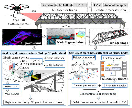
Figure 1.
Framework of the proposed method.
The first part addresses two fundamental technical challenges: temporal synchronization within multi-sensor fusion systems and comprehensive system calibration. Temporal synchronization is achieved through a GNSS (Global Navigation Satellite System)-synchronized processing unit that timestamps camera and LiDAR data streams, followed by the temporal alignment of multi-sensor measurements based on their respective sampling rates. The calibration process encompasses three essential procedures: (1) intrinsic camera calibration for lens distortion correction, (2) LiDAR-IMU calibration to compensate for motion-induced point cloud distortions during dynamic operations, and (3) cross-sensor calibration to determine precise extrinsic parameters between the camera and LiDAR systems. Only after completing these synchronization and calibration protocols can the acquired multi-modal data be effectively utilized for subsequent sensor fusion and high-precision mapping operations.
The second part focuses on reconstructing bridge 3D point clouds using preprocessed sensor data. This approach distinguishes itself from conventional LiDAR-based mapping methodologies through the implementation of a dual-odometry framework that synergistically combines VIO and LIO. A tightly coupled fusion framework is developed to integrate pose estimation outcomes from both modalities, effectively capitalizing on the complementary advantages of visual data’s dense feature representation in proximate ranges and LiDAR point clouds’ superior spatial constraint accuracy at extended distances. This hybrid architecture significantly enhances system robustness in 6-Degrees of Freedom (DoF) pose estimation and enables the generation of globally consistent 3D point cloud models.
The third part focuses on automatically identifying bridge components from collected bridge images, segmenting these elements, and restoring their 2D coordinates to the global 3D coordinate system of the bridge through image–point cloud alignment. Specifically, a deep learning-based image segmentation technique is first proposed to automatically segment bridge joints from the massive images acquired in the initial phase. Subsequently, the spatial correspondence between each image and its associated laser point cloud data are utilized to derive the 3D point cloud representation of each segmented part. The 3D coordinates of the components are then extracted from their corresponding point clouds. By integrating all detected component coordinates through this workflow, the geometric shape configuration of the entire bridge structure is reconstructed.
3. Establishment of LiDAR–Camera Fusion Measurement System
As a commonly used measurement device, cameras have undergone significant development and reached maturity. Therefore, this study employs an industrial camera as the image acquisition sensor. Meanwhile, LiDAR, as a precision measurement sensor, has traditionally been characterized by high costs; some stationary high-precision LiDAR scanners exceed hundreds of thousands of US dollars, while handheld dynamic laser scanners typically cost tens of thousands of dollars. With the rapid development of autonomous driving technology in recent years, low-cost sensor-grade LiDARs have been developed, making the widespread application of LiDAR feasible. Notably, the Livox series LiDARs are priced at only a few hundred dollars, yet their non-repetitive scanning pattern enables point cloud density comparable to more expensive scanners during low-speed mobile scanning. Based on these advantages, this research adopted the Livox LiDAR as the scanning sensor in a low-cost scanning system.
Specifically, the industrial camera employed is the HIKROBOT MV-CE120-10UC equipped with a 5 mm focal-length lens, capable of capturing images at 4000 × 3036 pixel resolution. The LiDAR unit selected is the Livox Avia, featuring a scanning range exceeding 190 m, point cloud density of 240,000 points/second, and an integrated BMI088 IMU with 0.09 mg resolution. The system also incorporates a processing unit for point cloud and image storage and processing. The processor used in this study is the Intel NUC12, configured with an i5-12500H CPU, 16 GB of Random Access Memory (RAM), and 256 GB of storage.
To minimize the weight of the system and make it easy to mount on the UAV, the aforementioned LiDAR and camera were connected together by a 3D-printed frame. The processor used for data analysis is placed in the lower part of the UAV to balance the center of gravity of the UAV. The UAV equipped with the complete system is the M300 RTK UAV from DJI Company, Shen Zhen, China, which can provide about 35 min of flight time. The complete data acquisition system is shown in Figure 2.

Figure 2.
The developed unmanned airborne LiDAR camera fusion system.
Sensor calibration is the basic work before measurement, and the proposed method includes three kinds of sensors: LiDAR, camera, and IMU, so each sensor needs to be calibrated separately first. For digital cameras, a variety of calibration methods can be used to calibrate the camera, depending on different camera models and different calibrators. Among them, Zhang’s calibration method is one of the most commonly used calibration methods, and in this part, Zhang’s calibration method is adopted to calibrate the intrinsic parameter matrix of the camera.
Regarding LiDAR calibration, since the 3D reconstruction in this study involves dynamic scenarios where the UAV maintains continuous motion during laser scanning, the following challenge arises: As the LiDAR collects each segment of point cloud data, it must accumulate laser returns over a specific time interval. During this interval, the UAV’s movement causes shifts in the coordinate system of points within each point cloud frame, resulting in distortion. To address this, motion-induced distortion in the LiDAR data must be eliminated through calibration between the LiDAR and the IMU prior to measurement.
Unlike conventional rotating mechanical LiDAR systems, the Livox LiDAR adopted in this research utilizes a semi-solid-state design incorporating a rotating prism mechanism. This configuration projects laser beams through precisely coordinated rotations of multiple prisms, generating a predetermined scanning trajectory. While significantly more cost-effective than traditional rotating mechanical LiDARs, its scanning mechanism fundamentally differs through the implementation of non-repetitive scanning patterns. The non-repetitive scanning achieves progressive field-of-view (FOV) coverage proportional to integration duration. At an integration time of 100 ms, the point cloud coverage approximates that of a conventional 32-beam LiDAR. Furthermore, the Livox Avia scanner exhibits a distinctive flower-petal-shaped scanning trajectory during operation, as illustrated in Figure 3a. Figure 3b demonstrates point cloud distortions induced by rotational and translational motions. During operation, the LiDAR operates at a standard sampling frequency of 10 Hz, corresponding to a 100 ms interval for laser emission and reception. When divided into three temporal segments (T1, T2, T3), the following effects are observed: During the first temporal segment (T1) with static LiDAR conditions, point cloud data are acquired at positions a1–c1. In the second segment (T2) under rotational motion, sampling positions shift to a2–c2. During the third segment (T3) involving translational motion, sampling positions further shift to a3–c3.
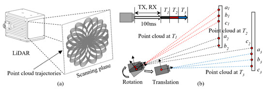
Figure 3.
(a) Trajectory of the point cloud and (b) the onset of motion blur in point clouds.
Motion distortion correction requires transforming the coordinates of each point within a LiDAR frame to their corresponding LiDAR origin at respective timestamps. Under minimal motion conditions, adjacent points demonstrate sufficient spatial continuity and overlap, enabling the application of point cloud registration-based estimation methods. These methods typically utilize the Iterative Closest Point (ICP) algorithm or its derivatives to compute inter-frame transformations for point cloud alignment [28]. However, such approaches inherently assume constant velocity motion and yield approximate solutions, leading to cumulative errors during extended scanning sessions. An alternative methodology integrates IMU data to estimate LiDAR motion states. By fusing high-frequency local pose estimations with kinematic state calculations, this approach reconstructs the LiDAR’s instantaneous orientation and velocity during data acquisition, enabling precise point cloud reprojection.
We assume the motion state of the LiDAR during scanning is represented as , where R denotes the rotation matrix, P is the position vector, V represents the velocity, and b corresponds to the accelerometer bias. Let the world coordinate system be denoted as W and the LiDAR coordinate system as B. To analyze the LiDAR’s motion using IMU data, the objective reduces to solving R, P, and V. In the implemented hardware configuration, the IMU operates at a data acquisition frequency of 200 Hz, while the LiDAR operates at 10 Hz. To correct LiDAR point cloud distortion using IMU data, the IMU measurements must first undergo integration. The angular velocity and acceleration from the IMU are defined as
where and represent the angular velocity and acceleration measured by the IMU at time t, denotes the true angular velocity, and , , , and correspond to the biases and noise in the measurements. The rotation matrix transforms coordinates from the world frame W to the LiDAR frame B, and g is the gravitational acceleration vector. Based on kinematic relationships among displacement, velocity, and acceleration, the position vector, velocity, and accelerometer bias from time t to t + Δt can be expressed as
Applying the inertial pre-integration method, the change in velocity, position, and rotation matrices from time i to time j can be expressed as
After obtaining the position and attitude transformation matrices of the system using the above equations, the point clouds during an acquisition time period (T1–T3) can be transformed to a coordinate system.
Following the calibration of the LiDAR-IMU system, the extrinsic matrix between the LiDAR and camera must be determined to establish spatiotemporal correspondence between image frames and 3D point clouds. Temporal synchronization across multi-sensor systems forms the foundation of sensor fusion methodologies. In this study, the LiDAR’s integrated IMU inherently ensures synchronization between the IMU and LiDAR, enabling simultaneous data acquisition through the direct invocation of the LiDAR driver. However, the camera and LiDAR operate as independent acquisition units, necessitating explicit temporal alignment between image frames and point cloud sequences prior to calibration and fusion.
The synchronization challenge between LiDAR and camera encompasses two aspects: clock synchronization and data acquisition synchronization. For clock synchronization, a common solution involves integrating a GPS into the acquisition system, where the GPS timing signal is fed to the central processing unit to unify timestamps. Regarding data acquisition synchronization, multiple approaches exist depending on synchronization precision requirements. A simplified method employs software-based triggering by initiating both sensors through a unified software command. For instance, if both LiDAR and camera operate at 10 Hz, their acquisition cycles theoretically align. However, this software-triggered approach suffers from inherent limitations: neither sensor strictly adheres to the nominal 10 Hz frequency due to timing jitter, causing progressive temporal misalignment during prolonged operation. While negligible for short-duration acquisitions, cumulative errors become significant over extended periods. A more robust solution utilizes external hardware triggering. This method applies to sensors supporting external trigger modes, where a dedicated device generates synchronization signals. The LiDAR and camera initiate acquisition upon receiving these signals, reducing inter-sensor synchronization errors to approximately 10 ms. In this study, the Livox Avia LiDAR supports Pulse Per Second (PPS) synchronization, while the HIKROBOT camera accommodates hardware-triggered acquisition. Thus, an STM32 microcontroller generates trigger signals: a 1 Hz Pulse Width Modulation (PWM) square wave for LiDAR and a 10 Hz PWM signal for the camera. The architecture of this temporal synchronization and triggering system is illustrated in Figure 4.
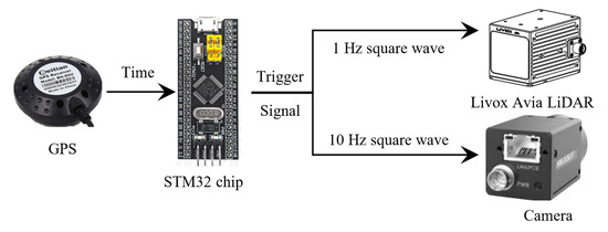
Figure 4.
Synchronized triggering of camera and LiDAR.
4. 3D Reconstruction Using LiDAR–Camera Fusion
4.1. Calibration and Matching of Laser Point Clouds to Images
The subsequent step involves calibrating the camera and LiDAR to establish 2D-3D correspondences, thereby achieving spatial synchronization between the two sensors. This process fundamentally relies on constructing matched point pairs between 2D images and 3D point clouds using a geometric calibration target to estimate the relative rotation and translation. The calibration of multi-sensor systems, such as cameras and LiDARs, constitutes the foundation for integrated measurement platforms. While this field has been extensively researched in recent years, most existing calibration methods target 360° rotating mechanical LiDARs. When applied to solid-state LiDARs or non-repetitive scanning LiDARs, challenges arise due to inhomogeneous point cloud density across scanning directions and inconsistent ranging error distributions. To address these challenges, specialized calibration methods for solid-state LiDARs have been proposed. For instance, the ACSC method [29] employs a spatiotemporal geometric feature extraction approach combined with intensity distribution analysis to estimate 3D corner points in point clouds. This technique enables precise corner detection under non-repetitive scanning conditions, even with uneven point density and reflectivity variations. Once corner points are detected in both point clouds and images, a system of equations is constructed to compute the extrinsic matrix.
The ACSC calibration method comprises three sequential phases: refined point cloud processing, corner detection, and extrinsic matrix estimation. The first phase involves denoising and enhancing point cloud features to mitigate inhomogeneity caused by non-repetitive scanning. Initially, temporal integration of the point cloud is performed. Compared to single-frame processing, continuous scanning over an extended duration generates denser point clouds for 3D objects, leveraging the inherent advantages of non-repetitive scanning. In this study, a checkerboard panel is selected as the calibration target. When visualizing the point cloud via intensity values, distinct patterns emerge between white and black checkerboard squares, analogous to image representations. However, the direct accumulation of raw point clouds introduces noise aggregation across frames, leading to blurred results. To counteract this, statistical outlier removal is applied to each input frame by analyzing neighborhood point density in the temporal domain. Post-integration, the surface normal distribution exhibits enhanced continuity compared to single-scan data. Subsequent segmentation based on normal vector differences and target similarity metrics enables cluster ranking, with the minimal-variation cluster retained for checkerboard localization. Furthermore, point cloud feature enhancement techniques are implemented to refine the checkerboard point cloud, ensuring noise-free and geometrically precise data. The specific procedure begins with detecting the boundary lines of the checkerboard panel. Subsequently, background point clouds outside these boundaries are filtered out, yielding a refined point cloud exclusively containing the checkerboard. An iterative optimization method is then applied to align with an idealized plane. The optimization process is formulated as follows:
where A, B, C, and D denote the estimated parameters of the fitted plane, and represents the standard deviation of distances from points in to the fitted plane. To address the inhomogeneous point cloud density, a voxel grid-based stochastic sampling method is applied to the refined point cloud . This sampling strategy ensures that the post-sampling point density does not exceed the maximum density observed in the original voxel grid, thereby homogenizing spatial distribution while preserving geometric fidelity.
After optimizing the point cloud, the next step is to detect the coordinates of corner points in the point cloud. The ACSC calibration method employs a nonlinear optimization approach to detect corner points. The core of this method lies in designing a similarity function to estimate the pose difference between the measured values P of checkerboard corners solved from reflectance and the mathematical model S of checkerboard corners. Based on this difference, the L-BFGS algorithm [30] is used to optimize the measured values of the corner points.
Once the corner coordinates are obtained, the Perspective-n-Point (PnP) algorithm can be directly applied to solve the extrinsic matrix. This study adopted the subpixel corner detection algorithm for extracting checkerboard corners from images. When using the algorithms mentioned above to calibrate the extrinsic parameters between the camera and LiDAR, the collected point cloud and final matching results are shown in Figure 5. In this section, the LiDAR and camera calibration toolbox in MATLAB (version 2022b) is used to calibrate the image and point cloud. After importing the calibrated image and the preprocessed point cloud, the program will compute the rotation and translation matrices for transforming the point cloud to the camera coordinates. After the calibration is completed, to verify the accuracy of the calibration, the point cloud is projected onto the image using the transformation matrix obtained from the calibration, and the translation error and reprojection error are obtained to be 2.61 mm and 2.48 pixels, respectively, as shown in Figure 5b.
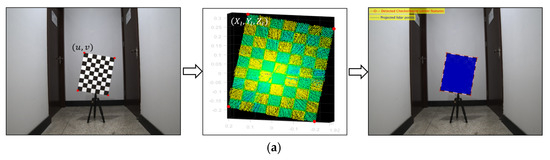
Figure 5.
Calibration of LiDAR and camera. (a) The collected image, point cloud, and results of point cloud to image projection and (b) translation error and reprojection error.
4.2. 3D Reconstruction Using Point Cloud and Image Fusion
Following the methodological framework in Figure 1, this section presents the adopted LiDAR–camera–IMU fused 3D mapping method. Multi-sensor fusion for 3D reconstruction and localization has been a key research focus in robotics in recent years. LiDAR, cameras, and IMUs are the most commonly used sensors, and SLAM methods employing these sensors individually or in combination have proliferated. Representative examples include visual odometries such as LSD-SLAM and DSO, visual-inertial odometries like ORB-SLAM3, and LiDAR-inertial odometries such as LOAM-SLAM and FAST-LIO [31,32,33]. While these methods have been extensively validated in laboratory tests and outdoor urban environments, real-world scenarios, particularly bridge surroundings, often suffer from sparse structural features and texture-deficient fields of view, posing new challenges to maintaining algorithmic robustness. Fully leveraging the complementary strengths of LiDAR, cameras, and IMUs is critical to ensuring mapping stability when single-sensor feature detection capabilities degrade. Recent advances in multi-sensor fused 3D mapping include R3LIVE++, R3LIVE, LVI-SAM, and FAST-LIVO [34,35,36].
Among these, R3LIVE++ is an enhanced algorithm derived from R3LIVE and R2LIVE. It consists of two independent subsystems: LIO and VIO modules. The LIO subsystem, directly adopting the FAST-LIO2 algorithm, leverages LiDAR and IMU measurements to establish the geometric structure of the global map. The VIO subsystem, a novel contribution of R3LIVE++, reconstructs the map’s texture using visual-inertial data. This VIO tracks camera poses by minimizing photometric discrepancies between sparse pixel sets in current images and precomputed radiation maps. Frame-to-map alignment mitigates odometric drift, while sparse pixel sampling constrains computational overhead. Additionally, the VIO estimates camera exposure time online to recover true environmental radiance.
Similarly, LVI-SAM integrates LIO and VIO subsystems. Its VIO initializes using LIO estimates and employs LiDAR measurements to extract depth information for visual features, thereby improving accuracy. Conversely, the LIO utilizes VIO-derived pose estimates as initial values for point cloud registration. This framework uses VIO to construct the global 3D map and perform loop closure detection, while LIO optimizes the results. The system maintains mapping continuity even if one subsystem fails, ensuring robustness in textureless or feature-scarce environments.
In contrast to the above vision–LiDAR fusion approaches, FAST-LIVO prioritizes computational efficiency, enabling real-time operation on low-performance Advanced RISC Machines (ARM) boards. Its LIO subsystem incrementally appends newly scanned raw points to a dynamically updated point cloud map. The VIO subsystem aligns new images by minimizing direct photometric errors using image patches associated with the point cloud map, bypassing explicit visual feature extraction. The workflow of this method is illustrated in Figure 6.
Figure 6.
Flow of the reconstruction methodology employed.
The state estimation method in FAST-LIVO employs a tightly coupled error-state iterative Kalman filter (ESIKF) to fuse LiDAR, camera, and IMU data. This method defines the IMU state at the first timestamp as the global coordinate system and estimates subsequent frame poses through a state transition model. The state and covariance matrix at the (i + 1)-th timestamp are derived via forward propagation. For the LiDAR measurement model in the frame-to-map update phase, the system first removes motion distortion from the input point cloud. During frame-to-map registration, newly observed points are assumed to lie on planes formed by their nearest neighbors in the map. To identify these planes, prior pose estimates project the points into the map, where the five closest points to each projected point are retrieved to fit a local plane.
For the visual measurement model, the method performs sparse direct frame-to-map image alignment in a coarse-to-fine manner by minimizing photometric errors. In map management, the LiDAR global map follows the incremental KD-tree approach from FAST-LIO2, providing interfaces for point querying, insertion, and deletion. The visual global map adopts an axis-aligned voxel-based data structure, where voxel hash tables enable the rapid identification of map points relevant to the current frame. After aligning a new image frame, image patches from the current frame are appended to map points within the field of view, ensuring uniform distribution of effective patches across viewing angles.
This workflow allows the VIO subsystem in FAST-LIVO to reuse LiDAR point clouds while bypassing visual feature extraction, triangulation, and optimization, significantly reducing computational demands. Consequently, the algorithm maintains robust performance in sensor-degraded environments with limited processing resources. Given FAST-LIVO’s superior runtime efficiency and mapping stability compared to other algorithms like R3LIVE++ and LVI-SAM, this study adopts FAST-LIVO as the LiDAR–camera fused 3D mapping framework.
4.3. Bridge Component Segmentation Using Image Segmentation and Point Cloud–Image Matching
After obtaining the 3D point cloud of the bridge through the aforementioned steps, the automated extraction of bridge geometry requires identifying key structural components from the large-scale point cloud, whose edge geometries collectively define the bridge’s linear form. The specific geometry of interest varies across bridge types and operational scenarios. For example, during the construction phase of suspension bridges, the cable geometry is a critical measurement target, necessitating the segmentation of main cable point clouds. In load-testing scenarios, the deck geometry becomes the focus, requiring the segmentation of girder point clouds. As this study focuses on a concrete arch bridge, the segmentation target in this section is the bridge arch. Once the arch is segmented from the images captured during UAV flights, the 2D mask of the arch in the images must be projected back into the 3D point cloud to extract the 3D coordinates of its geometry. This reconstruction leverages the pose information of each image, camera calibration parameters, and LiDAR–camera calibration results from prior steps. By reprojecting the arch mask into the 3D point cloud, the edge coordinates of the corresponding 3D points directly represent the bridge’s critical geometry. Unlike the existing algorithms based on point cloud processing, the proposed method is essentially a 2D image segmentation method that first segments the bridge’s components from the 2D image. Then it iterates through all the point clouds projected to the image plane according to the transform matrix calibrated from the image and the point cloud. Then the points projected in the masks of the components of the bridge are the point clouds of the segmented components. This method not only makes full use of the image and point cloud data contained in the system but also avoids the direct processing of large-scale point clouds, which reduces the algorithm’s requirements for computer arithmetic power. The algorithmic workflow for this section is illustrated in Figure 7.
Figure 7.
Procedure for the calculation method of bridge geometric shape.
As shown in Figure 7, the proposed method can be divided into two main steps: (1) Fine-grained segmentation of bridge components in images. (2) Three-dimensional coordinate resolution of these components. The core of the first step lies in addressing the identification and segmentation of bridge components using a high-precision segmentation network. Instance segmentation, a critical research direction in computer vision, aims to detect targets in input images and assign category labels to each pixel of the targets. Unlike conventional image segmentation tasks such as human body recognition or structural defect segmentation, where coarse mask edges are acceptable, most existing instance segmentation networks produce masks with rough boundaries, particularly in low-contrast scenarios where target and background differentiation are minimal. This limitation leads to degraded edge recognition accuracy.
In this study, the edge segmentation precision of bridge components directly affects the segmentation results of corresponding point clouds and consequently the accuracy of 3D coordinate resolution. Therefore, when applying instance segmentation networks, the focus is on improving the segmentation accuracy of component edges.
To address this challenge, we propose a transformer-based instance segmentation network designed to refine edge recognition and segmentation. The architecture of this network is illustrated in the accompanying figure. Building on the initial segmentation results from existing networks, our method employs a transformer structure for secondary prediction, specifically targeting edge regions [37]. For the critical edge areas of segmentation targets, a quadtree structure is constructed to represent discrete points across multiple hierarchical levels. A transformer-based segmentation network is utilized to predict instance labels for each tree node, given their distribution in discontinuous spatial domains. This network comprises three modules: a node encoder, a sequence encoder, and a pixel decoder. The node encoder enriches the feature representation of each point, the sequence encoder processes node sequences through a transformer-based architecture, and the pixel decoder predicts instance labels for each point. By serializing sparse feature points across scales and leveraging multi-head attention mechanisms, the model dynamically models multi-scale sparse features while enabling long-range comparisons and cross-hierarchy associations among feature points.
As illustrated in Figure 8, the network first constructs a quadtree comprising information loss nodes at different hierarchical levels. These nodes originate from a region of interest (RoI) pyramid but exhibit varying feature granularities due to their hierarchical differences. Information loss nodes from lower-level RoIs (28 × 28 resolution) correspond to four child nodes in their adjacent higher-level RoIs (56 × 56 resolution). To reduce computational complexity, pixels predicted as loss nodes are further decomposed into upper layers, with the maximum tree depth set to 3. The detection of information loss regions follows a bottom-up cascaded design. As shown on the right side of Figure 8, the lowest-level RoI features (28 × 28) and initial object mask predictions are first fed into a lightweight fully convolutional network (3 × 3 convolution) to predict quadtree root nodes. Each root node is decomposed into four child nodes in the adjacent higher-level RoI layer, extending from 28 × 28 to 56 × 56 resolutions. For higher-level RoI features, the mask from the preceding loss region detection is upsampled and concatenated with the current RoI features. A single 1 × 1 convolutional layer then predicts finer-grained information loss nodes, ensuring the detection module remains computationally efficient.
Figure 8.
Structure of the hierarchical bridge component extraction network.
Since the proposed method is applied to the geometry measurement of a concrete arch bridge in the testing phase, this section focuses on arch geometry measurement as a case study. A dataset of 300 UAV-captured images of bridge arches under varying illumination conditions was compiled. These images were manually annotated to create the training and evaluation dataset, as exemplified in Figure 9.
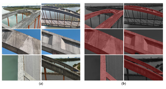
Figure 9.
The established bridge arch segmentation dataset. (a) Raw images captured by UAV and (b) manual labeling results.
The network was trained on hardware comprising an i7-11700K CPU from Intel Company, USA, 32 GB RAM, and an RTX 3090 GPU from NVIDIA Company, USA. The PyTorch (version 1.13.0) framework is used. Training parameters included 1000 iterations with a learning rate of 0.001. During training, the test accuracy of the predicted masks evolved as shown in Figure 10a, ultimately reaching 94.23% upon completion. The trained network was then applied to automatically segment arch regions in UAV-captured images of the bridge, with segmentation results demonstrated in Figure 10b. For a 4000 × 3000-pixel image, the automatic segmentation process required approximately 0.5 s.
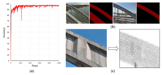
Figure 10.
Training results of the hierarchical bridge component segmentation network. (a) Accuracy during training, (b) segmentation results of the trained network, and (c) segmented point cloud after applying the image to point cloud matching.
Subsequently, following the workflow proposed in Figure 7, the fused LiDAR–camera system’s images and point clouds were processed. Segmentation results are illustrated in Figure 10c. For an input image and a LiDAR point cloud frame (with a 100 ms integration time), the total processing time from automatic arch segmentation in the image to point cloud segmentation averaged 2 s.
5. Field Test
The tested bridge is a concrete arch structure, as shown in Figure 11. With a main span of 140 m and a bridge width of 8 m, this structure was constructed in the 1970s. After decades of service, the bridge exhibits issues such as arch deformation and lateral tilting, necessitating precise 3D geometry inspection to assess its structural condition.
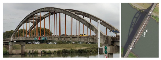
Figure 11.
Overview of the test bridge.
Three methods were employed to reconstruct the 3D model of the bridge during testing: (1) A high-precision TLS was used for multi-station scanning across the entire bridge. The scanning setup comprised 14 stations, with 40 retroreflective targets pre-installed on the bridge surfaces to facilitate accuracy validation. The TLS device (VZ-400i from RIEGL Company, Austria) offers a specified accuracy of 3 mm at 50 m, making its acquired geometry the reference ground truth. (2) A UAV-mounted mapping camera captured multi-view images of the bridge, which were processed using commercial 3D reconstruction software to generate a point cloud. (3) The proposed LiDAR–camera fused system performed rapid scanning while the UAV flew along predefined trajectories outside the bridge. The TLS field workflow and the resulting point cloud are shown in Figure 12. The weather for data collection was a clear day with sufficient light and a wind speed of category 3, and collection began at 12:00 noon to minimize shadows on the bridge surfaces and to avoid degradation of the image quality of the camera due to backlighting. The UAV photogrammetry method collected 2068 images, with the flight paths, operational procedures, and reconstructed point cloud detailed in Figure 13. The proposed system’s testing process and acquired point cloud are illustrated in Figure 14.
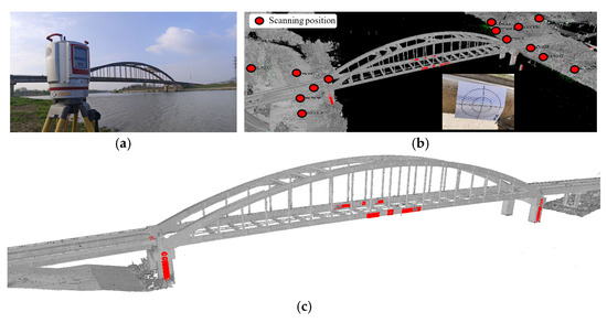
Figure 12.
Point clouds of the bridge reconstructed by high-precision TLS. (a) VZ-400i TLS, (b) scanning station layout and reflector settings, and (c) acquired 3D point cloud of the bridge.
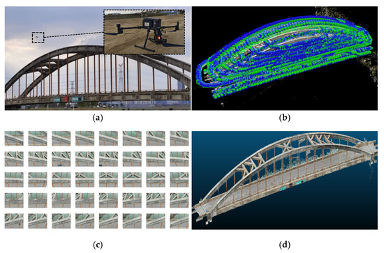
Figure 13.
Three-dimensional reconstruction results of the bridge using UAV oblique photogrammetry. (a) UAV flight photography process, (b) location of images acquired by the UAV, (c) images of the bridge arch, and (d) 3D reconstruction results of the bridge.
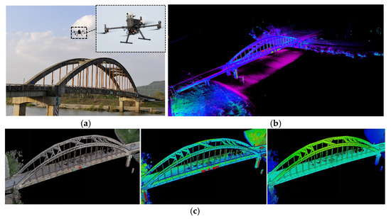
Figure 14.
Three-dimensional point cloud of the bridge reconstructed using the proposed method. (a) UAV flight scanning process, (b) reconstruction result displayed in real time during the flight, and (c) reconstructed 3D point cloud. Left: true color, middle: reflectivity assignment, right: height assignment.
For TLS scanning, the angular resolution was set to 0.02°, with each station requiring 3 min. During scanning of the bridge’s four sides, one station per side was selected for high-resolution scanning at 0.01° angular resolution, extending the scan time to 7 min per station. The scanner operated at a laser pulse repetition rate of 1200 kHz, achieving a maximum range of 250 m. Field scanning totaled approximately 2 h, followed by 2 h of data registration comprising manual coarse alignment and automated fine registration. The entire TLS-based workflow required 4 h, yielding an initial point cloud of 882 million points. Manual segmentation isolated the bridge structure, resulting in a refined point cloud of 193 million points.
For the UAV oblique photogrammetry-based 3D reconstruction method, data acquisition involved a combination of flight path planning software and manual localized photography to capture images of the bridge. The collected images included both long-range and close-range shots, with the latter achieving a pixel resolution of approximately 1.22 mm/pixel. The UAV platform used was a DJI M300 RTK equipped with a DJI P1 mapping camera. The UAV can provide 40 min of endurance per session, while the camera has a sensor measuring 35.9 mm × 24 mm with an effective pixel count of 45 megapixels and can capture images of 8192 × 5460 pixels. The camera automatically takes pictures at a rate of one per second while in flight. A close-range image of one arch is shown in Figure 13c, while Figure 13b illustrates the spatial distribution of images. The total image acquisition time was approximately 5 h, including an additional 3 h for preliminary data collection and the rough 3D model reconstruction required for flight path planning. After acquiring 2068 images, existing mature multi-view 3D reconstruction software was employed to generate the bridge point cloud. Considering computational efficiency, the open-source COLMAP software (version 3.12.0) was selected, which logged time costs for each processing stage: 0.2 h for feature detection, 11.67 h for feature matching, 21.45 h for sparse point cloud reconstruction, and 16.35 h for dense point cloud generation. The processing hardware comprised an Intel i7-11700K CPU, RTX 3090 GPU, and 64 GB RAM, resulting in a total processing time of 57.67 h. The final point cloud contained 255 million points, which was manually segmented to remove background noise, yielding a refined bridge point cloud of 167 million points.
The 3D scanning process using the proposed method is depicted in Figure 14a. During the test, the acquisition frequency of the LiDAR and the camera was 10 Hz, the frequency of the IMU was 200 Hz, the point cloud acquisition rate of the LiDAR was 240,000 points/second, and the size of the image acquired by the camera was 4000 × 3036 pixels. Since the LiDAR–camera fusion system operates continuously from UAV takeoff, unaffected by translational or rotational motions, the drone only needed to be on the bridge at an appropriate distance (15 m in this test) for at least one complete cycle. In this test, two flights were conducted, totaling 10 min from takeoff to landing. Real-time point cloud updates were displayed via wireless video transmission from the onboard computer, gradually revealing the bridge’s whole geometry as coverage expanded (Figure 14b). The reconstructed point cloud (Figure 14c) contained 18.7448 million raw points, reduced to 12.0692 million after manual background removal.
The three point cloud acquisition methods were compared in terms of accuracy and processing speed, and 80 retroreflective targets (40 per bridge side) were analyzed for accuracy validation. Coordinates extracted from TLS data served as ground truth, as shown in Figure 15a, while the proposed method directly identified targets via reflectivity, as shown in Figure 15b. UAV photogrammetry required manual target localization by averaging the corner coordinates of each target, as shown in Figure 15c.
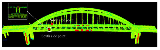
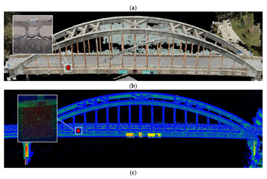
Figure 15.
Reflective targets observed in point clouds acquired by three methods. (a) Reflective targets observed by high-precision TLS, (b) reflective targets observed by UAV oblique photogrammetry, and (c) reflective targets observed by the proposed method.
Since the point clouds from the three methods resided in different coordinate systems, the relative coordinates of each target were calculated to analyze errors across methods. Using the first target as the reference point, the relative coordinates of other points were computed to align all measurements into a unified coordinate system. Figure 16 and Figure 17 illustrate the positional errors of UAV oblique photogrammetry and the proposed method relative to the high-precision laser scanning reference. The results reveal significantly larger errors in photogrammetry-derived target coordinates compared to the proposed method. Specifically, for X-axis measurements, the mean error of photogrammetry was 0.452 m, whereas the proposed method achieved 0.083 m, corresponding to 18.36% of photogrammetry’s error. For Y-axis measurements, photogrammetry exhibited a 0.602 m error against 0.103 m for the proposed method, representing 17.11% of the former. For Z-axis measurements, errors were 0.184 m for photogrammetry and 0.061 m for the proposed method, equivalent to 33.15%. Overall, the proposed method reduced the average error by 77.13% compared to oblique photogrammetry.
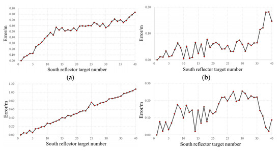
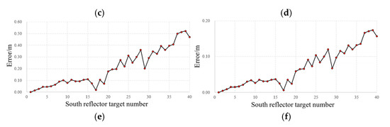
Figure 16.
Measurement errors of the three methods compared on the south side of the bridge. (a) x-coord errors in oblique photography, (b) x-coord errors in the proposed method, (c) y-coord errors in oblique photography, (d) y-coord errors in the proposed method, (e) z-coord errors in oblique photography, and (f) z-coord errors in the proposed method.
Figure 17.
Measurement errors of the three methods compared on the north side of the bridge. (a) x-coord errors in oblique photography, (b) x-coord errors in proposed method, (c) y-coord errors in oblique photography, (d) y-coord errors in proposed method, (e) z-coord errors in oblique photography, and (f) z-coord errors in proposed method.
The reconstruction efficiency of the three methods was further compared based on field and computational processing times, as summarized in Table 1. The total time for the proposed method amounted to merely 4.18% of the laser scanning workflow, while photogrammetry required 14.42 times longer than laser scanning. However, the proposed method generated fewer points due to the LiDAR module’s lower acquisition rate of 240,000 points per second compared to the laser scanner’s 1.2 million points per second, combined with significantly shorter scanning durations. Despite this, the point cloud density from the proposed method proved sufficient for geometry measurement. Notably, the laser scanner produced sparse point clouds at mid-span regions due to excessive scanning distances, whereas the proposed method maintained uniform density across all bridge sections through consistent proximity during scanning. Additionally, both laser scanning and photogrammetry demanded substantial computational memory and slower processing speeds, often requiring point cloud down-sampling for analysis on low-performance systems.

Table 1.
Comparison of the time consumption of the three methods in the reconstruction.
6. Conclusions
This study proposes a LiDAR–camera fused 3D reconstruction and automated component segmentation method for bridge geometry measurement. By synergizing the strengths of LiDAR point clouds and images, the proposed method achieves higher accuracy and efficiency in 3D reconstruction than image-based approaches. Unlike stationary high-precision laser scanning, it leverages image–point cloud correspondences for rapid segmentation, bypassing the direct processing of massive point clouds. Field tests on in-service bridge geometry inspection yield the following conclusions:
- (1)
- For LiDAR–camera data fusion, the method employs inertial navigation-based point cloud de-distortion, calibration target-based sensor alignment, and tightly coupled image–point cloud fusion to reconstruct large-scale 3D environments dynamically. The integrated system demonstrates rapid and stable 3D point cloud reconstruction for inspecting an in-service bridge.
- (2)
- An image-guided segmentation framework is proposed to address challenges in automated component segmentation from large-scale bridge point clouds. It maps 2D segmentation results to 3D point clouds, incorporating a coarse-to-fine segmentation network that achieves 94.23% accuracy in bridge component identification.
- (3)
- In the validation of an in-service bridge, it is demonstrated that the measurement accuracy of the proposed method is 83 mm in the X-axis direction, 103 mm in the Y-axis direction, and 61 mm in the Z-axis direction. The average error is reduced by 77.13% compared to the widely used method of UAV-based oblique photography. The total processing time is equivalent to 4.18% of the method using stationary laser scanning and 0.29% of the technique of UAV-based oblique photography.
When applying the proposed method to inspect the geometric shape of in-service bridges, there are limitations that need to be overcome and improved in future research. Firstly, the LiDAR in the constructed system is a low-cost, non-repeating scanning LiDAR, which is less accurate at the hardware level than the expensive, high-precision LiDAR. This resulted in an error of 8.3 cm in the reconstructed bridge compared to the static TLS scanner. The selection of higher accuracy LiDAR in the future is expected to improve the accuracy of the proposed method further. Secondly, the automated segmentation network of bridge components currently trained is only for the segmentation of arches of concrete arch bridges, so the proposed method can only realize the detection of the arch’s line shape at present. And because the proposed method for segmenting the point cloud of the components of a bridges is not to process the point cloud of the bridge directly but to segment the image first, and then to segment the point cloud projected in the mask of the components according to the calibration results of the image and the point cloud, the method can only be applied to the data collected by the proposed LiDAR–camera fusion system rather than the data collected by the other devices. In subsequent research, the datasets including bridge cables, box girder girders, and bridge towers will be added, so that the proposed method can be applied to more types of bridges and bridge components for geometric shape measurement.
Author Contributions
S.J.: Conceptualization, Methodology, Validation, Writing—original draft, Writing—review and editing, Funding Acquisition. Y.Y.: Methodology, Validation, Writing—original draft, Writing—review and editing. S.G.: Conceptualization, Validation. J.L.: Methodology, Validation. Y.H.: Conceptualization, Funding Acquisition. All authors have read and agreed to the published version of the manuscript.
Funding
The research presented was financially supported by the Key Laboratory of Target Cognition and Application Technology (No.: 2023-CXPT-LC-005), the Key Laboratory of Road and Railway Engineering Safety and Security (No.: STDTKF202303), and the Innovative training program for university students (No.: 202410304059Z).
Data Availability Statement
The data supporting this study’s findings are available from the corresponding author upon reasonable request.
Conflicts of Interest
The authors declare no conflicts of interest.
References
- Jiang, S.; Cheng, Y.; Zhang, J. Vision-guided unmanned aerial system for rapid multiple-type damage detection and localization. Struct. Health Monit. 2023, 22, 319–337. [Google Scholar] [CrossRef]
- Jiang, S.; Zhang, J.; Gao, C. Bridge Deformation Measurement Using Unmanned Aerial Dual Camera and Learning-Based Tracking Method. Struct. Control Health Monit. 2023, 2023, 4752072. [Google Scholar] [CrossRef]
- Tian, Y.; Zhang, C.; Jiang, S.; Zhang, J.; Duan, W. Noncontact cable force estimation with unmanned aerial vehicle and computer vision. Comput.-Aided Civ. Infrastruct. Eng. 2021, 36, 73–88. [Google Scholar] [CrossRef]
- Hu, F.; Zhao, J.; Huang, Y.; Li, H. Structure-aware 3D reconstruction for cable-stayed bridges: A learning-based method. Comput.-Aided Civ. Infrastruct. Eng. 2021, 36, 89–108. [Google Scholar] [CrossRef]
- Tian, X.; Liu, R.; Wang, Z.; Ma, J. High-quality 3D reconstruction based on fusion of polarization imaging and binocular stereo vision. Inf. Fusion 2022, 77, 19–28. [Google Scholar] [CrossRef]
- Zhang, S. High-speed 3D shape measurement with structured light methods: A review. Opt. Lasers Eng. 2018, 106, 119–131. [Google Scholar] [CrossRef]
- Hosamo, H.H.; Hosamo, M.H. Digital twin technology for bridge maintenance using 3d laser scanning: A review. Adv. Civ. Eng. 2022, 2022, 2194949. [Google Scholar] [CrossRef]
- Ma, Z.; Choi, J.; Sohn, H. Continuous bridge displacement estimation using millimeter-wave radar, strain gauge and accelerometer. Mech. Syst. Signal Process. 2023, 197, 110408. [Google Scholar] [CrossRef]
- Wang, F.; Zou, Y.; del Rey Castillo, E.; Ding, Y.; Xu, Z.; Zhao, H.; Lim, J.B. Automated UAV path-planning for high-quality photogrammetric 3D bridge reconstruction. Struct. Infrastruct. Eng. 2024, 20, 1595–1614. [Google Scholar] [CrossRef]
- Chen, S.; Laefer, D.F.; Mangina, E.; Zolanvari, S.M.I.; Byrne, J. UAV bridge inspection through evaluated 3D reconstructions. J. Bridge Eng. 2019, 24, 05019001. [Google Scholar] [CrossRef]
- Verykokou, S.; Ioannidis, C. An overview on image-based and scanner-based 3D modeling technologies. Sensors 2023, 23, 596. [Google Scholar] [CrossRef] [PubMed]
- Lin, Y.C.; Liu, J.; Cheng, Y.T.; Hasheminasab, S.M.; Wells, T.; Bullock, D.; Habib, A. Processing strategy and comparative performance of different mobile lidar system grades for bridge monitoring: A case study. Sensors 2021, 21, 7550. [Google Scholar] [CrossRef] [PubMed]
- Lu, R.; Brilakis, I. Recursive segmentation for as-is bridge information modelling. In Proceedings of the LC3 2017—Joint Conference on Computing in Construction (JC3), Heraklion, Greece, 4–7 July 2017; Volume I, pp. 209–217. [Google Scholar] [CrossRef]
- Mohammadi, M.; Rashidi, M.; Yu, Y.; Samali, B. Integration of TLS-derived Bridge Information Modeling (BrIM) with a Decision Support System (DSS) for digital twinning and asset management of bridge infrastructures. Comput. Ind. 2023, 147, 103881. [Google Scholar] [CrossRef]
- Shao, J.; Zhang, W.; Mellado, N.; Grussenmeyer, P.; Li, R.; Chen, Y.; Wan, P.; Zhang, X.; Cai, S. Automated markerless registration of point clouds from TLS and structured light scanner for heritage documentation. J. Cult. Herit. 2019, 35, 16–24. [Google Scholar] [CrossRef]
- Sun, L. Practical, fast and robust point cloud registration for scene stitching and object localization. IEEE Access 2022, 10, 3962–3978. [Google Scholar] [CrossRef]
- Tarabini, M.; Giberti, H.; Giancola, S.; Sgrenzaroli, M.; Sala, R.; Cheli, F. A moving 3D laser scanner for automated underbridge inspection. Machines 2017, 5, 32. [Google Scholar] [CrossRef]
- Feroz, S.; Abu Dabous, S. UAV-based remote sensing applications for bridge condition assessment. Remote Sens. 2021, 13, 1809. [Google Scholar] [CrossRef]
- Wang, D.; Gao, L.; Zheng, J.; Xi, J.; Zhong, J. Automated recognition and rebar dimensional assessment of prefabricated bridge components from low-cost 3D laser scanner. Measurement 2025, 242, 115765. [Google Scholar] [CrossRef]
- Zhu, Y.; Brigham, J.C.; Fascetti, A. LiDAR-RGB Data Fusion for Four-Dimensional UAV-Based Monitoring of Reinforced Concrete Bridge Construction: Case Study of the Fern Hollow Bridge Reconstruction. J. Constr. Eng. Manag. 2025, 151, 05024016. [Google Scholar] [CrossRef]
- Li, J.; Peng, Y.; Tang, Z.; Li, Z. Three-dimensional reconstruction of railway bridges based on unmanned aerial vehicle–terrestrial laser scanner point cloud fusion. Buildings 2023, 13, 2841. [Google Scholar] [CrossRef]
- Huang, Y.; Du, Y.; Shi, W. Fast and accurate power line corridor survey using spatial line clustering of point cloud. Remote Sens. 2021, 13, 1571. [Google Scholar] [CrossRef]
- Xu, Y.; Zhang, J. UAV-based bridge geometric shape measurement using automatic bridge component detection and distributed multi-view reconstruction. Autom. Constr. 2022, 140, 104376. [Google Scholar] [CrossRef]
- Kim, H.; Narazaki, Y.; Spencer, B.F., Jr. Automated bridge component recognition using close-range images from unmanned aerial vehicles. Eng. Struct. 2023, 274, 115184. [Google Scholar] [CrossRef]
- Xia, T.; Yang, J.; Chen, L. Automated semantic segmentation of bridge point cloud based on local descriptor and machine learning. Autom. Constr. 2022, 133, 103992. [Google Scholar] [CrossRef]
- Yang, X.; del Rey Castillo, E.; Zou, Y.; Wotherspoon, L.; Tan, Y. Automated semantic segmentation of bridge components from large-scale point clouds using a weighted superpoint graph. Autom. Constr. 2022, 142, 104519. [Google Scholar] [CrossRef]
- Jing, Y.; Sheil, B.; Acikgoz, S. Segmentation of large-scale masonry arch bridge point clouds with a synthetic simulator and the BridgeNet neural network. Autom. Constr. 2022, 142, 104459. [Google Scholar] [CrossRef]
- Yang, W.; Gong, Z.; Huang, B.; Hong, X. Lidar with velocity: Correcting moving objects point cloud distortion from oscillating scanning lidars by fusion with camera. IEEE Robot. Autom. Lett. 2022, 7, 8241–8248. [Google Scholar] [CrossRef]
- Cui, J.; Niu, J.; Ouyang, Z.; He, Y.; Liu, D. ACSC: Automatic calibration for non-repetitive scanning solid-state LiDAR and camera systems. arXiv 2020, arXiv:2011.08516. [Google Scholar] [CrossRef]
- Mannel, F.; Aggrawal, H.O.; Modersitzki, J. A structured L-BFGS method and its application to inverse problems. Inverse Probl. 2024, 40, 045022. [Google Scholar] [CrossRef]
- Campos, C.; Elvira, R.; Rodriguez, J.J.G.; Montiel, J.M.M.; Tardos, J.D. ORB-SLAM3: An accurate open-source library for visual, visual–inertial, and multimap slam. IEEE Trans. Robot. 2021, 37, 1874–1890. [Google Scholar] [CrossRef]
- Yi, S.; Lyu, Y.; Hua, L.; Pan, Q.; Zhao, C. Light-LOAM: A lightweight lidar odometry and mapping based on graph-matching. IEEE Robot. Autom. Lett. 2024, 9, 3219–3226. [Google Scholar] [CrossRef]
- Wu, F.; Beltrame, G. Direct sparse odometry with planes. IEEE Robot. Autom. Lett. 2021, 7, 557–564. [Google Scholar] [CrossRef]
- Lin, J.; Zhang, F. R3LIVE++: A Robust, Real-time, Radiance Reconstruction Package with a Tightly-coupled LiDAR-Inertial-Visual State Estimator. IEEE Trans. Pattern Anal. Mach. Intell. 2024, 46, 11168–11185. [Google Scholar] [CrossRef] [PubMed]
- Han, L.; Shi, Z.; Wang, H. A localization and mapping algorithm based on improved LVI-SAM for vehicles in field environments. Sensors 2023, 23, 3744. [Google Scholar] [CrossRef]
- Zheng, C.; Xu, W.; Zou, Z.; Hua, T.; Yuan, C.; He, D.; Zhou, B.; Liu, Z.; Lin, J.; Zhu, F.; et al. FAST-LIVO2: Fast, direct lidar-inertial-visual odometry. IEEE Trans. Robot. 2024, 41, 326–346. [Google Scholar] [CrossRef]
- Wang, J.; Yu, X.; Gao, Y. Feature fusion vision transformer for fine-grained visual categorization. arXiv 2021, arXiv:2107.02341. [Google Scholar] [CrossRef]
Disclaimer/Publisher’s Note: The statements, opinions and data contained in all publications are solely those of the individual author(s) and contributor(s) and not of MDPI and/or the editor(s). MDPI and/or the editor(s) disclaim responsibility for any injury to people or property resulting from any ideas, methods, instructions or products referred to in the content. |
© 2025 by the authors. Licensee MDPI, Basel, Switzerland. This article is an open access article distributed under the terms and conditions of the Creative Commons Attribution (CC BY) license (https://creativecommons.org/licenses/by/4.0/).