Performance Analysis of Model-Based Control for Thermoelectric Window Frames

Abstract

The Thermoelectric Window Frame (TEWF) can be adjusted by regulating the operating current to achieve the desired indoor temperature. However, indoor and outdoor ambient disturbances are inevitable, causing indoor temperature fluctuations and preventing them from reaching the set point. To solve the problem, a model-based control method is proposed to maintain the indoor temperature at the set point in this work. This method relies on a computational model for determining the operating current and a transient model for tracking variations in indoor temperature. Experimental results under various working conditions validate the two models. Moreover, indoor interference (e.g., changes in set point or air leaks due to occupants’ behavior) and outdoor interference (e.g., changes in the outdoor temperature) are incorporated into stable-state experiments. When these interferences occur, new operating currents are calculated for the new working conditions and applied to the TEWF. The results show that the indoor temperature significantly deviates from the desired values if the operating currents are not adjusted when disturbances occur. However, the indoor temperature can reach the set point by regulating the new operating currents in time, even during disturbances.

1. Introduction

The Peltier effect [1] allows thermoelectric (TE) systems to pump heat from one side to another when powered by electric currents. Due to their thermal characteristics, TE systems have been applied for temperature control across various domains [2]. In buildings, TE systems have been integrated into structural elements such as walls [3,4,5], windows [6,7], and ceilings [8,9] and incorporated into Heating, Ventilation, and Air-conditioning (HVAC) systems to enhance efficiency [10].

In practical building applications, although TE systems typically exhibit a lower coefficient of performance (COP) than HVAC systems [11], they can integrate well with solar systems, utilizing direct current to reduce grid power consumption and improve overall energy efficiency [12,13,14]. Additional benefits include their simple design, lightweight structure, reliability, and flexible applications [15]. Advances in high-performance thermoelectric materials [16], improved system construction for heat transfer [17,18], and optimization-driven control systems [19,20] can further enhance their thermal performance.

Effective control systems for TE systems are essential in building applications that require accuracy, responsiveness, robustness, and energy efficiency. These systems mitigate temperature disturbances and help to maintain a stable set point under variable conditions [21]. However, challenges arise due to the nonlinear dynamics and time-varying disturbances inherent in TE systems. To overcome this, some control methods have been developed or applied in existing studies on TE systems in buildings.

Proportional, Integral, Differential (PID) control, widely used for its simplicity and effectiveness, minimizes deviations between actual and target values by adjusting inputs based on tuned gain parameters [22]. However, it lacks the sophistication needed for more complex systems. In buildings, due to air temperature fluctuation, the initial tuned PID control unit may lead to users’ discomfort [23]. Li et al. [24] indicated that adaptive PID control offers improved performance with reduced overshoot, faster response, and more substantial anti-interference capability in an air-conditioning system. Nevertheless, improper tuning can lead to instability, and it remains limited in nonlinear or delayed systems.

Under dynamic conditions, Isik et al. [25] highlighted the reliability of fuzzy logic control, which recovers quickly from disturbances without requiring mathematical models. However, implementing fuzzy control requires careful consideration of the initial membership functions and fuzzy rules to address system dynamics and uncertainties [26]. Effective rule generation for TE systems is challenging, and enhancing accuracy often demands numerous membership functions, significantly increasing rule complexity.

Additionally, regarding model-free control, except for fuzzy logic control mentioned above, deep reinforcement learning control [27,28] also has the potential to deal with nonlinear, complex systems. Luo et al. [29] used TE coolers (TEC) to achieve the global optimal temperature for advanced electronic systems by controlling individual Peltier cells. They used a machine learning model to iterate all possible TEC assignments for attaining the global optimal solution. Therefore, model-free control does not need accurate mathematical models and can find the optimal solution after sufficient exploration. However, it requires a large amount of training data and high training costs and may incur high trial-and-error costs when applied to physical systems.

To address the limitations of the previously mentioned control methods, this study focuses on model-based control, which uses a system model for predictive control rather than corrective actions. Establishing an accurate model of TE systems enables prediction to reduce the need for real-world interactions and makes effective decisions even with limited data. This approach facilitates disturbance rejection and accounts for time-varying dynamics, such as indoor or outdoor temperature changes.

Kishore et al. [30] proposed model-based control to control the temperature of TE elements for rescue robots. Their method offers sufficient cooling performance along with optimum energy consumption. Wang et al. [31] introduced model-based control for the thermoelectric cooling based thermal management system of electric vehicles, and aimed at ensuring that the battery temperature remains within a safe range while minimizing energy consumption. Petryna et al. [32] implemented model-based control to optimize the operation of the TE heat pump and aimed to find the minimum of the cost function. Unlike the studies [30,31,32] mentioned above that primarily optimize energy consumption using model-based control, our approach focuses on improving temperature regulation accuracy while maintaining efficiency. Additionally, unlike the studies [30,31] that validate model-based control performance in simulations, this study implements and tests our approach in a real-world experimental setup, demonstrating its feasibility. Furthermore, our method accounts for real-world disturbances such as air leakage and outdoor temperature variation, making it more robust in practical applications.

Experimental assessments of model-based control for TE systems in buildings are still lacking. Therefore, in this work, one goal is to establish both computational and transient models for the Thermoelectric Window Frame (TEWF) with integral heat sinks based on our previous works [20,33] and validate the results against experimental data. The computational model can calculate the operating current under specific working conditions, while the transient model can simulate the timewise temperature change in interior space based on the corresponding current. Another objective is to propose the model-based control methodology that includes both models and verify its disturbance-rejection performance through experiments, considering the occupants’ disturbances and the time-varying dynamics in outdoor temperature.

The structure of this work is as follows: Section 2 describes the TEWF system, its electrical connection, and the experimental setup. Section 3 details the formulation of the computational and transient models of the TEWF and the proposed model-based control methodology. Section 4 validates the models with the experimental results and evaluates the control performance under interferences.

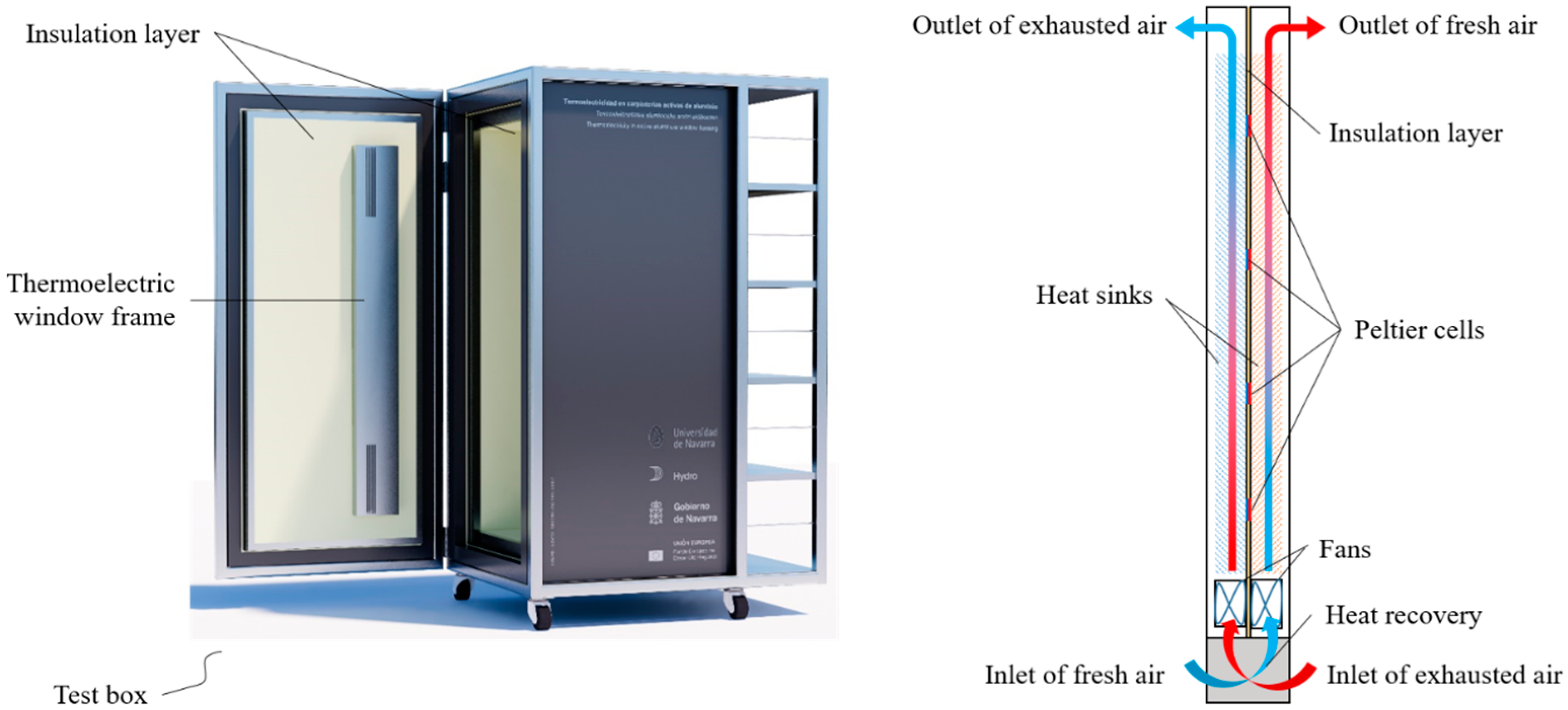
2. System Description

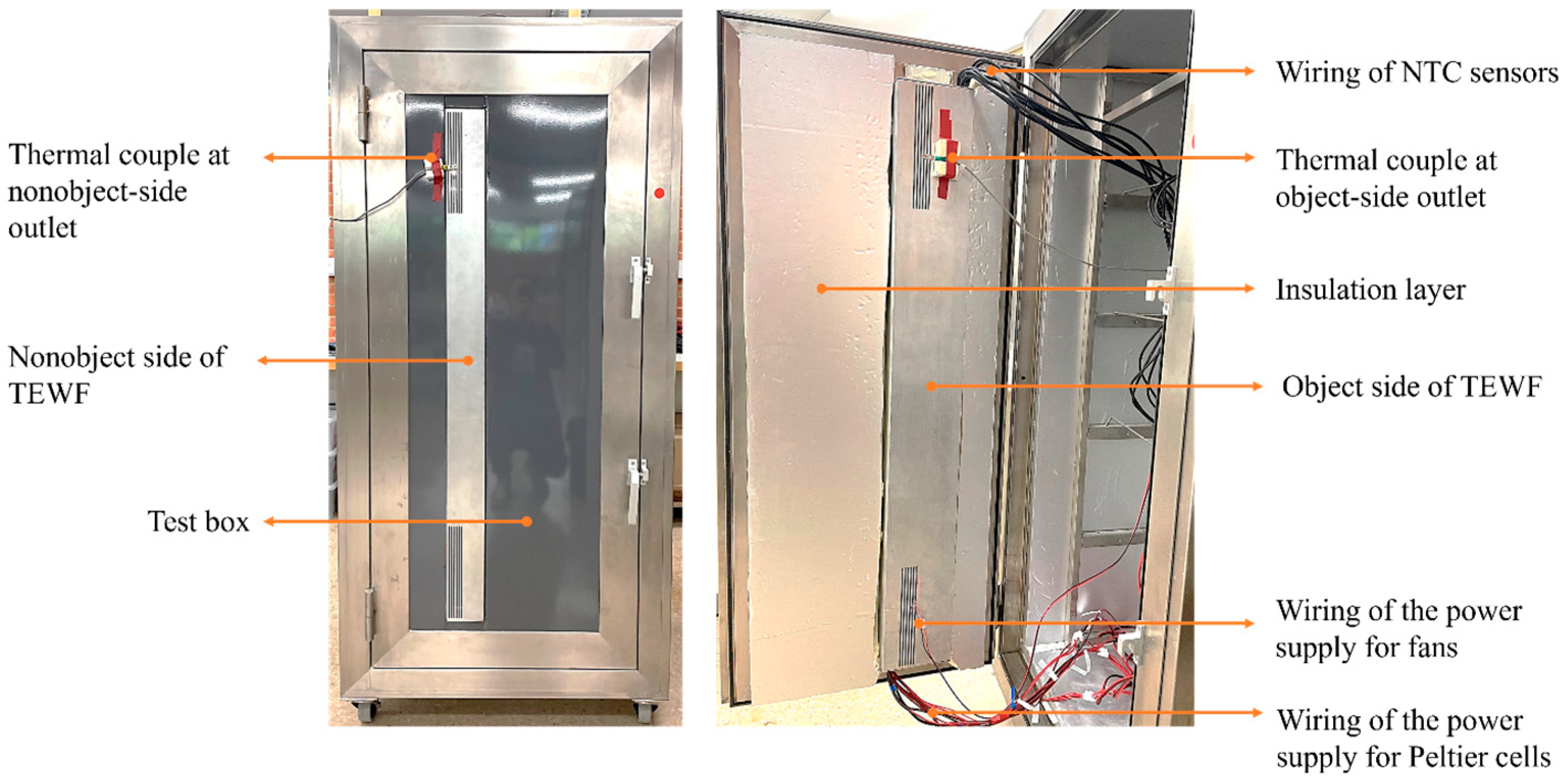
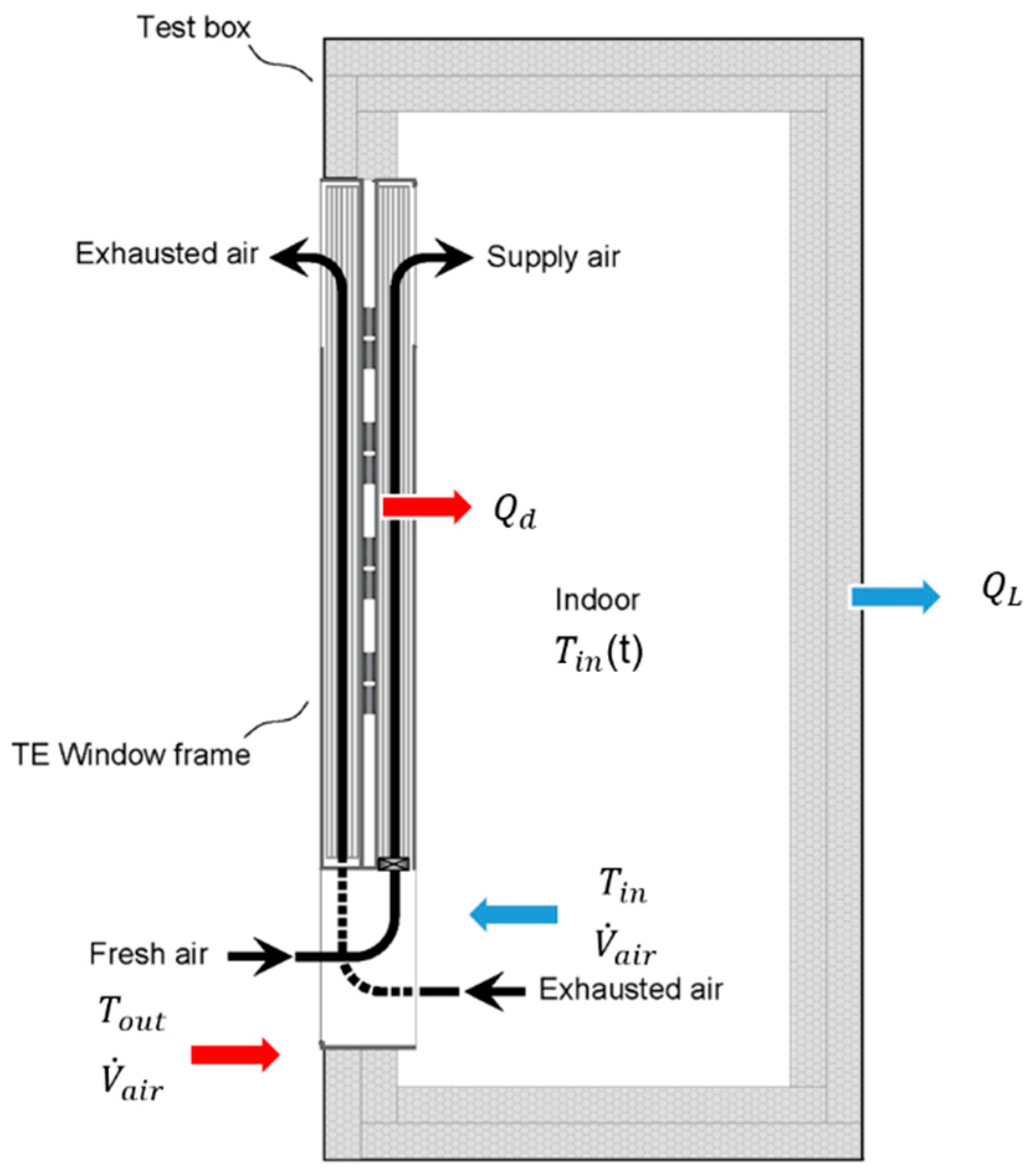
2.1. Experimental System

The experiment bench was built in previous work, and its constructive integration was presented [34]. Generally, as shown in Figure 1, Peltier cells and heat sinks are integrated as TE modules and then covered in shells as the TEWF. This TEWF is mounted within an insulated booth, measuring 720 mm in length, 795 mm in width, and 1520 mm in height. The experimental bench is built to assess the heating and cooling performance of the TEWF for indoor spaces or localized air-conditioning applications.

In this work, the TEWF consists of eight Peltier cells, two fans, and two heat sinks covered with aluminum shells, measuring 1200 mm in length, 90 mm in width, and 60 mm in height. As shown in Figure 1, airflows pass over the heat sinks, and the fans and power supply enable the process. Due to the Peltier effect [1], the cold, fresh airflow is warmed to the desired temperature in heating mode. Simultaneously, the wasted heat in the warm, exhausted airflow is pumped to the hot side from the cold side. In the cooling mode, reversing the current direction switches the roles of the cold and hot sides. The indoor temperature is controlled by adjusting the operating currents or the number of active Peltier cells, modulating the thermal capacity of the TEWF under a specific working condition.

Regarding the electric connection, as shown in Figure 2, power supplies for Peltier cells and fans and the data logs for Negative Temperature Coefficient (NTC) sensors and thermal couples are wired through the booth’s interior space. These components are controlled by a power distribution box and hosts located behind the booth. Detailed design information on the chambers and sensor cable routing has been previously presented [20].

Exactly as shown in Figure 3, the electric control system comprises power supplies, TEC microcontrollers [35], the monitoring host, the data log, and the sensors. The microcontrollers regulate the operating currents of Peltier cells and monitor their surface temperatures using NTC sensors. The host records data from the microcontrollers and the HOBO data log [36] for airflow and indoor and outdoor temperatures. Additionally, the operating current of the fans is adjusted by power supply 2 to regulate airflow rates. The specifications of the experimental equipment used are listed in

Table 1. Specifications of used experimental equipment.

Equipment	Type	Range	Accuracy
Temperature sensor	Film NTC thermistor	−30 °C to 120 °C	±1%
Temperature sensor	TMCx-HE U12	−40 °C to 50 °C	±0.25 °C
Power supply	PSI5040-10A	0 A to 10 A	≤0.2%
Data logger	HOBO U12-006	0 to 10 V	±2.5% ± 2 mV
Hot-wire anemometry	Testo 405i	0 to 30 m/s	±3% ± 0.1 m/s
Microcontroller	TEC-1122	−40 °C to 90 °C	<0.01 °C
		0 A to ±10 A	<1%

.

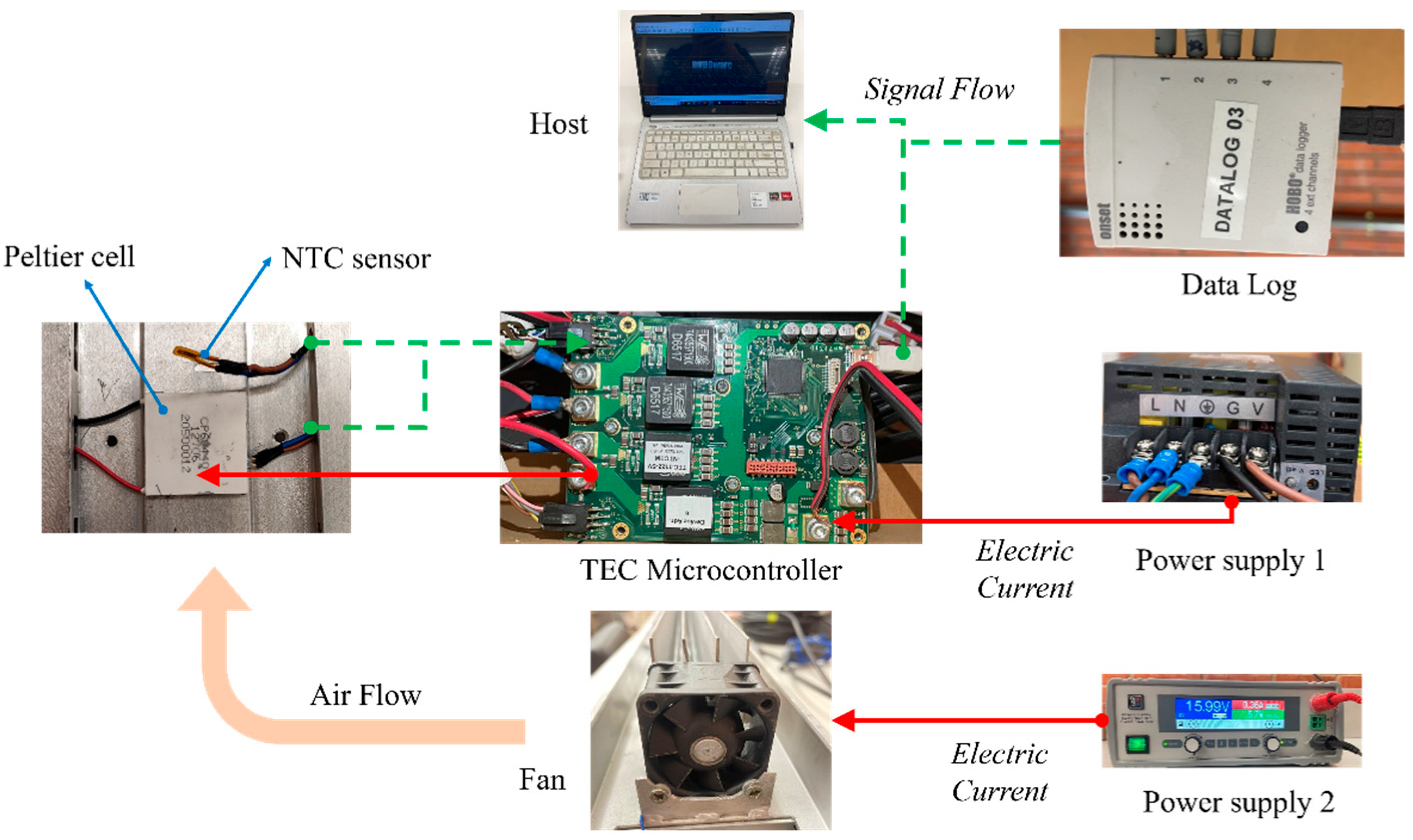
2.2. Experimental Setup

As illustrated in Figure 4, the electric control system can adjust the power strength of Peltier cells, the number of activated Peltier cells, and the airflow rates. Specifically, the power strength of Peltier cells can be regulated by two TEC microcontrollers according to the demand of the thermal capacity. Each TEC microcontroller controls four Peltier cells. The eight Peltier cells are connected in parallel, and the number of activated Peltier cells can be adjusted from four to eight by switching on or off some Peltier cells. Airflow rates can be controlled by changing the fan’s operating voltage.

In experiments, tests are conducted in laboratory ambient (20 ± 0.5 °C) and outdoor ambient (14 ± 0.5 °C). The TEWF operates to maintain an indoor set point of 22 °C to 28 °C in the laboratory ambience and 22 °C in the outdoor ambience with eight Peltier cells. The computational model works out their operating currents under specific working conditions and varies from 0 to 2.5 A to prevent extreme temperature differences between the hot and cold sides. The operating voltage of the fans can range from 12 V to 24 V. The variations in the indoor temperature are monitored over time and compared with the results of the transient model. Additionally, the interference of occupants’ behavior and the fluctuation of outdoor temperature are considered in experiments to test the performance against disturbances.

3. System Modeling

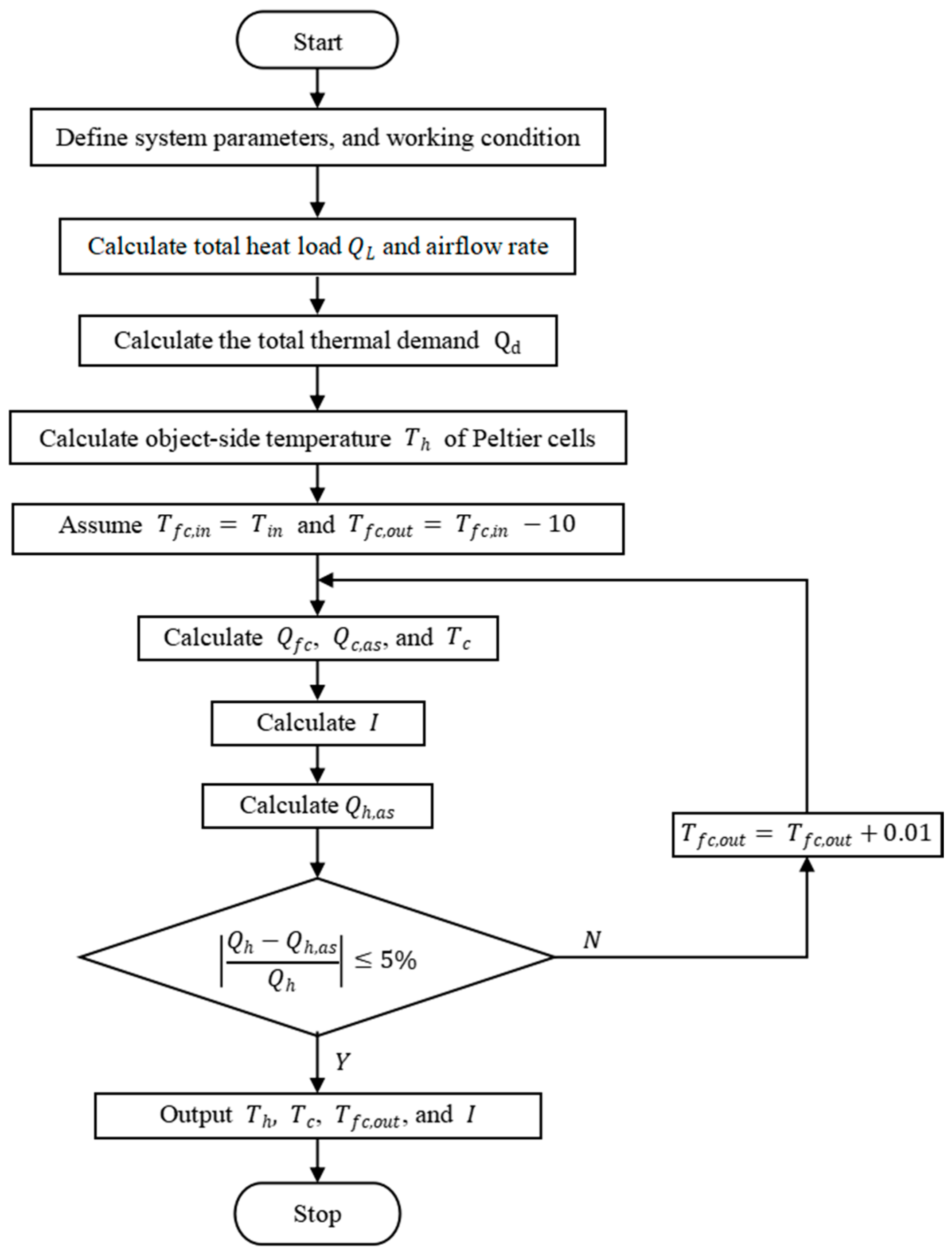
3.1. Computational Model

As depicted in Figure 5, with the variations in the heat load, the working conditions of the TEWF vary, resulting in fluctuations in the interior temperature. To maintain the set point, control systems facilitate the adjustment of the operating currents of the Peltier cells and the fans. This leads to changes in the surface temperatures of the Peltier cells and the airflow rate, which adjusts the thermal capacity of the TEWF and then adapts the interferences from the ambient. The real-time interior temperatures are compared to the set point. The controllers are utilized to output the control quantity of the operating currents based on the deviations between the real-time temperature and the set point.

Here, a steady-state model for the TEWF is established here to calculate the operating current under specific working conditions. When the working conditions change, the computational model determines a new operating current for the indoor set point. The model was used to analyze the impact of the number of activated Peltier cells on thermal performance. The operating current required for each Peltier cell to achieve a specific thermal capacity could be calculated iteratively, one TE module at a time. However, our experimental system utilized integral heat sinks. Hence, this study evaluates TEWF with integral heat sinks, and its computational model is outlined as follows, iterating the whole system at a time.

As illustrated in Figure 6, the system parameters and working conditions are first defined. Subsequently, the heat load Q_L can be worked out with the box surface area of 5.75 m² and the heat conductivity of 1.48 W/(K·m²), followed by determining the required airflow rate using the specified supply air temperature T_fh,out, as expressed in Equations (1) and (2) [37].

$$Q_L=K{A}_{box}(T_{in}-T_{out})$$

(1)

$${\dot{V}}_{air}={\displaystyle \frac{Q_L}{{\rho }_{air}{c}_p\left(T_{fh,out}-T_{in}\right)}}$$

(2)

Next, the total thermal demand, Q_d, including the exhausted heat, is determined using Equation (3) [37]. Then, the object-side surface temperature, T_h, of each Peltier cell can be calculated based on the relationship between the thermal demand, Q_d, and the temperature difference between the surface temperature and the average airflow temperature T_fh,m, as shown in Equation (4).

$$Q_d={\rho }_{air}{c}_p{\dot{V}}_{air}\left(T_{fh,out}-T_{out}\right)$$

(3)

$$T_h=Q_d{U}_h+T_{fh,m}=Q_d{U}_h+\left(T_{out}+T_{fh,out}\right)/2$$

(4)

When the total thermal demand, Q_d, is distributed across N Peltier cells, the thermal capacity required for each Peltier cell, Q_fh, is obtained. Then, the airflow passing the object side is heated up by the heat pumped from Peltier cells, Q_h. Considering heat loss, a heat transfer coefficient, ${\mathsf{\eta }}_h$, is introduced to account for the fraction of the heat Q_h transferred into the airflow [20], as described in Equation (5) [6].

$$Q_d=N{Q}_{fh}={\eta }_{h}N{Q}_h={\eta }_{h}N\left(\alpha I{T}_h+{\displaystyle \frac{1}{2}}{I}^2{R}_e-k\left[T_h-T_c\right]\right)$$

(5)

Finally, the desired current, I, can be determined by iteratively adjusting the surface temperature at the non-object side, T_c. As shown in Figure 6, it is assumed that the temperature, T_fc,in, of the incoming airflow at the cold side equals the indoor temperature, T_in, and decreases by 10 °C. Based on the assumption, the heat absorbed from the airflow, Q_fc, and the cold-side temperature, T_c, can be calculated as shown in Equations (6) and (7) [37]. Considering the heat transfer coefficient, η_c, at cold side, the cooling capacity, Q_c,as, can be gained based on Equation (8).

$$Q_{fc}=c_p{m}_{air}\left(T_{fc,in}-T_{fc,out}\right)/N$$

(6)

$$T_c=T_{fc,m}-Q_{fc}{U}_c=\left(T_{fc,in}+T_{fc,out}\right)/2-Q_{fc}{U}_c$$

(7)

$$Q_{c,as}={\displaystyle \raisebox{1ex}{$Q_{fc}$}\!\left/ \!\raisebox{-1ex}{${\eta }_c$}\right.}$$

(8)

From these calculations, the operating current, I, under the given assumption can be computed based on Equation (9) [6], with the property parameters Seebeck coefficient, α, of 0.05 V/K, electric resistance, Re, of 2.44 Ω, and heat transfer coefficient, k, of 0.57 W/K [20]. Since the Peltier cells of TEC-12706 used in the experimental system have a maximum electric current of 6.4 A, the operating current should satisfy the condition described in Equation (10).

$${\displaystyle \frac{1}{2}}{R_{e}I}^2-\alpha I{T}_{c}I+k\left[T_h-T_c\right]+Q_{c,as}=0$$

(9)

$$I={\displaystyle \frac{\alpha T_c-\sqrt{{\left[\alpha T_c\right]}^2-2R_e\left\{k\left[T_h-T_c\right]+Q_{c,as}\right\}}}{R_e}}$$

(10)

Once the operating current, I, is worked out, the heating capacity, Q_h,as, under the assumptions, can also be calculated, as shown in Equation (11). Simultaneously, the required heating capacity, Q_h, can be determined, as shown in Equation (5). Furthermore, the deviation between Q_h and Q_h,as can be analyzed. If the deviation exceeds 5%, the assumed temperature, T_fc,out, of the outgoing airflow at the cold side will be incremented by 0.01 °C in each iteration calculation until the deviation is within 5%. As a result, the temperature of the outgoing airflow at the cold side, the surface temperature of Peltier cells, and the operating current, I, can be yielded under the new working conditions.

$$Q_{h,as}=\alpha I{T}_h+{\displaystyle \frac{1}{2}}{I}^2{R}_e-k\left[T_h-T_c\right]$$

(11)

The steady-state model is used to calculate the desired operating current corresponding to the required thermal capacity under specific working conditions. Then, the operating current can be applied in the subsequent transient model to simulate the time-dependent indoor temperature profile. Additionally, when a system in stable operation is suddenly interfered with by the oscillations resulting from the outdoor ambient or occupants’ behavior, the heat load and indoor temperature fluctuate. In response, the TEWF should adjust to deliver a new thermal capacity for recovering a stable indoor ambient. During this process, the indoor temperature fluctuates but eventually returns to the set point under the new working conditions.

3.2. Transient Model

A transient model for the indoor temperature profile is established to simulate variations in indoor temperature under certain working conditions. As shown in Figure 7, regarding the heat transfer, the fresh airflow is air-conditioned by Peltier cells. The airflow at the object side provides the required thermal demand, Q_d, which is divided into two parts: one part addresses the heat load, Q_L, while the other is carried away by the exhausted airflow at the non-object side. Additionally, due to the possible disturbances from the occupants’ behaviors, an additional thermal capacity, Q_ad, is included. In the process, the indoor temperature fluctuates and generally adjusts to reach the set point. This process is mathematically described as shown in Equation (12).

$${\rho }_{in}{c}_p{V}_{box}{\displaystyle \frac{d{T}_{in}\left(t\right)}{dt}}=Q_d\left(t\right)+{\rho }_{fh}{c}_p{\dot{V}}_{fh}\left(t\right)T_{out}\left(t\right)-{\rho }_{fc}{c}_p{\dot{V}}_{fc}\left(t\right)T_{in}\left(t\right)-Q_L\left(t\right)-Q_{ad}\left(t\right)$$

(12)

To simplify the model, several assumptions are made. Firstly, the airflow is treated as an incompressible fluid, and phase transitions do not occur during the air-conditioning process. The specific heat capacity of air at constant pressure is taken as 1005 J/(kg·K). Consequently, the influence of air temperature on air density is negligible, allowing air density to be considered constant at 1.29 kg/m³. Next, under a given working condition, outdoor temperature fluctuations are minimal. Therefore, their effects on the heat load and thermal demand can be ignored under the given working condition. Parameters such as operating current, heat load, heat demand, airflow rate, and surface temperatures of Peltier cells are assumed constant under the given working condition. Consequently, the descriptive formula is simplified and expressed in Equations (13) and (14).

$${\rho }_{air}{c}_p{V}_{box}{\displaystyle \frac{d{T}_{in}\left(t\right)}{dt}}+{\rho }_{air}{c}_p{\dot{V}}_{air}{T}_{in}\left(t\right)+K(T_{in}\left(t\right)-T_{out})+\left(Q_{ad}-{\rho }_{air}{c}_p{\dot{V}}_{air}{T}_{out}-Q_d\right)=0$$

(13)

$${\displaystyle \frac{d{T}_{in}\left(t\right)}{dt}}+A{T}_{in}\left(t\right)+B=0$$

(14)

Based on these assumptions, terms A and B can be treated as constants under the given condition. Then, the general solution of the differential equations, describing the variations in indoor temperature, T_in, with time, t, can be formulated in Equations (15)–(18). The constant C depends on the initial indoor temperature as well as the values of A and B.

$$T_{in}\left(t\right)=C\mathrm{e}\mathrm{x}\mathrm{p}(-At)-B/A$$

(15)

where

$$A=({\rho }_{air}{c}_p{\dot{V}}_{air}+K{A}_{box})/{\rho }_{air}{c}_p{V}_{box}$$

(16)

$$B=\left(Q_{ad}-K{A}_{box}{T}_{out}-{\rho }_{air}{c}_p{\dot{V}}_{air}{T}_{out}-Q_d\right)/{\rho }_{air}{c}_p{V}_{box}$$

(17)

$$C=T_{in}\left(0\right)+B/A$$

(18)

The transient model is implemented in MATLAB R2024a to predict the indoor temperature profile. When working conditions change, the model can generate a new profile based on the corresponding operating current and condition parameters. By integrating the computational model with the transient model, the indoor temperature can be stabilized under varying working conditions.

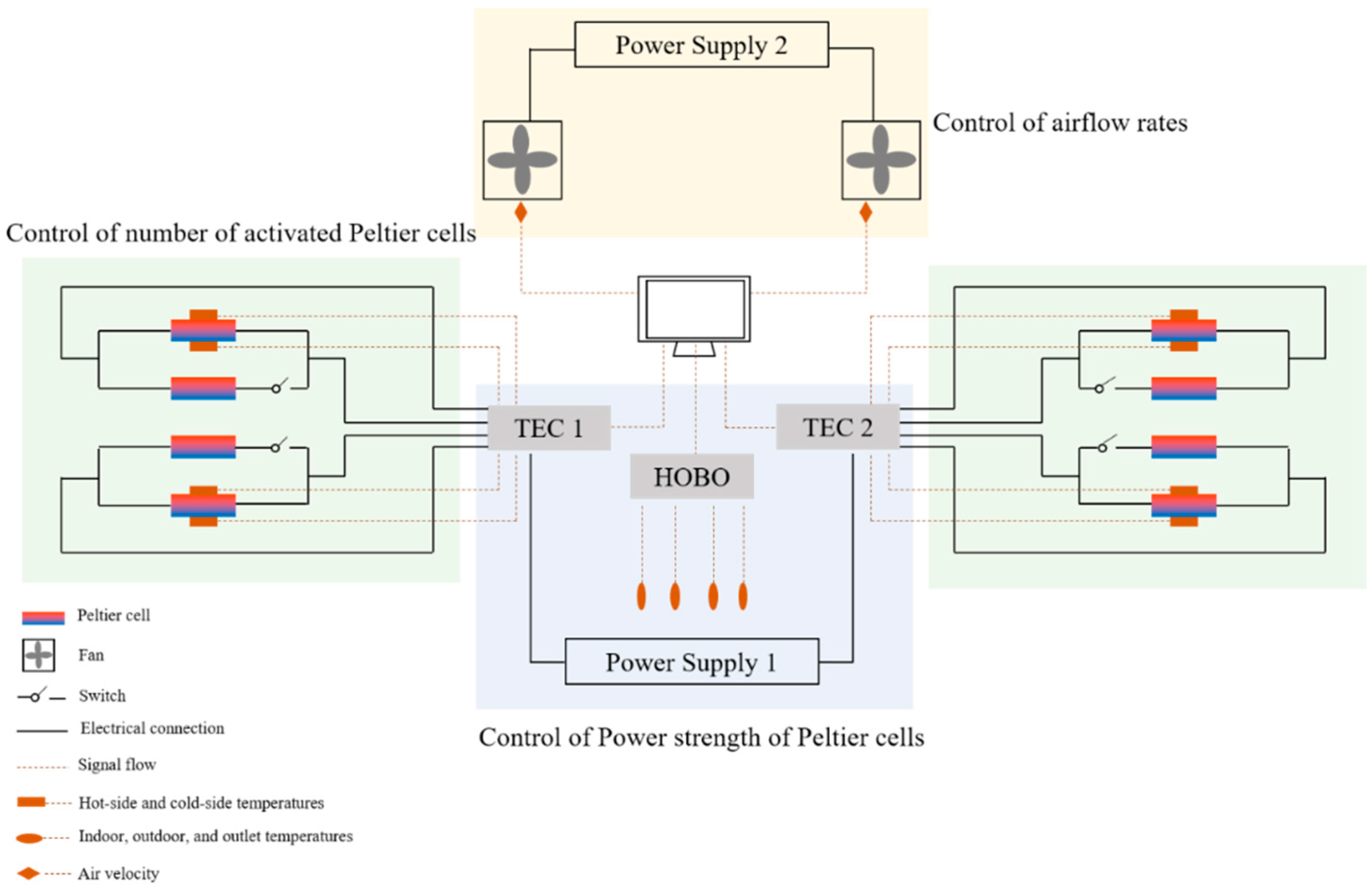
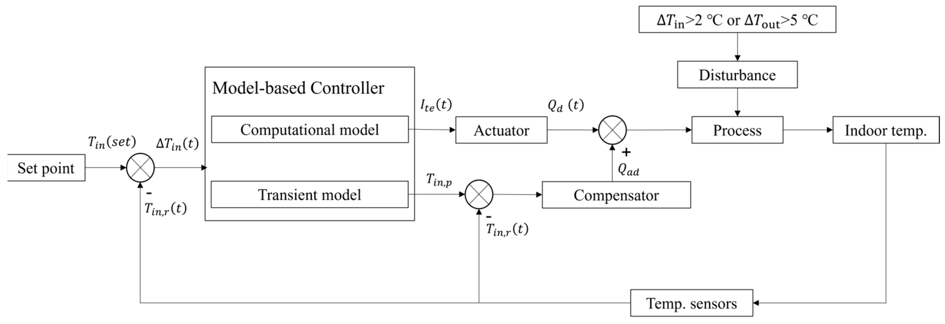
3.3. Control Methodology

As shown in Figure 8, the computational model can calculate the operating current for achieving a certain set point after determining the condition parameters. Following it, the transient model simulates the timewise change in indoor temperature. The TEWF system supplies the required thermal capacity to meet the heat load. During the regulation process, the real-time indoor temperature is compared with the predicted indoor temperature. Consistent deviations between the two indicate a mismatch between the current thermal capacity and the heat load, prompting iterative adjustments by adding additional thermal capacity. If the indoor temperature variation follows the desired temperature profile, the system continues to track the real-time temperature until the target indoor temperature is reached. Additionally, both indoor and outdoor temperature variations are monitored to inform the next regulation update and account for potential disturbances.

Specifically, a model-based control methodology is proposed here based on the models, as shown in Figure 9.

Firstly, the computational model is activated to calculate the operating current after the working condition is defined, as explained in Section 3.1. Then, the transient model is activated to predict the indoor temperature using the calculated operating current and generates the indoor temperature profile. Next, the real-time indoor temperature is continuously compared to the temperature profile. If the deviation between the real-time value and the profile value exceeds 1 °C consistently, it indicates additional heat loss, likely caused by occupant behavior such as opening windows or doors. This additional heat loss means the thermal capacity of the system cannot meet the required thermal demand. Therefore, the thermal capacity is adjusted iteratively based on the deviations between the real-time temperature and the value of the temperature profile by adding the extra heat load until the deviation between the real-time and profile values is reduced to within 1 °C.

After this, the indoor temperature is checked to see whether the set point is achieved. If the deviation between the real-time indoor temperature and the set point exceeds 1 °C, it indicates that the system is still regulating. In this case, the process returns to the previous step and continues to iterate until the deviation is reduced to less than 1 °C, at which point the indoor temperature reaches the desired value. Finally, the system continuously monitors both indoor and outdoor conditions. If there is a significant outdoor temperature change of more than 5 °C (e.g., due to weather fluctuation) or indoor temperature change of 2 °C (e.g., from indoor disturbances), the process restarts to create the desired indoor temperature under the new working condition. Regarding weather conditions, the control method dynamically adjusts to varying weather conditions by continuously monitoring the outdoor temperature and updating the thermal capacity as needed. For long-term applications across different seasons, the system can incorporate historical weather data to anticipate heating or cooling demands, ensuring robust performance under both seasonal and daily fluctuations.

4. Results Analysis and Discussion

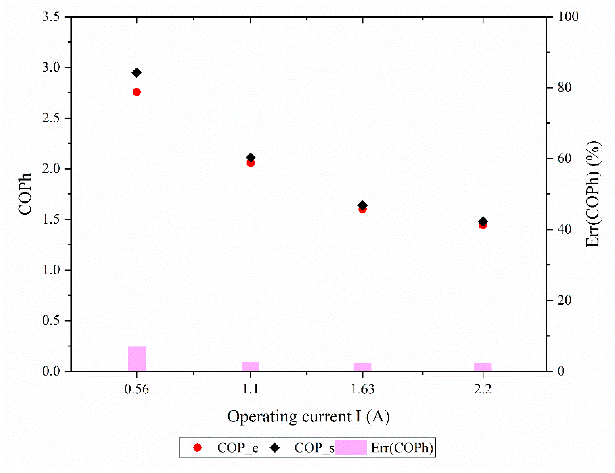
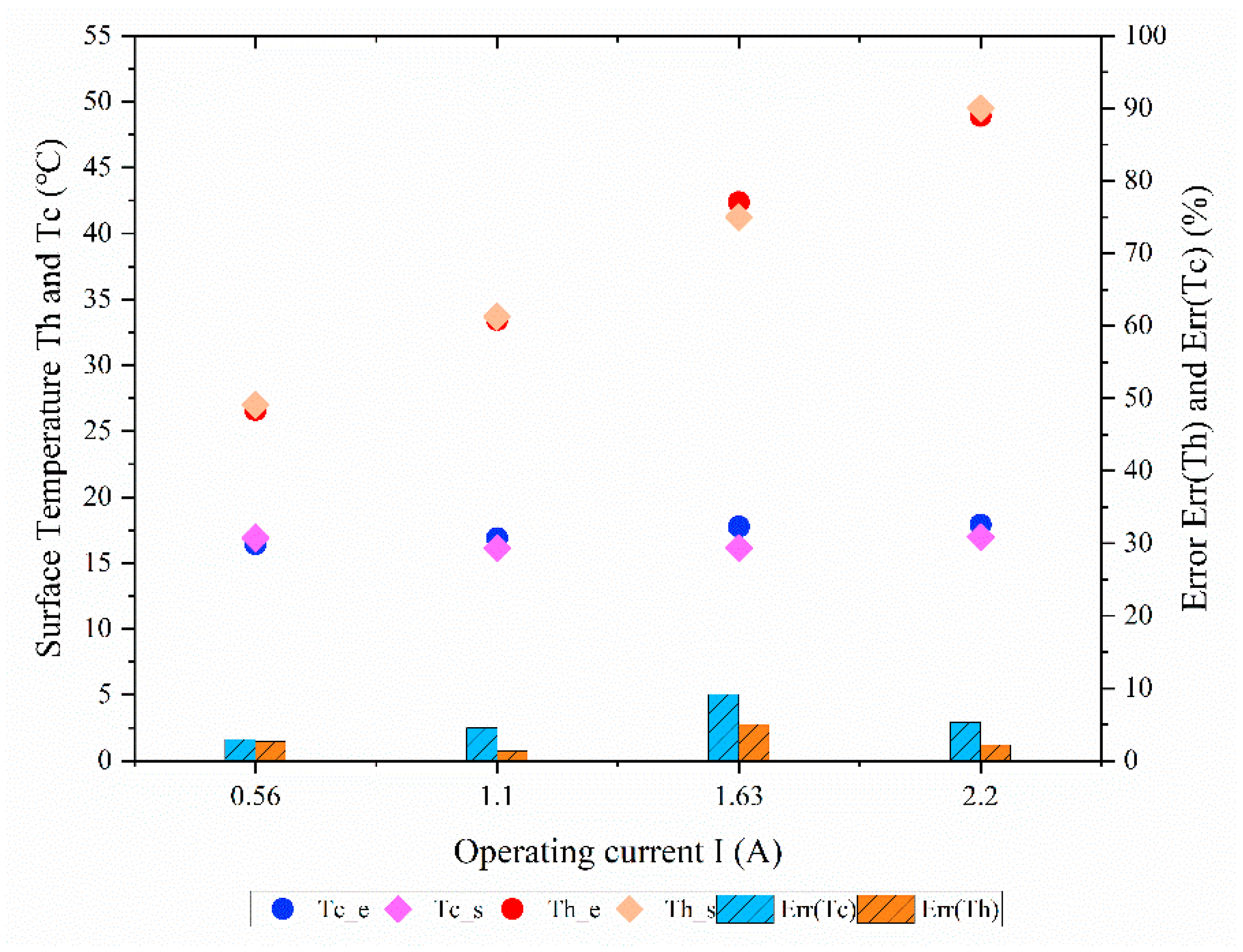
4.1. Operating Current

As mentioned above, the computational model is established to calculate the desired operating currents under certain working conditions. To validate the computational model, the TEWF is operated using the calculated operating currents under different working conditions. Specifically, to achieve indoor temperatures of 22 °C, 24 °C, 26 °C, and 28 °C under an outdoor temperature of 20 °C ± 0.5 °C, operating currents of 0.56 A, 1.1 A, 1.63 A, and 2.2 A are applied. These currents provide heating capacities of 23.8 W, 67.27 W, 112.34 W, and 177 W, respectively, considering a supply air temperature difference of 5 °C.

As shown in Figure 10, the TEWF delivers heating capacities of 21 W, 67 W, 114 W, and 183 W using the calculated operating currents. Furthermore, as shown in Figure 11, experimental data and simulated results for the hot and cold-side temperatures of Peltier cells align closely with a maximal error of 9.2%. These findings reinforce the conclusion from previous work that increasing the operating current enhances the thermal capacity and results in a greater temperature difference between the hot and cold sides [20].

Additionally, the COP_h decreases from 2.75 to 1.45 as the operating current increases from 0.56 A to 2.2 A, with a maximal error of 7%, as shown in Figure 12. Compared to the COP_h of the TEWF with four Peltier cells in previous work [20], the TEWF with eight Peltier cells exhibits improved COP_h at similar operating currents. This further verifies the conclusion that activating more Peltier cells in the range of the optimal number improves the system performance [33].

To assess the accuracy of the computational model, simulation results are compared with experimental data under the specified conditions. The model accuracy is evaluated using the coefficient of variation in the root mean square error CV(RMSE), as defined in Equation (19) [38]. The acceptable tolerances of the CV(RMSE) are within ±15% based on the guidelines of ASHRAE 14 and FEMP [39]. As shown in Figure 8, Figure 9 and Figure 10, the experimental results and simulations of the heating capacities, surface temperatures of Peltier cells, and the COP_h exhibit errors of less than 15%. This demonstrates that there is good accuracy in the computation model.

$$CV\left(RMSE\right)={\displaystyle \frac{1}{\overline{x_e}}}\sqrt{{\displaystyle \frac{\sum _{i=1}^n{\left(x_{ei}-x_{si}\right)}^2}{n}}}\times 100$$

(19)

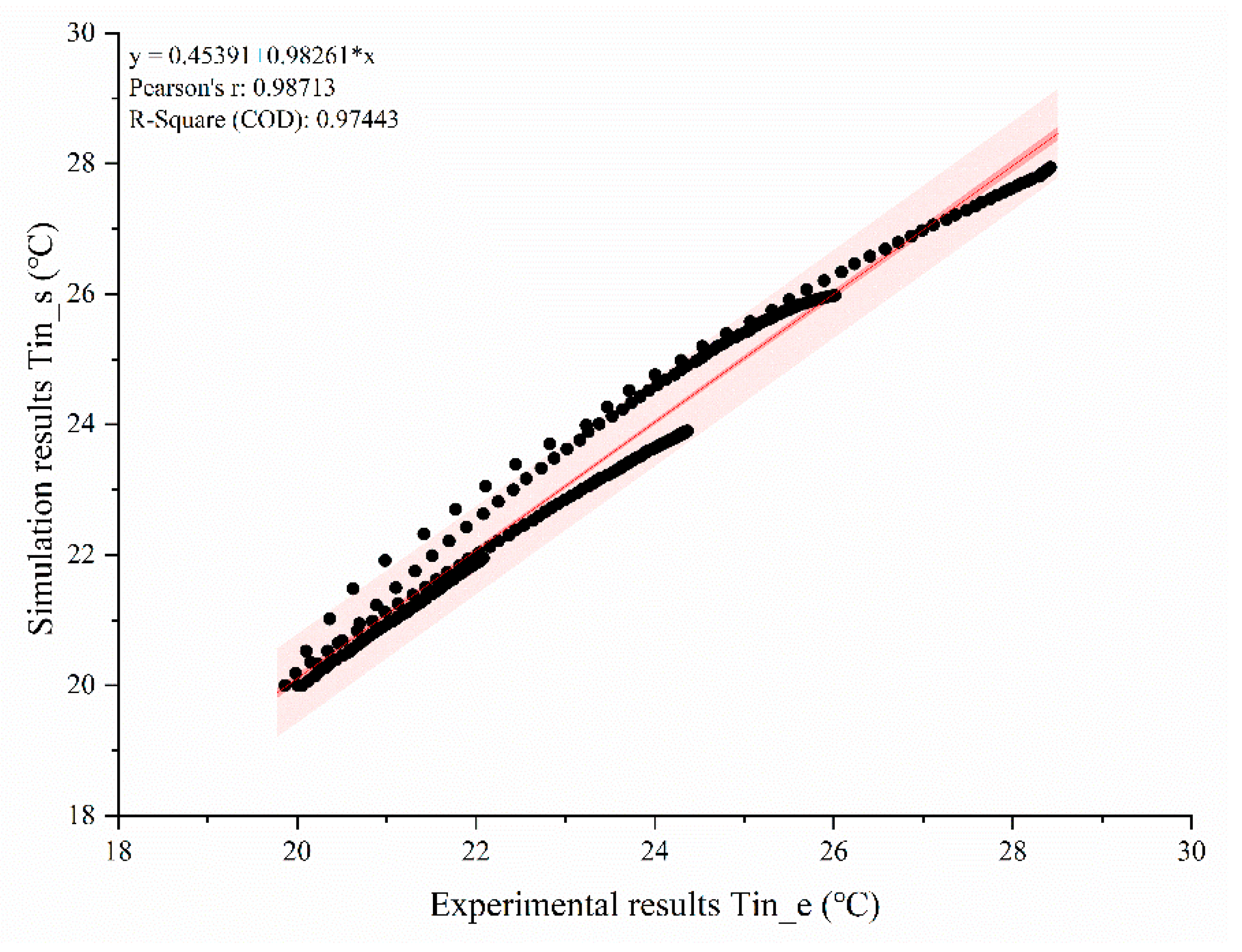
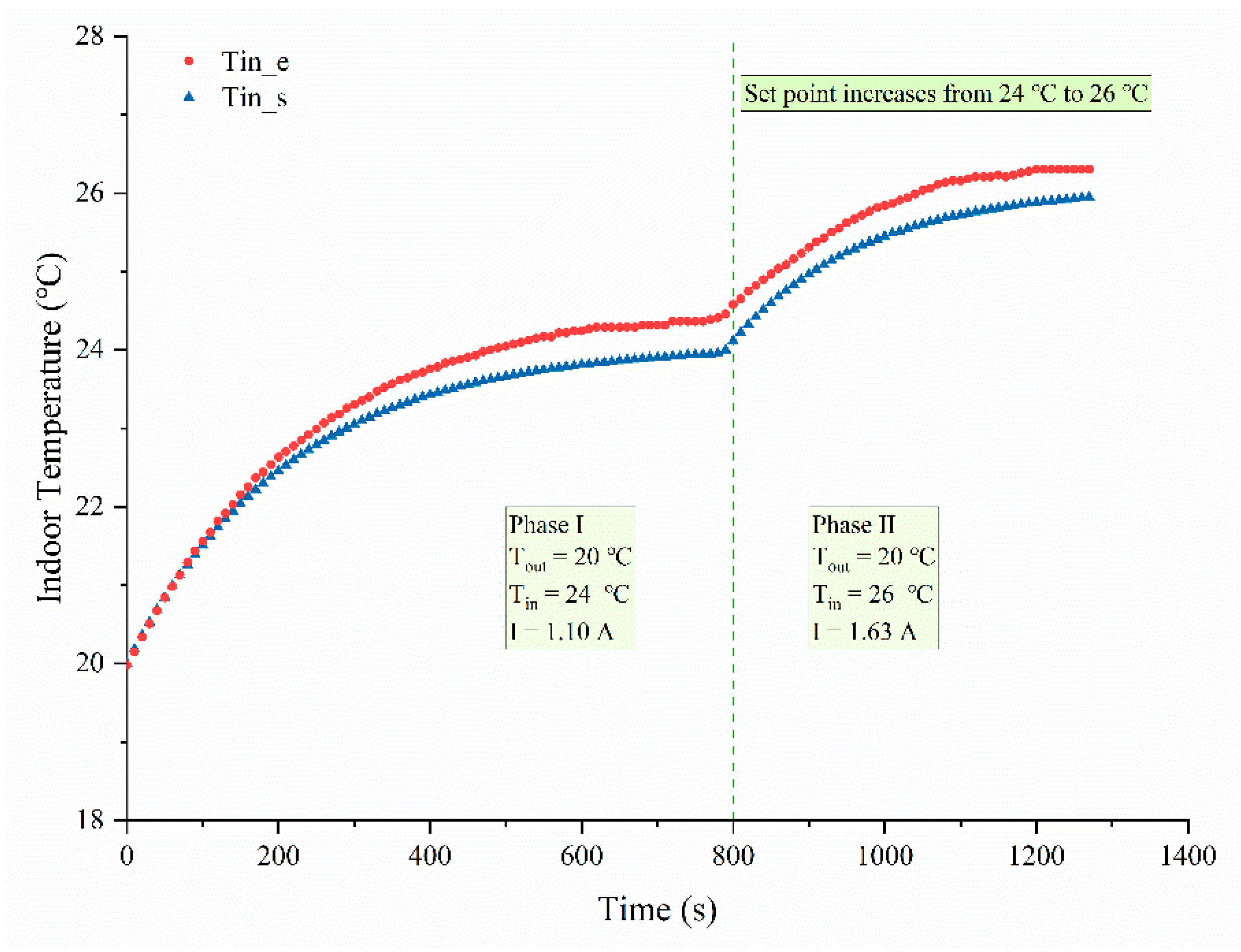
4.2. Indoor Temperature Profile

The variations in indoor temperature of the TEWF over time are also recorded and compared with the operating currents of 0.56 A, 1.1 A, 1.63 A, and 2.2 A under the laboratory ambient of 20 °C ± 0.5 °C. As shown in Figure 13, the TEWF system requires more time to achieve the desired indoor temperature when operating at a lower operating current. Nevertheless, it successfully achieves the set points of 22 °C, 24 °C, 26 °C, and 28 °C. Additionally, the variation profiles of the indoor temperatures from simulations closely match the experimental results with minor deviations.

As shown in Figure 14, most of the errors between the experimental data and simulated indoor temperature are under ±5%. Furthermore, the comparison results reveal that the values of the R-Square and Pearson’s R are 0.97 and 0.98, respectively, indicating a strong linear relationship between the experimental results and simulations. Consequently, the transient model developed in MATLAB R2024a is validated by experimental data. Therefore, the computational and transient models developed in this work can serve to maintain stable indoor temperatures under fluctuating working conditions by calculating the required operating currents and predicting the indoor temperature changes over time. The robustness of the model-based TEWF system, including its ability to handle indoor and outdoor disturbances, will be evaluated in subsequent sections.

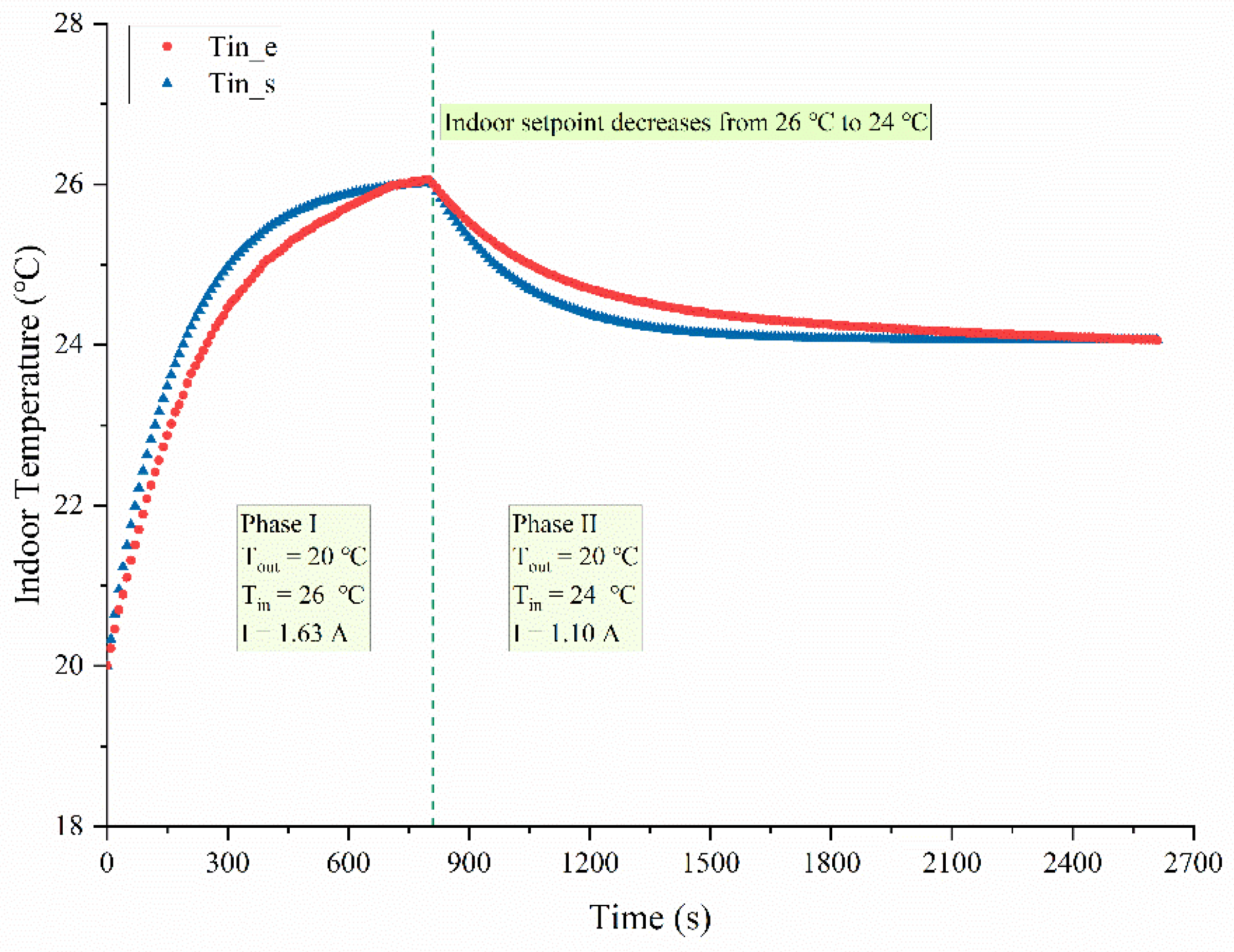
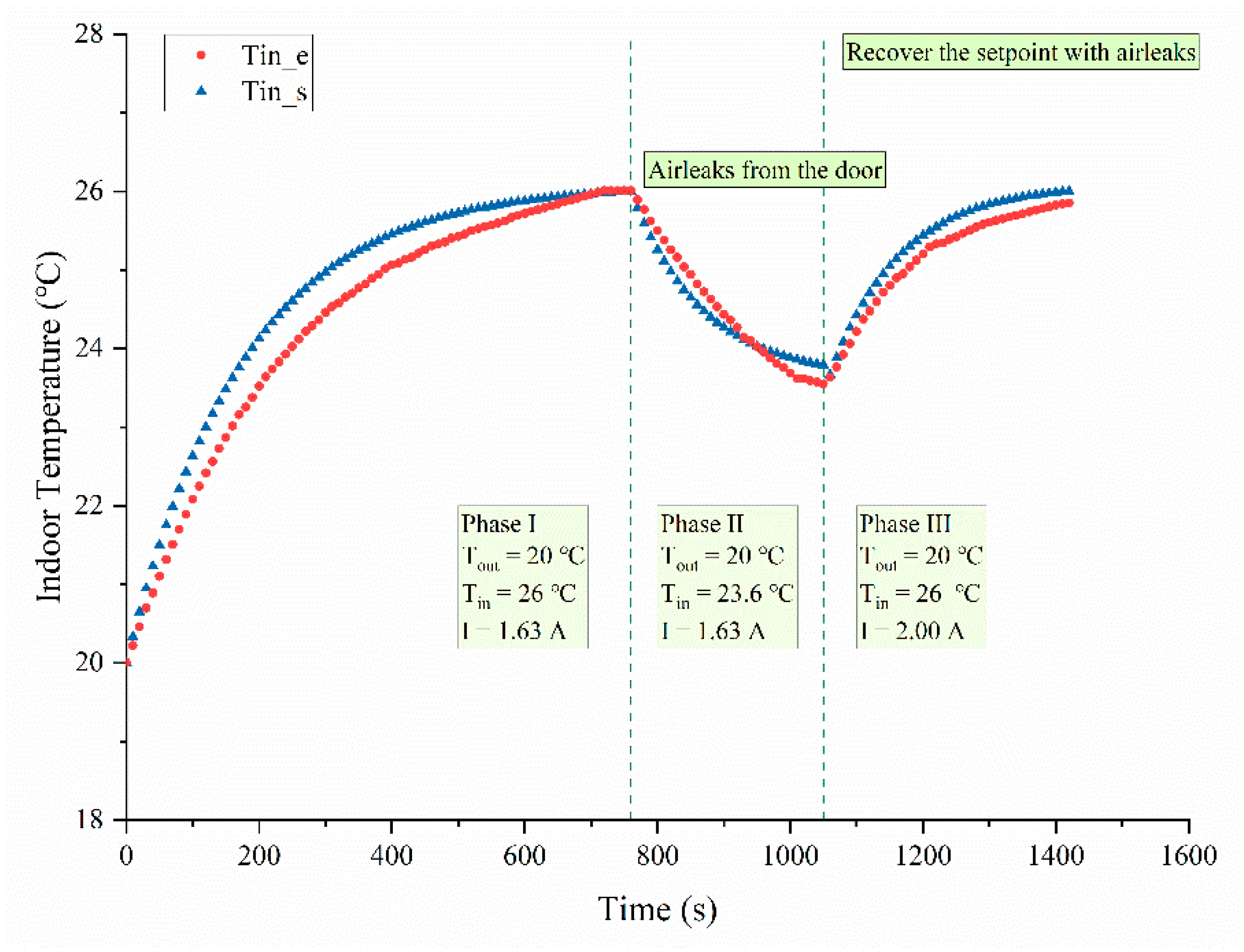
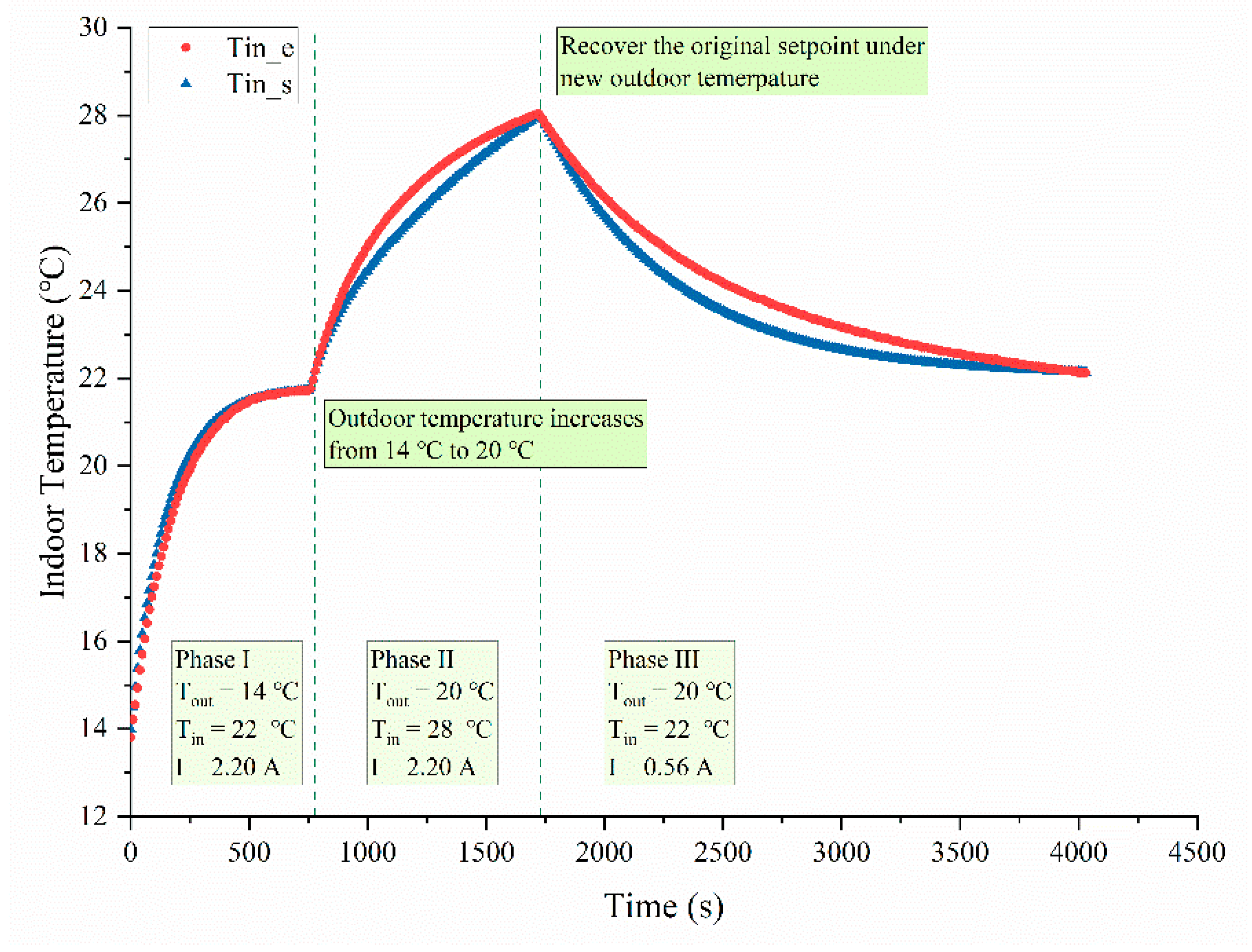
4.3. Responses to Interferences

After verifying the computational model’s ability to determine operating currents under specific working conditions and simulating indoor temperature variation profiles for different set points using the transient model, the model-based control methodology is verified in this section. Indoor temperature profiles are simulated and experimentally assessed under various interferences, including setpoint changes, air leaks, and outdoor temperature fluctuations.

As shown in Figure 15, the operating current of 1.1 A is applied to create an indoor temperature of 24 °C. When the indoor ambience stabilizes at the set point, occupants increase the set point to 26 °C. To reach the new desired indoor temperature, the corresponding operating current is increased to 1.63 A. The indoor temperature generally rises, achieving the set point of 26 °C within 500 s. Conversely, as shown in Figure 16, when the indoor temperature is maintained at 26 °C by applying the operating current of 1.63 A, the set point is lowered to 24 °C. The operating current is decreased to 1.1 A, and the indoor temperature generally falls to 24 °C within 1500 s.

Regarding indoor interferences, except for the changes in the set point, air leaks caused by the occupant’s behavior, such as opening the window or door, are also common. If the provided thermal capacity only meets the heat load under normal conditions, maintaining the desired indoor temperature becomes impossible during air leaks. In this scenario, as described in the control methodology, additional thermal capacity should be provided. Specifically, after the interior temperature of the test box is stabilized at 26 °C, the door is partially opened to simulate an air leak.

As shown in Figure 17, the indoor temperature quickly drops from 26 °C and generally stabilizes at approximately 23.6 °C. To recover the set point of 26 °C with the air leak under the ambient temperature of 20 °C ± 0.5 °C, an additional thermal capacity of 45 W is provided at the 1100th second. Consequently, the operating current increases from 1.63 A to 2 A, and the indoor temperature generally returns to 26 °C within 500 s. The results indicate that when an air leak occurs, the indoor temperature fails to reach the setpoint and ultimately stabilizes at an undesired value. To achieve the desired setpoint, additional thermal capacity must be supplied by adjusting the operating current to accommodate the new conditions caused by the air leak.

Additionally, outdoor interference is also considered in tests. Exactly after the interior ambient of the test box stabilizes at 22 °C with an operating current of 2.2 A under the outdoor ambient with the outdoor temperature of 14 °C, the test box is moved to a laboratory ambient with the outdoor temperature of 20 °C. As shown in Figure 18, without adjusting the operating current, the indoor temperature rises to 28 °C with the operating current of 2.2 A. Furthermore, the new operating current of 0.56 A is applied to test control performance. Consequently, the indoor temperature generally decreases from 28 °C to 22 °C, demonstrating that the calculated operating current can effectively achieve the desired set point. Therefore, fluctuations in outdoor temperature have a significant impact on reaching the indoor setpoint. When the outdoor temperature changes, a new operating current should be applied to compensate for the temperature fluctuation to maintain the set point.

As shown in Figure 19, the deviations between experimental and simulation results in these scenarios are generally within 0 to 5%. Most deviations fall in the range of 1% to 2%, indicating good agreement between the experimental and simulation results. Additionally, while the Peltier cell itself has a rapid electrical response, typically within milliseconds to a few seconds, the overall thermal response of the system is influenced by factors such as the thermal mass of the components, heat dissipation mechanisms, and ambient environmental conditions. In our case, the test box is small and well-insulated, which minimizes heat loss and reduces thermal inertia. As a result, as shown in Figure 15 to Figure 18, the system exhibited a maximal rise time of about 5 min, a maximal settling time of approximately 15 min, and a maximal overshoot of ±3% following sudden temperature changes, reaching steady-state conditions. In conclusion, the computational model effectively provides the required operating currents under specific working conditions, while the transient model accurately simulates indoor temperature change profiles. Experimental results validate the models’ performance and the model-based control methodology applied in the TEWF system. This methodology demonstrates the potential to maintain stable indoor temperatures under various interferences, including set point changes, air leaks, and outdoor temperature fluctuations.

5. Conclusions

The TEWF system serves to regulate the indoor temperature and only occupies the space within the window frames. The thermal capacities of the TEWF system can be adjusted by regulating the operating current to achieve the desired indoor temperature. However, disturbances from indoor and outdoor ambient are inevitable, causing fluctuations in the indoor temperature and preventing it from reaching the set point. To solve the problem, a control system is necessary. In this work, a model-based control method is proposed to maintain the indoor temperature at the set point. This method relies on a computational model for determining the operating current and a transient model for tracking variations in indoor temperature. Additionally, the control methodology is developed to regulate the TEWF system while considering the disturbances mentioned above.

The two models are validated by experimental results under various working conditions. The results show that the operating current calculated by the computation model provides the necessary thermal capacity to reach the set point. The simulated indoor temperature profile closely matches the experimental results, with errors no greater than 15%. Moreover, indoor interference (e.g., changes in set point or air leaks due to occupants’ behavior) and outdoor interference (e.g., change in the outdoor temperature) are incorporated into stable-state experiments. When these interferences occur, new operating currents are calculated for the new working conditions and applied to the TEWF system. Additionally, these interferences can be detected by comparing the real-time indoor temperature profile with the one output by the transient model. The results show that the indoor temperature significantly deviates from the desired values if the operating currents are not adjusted when disturbances occur. However, by regulating the new operating currents in time, the indoor temperature can reach the set point, even during disturbances. The errors are generally in the range of 1% to 2%.

In this work, some research limitations still exist, as follows:

(a)

Regarding the construction of the prototype, due to the existence of the temperature sensors, there is still interspace between Peltier cells and the heat sink, which easily results in extreme surface temperatures and large temperature differences between the hot and cold sides, then negatively affects the COP;

(b)

The experimental booth cannot appropriately simulate the temperature distribution in a real room scale, but the local area near the window;

(c)

This research applies the model-based control to stabilize the indoor temperature with interferences. However, the performance of model-based control heavily depends on the accuracy of the TEWF model. In case that components, such as Peltier cells, fans, or electric elements, wear out over time, the model may need frequent recalibration.

Therefore, from a future perspective, some aspects of TEWF system will be improved.

(a)

Structural optimization. The metal bolts and aluminum frames will be replaced by low-conductivity materials, such as high strength plastic. Additionally, placing strategically sensors for measuring the surface temperature of Peltier cells directly in the subplates (creating dedicated openings for the sensors) will eliminate the space between the subplates and Peltier cells as far as possible. Furthermore, implementing superior insulation between the heat sinks would serve to mitigate heat loss.

(b)

Control method. Several other control methods, including PID control, adaptive PID control, fuzzy logic control, and other model-free control, could be applied and compared with the model-based control method. This comparison would help identify the optimal control strategy for TE systems in buildings.

(c)

Building-scale application. Building-scale experiments of the TEWF can be conducted to assess its actual heating and cooling potential for practical applications. The solutions to decrease non-uniform indoor temperature distribution in the room and increase the thermal capacity of the TEWF should be explored, for example, integrating with a background independent air-conditioning system or TE systems integrated with other construction parts (wall, ceiling, etc.).

References

1. Beretta, D.; Neophytou, N.; Hodges, J.M.; Kanatzidis, M.G.; Narducci, D.; Martin-Gonzalez, M.; Beekman, M.; Balke, B.; Cerretti, G.; Tremel, W.; et al. Thermoelectrics: From history, a window to the future. Mater. Sci. Eng. R Rep. 2019, 138, 210–255. [Google Scholar] [CrossRef]
2. Mannella, G.A.; La Carrubba, V.; Brucato, V. Peltier cells as temperature control elements: Experimental characterization and modeling. Appl. Therm. Eng. 2014, 63, 234–245. [Google Scholar] [CrossRef]
3. Luo, Y.; Zhang, L.; Liu, Z.; Wang, Y.; Meng, F.; Wu, J. Thermal performance evaluation of an active building integratedphotovoltaic thermoelectric wall system. Appl. Energy 2016, 177, 25–39. [Google Scholar] [CrossRef]
4. Martín-Gómez, C.; Zuazua-Ros, A.; Del Valle de Lersundi, K.; Sánchez Saiz-Ezquerra, B.; Ibáñez-Puy, M. Integration development of a ventilated active thermoelectric envelope (VATE): Constructive optimization and thermal performance. Energy Build. 2021, 231, 110593. [Google Scholar] [CrossRef]
5. Wang, P.; Liu, Z.; Chen, D.; Li, W.; Zhang, L. Experimental study and multi-objective optimisation of a novel integral thermoelectric wall. Energy Build. 2021, 252, 111403. [Google Scholar] [CrossRef]
6. Birthwright, R.-S.; Messac, A.; Harren-Lewis, T.; Rangavajhala, S. Heat compensation in buildings using thermoelectric windows: An energy efficient window technology. In Proceedings of the ASME 2008 International Design Engineering Technical Conferences and Computers and Information in Engineering Conference, Brooklyn, NY, USA, 3–6 August 2008; pp. 977–987. [Google Scholar] [CrossRef]
7. Xu, X.; Van Dessel, S. Evaluation of an active building envelope window-system. Build Environ. 2008, 43, 1785–1791. [Google Scholar] [CrossRef]
8. Luo, Y.; Zhang, L.; Liu, Z.; Wang, Y.; Meng, F.; Xie, L. Modeling of the surface temperature field of a thermoelectric radiant ceiling panel system. Appl. Energy 2016, 162, 675–686. [Google Scholar] [CrossRef]
9. Seyednezhad, M.; Najafi, H. Numerical analysis and parametric study of a thermoelectric-based radiant ceiling panel for building cooling applications. In Proceedings of the ASME 2020 International Mechanical Engineering Congress and Exposition, Online, 16–19 November 2020; Volume 8. [Google Scholar] [CrossRef]
10. Diaz de Garayo, S.; Martínez, A.; Astrain, D. Optimal combination of an air-to-air thermoelectric heat pump with a heat recovery system to HVAC a passive house dwelling. Appl. Energy 2022, 309, 118443. [Google Scholar] [CrossRef]
11. Zuazua-Ros, A.; Martín-Gómez, C.; Ibañez-Puy, E.; Vidaurre-Arbizu, M.; Gelbstein, Y. Investigation of the thermoelectric potential for heating, cooling and ventilation in buildings: Characterization options and applications. Renew. Energy 2019, 131, 229–239. [Google Scholar] [CrossRef]
12. Liu, Z.; Zhang, L.; Gong, G.; Luo, Y.; Meng, F. Evaluation of a prototype active solar thermoelectric radiant wall system in winter conditions. Appl. Therm. Eng. 2015, 89, 36–43. [Google Scholar] [CrossRef]
13. Cheng, T.-C.; Cheng, C.-H.; Huang, Z.-Z.; Liao, G.-C. Development of an energy-saving module via combination of solar cellsand thermoelectric coolers for green building applications. Energy 2011, 36, 133–140. [Google Scholar] [CrossRef]
14. Seyednezhad, M.; Najafi, H. Solar-powered thermoelectric-based cooling and heating system for building applications: A parametric study. Energies 2021, 14, 5573. [Google Scholar] [CrossRef]
15. Diaz-Londono, C.; Enescu, D.; Ruiz, F.; Mazza, A. Experimental modeling and aggregation strategy for thermoelectric refrigeration units as flexible loads. Appl. Energy 2020, 272, 115065. [Google Scholar] [CrossRef]
16. Duan, M.; Sun, H.; Lin, B.; Wu, Y. Evaluation on the applicability of thermoelectric air cooling systems for buildings with thermoelectric material optimization. Energy 2021, 221, 119723. [Google Scholar] [CrossRef]
17. Khire, R.A.; Messac, A.; Van Dessel, S. Optimization based design of thermoelectric heat pump unit of active building envelope systems. In Proceedings of the ASME 2005 International Mechanical Engineering Congress and Exposition, Orlando, Fl, USA, 5–11 November 2005; pp. 161–173. [Google Scholar] [CrossRef]
18. Kim, Y.W.; Ramousse, J.; Fraisse, G.; Dalicieux, P.; Baranek, P. Optimal sizing of a thermoelectric heat pump (THP) for heatingenergy-efficient buildings. Energy Build. 2014, 70, 106–116. [Google Scholar] [CrossRef]
19. He, Z.; Zuazua-Ros, A.; Martín-Gómez, C. Thermoelectric system applications in buildings: A review of key factors and control methods. J. Build. Eng. 2023, 78, 107658. [Google Scholar] [CrossRef]
20. He, Z.; Zuazua-Ros, A.; Martín-Gómez, C. Current-dependent temperature change model of a thermoelectric window frame. Appl. Therm. Eng. 2024, 247, 123081. [Google Scholar] [CrossRef]
21. Keshtkar, A.; Arzanpour, S. An adaptive fuzzy logic system for residential energy management in smart grid environments. Appl. Energy 2017, 186, 68–81. [Google Scholar] [CrossRef]
22. Güler, N.F.; Ahiska, R. Design and testing of a microprocessor-controlled portable thermoelectric medical cooling kit. Appl. Therm. Eng. 2002, 22, 1271–1276. [Google Scholar] [CrossRef]
23. Chojecki, A.; Ambroziak, A.; Borkowski, P. Fuzzy controllers instead of classical pids in hvac equipment: Dusting off a well-known technology and today’s implementation for better energy efficiency and user comfort. Energies 2023, 16, 2967. [Google Scholar] [CrossRef]
24. Li, Y.; Bian, J.; Zhang, N.; Li, J. Experimental study on intelligent control scheme for fan coil air-conditioning system. Adv. Mech. Eng. 2013, 5, 481213. [Google Scholar] [CrossRef]
25. Işik, H.; Saraçoğlu, E. The design of thermoelectric footwear heating system via fuzzy logic. J. Med. Syst. 2007, 31, 521–527. [Google Scholar] [CrossRef] [PubMed]
26. Ahiska, R.; Yavuz, A.H.; Kaymaz, M.; Güler, I. Control of a thermoelectric brain cooler by adaptive neuro-fuzzy inference system. Instrum. Sci. Technol. 2008, 36, 636–655. [Google Scholar] [CrossRef]
27. Wang, J.; Wang, Y.; Qiu, D.; Su, H.; Strbac, G.; Gao, Z. Resilient energy management of a multi-energy building under low-temperature district heating: A deep reinforcement learning approach. Appl. Energy 2025, 378, 124780. [Google Scholar] [CrossRef]
28. Wang, Y.; Qiu, D.; Sun, X.; Bie, Z.; Strbac, G. Coordinating multi-energy microgrids for integrated energy system resilience: A multi-task learning approach. IEEE Trans. Sustain. Energy 2024, 15, 920–937. [Google Scholar] [CrossRef]
29. Luo, J.; Lee, J. Machine learning-assisted thermoelectric cooling for on-demand multi-hotspot thermal management. J. Appl. Phys. 2024, 135, 244503. [Google Scholar] [CrossRef]
30. Kishore, M.; Sharma, B.; Pillai, B.M.; Suthakorn, J. Model predictive control-based thermoelectric cooling for rough terrain rescue robots. IEEE Access 2021, 9, 167652–167662. [Google Scholar] [CrossRef]
31. Wang, R.; Zhang, H.; Chen, J.; Ding, R.; Luo, D. Modeling and model predictive control of a battery thermal management system based on thermoelectric cooling for electric vehicles. Energy Technol. 2024, 12, 2301205. [Google Scholar] [CrossRef]
32. Kajgaard, M.U.; Mogensen, J.; Wittendorff, A.; Veress, A.T.; Biegel, B. Model predictive control of domestic heat pump. In Proceedings of the 2013 American Control Conference, Washington, DC, USA, 17–19 June 2013. [Google Scholar] [CrossRef]
33. He, Z.; Zuazua-Ros, A.; Martín-Gómez, C. Optimizing a thermoelectric window frame for heating and cooling: A cross-validated simulation study. Build. Simul. 2024, 17, 2355–2372. [Google Scholar] [CrossRef]
34. Arias-Salazar, P.; Zuazua-Ros, A.; Sacristán-Fernández, J.A.; He, Z.; Vidaurre-Arbizu, M.; Martín-Gómez, C. Thermoelectric active window frame: Constructive integration and preheating analysis. J. Build. Eng. 2024, 94, 109888. [Google Scholar] [CrossRef]
35. Meerstetter. TEC Controllers|Peltier Controllers n.d. Available online: https://www.meerstetter.ch/products/tec-controllers (accessed on 15 September 2024).
36. HOBO. Temperature Data Loggers n.d. Available online: https://www.onsetcomp.com/products/data-loggers-sensors/temperature (accessed on 15 September 2024).
37. Mills, A.F. Heat Transfer; CRC Press: Boca Raton, FL, USA, 1992. [Google Scholar]
38. Afram, A.; Janabi-Sharifi, F. Black-box modeling of residential HVAC system and comparison of gray-box and black-box modeling methods. Energy Build. 2015, 94, 121–149. [Google Scholar] [CrossRef]
39. Shailza. Energy modeling of multi-storied residential buildings—A manual calibration approach. In Proceedings of the 2018 Building Performance Analysis Conference and SimBuild Co-Organized by ASHRAE and IBPSA-USA, Roorkee, India, 26–28 September 2018; pp. 550–557. [Google Scholar]
Figure 1. The schematic of the system integration and the TEWF.
Buildings 15 01364 g001
Figure 2. The integration of the TEWF with the experimental booth.
Buildings 15 01364 g002
Figure 3. Physical electric system of the TEWF.
Buildings 15 01364 g003
Figure 4. The schematic of the electric control system of the TEWF.
Buildings 15 01364 g004
Figure 5. The block diagram of the computation model of the TEWF in the heating process.
Buildings 15 01364 g005
Figure 6. The flow chart of the computational model for the operating current of the TEWF in the heating process.
Buildings 15 01364 g006
Figure 7. The schematic of the heat transfer of the TEWF in the heating process.
Buildings 15 01364 g007
Figure 8. The block diagram of the control methodology for the TEWF in the heating process.
Buildings 15 01364 g008
Figure 9. The flow chart of the control methodology for the TEWF in the heating process.
Buildings 15 01364 g009
Figure 10. Comparison of experimental and simulated heating capacities and errors across calculated operating currents.
Buildings 15 01364 g010
Figure 11. Comparison of experimental and simulated surface temperatures and errors across calculated operating currents.
Buildings 15 01364 g011
Figure 12. Comparison of experimental and simulated COPh and errors across calculated operating currents.
Buildings 15 01364 g012
Figure 13. Comparison of experimental and simulated timewise variations in indoor temperatures at calculated operating currents. (a): Timewise variation in indoor temperature under the operation current of 0.56 A; (b): Timewise variation in indoor temperature under the operation current of 1.1 A; (c): Timewise variation in indoor temperature under the operation current of 1.63 A; (d): Timewise variation in indoor temperature under the operation current of 2.2 A.
Buildings 15 01364 g013
Figure 14. Error analysis of timewise variations in indoor temperatures under various set points (* in the figure means multiple sign).
Buildings 15 01364 g014
Figure 15. Timewise variations in indoor temperatures during set point adjustment from 24 °C to 26 °C.
Buildings 15 01364 g015
Figure 16. Timewise variations in indoor temperatures during set point adjustment from 26 °C to 24 °C.
Buildings 15 01364 g016
Figure 17. Timewise variations in indoor temperatures with air leak and operating current compensation.
Buildings 15 01364 g017
Figure 18. Timewise variations in indoor temperatures with outdoor temperature change and operating current compensation.
Buildings 15 01364 g018
Figure 19. Error analysis of timewise variations in indoor temperatures in Figure 15, Figure 16, Figure 17 and Figure 18.
Buildings 15 01364 g019