
Machine Learning Modeling for Building Energy Performance Prediction Based on Simulation Data: A Systematic Review of the Processes, Performances, and Correlation of Process-Related Variables


Abstract
1. Introduction
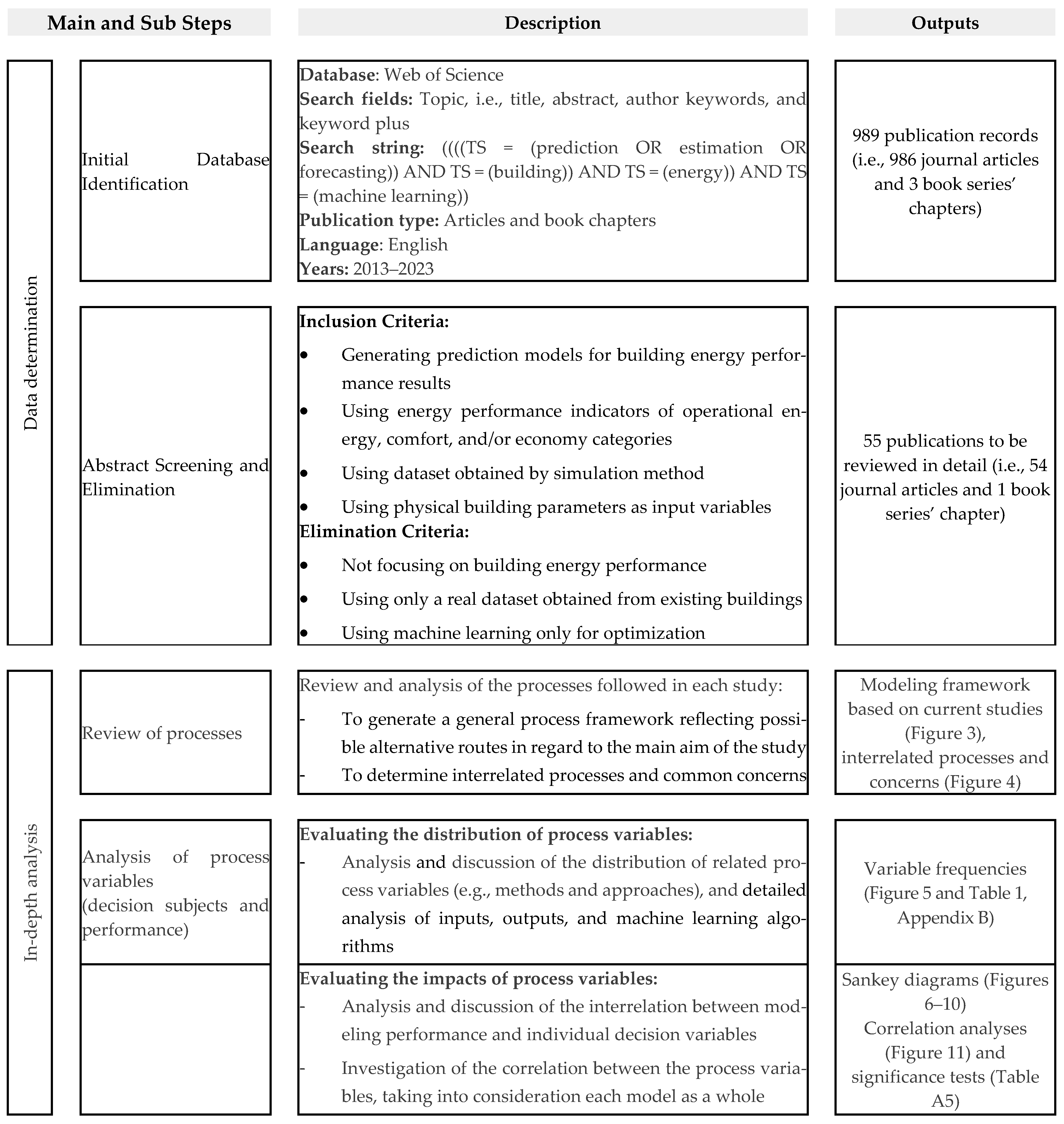
2. Methodology
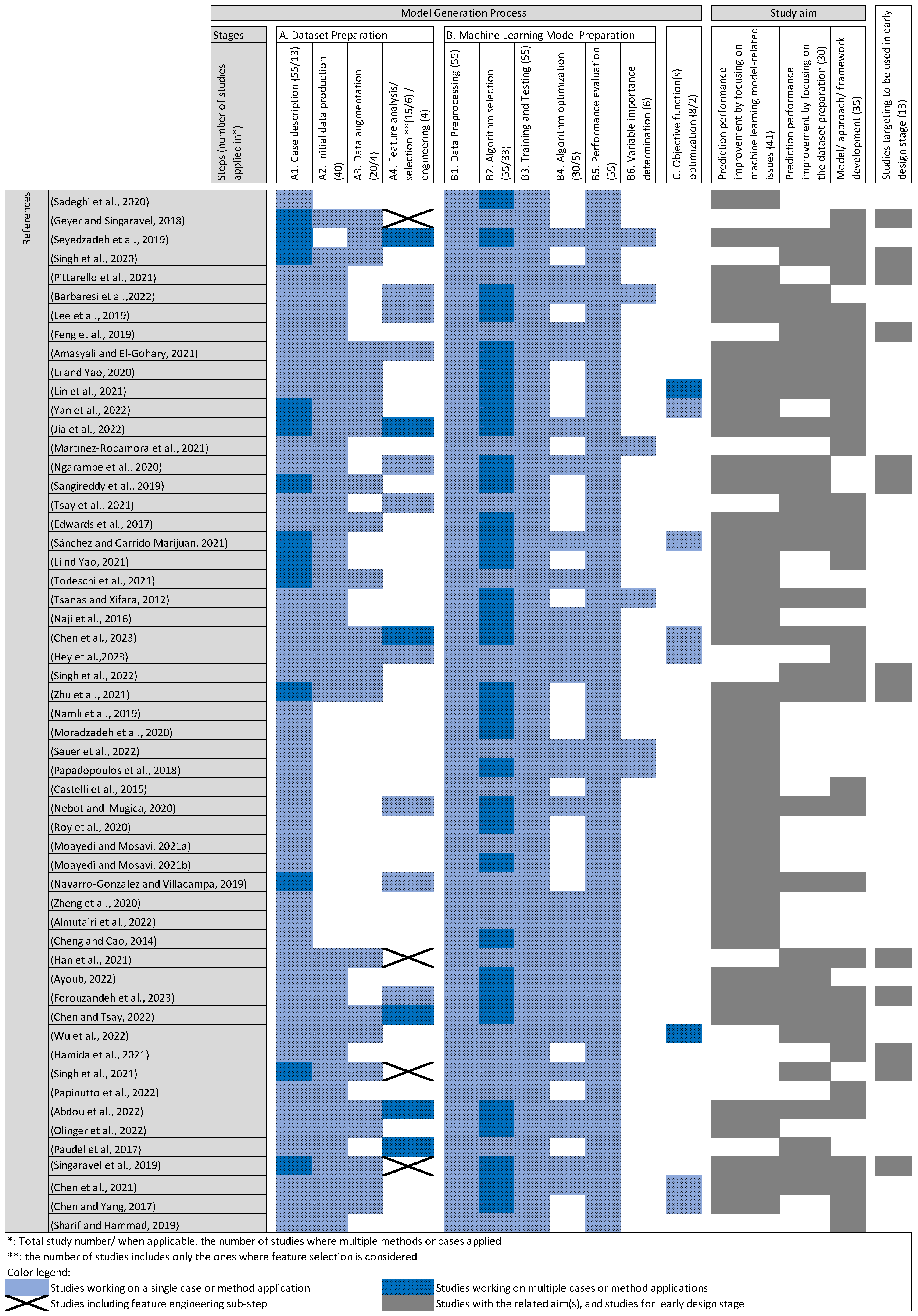
3. Machine Learning Modeling Process in Building Energy Performance Prediction
- (i)
- Improving the prediction performance by focusing on the dataset preparation stage;
- (ii)
- Improving the prediction performance by focusing on issues related to the machine learning model preparation stage;
- (iii)
- (i)
- The dimensionality between the representation of data sufficiently and handling complexity;
- (ii)
- The uncertainty regarding the accuracy of predictions compared to the real building energy consumption/impact results that are affected by factors such as the use of appropriate tools together with sufficient knowledge of simulation modeling, the wide range of probable building design options with a lack of detailed information about them in the design stages considered, the performance of the machine learning algorithm used, etc.;
- (iii)
- The appropriate ensemble of approaches or methods.
3.1. Dataset Preparation
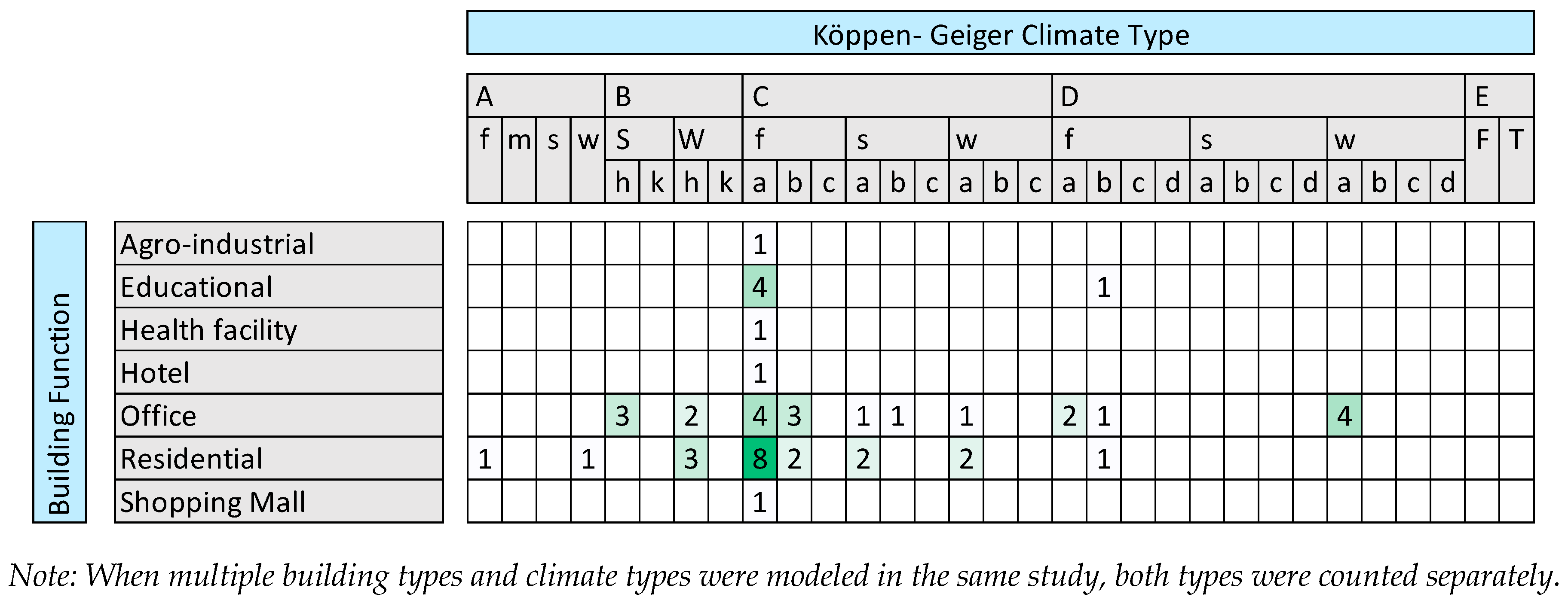
3.1.1. Case Description
3.1.2. Data Production by Simulation
3.1.3. Data Augmentation
3.1.4. Feature Selection and Feature Engineering
3.2. Machine Learning Prediction Model Preparation
3.2.1. Machine Learning Algorithm Selection
3.2.2. Training and Testing
3.2.3. Algorithm Optimization
3.2.4. Performance Evaluation
4. Discussion
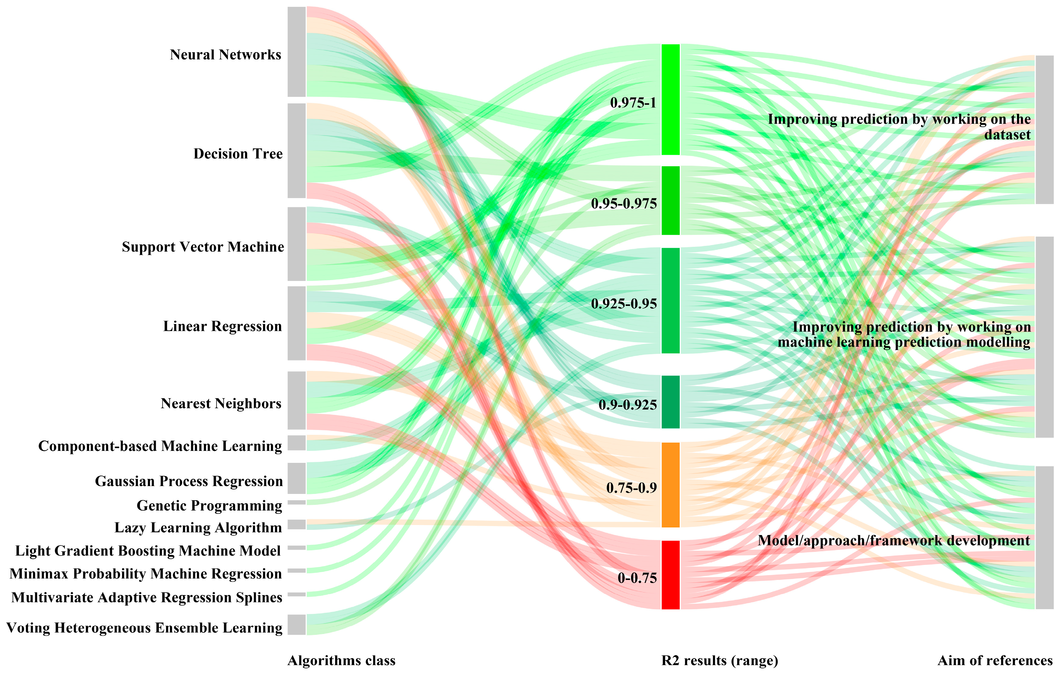
4.1. Correlation of Process-Related Variables
4.2. Strategies Implemented to Overcome Concerns
4.3. Future Directions
5. Conclusions
Author Contributions
Funding
Conflicts of Interest
Appendix A. Prisma Flow Diagram

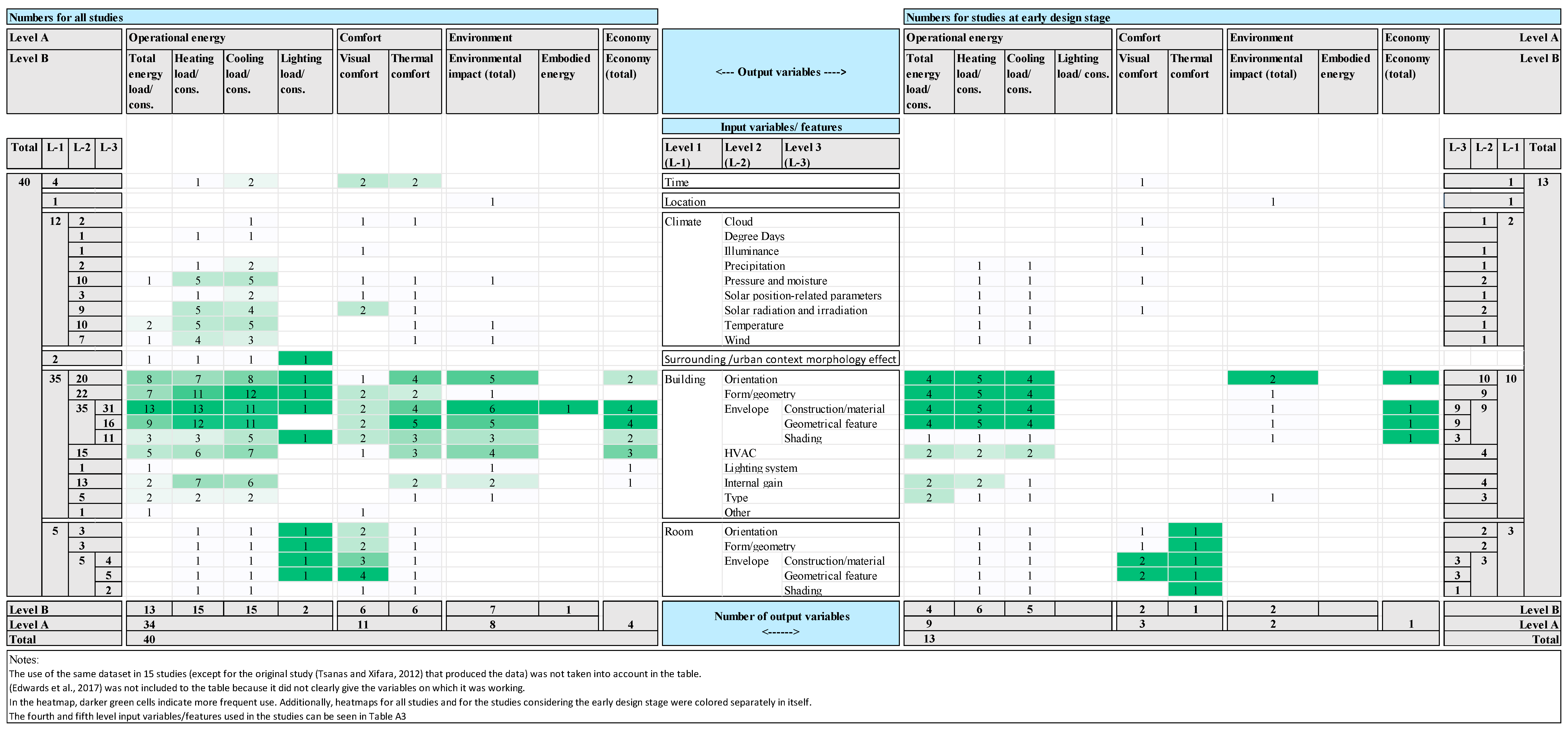
Appendix B. Machine Learning Modeling-Related Information of the Studies Analyzed

| Ref. No | Building Function(s) | City/Country (Climate Type) | Sampling Method(s) | Sample Size: All * | Feature Analysis Method(s) | ML Algorithm(s) | ML Algorithm Optimization Method(s) | Evaluation Metric(s) |
|---|---|---|---|---|---|---|---|---|
| [1] | Residential ** | Athens/Greece (Cfa) ** | No sampling | 768 | Local sensitivity analysis, Global sensitivity analysis | DNN, ANN | N/S | R2, RMSE, MAE, prediction interval (PI) |
| [2] | Office | N/S | Latin hypercube | (800), (200),(200) | Pearson correlation | ANN | N/S | R2, Maximum deviation |
| [5] | Residential ** | Athens/Greece (Cfa) ** | 768 | N/S | ANN, SVM, GPR, RF, GBRT, XGBoost | Grid search | RMSE, MAE, R2, Fit time, Test time, the average fitting time of all tested models | |
| [5] | Various types (health facility, residential, hotel, office, restaurant, retail, educational, warehouse) | Various cities/United States (N/S) | N/S | 1000, 10,000, 25,000 100,000 | Correlation estimation, Principal Component Analysis, Sobol Method | ANN, SVM, GPR, RF, GBRT, XGBoost | Grid search | RMSE, MAE, R2, Fit time, Test time, the average fitting time of all tested models |
| [6] | Office | Munich/Germany (Cfb) | N/S | 4000 | CBML | N/S | R2, RMSE | |
| [8] | Residential | Po Valley area/Italy (Cfa) | No sampling | 600,000 | ANN | Manual | Distribution of the relative errors | |
| [9] | Agro-industrial building (a winery building) | Toscanella di Dozza, in the countryside close to Bologna/Italy (Cfa) | No sampling | 5150 | Spearman correlation | SVR, RF, LR, XGBoost | Grid search | Computational time, MAE, MSE, R2 |
| [12] | Office spaces | Champaign/United States (Dfa) | No sampling | 300 | Principal component analysis | LR, SLR, GAM | N/S | RMSE |
| [28] | Office | Harbin/China (Dwa), Chengdu/China (Cwa) | No sampling | 1152 | ELM | Particle swarm optimization | R2 | |
| [29] | Office | Phoenix/United States(BWh), Houston/United States (Cfa), San Jose/United States (Csb), New York/United States (Cfa), Chicago/United States (Dfa) | Latin hypercube | 1000, 2000, 5000, 10,000, 20,000, 50,000, 100,000, 200,000, 500,000, 1,000,000 | Neighborhood component analysis | CART, ANN, EBT, DNN | Grid search | CV, RMSE, R2, training time |
| [30] | Residential | Chongqing/China (Cfa) | N/S | 50, 100, 150, 200, 250, 300, 400, 500 | Spearman correlation | LR, ANN, SVR | Argument tunelength for the train function in the caret package | MAE, RMSE, NMAE, NRMSE |
| [31] | Residential | Shanghai/China (Cfa) | Latin hypercube | 800 | SLR, BPNN, SVM, RF | N/S | R2, relative error ranges | |
| [32] | Residential | Singapore (Af) | Latin hypercube | 2500 | Pearson correlation | LR, LSTM, MLP, XGBoost | N/S | R2, MSE, MAE |
| [33] | Residential (high-rise buildings) | Lusail city/Qatar (BWh) | Latin hypercube | 585, 1755, 2925, 5850, 8775 | Standardized regression coefficient, Random forest variable importance, T-value, sensitivity value index | MLR, SVR, ANN, XGBoost | Manual | R2, NMBE, CV(RMSE) %, Process time (s) |
| [34] | Residential | Seville/Spain (Csa) | No sampling | 240 | Correlation coefficient | RF | N/S | R2, MAE, RMSE, OOB (Out-of-bag) |
| [35] | N/S | N/S | No sampling | 421,245 | The deep learning methods described by Garson | LSTM, GLM, DNN, RF, GBRT | Adaptive moment estimation | RMSE, MAE, R2 |
| [36] | Office | Jaipur/India (BSh), Hyderabad/India (BWh) | Domain knowledge based sampling, Sampling by clustering | (2400), (2304) | LR, RR, LASSO, RANSAC, Theil Sen, KNN, SVR, DT | N/S | r (Spearman’s rank correlation coefficient), MAPE, error analysis, residual analysis | |
| [37] | Residential | Taipei/Taiwan (Cfa), Taichung/Taiwan (Cwa), Kaohsiung/Taiwan (Aw) | No sampling | 8184 | Spearman correlation index | GBRT | N/S | RMSE, percentage error, R2 |
| [39] | Various types (residential, kindergarten, school) | Belgrade/Serbia (Cfa) | No sampling | not clear | SVR, ANN | Grid search | R2 | |
| [40] | Various types (residential and non-residential buildings [office, hotel, mall, hospital, educational]) | Chongqing/China (Cfa) | No sampling | N/S | SVR, RF, XGBoost, OLS, RR, LASSO, EN, ANN | N/S | NMAE, NRMSE, relative error | |
| [41] | Various types (mainly residential) | Fribourg/Switzerland (Dfb) | Morris method | N/S | Morris method | LGBM | Root mean square propagation | MAE, MAPE |
| [42] | Residential | Athens/Greece (Cfa) | No sampling | 768 | IRLS, RF | N/S | MAE, MSE, MRE | |
| [43] | Residential | Istanbul/Turkey (Cfa) | No sampling | 180 | ELM, GP, ANN | manual | RMSE, R2, Pearson coefficient | |
| [44] | Office | Shandong/China (Dwa) | Fourier amplitude sensitivity test, Sobol sampling, Random sampling, Orthogonal experiment, Latin hypercube | 16,320 | FAST extend, Sobol method, standardized correlation coefficients, Standardized rank correlation coefficients, partial correlation coefficient, partial rank correlation coefficient, Spearman correlation coefficient, Pearson correlation coefficient, Kolmogorov–Smirnov | RF, GBRT, ANN | Randomized search, Grid search | MAE, RMSE, R2 |
| [45] | Residential | Nottingham/United Kingdom (Cfb) | Latin hypercube | 40,000 | A backwards feature selection proces | ANN | Grid search | MAE, residual analysis |
| [46] | Office | N/S | Sobol sampling | 26,000 | A regression-based method | CNN | Manual | MAPE, RMSE |
| [47] | Office | Beijing/China (Dwa) | Latin hypercube | 4740, 4990, 5490, 5990, 7490, 8990 | ANN, RF, GPR, SVM, DACE, MARS | N/S | R2 | |
| [48] | Residential ** | Athens/Greece (Cfa) ** | No sampling | 768 | MLP, SVR, Ibk, LWL, M5P, REPTree | N/S | R2, MAE, RMSE | |
| [49] | Residential ** | Athens/Greece (Cfa) ** | No sampling | 768 | SVR, MLP | N/S | Correlation coefficient (r), MSE, RMSE, MAE | |
| [50] | Residential ** | Athens/Greece (Cfa) ** | No sampling | 768 | XGBoost | Ant Lion Optimizer, Black Hole Optimizer, Cuckoo Search, Dragonfly Algorithm, Differential Evolution, Genetic Algorithm, Gray Wolf Optimizer, Jaya, Particle Swarm Optimization, Modified Jaya | RMSE, R2, MAE | |
| [51] | Residential ** | Athens/Greece (Cfa) ** | No sampling | 768 | Pearson correlation | RF, ERT, GBRT | Grid search | MSE, MAE, MAPE |
| [52] | Residential ** | Athens/Greece (Cfa) ** | No sampling | 768 | GP | Local search method, Linear scaling | MAE, MRE, MSE | |
| [53] | Residential ** | Athens/Greece (Cfa) ** | No sampling | 768 | Fuzzy Inductive Reasoning mask | FIR, ANFIS | A combination of backpropagation and least-squares estimation | RMSE, MAE, SI (a synthesis index = combination of RMSE and MAE measures) |
| [54] | Residential ** | Athens/Greece (Cfa) ** | No sampling | 768 | DNN, GBRT, GPR, MPMR, GPR, LR, ANN, RBFNN, SVM | N/S | VAF, RAAE, RMAE, R2, RSR, NMBE, MAPE, NS, RMSE, WMAPE. | |
| [55] | Residential ** | Athens/Greece (Cfa) ** | No sampling | 768 | MLP | The grasshopper optimization algorithm, wind-driven optimization, biogeography-based optimization | R2, RMSE | |
| [56] | Residential ** | Athens/Greece (Cfa) ** | No sampling | 768 | MLP, ANN | N/S | RMSE, MAE, R2 | |
| [57] | Residential ** | Athens/Greece (Cfa) ** | No sampling | 768 | Octahedric Regression Model | N/S | MSE, MAE, MAPE, REC (regression error characteristic) | |
| [58] | Residential ** | Athens/Greece (Cfa) ** | No sampling | 768 | MLP | Shuffled complex evolution, moth–flame optimization, optics-inspired optimization | R2, MAE, RMSE | |
| [59] | Residential ** | Athens/Greece (Cfa) ** | No sampling | 768 | MLP | Firefly algorithm, optics-inspired optimization, shuffled complex evolution, teaching–learning-based optimization | RMSE, MAE, R2 | |
| [60] | Residential ** | Athens/Greece (Cfa) ** | No sampling | 768 | ANOVA | EMARS, MARS, BPNN, RBFNN, CART, SVM | Artificial bee colony | RMSE, MAPE, MAE, R2 |
| [61] | Office space | Harbin/China (Dwa) | Latin hypercube | 1610 | Sobol method | ANN | Bayesian hyperparameter optimization | MSE, MAE, MAPE, R2 |
| [62] | Residential | Aswan/Egypt (BWh) | No sampling | 5208 | ANN, RF, KNN, SVR, ELVoting | Bayesian hyperparameter optimization | R2, RMSE | |
| [63] | Office | Tehran/Iran (BSh) | No sampling | 3384 | Mutual information method | ANN, KNN, DT, RF, BR, AB, ERT | Grid search | R2, MAE, MSE, the training time of the model |
| [64] | Office | Qingdao International Academician Park/Qingdao, China (Cfa) | Fourier amplitude sensitivity test, Latin hypercube, Quasi-random sampling, Random sampling, Sobol sampling | 1680 | FASTC, FASTE (first order and total order), Partial correlation coefficient, Partial rank correlation coefficient, Spearman correlation coefficient, Pearson correlation coefficient, standardized regression coefficient, Standardized rank regression coefficient, Sobol method, Morris method, Kolmogorov–Smirnov | LR, SVR, KNN, DT, RF, ET, BA, AB, GBRT, ANN | Grid search | R2, MAE, RMSE |
| [65] | Educational | Wuhan/China (Cfa) | Orthogonal experiment | 1,001,000 | RF | With ’auto’ setting offered in the tool | RMSE, R2 | |
| [66] | Residential | Riyadh city/Saudi Arabia (BWh) | No sampling | 201 | ANN | N/S | MSE, R2, error percentages calculated at 0.26%, 0.25%, 0.03% and 0.27% | |
| [67] | Office | Munich/Germany (Cfb) | Latin hypercube sampling method, Sobol sampling | (400), (600), (800) | CBML | Manual | RMSE, R2, MAPE, scatter plots and histograms of errors | |
| [68] | Office space | Fribourg/Switzerland (Dfb) | No sampling | 1,000,000 | GBRT | N/S | R2 | |
| [69] | Office | Ifrane/Morroco (Cfa), Meknes/Morroco (Csa), Marrakesh/Morroco (BSh) | Latin hypercube | 2400 | Sobol method | ANN, SVM | N/S | R2, RMSE, standard deviation (STD), Performance score = rank (R2) + rank (RMSE) + rank (STD) |
| [70] | Residential | N/S | Sobol sampling | 46,696 | ANN, GBRT | Grid search | R2, RMSE, MAE, AE95 (the 95th percentile of the absolute error) | |
| [71] | Residential | Paris, Lille, Lyon, Clermont-Ferrand/France (Cfb) | No sampling | N/S | Pearson correlation index, Kendall correlation index, Spearman correlation index | SVM | N/S | R2, RMSE |
| [72] | Office | Brussels/Belgium (Cfb) | Sobol sampling | 6000 | ANN, CNN | Adaptive moment estimation | R2, MAPE | |
| [73] | Educational | Wuhan/China (Cfa) | Orthogonal experiment | 54 sets from the orthogonal experiment | single-factor sensitivity analysis | LSSVM, BPNN, WNN, SVM | Grid search | RMSE, R2 |
| [74] | Residential | Hong Kong/China (Cwa), Los Angeles/United States (Csa) | Latin hypercube | 5610 | MLR, MARS, SVM | N/S | R2, RMSE, residual plots | |
| [75] | Educational (multipurpose university building) | Montreal/Canada (Dfb) | No sampling | 4720 | ANN | N/S | MSE |
| Reference no | Time | Location | Climate | Surrounding Effect/Urban Context Morphology Effect | Building | Output Variables | |||||||||||||||||||||||||
|---|---|---|---|---|---|---|---|---|---|---|---|---|---|---|---|---|---|---|---|---|---|---|---|---|---|---|---|---|---|---|---|
| Cloud | Degree Days | Illuminance | Precipitation | Pressure and Moisture | Solar Position-Related Parameters | Solar Radiation and Irradiation | Temperature | Wind | Orientation | Form/Geometry | Envelope | HVAC System | Lighting System | Internal Gain | Type | Other | Operational Energy | Comf. | Env. | Economy | |||||||||||
| Construction/Material | Geometrical Feature | Shading | Total Energy Consumption | Heating Load | Cooling Load | Lighting Load | Visual Comfort | Thermal Comfort | Environmental Impact | Embodied Energy/Material Stage | |||||||||||||||||||||
| [2] | + | + | + | + | + | + | + | + | + | + | + | + | + | ||||||||||||||||||
| [5] | + | + | + | + | + | + | + | + | + | + | + | ||||||||||||||||||||
| [6] | + | + | + | + | + | + | + | + | |||||||||||||||||||||||
| [8] | + | + | + | + | + | + | |||||||||||||||||||||||||
| [9] | + | + | + | ||||||||||||||||||||||||||||
| [12] | + | + | + | + | + | + | |||||||||||||||||||||||||
| [28] | + | + | + | + | + | ||||||||||||||||||||||||||
| [29] | + | + | + | + | + | + | + | + | + | + | |||||||||||||||||||||
| [30] | + | + | + | + | + | ||||||||||||||||||||||||||
| [31] | + | + | + | + | + | + | + | + | |||||||||||||||||||||||
| [32] | + | + | + | + | + | + | + | + | + | ||||||||||||||||||||||
| [33] | + | + | + | + | + | + | + | + | |||||||||||||||||||||||
| [34] | + | + | |||||||||||||||||||||||||||||
| [35] | + | + | + | + | + | + | + | + | |||||||||||||||||||||||
| [36] | + | + | + | + | + | + | |||||||||||||||||||||||||
| [37] | + | + | + | + | + | ||||||||||||||||||||||||||
| [39] | + | + | + | + | + | + | + | + | + | + | |||||||||||||||||||||
| [40] | + | + | + | + | + | + | + | ||||||||||||||||||||||||
| [41] | + | + | + | + | + | + | + | + | + | ||||||||||||||||||||||
| [42] | + | + | + | + | + | ||||||||||||||||||||||||||
| [43] | + | + | |||||||||||||||||||||||||||||
| [44] | + | + | + | + | + | + | + | + | + | ||||||||||||||||||||||
| [45] | + | + | + | + | + | + | + | ||||||||||||||||||||||||
| [46] | + | + | + | + | + | + | |||||||||||||||||||||||||
| [47] | + | + | + | + | + | + | + | + | |||||||||||||||||||||||
| [61] | + | + | + | + | + | ||||||||||||||||||||||||||
| [62] | + | + | + | + | + | + | + | + | + | + | + | + | + | ||||||||||||||||||
| [63] | + | + | + | + | + | + | + | + | |||||||||||||||||||||||
| [64] | + | + | + | + | + | + | + | + | |||||||||||||||||||||||
| [65] | + | + | + | + | + | + | + | ||||||||||||||||||||||||
| [66] | + | + | + | + | + | + | |||||||||||||||||||||||||
| [67] | + | + | + | + | + | + | + | ||||||||||||||||||||||||
| [68] | + | + | + | + | + | ||||||||||||||||||||||||||
| [69] | + | + | + | + | + | ||||||||||||||||||||||||||
| [70] | + | + | + | + | + | + | |||||||||||||||||||||||||
| [71] | + | + | + | + | + | + | + | + | |||||||||||||||||||||||
| [72] | + | + | + | + | + | + | + | + | + | ||||||||||||||||||||||
| [73] | + | + | + | ||||||||||||||||||||||||||||
| [74] | + | + | + | + | + | + | + | + | |||||||||||||||||||||||
| [75] | + | + | + | + | + | + | + | ||||||||||||||||||||||||
| Level 1 | Level 2 | Level 3 | Level 4 | Level 5 |
|---|---|---|---|---|
| Time | Day of the Month, Day of the Year, Hour of the Day, Month of the Year, The hourly indicator of daily data, Time period | |||
| Location | ||||
| Climate | Cloud | Sky cover | ||
| Degree days | Degree days | |||
| Illuminance | Illuminance | |||
| Precipitation | Precipitable water, Rain status | |||
| Pressure and moisture | Air density, Atmospheric pressure, Humidity | |||
| Solar position-related parameters | Solar altitude angle, Solar azimuth angle, Solar declination, Solar hour angle | |||
| Solar radiation and irradiation | Solar irradiation, Solar radiation | |||
| Temperature | Air temperature, Dew point temperature, Dry bulb temperature, Ground temperature, Sky temperature, Surface temperature, Water mains temperature | |||
| Wind | Wind direction, Wind speed | |||
| Surrounding effect/urban context morphology effect | External obstruction angle, Height-to-distance ratio, Sky view factor | |||
| Building | Type | Boundary conditions, Building archetype, Floor plan, Roof topology, Roof type | ||
| Form/geometry | Dimensional features/ratio of dimensions | Aspect ratio, Building height, Building length, Building width, Ceiling height, Facade length (each separately), Floor height, Floor to floor height, Length to width ratio, Number of room, Number of stories, Overall height, Ratio between axes, Roof height, Roof length, Roof width, Room depth, Room width | ||
| Surface area/ratio of surface areas | Building footprint, Floor area, Roof area, Roof-to-wall ratio, Window-to-floor ratio, Window-to-ground ratio | |||
| Volume/Volume-proportional features | Compactness ratio, Volume | |||
| Orientation | ||||
| Envelope | Geometrical feature | Surface area/ratio of surface areas | Envelope area, Facade area, Glazing area, Glazing area distribution, Heat loss surface, Roof area, Surface area, Wall area, Window area, Window-to-wall ratio | |
| Window-related layout | Window operation | |||
| Construction/ material | Type | Component, Material | ||
| Optical properties | Visible absorptance, Visible transmittance | |||
| Physical properties | Density, Thickness | |||
| Thermal properties | Air infiltration, Air permeability, Air tightness, Attenuation, g value, Heat capacity, Heat gain, Heat loss, Heat transfer coefficient, Solar absorptance, Solar heat gain coefficient, Solar radiation absorption coefficient, Solar radiation rate, Solar transmittance, Specific heat, Superficial mass, Thermal absorptance, Thermal conductivity, Thermal lag, Thermal mass, Thermal resistance, U value | |||
| Shading | Shading device-related properties | Shading device dimensional properties, Shading device optical properties, Shading device type | ||
| Shading factor | Shading | |||
| HVAC system | Other | Air change rate, Air temperature, District heating outlet temperature, Fresh air supply, HVAC available proportion for heating and cooling, Outdoor air flow rate, Supply air temperature, Ventilation rate | ||
| Efficiency | Coefficient of performance, Efficiency | |||
| Schedule and setpoint | Schedule, Setpoint | |||
| Type | Boiler pump type, Chiller type, Heating method, HVAC system | |||
| Lighting system | ||||
| Internal gain | Equipment power density, Hot water density, Internal heat gain, Lighting power density, Occupant density, Operating hours, Ventilation flow rate density, Window operation, Zone total internal total heat gain | |||
| Other | Green roof configurations | |||
| Room | Form/geometry | Dimensional features/ratio of dimensions | Aspect ratio, Room depth, Room height, Room length, Room width | |
| Surface area/ratio of surface areas | Floor area, Window-to-floor ratio | |||
| Volume/volume-proportional features | Volume, Window/volume ratio | |||
| Orientation | ||||
| Envelope | Geometrical feature | Surface area/ratio of surface areas | Window area, Window-to-wall ratio | |
| Window-related layout | Distance from the window, Number of windows, Window end position/room width, Window operation, Window sill height/room height, Window start position/room width, Window top height/room height | |||
| Construction/ material | Optical properties | Surface reflectance, Visible transmittance | ||
| Physical properties | Thickness | |||
| Thermal properties | U value | |||
| Shading | Shading device-related properties | Shading device dimensional properties, Shading device presence | ||
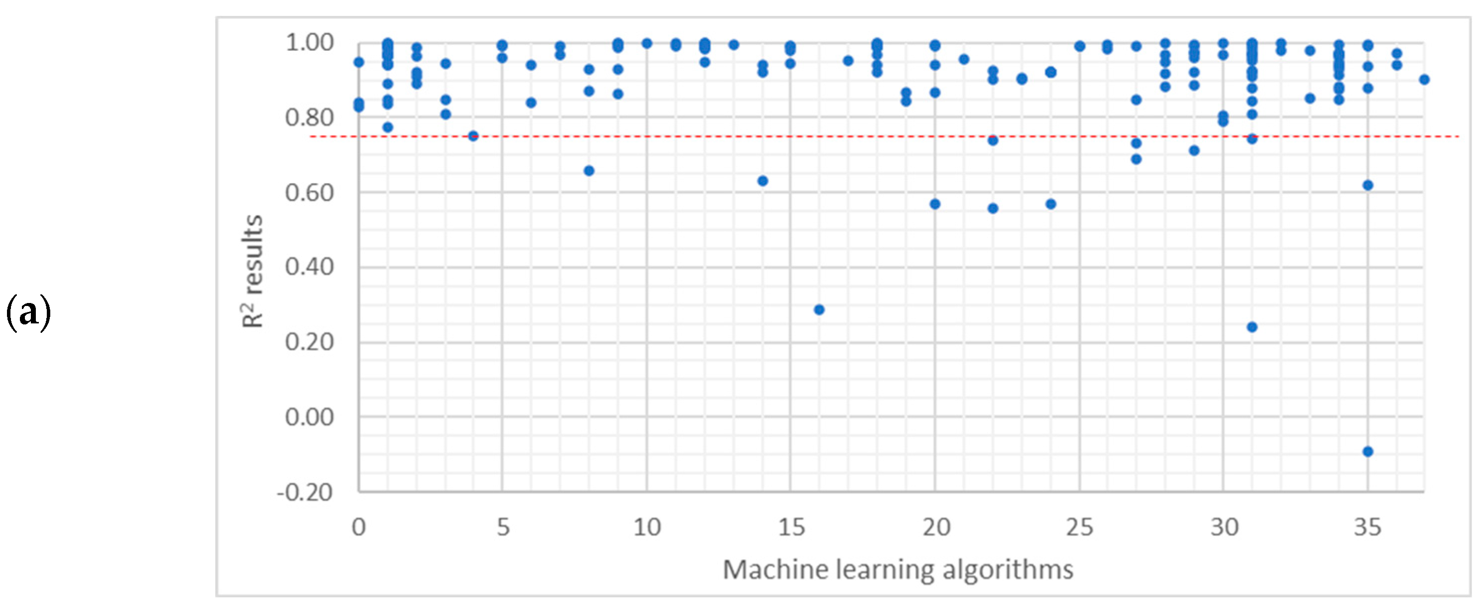
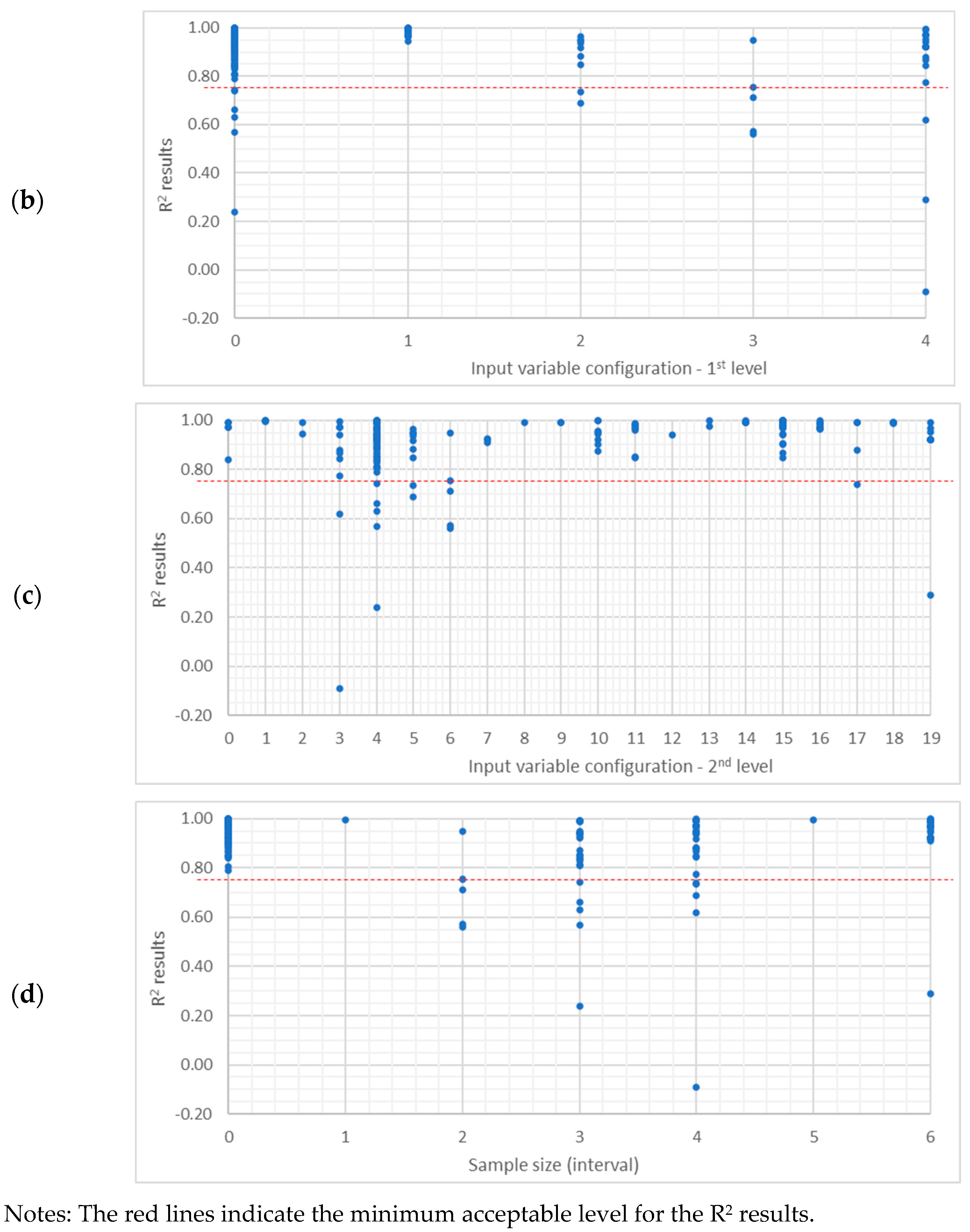
Appendix C. R2 Result Distributions Within Decision Subjects
| Decision Variable Heading | Items Under Headings | Value Assigned * | |
|---|---|---|---|
| Study aim | Studies with the aim of ‘improving the prediction performance by focusing on the dataset preparation stage’ | 0 | |
| Studies with the aims of ‘improving the prediction performance by focusing on the dataset preparation stage’ and ‘improving the prediction performance by focusing on issues related to the machine learning model preparation stage’ | 1 | ||
| Studies with the all aims determined in this study | 2 | ||
| Studies with the aims of ‘improving the prediction performance by focusing on the dataset preparation stage’ and ‘developing a particular model, approach, or framework’ | 3 | ||
| Studies with the aim of ‘improving the prediction performance by focusing on issues related to the machine learning model preparation stage’ | 4 | ||
| Studies with the aims of ‘improving the prediction performance by focusing on issues related to the machine learning model preparation stage’ and ‘developing a particular model, approach, or framework’ | 5 | ||
| Studies with the aim of ‘improving the prediction performance by focusing on issues related to the machine learning model preparation stage’ | 6 | ||
| Design stage | Early Design stage, Not Specified | ||
| Input variable configuration | 1st level ** | Building Climate +Building Surrounding effects+ Building Time + Building Time + Climate + Building | 0 1 2 3 4 |
| 2nd level ** | Building/Form/geometry+ Building/HVAC system+ Building/Internal gain+ Building/Orientation+ Building/Envelope | 0 | |
| Building/Form/geometry+Building/HVAC system+ Climate/Precipitation+ Climate/Pressure and moisture+ Climate/Temperature+ Climate/Wind+ Building/Internal gain+ Climate/Solar radiation and irradiation | 1 | ||
| Building/Form/geometry+ Building/Internal gain+ Building/Orientation+ Building/Envelope/+ Climate/Temperature | 2 | ||
| Building/Form/geometry+ Building/Orientation+ Building/Type+ Building/Envelope/+ Climate/Cloud+ Climate/Pressure and moisture+ Climate/Solar position related parameters+ Climate/Solar radiation and irradiation+ Climate/Temperature+ Climate/Wind+ Time | 3 | ||
| Building/Form/geometry+ Building/Orientation+ Building/Envelope/ | 4 | ||
| Building/Form/geometry+ Building/Orientation+ BuildingEnvelope/+ Surrounding effect/urban context morphology effect | 5 | ||
| Building/Form/geometry+ Building/Orientation+ Building/Envelope+ Time | 6 | ||
| Building/HVAC system+ Building/Envelope | 7 | ||
| Building/Internal gain+ Building/Envelope+ Climate/Solar position related parameters+ Climate/Solar radiation and irradiation | 8 | ||
| Building/Orientation+ Building/Envelope | 9 | ||
| Building/Envelope | 10 | ||
| Building/Envelope+ Building/Form/geometry+ Building/HVAC system | 11 | ||
| Building/Envelope+ Building/Form/geometry+ Building/HVAC system+ Building/Orientation+ Building/Internal gain+ Building/Type | 12 | ||
| Building/Envelope+ Building/Form/geometry+ Building/HVAC system+ Building/Orientation+ Climate/Precipitation+ Climate/Pressure and moisture+ Climate/Solar position related parameters+ Climate/Temperature+ Climate/Wind | 13 | ||
| Building/Envelope/+ Building/Form/geometry+ Building/HVAC system+ Climate/Pressure and moisture+ Climate/Temperature+ Building/Internal gain | 14 | ||
| Building/Envelope+ Building/Form/geometry+ Building/Orientation | 15 | ||
| Building/Envelope+ Building/Form/geometry+ Climate/Pressure and moisture+ Climate/Temperature+ Building/Internal gain+ Climate/Degree Days+ Climate/Solar radiation and irradiation | 16 | ||
| Building/Envelope+ Building/Orientation | 17 | ||
| Building/Envelope+ Building/Orientation+ Climate/Temperature Climate/Wind | 18 | ||
| Climate/Pressure and moisture+ Climate/Solar radiation and irradiation + Climate/Cloud+Climate/illuminance+ Room/Envelope+ Time | 19 | ||
| Sample size | Actual size | 54, 180, 201, 240, 768, 800, 1000, 1610, 2500, 3384, 4000, 5000, 5150, 5208, 5610, 6000, 10,000, 11,700, 25,000, 46,696, 421,245, 1,000,000, 1,001,000 | |
| As intervals | 0–1000 1000–2000 2000–3000 3000–4000 5000–6000 10,000 11,000 higher | 0 1 2 3 4 5 6 | |
| Output | Total energy consumption, Heating load, Cooling load, Visual comfort, Thermal comfort, Embodied energy/material stage impact, Environmental impact, Economy | ||
| Machine Learning Algorithm | Algorithm class | Component-based machine learning model, Decision Tree models, Gaussian Process regression, Genetic programming model, Lazy learning algorithm, Linear Regression, Minimax probability machine regression, Multivariate adaptive regression splines, Nearest Neighbors, Neural Networks, Support Vector Machine, Voting Heterogeneous Ensemble Learning | |
| Algorithm itself | Adaboost Artificial Neural Networks Back-propagation neural networks Bagging regressor Bayesian Regression Technique Classification and regression tree Component-based machine learning model Convolutional neural networks Decision Tree Deep neural networks Ensemble bagging trees Evolutionary multivariate adaptive regression splines Extreme Gradient Boosting Extreme Learning Machine Extremely randomized trees Gaussian process regression Generalized Linear Model Genetic programming model Gradient Boosting Decision Tree algorithm IBk Linear NN Search K-Nearest Neighbors Regressor Least square support vector machine Linear regression Locally Weighted Learning Long short-term memory model Minimax probability machine regression Model Trees Regression Multi-layer perceptron neural network Multiple linear regression Multivariate adaptive regression splines Radial basis function neural network Random forest algorithm Reduced Error Pruning Tree Stepwise linear regression Support vector machine Support vector regression Voting Heterogeneous Ensemble Learning Wavelet neural network | 0 1 2 3 4 5 6 7 8 9 10 11 12 13 14 15 16 17 18 19 20 21 22 23 24 25 26 27 28 29 30 31 32 33 34 35 36 37 | |
| Variables 1 | p-Value | Statistical Significance 2 | ||
|---|---|---|---|---|
| Between | Output | Machine learning algorithm | 8.76 × 10⁻¹ | Insignificant |
| categorical | Output | Machine learning algorithm class | 7.48 × 10⁻¹ | Insignificant |
| variables 3 | Sample size interval | Machine learning algorithm class | 1.67 × 10⁻² | Significant |
| Design stage targeted | Machine learning algorithm class | 3.37 × 10⁻³ | Significant | |
| Design stage targeted | 1st level input configuration | 1.08 × 10⁻³ | Significant | |
| 1st-level input configuration | Machine learning algorithm class | 1.93 × 10⁻⁴ | Significant | |
| 2nd-level input configuration | Machine learning algorithm class | 1.95 × 10⁻⁷ | Significant | |
| Study aim | Design stage targeted | 8.12 × 10⁻⁸ | Significant | |
| Sample size interval | Machine learning algorithm | 4.77 × 10⁻⁸ | Significant | |
| Design stage targeted | Machine learning algorithm | 4.94 × 10⁻⁹ | Significant | |
| Design stage targeted | Output | 1.57 × 10⁻⁹ | Significant | |
| 1st-level input configuration | Machine learning algorithm | 1.32 × 10⁻¹⁰ | Significant | |
| Study aim | Machine learning algorithm | 4.36 × 10⁻¹¹ | Significant | |
| Sample size interval | Output | 2.13 × 10⁻¹¹ | Significant | |
| Design stage targeted | 2nd level input configuration, | 1.31 × 10⁻¹³ | Significant | |
| Design stage targeted | Sample size-interval | 6.83 × 10⁻¹⁴ | Significant | |
| 2nd-level input configuration | Machine learning algorithm | 5.57 × 10⁻¹⁴ | Significant | |
| Study aim | Machine learning algorithm class | 5.92 × 10⁻¹⁶ | Significant | |
| 1st-level input configuration | Output | 4.92 × 10⁻¹⁷ | Significant | |
| Study aim | Output | 1.78 × 10⁻²⁹ | Significant | |
| Study aim | Sample size-interval | 5.78 × 10⁻³⁵ | Significant | |
| 2nd-level input configuration | Output | 6.57 × 10−56 | Significant | |
| 1st-level input configuration | Sample size-interval | 9.7 × 10−60 | Significant | |
| Study aim | 1st level input configuration | 2.01 × 10−60 | Significant | |
| 2nd-level input configuration, | Sample size-interval | 3.42 × 10−73 | Significant | |
| Study aim | 2nd level input configuration | 4.18 × 10−96 | Significant | |
| 1st-level input configuration | 2nd level input configuration | 1.40 × 10−105 | Significant | |
| Machine learning algorithm class | Machine learning algorithm | 1.27 × 10−204 | Significant | |
| Between | 2nd-level input configuration | Sample size | 0 | Insignificant |
| categorical | Machine learning algorithm class | Sample size | 8.80 × 10⁻¹ | Insignificant |
| and | Output | R2 results | 2.94 × 10⁻¹ | Insignificant |
| numerical | Machine learning algorithm class | R2 results | 1.84 × 10⁻¹ | Insignificant |
| variables 4 | Machine learning algorithm | Sample size | 1.22 × 10⁻² | Significant |
| Design stage targeted | Sample size | 1.21 × 10⁻² | Significant | |
| Design stage targeted | R2 results | 1.13 × 10⁻² | Significant | |
| 2nd-level input configuration | R2 results | 3.28 × 10⁻³ | Significant | |
| Machine learning algorithm | R2 results | 1.85 × 10⁻³ | Significant | |
| Study aim | R2 results | 6.94 × 10⁻⁴ | Significant | |
| Sample size interval | R2 results | 1.45 × 10⁻⁵ | Significant | |
| 1st-level input configuration | R2 results | 2.96 × 10⁻⁶ | Significant | |
| Study aim | Sample size | 4.08 × 10⁻¹⁰ | Significant | |
| 1st-level input configuration | Sample size | 4.08 × 10⁻¹⁰ | Significant | |
| Sample size interval | Sample size | 1.46 × 10⁻¹⁶ | Significant | |
| Output | Sample size | 6.41 × 10⁻²¹ | Significant | |
| Between numerical variables 4 | Sample size | R2 results | 8.2 × 10⁻⁵ | Significant |
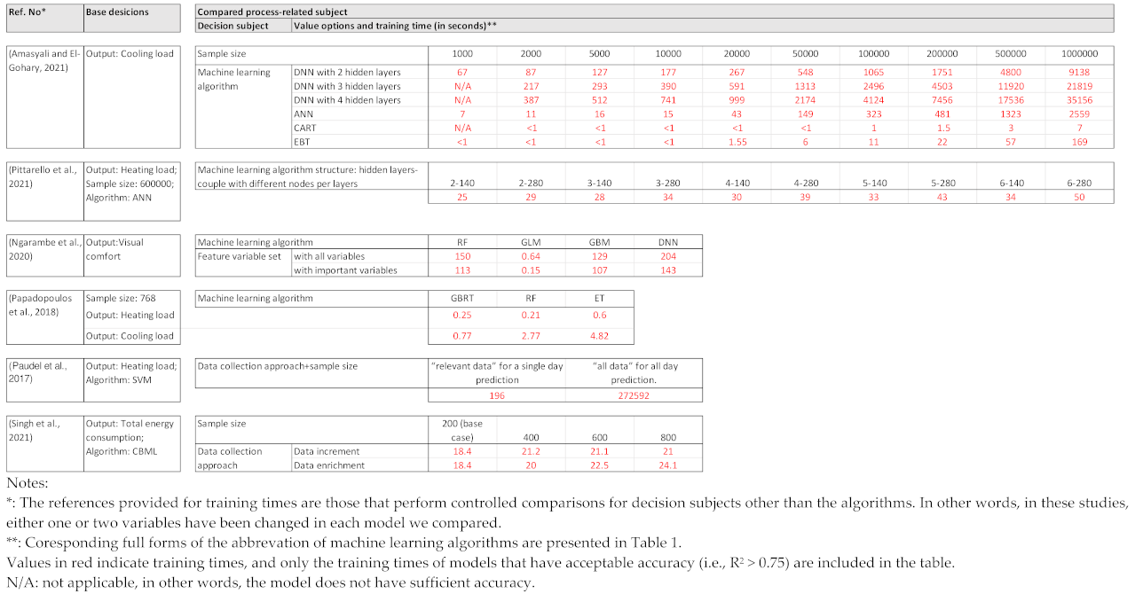
Appendix D. Training Times in the Studies That Comparatively Assessed Process-Related Variable Alternatives [8,29,35,51,67,71]
References
- Sadeghi, A.; Sinaki, R.Y.; Weckman, G.R.; Young, W.A. An intelligent model to predict energy performances of residential buildings based on deep neural networks. Energies 2020, 13, 571. [Google Scholar] [CrossRef]
- Geyer, P.; Singaravel, S. Component-based machine learning for performance prediction in building design. Appl. Energy 2018, 228, 1439–1453. [Google Scholar] [CrossRef]
- Clarke, J. Energy Simulation in Building Design, 2nd ed.; Routledge: London, UK, 2001. [Google Scholar] [CrossRef]
- Hensen, J.L.M.; Lamberts, R. (Eds.) Building Performance Simulation for Design and Operation, 2nd ed.; Routledge: London, UK, 2019. [Google Scholar] [CrossRef]
- Seyedzadeh, S.; Pour Rahimian, F.; Rastogi, P.; Glesk, I. Tuning machine learning models for prediction of building energy loads. Sustain. Cities Soc. 2019, 47, 101484. [Google Scholar] [CrossRef]
- Singh, M.M.; Singaravel, S.; Klein, R.; Geyer, P. Quick energy prediction and comparison of options at the early design stage. Adv. Eng. Inform. 2020, 46, 101185. [Google Scholar] [CrossRef]
- Flager, F.; Welle, B.; Bansal, P.; Soremekun, G.; Haymaker, J. Multidisciplinary process integration and design optimization of a classroom building. ITcon 2009, 14, 595–612. [Google Scholar]
- Pittarello, M.; Scarpa, M.; Ruggeri, A.G.; Gabrielli, L.; Schibuola, L. Artificial neural networks to optimize zero energy building (Zeb) projects from the early design stages. Appl. Sci. 2021, 11, 5377. [Google Scholar] [CrossRef]
- Barbaresi, A.; Ceccarelli, M.; Torreggiani, D.; Tassinari, P.; Bovo, M.; Menichetti, G. Application of Machine Learning Models for Fast and Accurate Predictions of Building Energy Need. Energies 2022, 15, 1266. [Google Scholar] [CrossRef]
- Sarker, I.H. Machine Learning: Algorithms, Real-World Applications and Research Directions. SN Comput. Sci. 2021, 2, 160. [Google Scholar] [CrossRef]
- Ahmad, T.; Chen, H.; Huang, R.; Yabin, G.; Wang, J.; Shair, J.; Azeem Akram, H.M.; Hassnain Mohsan, S.A.; Kazim, M. Supervised based machine learning models for short, medium and long-term energy prediction in distinct building environment. Energy 2018, 158, 17–32. [Google Scholar] [CrossRef]
- Lee, J.; Boubekri, M.; Liang, F. Impact of building design parameters on daylighting metrics using an analysis, prediction, and optimization approach based on statistical learning technique. Sustainability 2019, 11, 1474. [Google Scholar] [CrossRef]
- Fathi, S.; Srinivasan, R.; Fenner, A.; Fathi, S. Machine learning applications in urban building energy performance forecasting: A systematic review. Renew. Sustain. Energy Rev. 2020, 133, 110287. [Google Scholar] [CrossRef]
- Ahmad, T.; Chen, H.; Guo, Y.; Wang, J. A comprehensive overview on the data driven and large scale based approaches for forecasting of building energy demand: A review. Energy Build. 2018, 165, 301–320. [Google Scholar] [CrossRef]
- Amasyali, K.; El-Gohary, N.M. A review of data-driven building energy consumption prediction studies. Renew. Sustain. Energy Rev. 2018, 81, 1192–1205. [Google Scholar] [CrossRef]
- Dridi, J.; Bouguila, N.; Amayri, M. Transfer learning for estimating occupancy and recognizing activities in smart buildings. Build. Environ. 2022, 217, 109057. [Google Scholar] [CrossRef]
- Villa, S.; Sassanelli, C. The data-driven multi-step approach for dynamic estimation of buildings’ interior temperature. Energies 2020, 13, 6654. [Google Scholar] [CrossRef]
- de Wilde, P.; Martinez-Ortiz, C.; Pearson, D.; Beynon, I.; Beck, M.; Barlow, N. Building simulation approaches for the training of automated data analysis tools in building energy management. Adv. Eng. Inform. 2013, 27, 457–465. [Google Scholar] [CrossRef]
- Theil, H. Applied Economic Forecasting; by Henri Theil assisted by Beerens, G.A.C., De Leeuw, C.G., Tilanus, C.B.; Rand McNally: Chicago, IL, USA, 1966. [Google Scholar]
- Wang, C.; Yang, Y.; Causone, F.; Ferrando, M.; Ye, Y.; Gao, N.; Li, P.; Shi, X. Dynamic predictions for the composition and efficiency of heating, ventilation and air conditioning systems in urban building energy modeling. J. Build. Eng. 2024, 96, 110562. [Google Scholar] [CrossRef]
- Fu, T.; Tang, X.; Cai, Z.; Zuo, Y.; Tang, Y.; Zhao, X. Correlation research of phase angle variation and coating performance by means of Pearson’s correlation coefficient. Prog. Org. Coat. 2020, 139, 105459. [Google Scholar] [CrossRef]
- Laarne, P.; Zaidan, M.A.; Nieminen, T. ennemi: Non-linear correlation detection with mutual information. SoftwareX 2021, 14, 100686. [Google Scholar] [CrossRef]
- Zychlinski, S. Dython. 2024. Available online: http://shakedzy.xyz/dython/ (accessed on 17 January 2025).
- Buitinck, L.; Louppe, G.; Blondel, M.; Pedregosa, F.; Mueller, A.; Grisel, O.; Niculae, V.; Prettenhofer, P.; Gramfort, A.; Grobler, J.; et al. Scikit-Learn. 2013. Available online: https://scikit-learn.org/stable/index.html# (accessed on 17 January 2025).
- Risan, H.; Al-Azzawi, A.; Al-Zwainy, F. 4-T-, Chi-square, and F-distributions and hypothesis testing. In Statistical Analysis for Civil Engineers; Woodhead Publishing: Sawston, UK, 2025; pp. 155–214. ISBN 9780443273629. [Google Scholar] [CrossRef]
- Pinder, J. Chapter 9—Simulation fit significance: Chi-Square, A.N.O.V.A. Introduction to Business Analytics Using Simulation, 2nd ed.; Academic Press: Cambridge, MA, USA, 2022; pp. 273–325. ISBN 9780323917179. [Google Scholar] [CrossRef]
- Kottek, M.; Grieser, J.; Beck, C.; Rudolf, B.; Rubel, F. World Map of the Köppen-Geiger climate classification updated. Meteorol. Z. 2006, 15, 259–263. [Google Scholar] [CrossRef]
- Feng, K.; Lu, W.; Wang, Y. Assessing environmental performance in early building design stage: An integrated parametric design and machine learning method. Sustain. Cities Soc. 2019, 50, 101596. [Google Scholar] [CrossRef]
- Amasyali, K.; El-Gohary, N. Machine learning for occupant-behavior-sensitive cooling energy consumption prediction in office buildings. Renew. Sustain. Energy Rev. 2021, 142, 110714. [Google Scholar] [CrossRef]
- Li, X.; Yao, R. A machine-learning-based approach to predict residential annual space heating and cooling loads considering occupant behaviour. Energy 2020, 212, 118676. [Google Scholar] [CrossRef]
- Lin, Y.; Zhao, L.; Liu, X.; Yang, W.; Hao, X.; Tian, L.; Nord, N. Design optimization of a passive building with green roof through machine learning and group intelligent algorithm. Buildings 2021, 11, 192. [Google Scholar] [CrossRef]
- Yan, H.; Ji, G.; Yan, K. Data-driven prediction and optimization of residential building performance in Singapore considering the impact of climate change. Build. Environ. 2022, 226, 109735. [Google Scholar] [CrossRef]
- Jia, B.; Hou, D.; Wang, L.; Kamal, A.; Hassan, I.G. Developing machine-learning meta-models for high-rise residential district cooling in hot and humid climate. J. Build. Perform. Simul. 2022, 15, 553–573. [Google Scholar] [CrossRef]
- Martínez-Rocamora, A.; Rivera-Gómez, C.; Galán-Marín, C.; Marrero, M. Environmental benchmarking of building typologies through BIM-based combinatorial case studies. Autom. Constr. 2021, 132, 103980. [Google Scholar] [CrossRef]
- Ngarambe, J.; Yun, G.Y.; Kim, G.; Irakoze, A. Comparative performance of machine learning algorithms in the prediction of indoor daylight illuminances. Sustainability 2020, 12, 4471. [Google Scholar] [CrossRef]
- Sangireddy, S.A.R.; Bhatia, A.; Garg, V. Development of a surrogate model by extracting top characteristic feature vectors for building energy prediction. J. Build. Eng. 2019, 23, 38–52. [Google Scholar] [CrossRef]
- Tsay, Y.-S.; Yeh, C.-Y.; Chen, Y.-H.; Lu, M.-C.; Lin, Y.-C. A machine learning-based prediction model of lCCO2 for building envelope renovation in Taiwan. Sustainability 2021, 13, 8209. [Google Scholar] [CrossRef]
- Edwards, R.E.; New, J.; Parker, L.E.; Cui, B.; Dong, J. Constructing large scale surrogate models from big data and artificial intelligence. Appl. Energy 2017, 202, 685–699. [Google Scholar] [CrossRef]
- Sánchez, V.F.; Garrido Marijuan, A. Integrated model concept for district energy management optimisation platforms. Appl. Therm. Eng. 2021, 196, 117233. [Google Scholar] [CrossRef]
- Li, X.; Yao, R. Modelling heating and cooling energy demand for building stock using a hybrid approach. Energy Build. 2021, 235, 110740. [Google Scholar] [CrossRef]
- Todeschi, V.; Boghetti, R.; Kämpf, J.H.; Mutani, G. Evaluation of urban-scale building energy-use models and tools—Application for the city of Fribourg, Switzerland. Sustainability 2021, 13, 1595. [Google Scholar] [CrossRef]
- Tsanas, A.; Xifara, A. Accurate quantitative estimation of energy performance of residential buildings using statistical machine learning tools. Energy Build. 2012, 49, 560–567. [Google Scholar] [CrossRef]
- Naji, S.; Keivani, A.; Shamshirband, S.; Alengaram, U.J.; Jumaat, M.Z.; Mansor, Z.; Lee, M. Estimating building energy consumption using extreme learning machine method. Energy 2016, 97, 506–516. [Google Scholar] [CrossRef]
- Chen, R.; Tsay, Y.-S.; Zhang, T. A multi-objective optimization strategy for building carbon emission from the whole life cycle perspective. Energy 2023, 262, 125373. [Google Scholar] [CrossRef]
- Hey, J.; Siebers, P.-O.; Nathanail, P.; Ozcan, E.; Robinson, D. Surrogate optimization of energy retrofits in domestic building stocks using household carbon valuations. J. Build. Perform. Simul. 2023, 16, 16–37. [Google Scholar] [CrossRef]
- Singh, M.M.; Deb, C.; Geyer, P. Early-stage design support combining machine learning and building information modelling. Autom. Constr. 2022, 136, 104147. [Google Scholar] [CrossRef]
- Zhu, S.; Ma, C.; Zhang, Y.; Xiang, K. A hybrid metamodel-based method for quick energy prediction in the early design stage. J. Clean. Prod. 2021, 320, 128825. [Google Scholar] [CrossRef]
- Namlı, E.; Erdal, H.; Erdal, H.I. Artificial Intelligence-Based Prediction Models for Energy Performance of Residential Buildings; Springer International Publishing: Berlin/Heidelberg, Germany, 2019. [Google Scholar] [CrossRef]
- Moradzadeh, A.; Mansour-Saatloo, A.; Mohammadi-ivatloo, B.; Anvari-Moghaddam, A. Performance Evaluation of Two Machine Learning Techniques in Heating and Cooling Loads Forecasting of Residential Buildings. Appl. Sci. 2020, 10, 3829. [Google Scholar] [CrossRef]
- Sauer, J.; Mariani, V.C.; dos Santos Coelho, L.; Ribeiro MH, D.M.; Rampazzo, M. Extreme gradient boosting model based on improved Jaya optimizer applied to forecasting energy consumption in residential buildings. Evol. Syst. Interdiscip. J. Adv. Sci. Technol. 2022, 13, 577–588. [Google Scholar] [CrossRef]
- Papadopoulos, S.; Azar, E.; Woon, W.-L.; Kontokosta, C.E. Evaluation of tree-based ensemble learning algorithms for building energy performance estimation. J. Build. Perform. Simul. 2018, 11, 322–332. [Google Scholar] [CrossRef]
- Castelli, M.; Trujillo, L.; Vanneschi, L.; Popovič, A. Prediction of energy performance of residential buildings: A genetic programming approach. Energy Build. 2015, 102, 67–74. [Google Scholar] [CrossRef]
- Nebot, A.; Mugica, F. Energy performance forecasting of residential buildings using fuzzy approaches. Appl. Sci. 2020, 10, 720. [Google Scholar] [CrossRef]
- Roy, S.S.; Samui, P.; Nagtode, I.; Jain, H.; Shivaramakrishnan, V.; Mohammadi-ivatloo, B. Forecasting heating and cooling loads of buildings: A comparative performance analysis. J. Ambient Intell. Humaniz. Comput. 2020, 11, 1253–1264. [Google Scholar] [CrossRef]
- Moayedi, H.; Mosavi, A. Double-target based neural networks in predicting energy consumption in residential buildings. Energies 2021, 14, 1331. [Google Scholar] [CrossRef]
- Moayedi, H.; Mosavi, A. Suggesting a stochastic fractal search paradigm in combination with artificial neural network for early prediction of cooling load in residential buildings. Energies 2021, 14, 1649. [Google Scholar] [CrossRef]
- Navarro-Gonzalez, F.J.; Villacampa, Y. An octahedric regression model of energy efficiency on residential buildings. Appl. Sci. 2019, 9, 4978. [Google Scholar] [CrossRef]
- Zheng, S.; Lyu, Z.; Foong, L.K. Early prediction of cooling load in energy-efficient buildings through novel optimizer of shuffled complex evolution. Eng. Comput. 2020, 38, 105–119. [Google Scholar] [CrossRef]
- Almutairi, K.; Algarni, S.; Alqahtani, T.; Moayedi, H.; Mosavi, A. A TLBO-tuned neural processor for predicting heating load in residential buildings. Sustainability 2022, 14, 5924. [Google Scholar] [CrossRef]
- Cheng, M.-Y.; Cao, M.-T. Accurately predicting building energy performance using evolutionary multivariate adaptive regression splines. Appl. Soft Comput. 2014, 22, 178–188. [Google Scholar] [CrossRef]
- Han, Y.; Shen, L.; Sun, C. Developing a parametric morphable annual daylight prediction model with improved generalization capability for the early stages of office building design. Build. Environ. 2021, 200, 107932. [Google Scholar] [CrossRef]
- Ayoub, M. Contrasting accuracies of single and ensemble models for predicting solar and thermal performances of traditional vaulted roofs. Sol. Energy 2022, 236, 335–355. [Google Scholar] [CrossRef]
- Forouzandeh, N.; Zomorodian, Z.S.; Tahsildoost, M.; Shaghaghian, Z. Room energy demand and thermal comfort predictions in early stages of design based on the machine Learning methods. Intell. Build. Int. 2023, 15, 3–20. [Google Scholar] [CrossRef]
- Chen, R.; Tsay, Y.-S. Carbon emission and thermal comfort prediction model for an office building considering the contribution rate of design parameters. Energy Rep. 2022, 8, 8093–8107. [Google Scholar] [CrossRef]
- Wu, X.; Feng, Z.; Chen, H.; Qin, Y.; Zheng, S.; Wang, L.; Liu, Y.; Skibniewski, M.J. Intelligent optimization framework of near zero energy consumption building performance based on a hybrid machine learning algorithm. Renew. Sustain. Energy Rev. 2022, 167, 112703. [Google Scholar] [CrossRef]
- Hamida, A.; Alsudairi, A.; Alshaibani, K.; Alshamrani, O. Environmental impacts cost assessment model of residential building using an artificial neural network. Eng. Constr. Archit. Manag. 2021, 28, 3190–3215. [Google Scholar] [CrossRef]
- Singh, M.M.; Singaravel, S.; Geyer, P. Machine learning for early stage building energy prediction: Increment and enrichment. Appl. Energy 2021, 304, 117787. [Google Scholar] [CrossRef]
- Papinutto, M.; Boghetti, R.; Colombo, M.; Basurto, C.; Reutter, K.; Lalanne, D.; Kämpf, J.H.; Nembrini, J. Saving energy by maximising daylight and minimising the impact on occupants: An automatic lighting system approach. Energy Build. 2022, 268, 112176. [Google Scholar] [CrossRef]
- Abdou, N.; El Mghouchi, Y.; Jraida, K.; Hamdaoui, S.; Hajou, A.; Mouqallid, M. Prediction and optimization of heating and cooling loads for low energy buildings in Morocco: An application of hybrid machine learning methods. J. Build. Eng. 2022, 61, 105332. [Google Scholar] [CrossRef]
- Olinger, M.S.; de Araújo, G.M.; Dutra, M.L.; Silva, H.A.D.; Júnior, L.P.; de Macedo, D.D. Metamodel Development to Predict Thermal Loads for Single-family Residential Buildings. Mob. Netw. Appl. 2022, 27, 1977–1986. [Google Scholar] [CrossRef]
- Paudel, S.; Elmitri, M.; Couturier, S.; Nguyen, P.H.; Kamphuis, R.; Lacarrière, B.; Le Corre, O. A relevant data selection method for energy consumption prediction of low energy building based on support vector machine. Energy Build. 2017, 138, 240–256. [Google Scholar] [CrossRef]
- Singaravel, S.; Suykens, J.; Geyer, P. Deep convolutional learning for general early design stage prediction models. Adv. Eng. Inform. 2019, 42, 100982. [Google Scholar] [CrossRef]
- Chen, B.; Liu, Q.; Wang, L.; Deng, T.; Wu, X.; Chen, H.; Zhang, L. Multiobjective optimization of building energy consumption based on BIM-DB and LSSVM-NSGA-II. J. Clean. Prod. 2021, 294, 126153. [Google Scholar] [CrossRef]
- Chen, X.; Yang, H. A multi-stage optimization of passively designed high-rise residential buildings in multiple building operation scenarios. Appl. Energy 2017, 206, 541–557. [Google Scholar] [CrossRef]
- Sharif, S.A.; Hammad, A. Developing surrogate ANN for selecting near-optimal building energy renovation methods considering energy consumption, LCC and LCA. J. Build. Eng. 2019, 25, 100790. [Google Scholar] [CrossRef]
- ASHRAE. ASHRAE Guideline 14-2014 Measurement of Energy, Demand, and Water Savings. Atlanta: The American Society of Heating, Refrigerating and Air-Conditioning Engineers; ASHRAE: Peachtree Corners, GA, USA, 2014. [Google Scholar]
- Giannelos, S.; Bellizio, F.; Strbac, G.; Zhang, T. Machine learning approaches for predictions of CO2 emissions in the building sector. Electr. Power Syst. Res. 2024, 235, 110735. [Google Scholar] [CrossRef]
- Kazemi, F.; Asgarkhani, N.; Jankowski, R. Optimization-based stacked machine-learning method for seismic probability and risk assessment of reinforced concrete shear walls. Expert Syst. Appl. 2024, 255, 124897. [Google Scholar] [CrossRef]
- Sun, Y.; Haghighat, F.; Fung, B.C.M. The generalizability of pre-processing techniques on the accuracy and fairness of data-driven building models: A case study. Energy Build. 2022, 268, 112204. [Google Scholar] [CrossRef]
- Pessach, D.; Shmueli, E. Improving fairness of artificial intelligence algorithms in Privileged-Group Selection Bias data settings. Expert Syst. Appl. 2021, 185, 115667. [Google Scholar] [CrossRef]
- Ahmed, R.; Fahad, N.; Miah, M.S.U.; Hossen, M.J.; Mahmud, M.; Mostafizur Rahman, M.; Morol, M.K. A novel integrated logistic regression model enhanced with recursive feature elimination and explainable artificial intelligence for dementia prediction. Healthc. Anal. 2024, 6, 100362. [Google Scholar] [CrossRef]
- Kaushik, B.; Chadha, A.; Mahajan, A.; Ashok, M. A three layer stacked multimodel transfer learning approach for deep feature extraction from Chest Radiographic images for the classification of COVID-19. Eng. Appl. Artif. Intell. 2025, 147, 110241. [Google Scholar] [CrossRef]
- Sun, Y.; Haghighat, F.; Fung, B.C.M. A review of the -state-of-the-art in data -driven approaches for building energy prediction. Energy Build. 2020, 221, 110022. [Google Scholar] [CrossRef]
- Sina, A.; Abdolalizadeh, L.; Mako, C.; Torok, B.; Amir, M. Systematic review of deep learning and machine learning for building energy. Front. Energy Res. 2022, 10, 786027. [Google Scholar] [CrossRef]
- Ahmad, T.; Zhang, H.; Yan, B. A review on renewable energy and electricity requirement forecasting models for smart grid and buildings. Sustain. Cities Soc. 2020, 55, 102052. [Google Scholar] [CrossRef]


| Number of Studies * | |||||
|---|---|---|---|---|---|
| Algorithm Type | Algorithm Class | Algorithms | Abbreviation | All Studies | Studies for Early Design Stage |
| Ensemble | Bagging Algorithm | Bootstrap Aggregating–Bagging Algorithm | BA | 1 | |
| Decision Tree | Adaboost | AB | 2 | 1 | |
| Bagging Regressor | BR | 1 | 1 | ||
| Ensemble Bagging Trees | EBT | 1 | |||
| Extra Tree Algorithm | ET | 1 | |||
| Extreme Gradient Boosting | XGBoost | 6 | |||
| Extremely Randomized Trees | ERT | 2 | 1 | ||
| Gradient Boosting Decision Tree Algorithm | GBRT | 9 | 1 | ||
| Random Forest | RF | 14 | 3 | ||
| Light Gradient Boosting Machine Model | Light Gradient Boosting Machine Model | LGBM | 1 | ||
| Voting Heterogeneous Ensemble Learning | Voting Heterogeneous Ensemble Learning | ELVoting | 1 | ||
| Single | Component-based Machine Learning | Component-based Machine Learning | CBML | 2 | 2 |
| Decision Tree | Classification and Regression Tree | CART | 2 | ||
| Decision Tree | DT | 3 | 2 | ||
| Model Trees Regression | M5P | 1 | |||
| Reduced Error Pruning Tree | REPTree | 1 | |||
| Design and Analysis of Computer Experiments | Design and Analysis of Computer Experiments | DACE | 1 | 1 | |
| Fuzzy Logic | Adaptive Neuro Fuzzy Inference System | ANFIS | 1 | ||
| Fuzzy Inductive Reasoning | FIR | 1 | |||
| Gaussian Process Regression | Gaussian Process Regression | GPR | 3 | 1 | |
| Generalized Additive Models | Generalized Additive Models | GAM | 1 | ||
| Genetic Programming | Genetic Programming | GP | 2 | ||
| Lazy Learning Algorithm | IBk Linear Nearest Neighbour Search | Ibk | 1 | ||
| Locally Weighted Learning | LWL | 1 | |||
| Linear Regression | Bayesian Regression Technique | 1 | |||
| Bayesian Ridge Regression | 1 | 1 | |||
| Elastic Net | EN | 1 | |||
| Generalized Linear Model | GLM | 1 | 1 | ||
| Huber | 1 | 1 | |||
| Iteratively Reweighted Least Squares | IRLS | 1 | |||
| Least Absolute Shrinkage and Selection Operator | LASSO | 3 | 1 | ||
| Linear Regression | LR | 7 | 1 | ||
| Multiple Linear Regression | MLR | 2 | |||
| Multivariate Adaptive Regression Splines | MARS | 3 | 1 | ||
| Ordinary Least-Squares Linear Regression | OLS | 1 | |||
| Random Sample Consensus | RANSAC | 1 | 1 | ||
| Ridge Regression | RR | 2 | 1 | ||
| Stepwise Linear Regression | SLR | 2 | |||
| Theil Sen | Theil Sen | 1 | 1 | ||
| Minimax Probability Machine Regression | Minimax Probability Machine Regression | MPMR | 1 | ||
| Multivariate Adaptive Regression Splines | Evolutionary Multivariate Adaptive Regression Splines | EMARS | 1 | ||
| Nearest Neighbors | K-Nearest Neighbors Regressor | KNN | 4 | 2 | |
| Neural Networks | Artificial Neural Networks | ANN | 24 | 7 | |
| Back-Propagation Neural Networks | BPNN | 3 | |||
| Convolutional Neural Networks | CNN | 2 | 2 | ||
| Deep Neural Networks | DNN | 4 | 1 | ||
| Extreme Learning Machine | ELM | 2 | 1 | ||
| Feed Forward Neural Networks | 1 | ||||
| Long Short-term Memory Model | LSTM | 2 | 1 | ||
| Multi-layer Perceptron Neural Network | MLP | 7 | |||
| Radial Basis Function Neural Network | RBFNN | 2 | |||
| Wavelet Neural Networks | WNN | 1 | |||
| Octahedric Regression Model | Octahedric Regression Model | 1 | |||
| Support Vector Machine | LeastSquare Support Vector Machine | LSSVM | 1 | ||
| Support Vector Machine | SVM | 9 | 1 | ||
| Support Vector Regression | SVR | 10 | 1 | ||
Disclaimer/Publisher’s Note: The statements, opinions and data contained in all publications are solely those of the individual author(s) and contributor(s) and not of MDPI and/or the editor(s). MDPI and/or the editor(s) disclaim responsibility for any injury to people or property resulting from any ideas, methods, instructions or products referred to in the content. |
© 2025 by the authors. Licensee MDPI, Basel, Switzerland. This article is an open access article distributed under the terms and conditions of the Creative Commons Attribution (CC BY) license (https://creativecommons.org/licenses/by/4.0/).
Share and Cite
Kömürcü, D.; Edis, E. Machine Learning Modeling for Building Energy Performance Prediction Based on Simulation Data: A Systematic Review of the Processes, Performances, and Correlation of Process-Related Variables. Buildings 2025, 15, 1301. https://doi.org/10.3390/buildings15081301
Kömürcü D, Edis E. Machine Learning Modeling for Building Energy Performance Prediction Based on Simulation Data: A Systematic Review of the Processes, Performances, and Correlation of Process-Related Variables. Buildings. 2025; 15(8):1301. https://doi.org/10.3390/buildings15081301
Chicago/Turabian StyleKömürcü, Damla, and Ecem Edis. 2025. "Machine Learning Modeling for Building Energy Performance Prediction Based on Simulation Data: A Systematic Review of the Processes, Performances, and Correlation of Process-Related Variables" Buildings 15, no. 8: 1301. https://doi.org/10.3390/buildings15081301
APA StyleKömürcü, D., & Edis, E. (2025). Machine Learning Modeling for Building Energy Performance Prediction Based on Simulation Data: A Systematic Review of the Processes, Performances, and Correlation of Process-Related Variables. Buildings, 15(8), 1301. https://doi.org/10.3390/buildings15081301