Article

Investigating the Effects of 2D/3D Urban Morphology on Land Surface Temperature Using High-Resolution Remote Sensing Data

1
China Aero Geophysical Survey and Remote Sensing Center for Natural Resources, Beijing 100083, China
2
Key Laboratory of Airborne Geophysics and Remote Sensing Geology, Ministry of Natural Resources of the People’s Republic of China, Beijing 100083, China
3
Technology Innovation Center for Geohazards Identification and Monitoring with Earth Observation System, Ministry of Natural Resources of the People’s Republic of China, Beijing 100083, China
4
Surveying and Mapping Institute Lands and Resource Department of Guangdong Province, Guangzhou 510663, China
5
Key Laboratory of 3D Information Acquisition and Application, Ministry of Education of the People’s Republic of China, Capital Normal University, Beijing 100048, China
*
Author to whom correspondence should be addressed.
Buildings 2025, 15(8), 1256; https://doi.org/10.3390/buildings15081256
Submission received: 24 February 2025 / Revised: 30 March 2025 / Accepted: 8 April 2025 / Published: 10 April 2025
(This article belongs to the Special Issue Advanced Studies in Urban and Regional Planning—2nd Edition)

Abstract

:
Understanding the influence of urban morphology on Land Surface Temperature (LST) is essential for urban planning, development, and mitigating the urban heat island effect. Leveraging high-resolution remote sensing data, this study systematically extracted 64 2D urban morphological parameters (UMPs) and 28 3D UMPs, along with their corresponding summer and winter LST data, at both the grid level (using a 30 m × 30 m grid as the minimum unit) and the block level (using an urban block as the minimum unit). The 2D UMPs were derived from landscape indices of land cover, while the 3D UMPs included 3D building-related UMPs (BUMPs) and tree-related UMPs (TUMPs). Ultimately, multiple statistical methods were employed to investigate the complex mechanisms through which these 2D and 3D UMPs influence LST across summer and winter. This study showed the following results: (1) Most 2D and 3D UMPs significantly correlated with LST in both seasons at the grid/block levels, with stronger correlations at block level. (2) Stepwise regression revealed that combining 2D and 3D UMPs enhanced LST explanation, achieving R2 = 70.9% (summer) and 65.7% (winter) for the entire area, with consistent results in built-up zones. (3) Relative importance analysis identified 35 (summer) and 28 (winter) influential features, which were ranked as follows: 2D UMPs > 3D BUMPs > 3D TUMPs. This highlights 2D UMPs’ dominance while confirming 3D UMPs’ significance. These findings emphasize the need for integrated 2D and 3D urban design, considering both planar layouts and vertical configurations of buildings/vegetation. This study provides practical guidance for thermal environment mitigation and sustainable urban development through optimized spatial planning.

1. Introduction

With the rapid advancement of global economic and social development, urbanization has emerged as an irreversible worldwide phenomenon, representing one of the most profound aspects of global transformation [1,2,3]. The proliferation of artificial structures in urban areas has substantially modified the thermal properties of underlying surfaces. Concurrently, the exponential growth of urban populations has intensified production, transportation, and consumption activities, leading to the emission of considerable amounts of heat and greenhouse gases. These factors collectively contribute to a range of urban thermal environmental challenges, most prominently the urban heat island (UHI) effect [4]. The UHI effect is associated with extreme weather phenomena, including elevated temperatures and intense precipitation events, while also exacerbating energy consumption, environmental pollution, and negative impacts on public health and quality of life [5,6,7,8,9].
Land Surface Temperature (LST) serves as the most direct indicator of the UHI effect [10], playing a crucial role in regulating near-surface atmospheric temperatures and significantly influencing urban residents’ thermal comfort [7]. Urban morphology, which describes the spatial configuration and distribution of urban elements, is shaped by the complex interplay of natural, social, and economic factors within urban spaces [11,12]. Substantial evidence demonstrates that urban morphology exerts a significant influence on the urban thermal environment [13,14]. Consequently, understanding the spatial distribution patterns of urban LST and optimizing urban spatial configurations through comprehensive analysis of urban morphology’s impact on LST represents a strategic approach to mitigating UHI effects and related thermal environmental issues. This methodology carries substantial implications for urban planning and sustainable urban management [15].
Traditional thermal environment studies primarily rely on meteorological station data, but their sparse distribution results in a limited resolution and uneven temperature measurements that fail to capture urban thermal patterns comprehensively [14]. Remote sensing has revolutionized this field by enabling spatially continuous LST monitoring while simultaneously acquiring urban morphology data (land use/cover, landscape patterns, settlement density) [16,17]. While moderate-resolution sensors (e.g., Landsat, MODIS) are widely used for UHI studies [18,19], Landsat 8’s Thermal Infrared Sensor (TIRS), featuring two spectral bands (100 m native resolution), provides resampled 30 m thermal data through systematic processing. This sensor offers unique capabilities for LST estimation, combining the enhanced 30 m spatial resolution, systematic global coverage, and free data accessibility—characteristics particularly valuable for UHI studies [10,20].
However, even Landsat’s improved resolution remains insufficient for detailed urban morphology analysis, necessitating integration with higher-resolution data. Zhou et al. [21] combined Landsat LST data with multiresolution land use data (0.6 m/30 m) and the normalized vegetation index, finding enhanced LST prediction with a higher categorical resolution of land use. Berger et al. [15] integrated IKONOS-2 multispectral imagery with airborne UltraCamX data and RIEGL Light Detection and Ranging (LiDAR)-derived height information to perform detailed land use classification. At the block level, they extracted 13 two-dimensional (2D) features (e.g., building, grass, and tree coverage) and 13 13 three-dimensional (3D) features (e.g., building/tree height, volume, and Sky View Factor (SVF)). Using multi-seasonal Landsat LST data, they systematically analyzed spatiotemporal relationships between these 2D/3D features and LST across different regions. However, these studies have established bivariate relationships between urban 2D/3D features and LST, but their explanatory power remains limited by two key gaps: Oversimplified analysis: Most approaches examine morphological parameters in isolation, neglecting their synergistic effects on thermal patterns. Incomplete urban representation: Current frameworks focus primarily on physical attributes (surface cover/geometry) while largely ignoring functional dimensions—particularly Urban Functional Zones (UFZs) that integrate land cover with socioeconomic activities [22]. Recent studies have demonstrated that UFZs significantly influence LST. For instance, Huang et al. [14] conducted land cover and UFZ classification using ZY-3 imagery and geographic information data, extracting both 2D (land cover types) and 3D (building morphology) features to analyze the impact of UFZ 2D/3D morphology on LST across multiple LST scenes. Yu et al. [23] utilized ZY-3 imagery to generate a land cover map and Digital Surface Models (DSMs) from stereopairs, quantifying block-level relationships between landscape configuration (2D/3D) and LST. Despite utilizing high-resolution remote sensing imagery and incorporating UFZs in their analyses, these studies exhibit two critical methodological constraints related to 3D data acquisition: (1) temporal discrepancies between 3D height data (sourced from geographic information data) and 2D image capture, compounded by registration inaccuracies during data fusion, and (2) inherent limitations of stereopair-derived DSMs in distinguishing true object height from underlying terrain elevation.
Furthermore, we observed that most existing studies have focused on megacities such as Beijing, Shanghai, Guangzhou, Wuhan, and Nanjing [14,23,24,25], while research on small and medium-sized cities (SMSCs) remains relatively limited. According to the National Bureau of Statistics of China, SMSCs are defined as urban areas with a central urban population ranging from several hundred thousand to one million [26]. Notably, there is insufficient exploration of the effects of 2D/3D UMPs on LST in SMSCs.
Based on the preceding analysis, we identify several research gaps in the effects of urban morphology on LST: (1) a paucity of studies focusing on SMSCs; (2) data limitations in temporal coverage and inadequate spatial resolution of imagery and 3D information, which hinder accurate characterization of refined 2D/3D urban morphology; and (3) insufficient investigation into the integrated effects of urban morphology and human activities on LST patterns. To address these gaps, our study took Ziyang City, Sichuan Province, as an example of an SMSC and explored the impact of 2D and 3D urban morphological parameters (UMPs) on LST using high-resolution remote sensing data. Firstly, we obtained high-precision distribution of land covers and UFZs based on airborne LiDAR point clouds, aerial images, and open geographic information data. Secondly, we extracted refined 2D and 3D UMPs and their corresponding summer and winter LST from Landsat 8 images at both the grid level and block level. Finally, we used statistical analysis methods to investigate the effects of 2D and 3D UMPs on the LST in summer and winter seasons at the grid level and block level. The study results provide invaluable guidance for mitigating the UHI effect in SMSCs, facilitating rational urban planning, and ensuring the efficient utilization of resources.

2. Methods

2.1. Overview of the Methodology

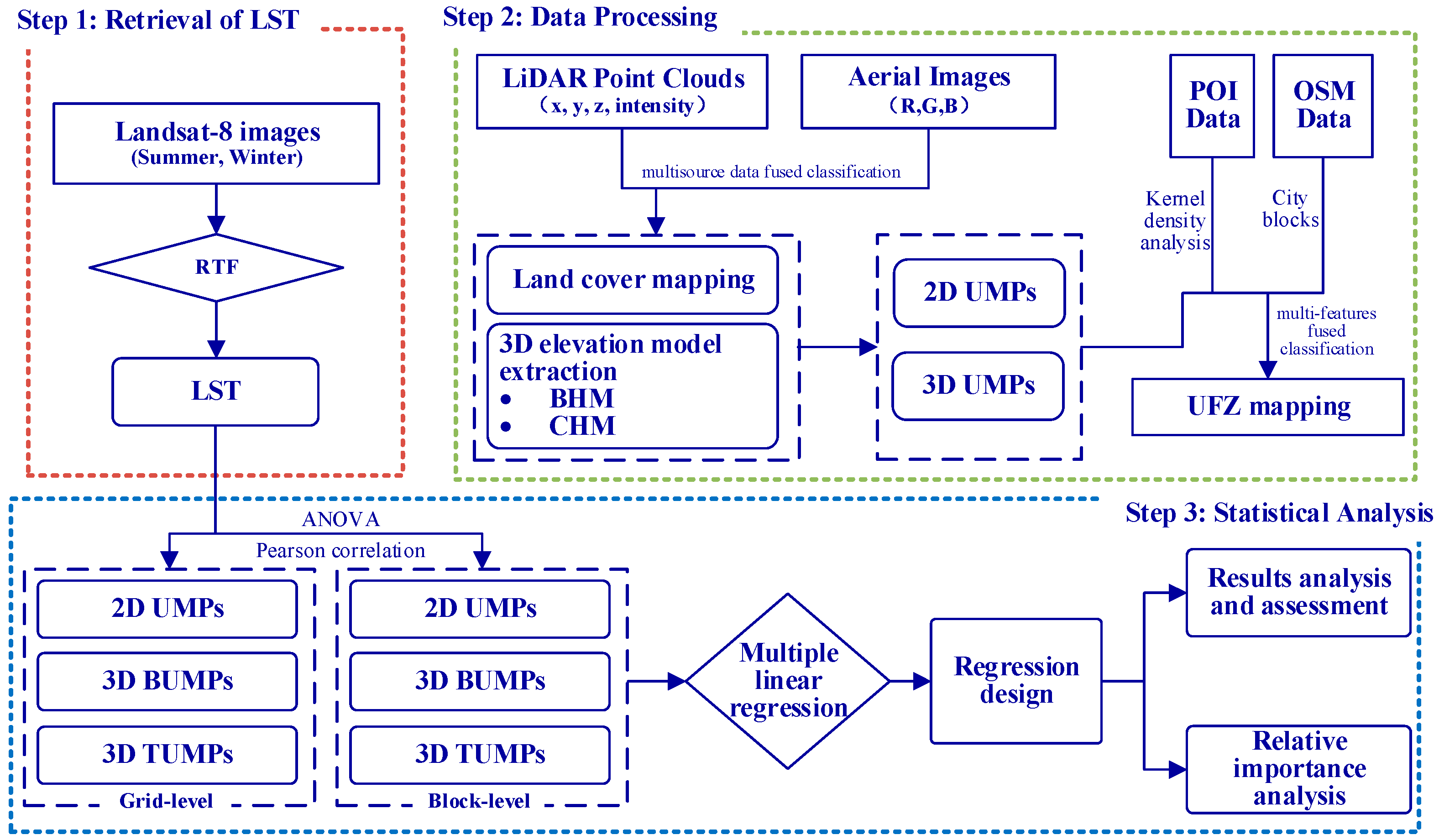
The workflow for studying the effects of 2D and 3D UMPs on LST at the grid level and block level using high-resolution remote sensing data is illustrated in Figure 1. It mainly consists of three steps: (1) Retrieval of LST: We retrieved LST using the radiative transfer equation method for both summer and winter seasons. (2) Land cover and UFZ classification: First, we fused airborne LiDAR and aerial images for land cover classification, extracting both the Building Height Model (BHM) and the Canopy Height Model (CHM). Then, UFZs were classified by integrating 2D and 3D UMPs with POI kernel density features. (3) Statistical analysis: We extracted 2D and 3D UMPs at both the grid level and block level. Various statistical methods were then employed to analyze the impact of these UMPs on LST during summer and winter, followed by a detailed evaluation of the results.

2.2. Study Area and Data Sources

2.2.1. Study Area

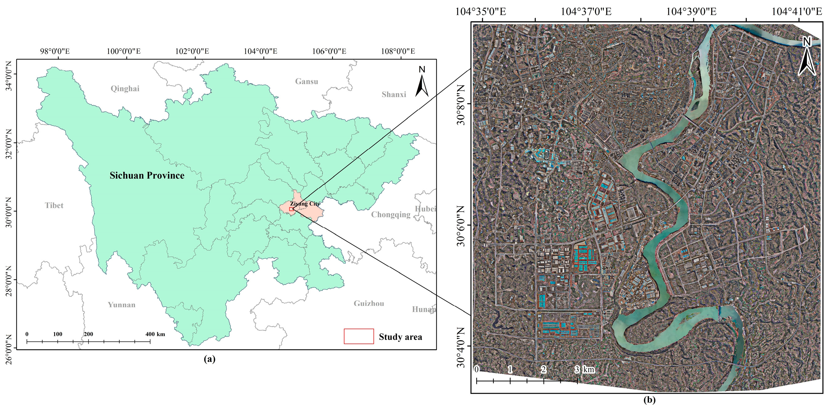
The study area is located in Ziyang City, Sichuan Province, China, as shown in Figure 2. Ziyang is situated in the central part of the Sichuan Basin, with geographic coordinates ranging from 104°21′ to 105°27′ E and 29°15′ to 30°17′ N. Positioned between the major cities of Chengdu and Chongqing, Ziyang is the only city in Sichuan Province that connects these two urban centers. This unique position makes it a crucial regional hub and a prime example of a rapidly developing SMSC. Ziyang City experiences a subtropical monsoon climate, with average temperatures around 26.5 °C in summer and 6.5 °C in winter. August is the hottest month, while January is the coldest. The Tuojiang River is the primary water source in the study area, which features a topography that descends from west to east. The main landforms are hilly terrain and fluvial/alluvial plains, characterized by a simple landscape structure and relatively flat strata. The study area covers approximately 115 km2, including the urban and parts of suburbs. The land cover is diverse, comprising both man-made and natural landscapes such as buildings, roads, vegetation, croplands, bare land, and water.

2.2.2. Data Sources

The primary data sources utilized in this study comprise airborne LiDAR point clouds, aerial imagery, Landsat 8 satellite imagery, Point of Interest (POI) data, and OpenStreetMap (OSM) road network data. It should be noted that the acquisition of Land Surface Temperature (LST) data imposes stringent requirements on Landsat 8 imagery regarding acquisition timing and cloud cover conditions, while POI and OSM data often suffer from update delays. To ensure temporal consistency across datasets as much as possible, we adopted the acquisition date of the airborne LiDAR point clouds and aerial imagery (9 September 2017) as our temporal reference. Considering that artificial structures typically exhibit minimal changes over short periods, we restricted the temporal coverage of all other data sources to the period between 2017 and 2019. The detailed descriptions of all the data sources employed in this study are systematically presented in Table 1.
(1) LiDAR Point Clouds and Aerial Images
The LiDAR point clouds and aerial images were synchronously acquired using an Airborne Laser Scanning (ALS) system on 9 September 2017. This ALS system is equipped with a RIEGL VUX-1LR LiDAR scanner (Riegl Laser Measurement Systems GmbH, Horn, Austria), a PHASE ONE IXU1000-R high-resolution digital camera (Phase One A/S, Copenhagen, Denmark), and a POS system. In this study, the average point cloud density is 20 points per square meter (pts/m2), with a horizontal resolution of 0.17 m and a vertical resolution of 0.2 m. The recorded elevations range from a minimum of 338 m to a maximum of 519.19 m. The attributes of the point clouds include X, Y, and Z coordinates and intensity information. These point clouds were utilized for land cover classification and the extraction of 2D and 3D UMPs.
Each original aerial image measures 11,608 × 8708 pixels with a resolution of 3.33 mm. These aerial images, which include red, green, and blue spectral bands, underwent preprocessing in Pix4Dmapper (Pix4D SA, Prilly, Switzerland), including orthorectification and mosaicking. The final orthorectified aerial images used in our study were set to a resolution of 1 m. These images were utilized for land cover classification, extraction of urban 2D and 3D UMPs, and block delineation.
(2) Landsat 8 Remote Sensing Images
Landsat 8 images were acquired from the USGS official website (URL: https://earthexplorer.usgs.gov/, accessed on 1 March 2023) and utilized for retrieving LST. These images include nine Operational Land Imager (OLI) bands and two TIRS bands. We selected Landsat 8 images spanning from January 2017 to December 2019, corresponding to the time of airborne LiDAR and aerial images acquisition. Ultimately, only three images satisfied the cloud-free requirement for our study, comprising one from the summer season and two from the winter season.
(3) POI Data
POI data exemplify the rapid advancement of internet technology and the continuous updates to electronic maps. They integrate daily human movements with geographical information, offering robust computational and expressive capabilities. These data are instrumental for extracting geographical spatial information and conducting population analyses based on specific locations [27,28]. POI data encompass various attributes such as name, address, coordinates, and category within internet-based electronic maps. For this study, POI data were sourced from the Amap Open Platform (URL: https://lbs.amap.com/, accessed on 1 May 2023) using interfaces provided by Amap, with Python 3.7 utilized to crawl POI data across the study area. Following data refinement, a total of 36,216 vector points were acquired. POI data played a crucial role in classifying UFZs in this research.
(4) OSM Road Network Data
OSM is a free, open-source, and editable map database created and maintained by volunteers worldwide. OSM provides extensive global coverage and rich geographical data, including streets, buildings, rivers, lakes, mountains, and public facilities. It is widely used in urban planning, 3D modeling, and neighborhood boundary delineation [29,30,31,32]. In this study, road network data for the study area were obtained from the OSM official website (URL: https://www.openstreetmap.org/, accessed on 20 May 2023). We selected major urban roads, secondary urban roads, urban branch roads, urban elevated and express roads, and railways as the basis for neighborhood delineation. OSM data provided detailed road network distribution information within the study area, facilitating the subdivision of blocks.

2.3. Retrieval of LST

In this study, we employed the radiative transfer equation (RTF) method for retrieving LST. The basic principle is as follows: first, estimate the impact of the atmosphere on surface thermal radiation; second, calculate the intensity of surface thermal radiation by subtracting the atmospheric influence from the total thermal radiation observed by the satellite sensor; and finally, convert the thermal radiation intensity into the corresponding LST. The radiative transfer equation for LST retrieval is as follows [33,34]:
L λ = ε B T s + 1 ε L τ + L ,
where L λ represents the TIRS radiance received by the satellite sensor.   ε represents the surface emissivity;   B T s denotes the radiance of a blackbody in TIRS band; T s is the true LST; τ stands for the transmittance of the atmosphere in the TIRS; L denotes the atmospheric upwelling radiance; L represents the atmospheric downwelling radiance. The parameters τ , L , and L can be obtained by querying the imaging time, central latitude, and longitude of Landsat 8 images on relevant websites provided by NASA (URL: http://atmcorr.gsfc.nasa.gov/, accessed on 10 March 2023).
The formula for calculating the radiance B T s of a blackbody in the TIRS band is as follows:
B T s = L λ L τ 1 ε L τ ε ,
Next, under the assumption that the earth’s surface behaves as a blackbody, B T s is converted to brightness temperature T B as measured by the satellite sensor. The formula is as follows:
T B = K 2 ln K 1 B T s + 1 ,
where K 1 = 774.89   W / m 2 s r μ m and K 2 = 1321.08   K for TIRS band 10.
Finally, by correcting for the surface emissivity, the LST T s is calculated as follows:
T s = T B 1 + λ T B ρ ln ε ,
where λ is the wavelength of emitted radiation (for TIRS band 10, λ = 10.9   μ m ), and ρ = 1.438 × 10 2   m K .
The surface emissivity ε is estimated as follows, based on the research conducted by Dash et al. (2010) and Xie et al. (2012) [35,36]:
ε = 1.0094 + 0.047 ln N D V I ,
where N D V I is the Normalized Difference Vegetation Index, and its calculation formula is as follows [37]:
N D V I = N I R R N I R + R ,
where N I R represents the near-infrared band, and R represents the red band.
In this study, we utilized ENVI 5.3 software to conduct radiometric calibration and atmospheric correction on Landsat 8 images and subsequently retrieved the LST using the RTF method. Table 2 presents the basic information of the three images, along with the atmospheric profile parameters provided by NASA. Notably, the TIRS bands were resampled to a 30 m resolution through the cubic convolution algorithm, as implemented by the U.S. Geological Survey [38]. Finally, we acquired three LST images at a 30 m resolution. Specifically, we averaged the two winter LST images.

2.4. Land Cover and UFZ Mapping

2.4.1. Land Cover Mapping

Accurate land cover classification is crucial for extracting detailed 2D and 3D UMPs. Numerous studies have shown that the fusion of multisource remote sensing data effectively leverages the complementary advantages of different features, significantly improving the accuracy of land cover classification [39,40]. Based on aerial images, Google Maps, and on-site surveys, the land cover in the study area was categorized into building land, bare soil, cropland, grassland, road, woodland, and water.
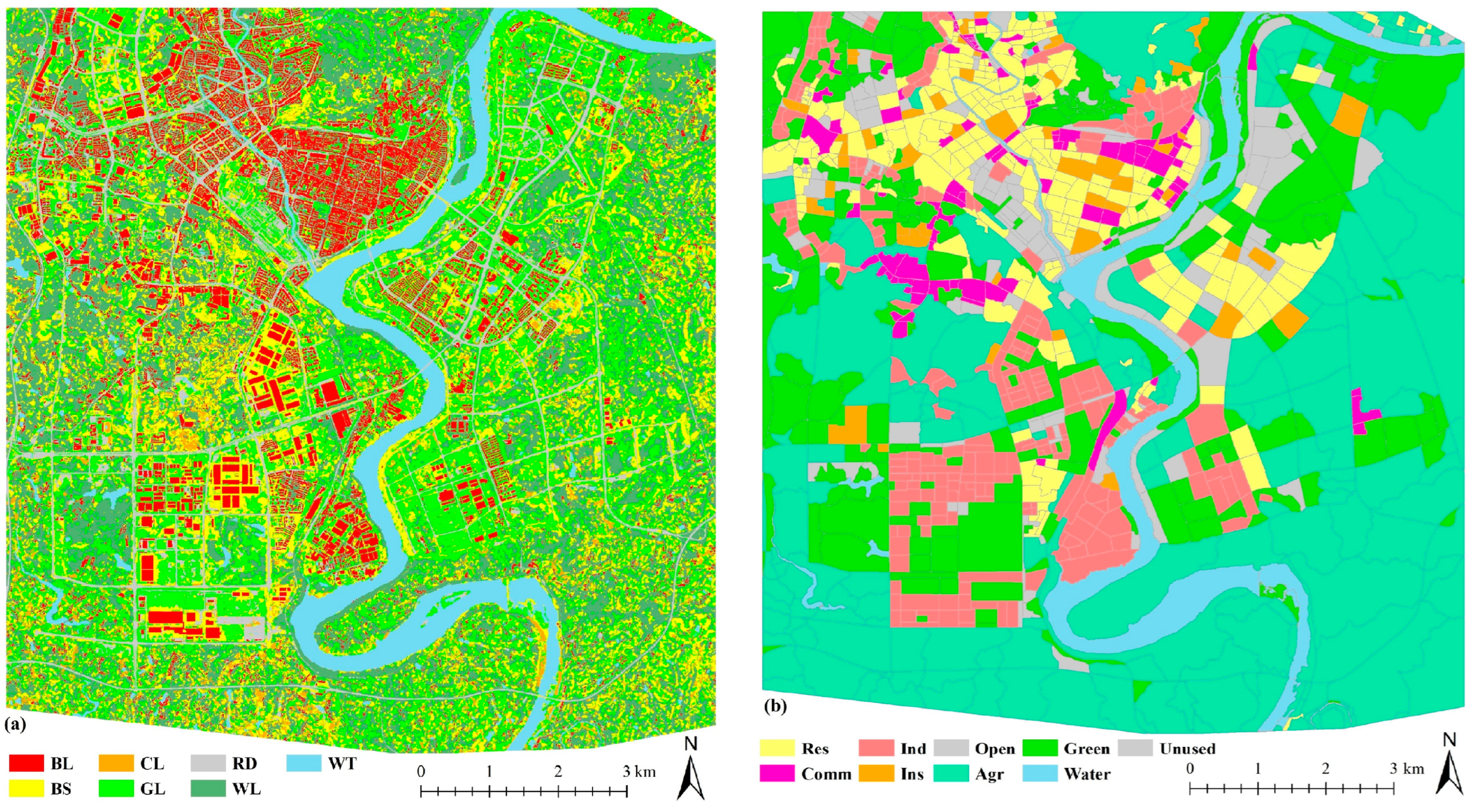
We employed an object-oriented land cover classification by integrating airborne LiDAR and aerial images. The classification process involved four main steps: (1) Feature extraction: We extracted the normalized Digital Surface Model (nDSM), intensity model, roughness model, and texture features based on the nDSM, including variance, homogeneity, contrast, dissimilarity, entropy, second moment, and correlation. Additionally, we extracted the red, green, and blue bands, along with the visible light vegetation index, from the aerial images. (2) Multiresolution segmentation: We conducted multiresolution segmentation based on aerial images and nDSM. (3) Sample selection: We referenced high-resolution Google Earth images and aerial images to label the training and validation samples. (4) Multiple features fusion and supervised classification: We ultimately selected the classification scheme with the highest accuracy, incorporating all features, for producing the land cover mapping results. This scheme achieved an overall accuracy of 94.61% and a kappa coefficient of 0.93, with user accuracy and producer accuracy for all land cover classes exceeding 88%. Figure 3a presents the comprehensive land cover mapping, providing a visual representation of the various land covers within the study area.

2.4.2. Three-Dimensional Elevation Model Extraction

In this study, we focused on extracting 3D UMPs of buildings and trees. By combining the land cover map with LiDAR elevation information, we were able to extract the BHM and the CHM. First, we determined the distribution of land cover based on the results of the land cover classification and extracted the distribution maps of buildings and trees. Specifically, buildings correspond to the “building land” category, and trees correspond to the “woodland” category. Next, we performed post-processing to obtain more regular distribution maps. Morphological opening operations were used to remove small, fragmented objects, while morphological closing operations filled small gaps. Eight-neighbor majority filtering was applied to smooth the output objects [41]. Finally, we combined the distribution maps of buildings and trees with the nDSM and used the raster mask method to extract the Building Height Model (BHM) and the Canopy Height Model (CHM), respectively.

2.4.3. Urban Functional Zone Mapping

UFZs are areas within a city delineated according to specific standards or functional types, resulting in spatially distinct regions with unique attributes. These zones are both independent and interconnected, representing complex and diverse land cover patterns characterized by similar spatial landscape structures and socioeconomic activities. Different UFZs typically exhibit distinct spatial landscape structures and socioeconomic activities [22]. The study area primarily includes residential areas, industries, hotels, shopping centers, urban villages, and rural settlements. Using high-resolution aerial images and Google Maps, we categorized the study area into built-up and non-built-up zones based on the socioeconomic characteristics of each block. The built-up zones include residential, commercial, industrial, institutional, and open space. The non-built-up zones encompass agricultural, green space, water, and unused land. The reasonable delineation of blocks is a fundamental prerequisite for UFZ classification. We used OSM road network data and aerial images to divide the study area into blocks. Ultimately, we delineated the study area into 1400 blocks. Based on the boundaries of these blocks, we conducted UMP extraction and UFZ classification at the block level.
In this study, we extracted 2D and 3D UMPs of each UFZ to describe its landscape structure and used POI data to represent human socioeconomic activities. By fusing these UMPs with POI data, we performed UFZ classification. The classification process involved four main steps: (1) Feature Extraction: Extracting 2D and 3D UMPs and POI data at the block level. Detailed extraction methods for UMPs are described in Section 3.4. POI data were reclassified based on UFZ definitions, and kernel density analysis was utilized to convert discrete points into raster data suitable for spatial analysis. This provided mean, standard deviation, and total kernel densities for residential, commercial, industrial, institutional, and open space zones within each block. (2) Data Fusion: We designed classification experiments by integrating various input features to achieve the optimal classification accuracy. (3) Sample Selection: We selected sample datasets for each UFZ by combining aerial images and geographic data and determined training and validation datasets at the block level. (4) Classification Experimentation: We employed the k-nearest neighbors, random forest, and XGBoost algorithms in various classification experiments. Feature optimization was conducted across all input features to achieve the most refined classification results. The classification result with the highest accuracy was chosen for mapping UFZs, achieving an overall accuracy of 86.22% and a kappa coefficient of 0.84. For further details, please refer to our earlier study on UFZ classification [42]. Figure 3b displays the UFZ mapping output within the study area.

2.5. Two-Dimensional and Three-Dimensional UMP Extraction

We divided the study area into a grid of 30 m × 30 m cells, aligning with the resolution of the LST data. Next, we extracted 2D and 3D UMPs for seven land covers at the grid level based on land cover mapping. Here, each pixel in LST corresponds to one grid cell, linking grid level 2D and 3D UMPs with LST and investigating their relationship. Subsequently, based on the UFZ classification results, we extracted 2D and 3D UMPs of seven land covers within each UFZ. We computed the average LST within each UFZ to derive its LST data, thereby examining the influence of block-level 2D and 3D UMPs on LST. By comparing the impacts of 2D and 3D UMPs on LST across different scales during summer and winter seasons, we explored their mutual effects and seasonal variations.

2.5.1. Two-Dimensional UMPs

We obtained the distribution of seven land covers and proceeded with the extraction of their 2D UMPs based on high-precision land cover mapping. From a landscape pattern perspective, we focused on extracting the structural composition and spatial configuration of land covers within the landscape. Landscape pattern indices establish relationships between patterns and landscape processes, providing effective quantitative methods for studying the composition, spatial configuration, and dynamic changes in landscapes [43]. Furthermore, prior studies have shown that landscape indices at both the class level and landscape level effectively reflect the composition, spatial arrangement, and fragmentation degree of landscape patterns [44]. In our research, Fragstats 4.2 was used to quantitatively describe the distribution and interrelationships of land covers within the 2D plane, including patch-level, class-level, and landscape-level indices [45]. Based on previous studies [14,23], we selected ten frequently used landscape indices to extract 2D UMPs for seven land covers. Percentage of Landscape (PLAND) and Edge Density (ED) describe the area indices; Area-weighted Mean Shape Index (SHA_AM) and Area-weighted Mean Fractal Dimension Index (FRAC_AM) represent the shape indices; Patch Density (PD), Landscape Shape Index (LSI), Mean Proximity Index (PROX_MN), Euclidean Nearest-Neighbor Mean Distance (ENN_MN), Patch Cohesion Index (COHESION), and Shannon’s Diversity Index (SHDI) represent the aggregation/disaggregation indices. Table 3 provides detailed statistical and descriptive statistics of 2D UMPs [45].

2.5.2. Three-Dimensional UMPs

In this study, the 3D UMPs primarily described the spatial distribution, variation, and interrelationships of buildings and trees. Using the distribution maps of buildings and BHM, we extracted 16 3D building-related UMPs (BUMPs), including Building Mean Height (BMH), Building Max Height (BMaH), Building Height Variance (BHV), Normalized Building Height Variance (NBHV), Building Height Range (BHR), Building Surface Area (BSA), Building Volume (BV), Ratio of Street Height to Building Width (BHW), Ratio of Street Height to Length (BHL), Percentage of Building Surface Area (PBSA), Percentage of Building Volume (PBV), Building Edge Density in 3D Space (BED), Building Shape Coefficient (BSC), Building Landscape Shape Index in 3D Space (BLSI), Frontal Area Index (FAI), and Building Sky View Factor (BSVF). Using the distribution maps of trees and CHM, we extracted 12 3D tree-related UMPs (TUMPs), including Tree Mean Height (TMH), Tree canopy Maximum height (TMaH), Tree Height Variance (THV), Normalized Tree Height Variance (NTHV), Tree Height Range (THR), Tree Surface Area (TSA), Tree Volume (TV), Percentage of Tree Surface Area (PTSA), Percentage of Tree Volume (PTV), Tree Edge Density in 3D Space (TED), Tree Shape coefficient (TSC), and Tree Landscape Shape Index in 3D Space (TLSI). For a more detailed description of 3D UMPs, please refer to Table 3.

2.6. Statistical Analysis

We extracted 2D and 3D UMPs and corresponding LST of the entire study area at the grid level and block level in our research. Initially, we employed one-way analysis of variance (ANOVA) to assess whether there were discernible spatial distribution differences between various land covers or UFZs and LST at different scales. ANOVA is often utilized to analyze whether there is a significant difference in the mean value of the dependent variable when a single control factor is varied at different levels [54].
Subsequently, we leveraged the Pearson correlation coefficient to investigate the potential for a significant correlation between individual 2D or 3D UMPs, both at the grid level and block level, with respect to LST. We conducted a thorough analysis of the significant correlation with LST, taking into account the Pearson correlation coefficients of each feature, where p < 0.05 (two-tailed) at the 0.05 level and p < 0.01 (two-tailed) at the 0.01 level were deemed significant.
Additionally, given the intricate distribution of urban features and the intricate interactions among them, analyzing the correlation between a single UMP and LST alone cannot comprehensively capture the complex relationship between urban feature characteristics and LST throughout the entire study area. Therefore, we employed multiple linear stepwise regression analysis to further comprehensively evaluate and dissect the intricate impact and relationship between 2D UMPs, 3D UMPs, and the combination of 2D and 3D UMPs on LST. This method employs forward–backward stepwise regression to automatically select independent variables with statistical significance at p < 0.05. It guarantees that the regression equation only includes significant variables whenever a new variable is introduced. Being both highly efficient and stable, this method utilizes the R2 value to quantify the proportion of LST variation that can be accounted for by the regression model. A higher R2 value implies that the input features in the model offer a better explanation of the changes in LST.
Ultimately, we formulated a regression model that integrates all 2D and 3D UMPs and LST across the entire study area. To elucidate the relative significance of each UMP with respect to LST, we further incorporated variation partitioning and the analytical hierarchy process. The β value, acting as a metric for assessing the relative importance, signifies the standard partial regression coefficient, reflecting the proportional contribution of each UMP to LST.
Considering the influence of human socioeconomic activities on LST, we opted to establish regression models at the block level, focusing on the relationship between 2D and 3D UMPs and LST. Concurrently, to validate the stability of these models and explore the influence of diverse UFZs on LST, we conducted a comprehensive analysis and comparison of how 2D and 3D UMPs affect LST within the entire study area, as well as within specific built-up zones categorized as residential, commercial, industrial, institutional, and open space. Under the block-level analysis, we extracted 2D UMPs, 3D BUMPs, and 3D TUMPs. With LST serving as the dependent variable, we employed different UMPs and their combinations as independent variables. To thoroughly examine the influence of 2D and 3D UMPs and their combinations on LST, we designed multiple linear regression models (Mod.# represents a distinct model). Specifically, Mod.1–3 were devised to assess the effect of individual 2D or 3D UMPs on LST. Specifically, Mod.1 incorporated only 2D UMPs, Mod.2 incorporated only 3D BUMPs, and Mod.3 incorporated only 3D TUMPs. Mod.4 and Mod.5 extended Mod.1 by introducing 3D BUMPs (Mod.4) and 3D TUMPs (Mod.5), respectively, to evaluate whether adding different 3D UMPs improved model accuracy. Mod.6 examined the combined effect of all 3D UMPs (buildings and trees) on LST. Mod.7 integrated all 2D and 3D UMPs to assess their comprehensive impact on LST. Table 4 provides a comprehensive overview of the dependent variables, independent variables, and the number of independent variables for the seven regression models.

3. Results

3.1. Spatial Characteristics of LST

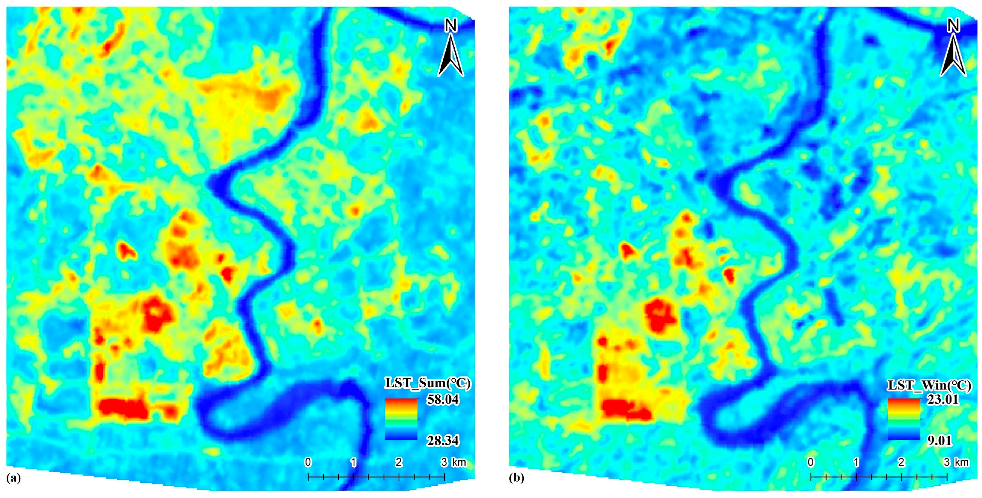
Figure 4a,b depict the LST during summer and winter, respectively. The LST ranged from 28.34 °C to 58.04 °C during summer and from 9.01 °C to 23.01 °C during winter. Upon analyzing Figure 3a,b and Figure 4a,b, we observed that in summer, high LST values are primarily concentrated in the central and western regions, predominantly encompassing industrial, commercial, institutional, residential, and open space. In winter, the high LST areas are predominantly located in the central and southwestern regions, mainly comprising industrial, unused land, agricultural, and green space. To gain a deeper understanding of the spatial distribution variations between different land covers, UFZs, and LST, we conducted a thorough analysis by calculating the difference in average LST between various land covers and UFZs, both in summer and winter, compared to the overall average LST of the study area, at both the grid level and block level.
Figure 5 illustrates the distribution of the differences in average LST between various land covers or UFZs and the entire study area during summer and winter. As depicted in Figure 5a,b, during summer, the average LST of building land, roads, and bare soil is notably higher than the average LST of the entire study area, particularly for building land and roads. Conversely, the average LST of cropland, grassland, woodland, and water is significantly lower than the average LST of the entire study area, with water and woodland exhibiting the most substantial differences. In winter, the average LST of building land, bare soil, roads, cropland, and grassland remains higher than the average LST of the entire study area; however, the average LST of water and woodland, though still lower than the entire study area, experiences a less significant decrease compared to summer. This pattern suggests the presence of spatial distribution variations in LST among different land covers. Furthermore, ANOVA testing revealed a significant difference in LST among various land covers, with a p-value of less than 0.05. Figure 5c,d present the distribution of differences in average LST between UFZs and the entire study area in summer and winter. In summer, the average LST of residential, commercial, industrial, institutional, open space, and unused land zones is observed to be above the entire study area, with industrial exhibiting the most significant difference. Conversely, in winter, within built-up zones, the average LST is lower than the entire study area, excluding industrial. In non-built-up zones, the average LST of unused land and green space is higher, while that of water and agricultural is lower than the entire study area, particularly for water. This indicates spatial distribution differences in LST among different UFZs. Additionally, ANOVA testing confirms these significant differences, with a p-value of less than 0.05.

3.2. Correlation Between 2D/3D UMPs and LST

3.2.1. Pearson Correlation Analysis Results Between 2D UMPs and LST at Grid Level and Block Level

Table 5 presents a comprehensive overview of the Pearson correlation analysis conducted between 2D UMPs and LST at the grid level during summer and winter. The statistical results reveal that the majority of 2D UMPs exhibit a noteworthy correlation with LST. During summer, 2D UMPs related to building land and roads display a pronounced positive correlation with LST. Notably, PLAND_BL (r = 0.365, p < 0.01), COHESION_BL (r = 0.305, p < 0.01), and FRAC_AM_BL (r = 0.281, p < 0.01) indicate significant positive correlations. Specifically, a higher proportion of building area, more complex building shapes, and tighter integration of buildings contribute substantially to an increase in LST. FRAC_AM_RD (r = 0.219, p < 0.01) and COHESION_RD (r = 0.223, p < 0.01) suggest that more complex road shapes and closer integration of roads are significantly associated with increased LST. Conversely, the 2D UMPs of cropland, grassland, woodland, and water show significant negative correlations with LST. Notably, PLAND_WL (r = −0.186, p < 0.01), COHESION_WL (r = −0.13, p < 0.01), PLAND_WT (r = −0.252, p < 0.01), and PLAND_WT (r = −0.224, p < 0.01) indicate that larger coverage areas of woodland or water and the closer integration of these patches are more likely to mitigate the rise in summer LST. Although cropland and grassland contribute to reducing LST, their Pearson correlation coefficients are relatively small, indicating a less pronounced effect compared to woodland and water. Additionally, most of the 2D UMPs of bare soil exhibit a significant positive correlation with LST to varying degrees. Although the r values are relatively small, bare soil still has a noticeable effect on increasing LST.
In winter, the 2D UMPs of building land and roads continue to demonstrate a notable warming effect on LST, albeit weaker compared to summer. Among these factors, COHESION_BL (r = 0.107, p < 0.01), FRAC_AM_RD (r = 0.13, p < 0.01), and COHESION_RD (r = 0.13, p < 0.01) exhibit relatively strong correlations, suggesting that a more cohesive or clustered arrangement of buildings or roads is more conducive to increasing LST in winter. The 2D UMPs of bare soil, cropland, and grassland exhibit a notable positive correlation with LST in winter. Specifically, the UMPs of cropland and grassland have a diametrically opposed influence on LST during winter compared to summer. This reversal is attributed to the substantial reduction in vegetation coverage in winter, which reveals bare ground in many cropland and grassland areas. Consequently, these areas absorb more heat during the day in winter. The impact of bare soil and grassland on LST is more significant than that of cropland, as evidenced by the high correlation coefficients such as COHESION_BS (r = 0.252, p < 0.01) and FRAC_AM_BS (r = 0.244, p < 0.01) for bare soil, and COHESION_GL (r = 0.291, p < 0.01) and FRAC_AM_GL (r = 0.288, p < 0.01) for grassland. This suggests that the intricate distribution and tighter clustering of bare soil or grassland patches play a more favorable role in regulating LST. In winter, woodland and water exhibit a significant negative correlation with LST. However, the absolute value of the correlation coefficient (r) for woodland is comparatively smaller, indicating a reduced cooling effect. This attenuation is attributed to the loss of foliage during winter, which allows for increased direct sunlight penetration and weakened transpiration, thereby reducing heat consumption. Conversely, the larger coverage area and tighter clustering of water, as indicated by PLAND_WT (r = −0.218, p < 0.01) and COHESION_WT (r = 0.191, p < 0.01), result in a more significant reduction in LST.
Table 6 shows the Pearson correlation analysis results between 2D UMPs and LST at the block level during summer and winter. Notably, a majority of the 2D UMPs exhibit a significant correlation with LST. Specifically, in summer, the 2D UMPs pertaining to building land and roads maintain a positive correlation with LST, highlighting UMPs such as PLAND_BL (r = 0.567, p < 0.01) and ED_BL (r = 0.315, p < 0.01) for building land and PLAND_RD (r = 0.221, p < 0.01) and ED_RD (r = 0.194, p < 0.01) for roads. These UMPs indicate that an increased coverage area and density of buildings or roads within a block are likely to contribute to a rise in LST. The 2D UMPs of cropland, grassland, woodland, and water all exhibit a distinct negative correlation with LST. Specifically, LSI_CL (r = −0.256, p < 0.01) and PLAND_CL (r = −0.243, p < 0.01) for cropland reveal that the expansion of cropland coverage area and its more dispersed distribution contribute to a reduction in LST. Additionally, LSI_GL (r = −0.244, p < 0.01) and SHA_AM_GL (r = −0.159, p < 0.01) for grassland suggest that a fragmented grassland distribution also favors a decrease in LST. Similarly, for woodland, PLAND_WL (r = −0.301, p < 0.01), LSI_WL (r = −0.235, p < 0.01), and SHA_AM_WL (r = −0.235, p < 0.01) display a marked correlation with LST, indicating that a larger woodland coverage area and a more irregular shape effectively mitigate LST. Furthermore, LSI_WT (r = −0.413, p < 0.01) and SHA_AM_WT (r = −0.389, p < 0.01) for waterbodies highlight that a more irregular and complex distribution of water significantly enhances their ability to reduce LST. On the other hand, the FRAC_AM and ENN_MN of bare soil do not exhibit a significant correlation with LST at the 0.05 or 0.01 significance levels. However, their LSI, ED, and PD exhibit a strong negative correlation with LST, suggesting that a more fragmented distribution of bare soil is likely to contribute to a decrease in LST.
The influence of 2D UMPs on LST in building land undergoes a notable shift during winter. PLAND maintains a positive correlation, while PD, ED, LSI, and SHA_AM exhibit a negative correlation. Specifically, LSI_BL (r = −0.194, p < 0.01) and ED_BL (r = −0.188, p < 0.01) reveal that more fragmented and irregular building layouts can reduce LST. Conversely, the UMPs of roads have a significantly diminished impact on LST, with PD_RD (r = −0.146, p < 0.01) suggesting that a higher density of road patches in a neighborhood promotes faster heat dissipation, thereby effectively lowering LST. The UMPs of bare soil demonstrate a robust correlation with LST, where PLAND_BS (r = 0.361, p < 0.01) and SHA_AM_BS (r = 0.339, p < 0.01) suggest that a larger coverage area and more complex shape of bare soil in winter enhance its capacity to absorb heat, subsequently raising LST. In cropland, only ED, LSI, SHA_AM, FRAC_AM, and COHESION exhibit significant positive correlations, with ED_CL (r = 0.206, p < 0.01) and SHA_AM_CL (r = 0.166, p < 0.01) indicating that a larger number of cropland patches and more intricate shapes are conducive to increasing LST. In grassland, except for PLAND and PD, which exhibit significant positive correlations, other UMPs do not show a noteworthy relationship with LST. Notably, the 2D UMPs of woodland and water maintain a strong cooling effect in winter, with PLAND and ED remaining the most significant UMPs. This underscores that in winter, a greater coverage area of vegetation or water, along with a higher number of patches, is more effective in reducing LST.

3.2.2. Pearson Correlation Analysis Results Between 3D UMPs and LST at Grid Level and Block Level

Table 7 presents the results of a Pearson correlation analysis between 3D UMPs and LST at the grid level in both summer and winter. Our findings reveal that a significant correlation exists between most 3D BUMPs and 3D TUMPs with LST, regardless of the season. Specifically, in summer, with the exception of BSC, which shows no significant correlation with LST, all other UMPs exhibit significant correlations. Among these, BSVF (r = −0.326, p < 0.01) indicates that an increase in the open space around buildings during summer favors a decrease in LST. Additionally, PBSA (r = 0.31, p < 0.01), PBV (r = 0.335, p < 0.01), and BED (r = 0.31, p < 0.01) suggest that a larger surface area and volume proportion of buildings in 3D space are conducive to an increase in LST. Further, BSA (r = 0.231, p < 0.01) and BVR (r = 0.225, p < 0.01) also exhibit a strong positive correlation with LST, indicating that the surface area and volume of buildings positively impact LST. Regarding the height variation in buildings, BMH (r = 0.215, p < 0.01), BMaH (r = 0.201, p < 0.01), and BHR (r = 0.187, p < 0.01) demonstrate that taller buildings with a greater difference in height are more effective at absorbing solar energy, thereby leading to an increase in LST. Meanwhile, BHV (r = 0.154, p < 0.01) and NBHV (r = 0.207, p < 0.01) indicate that a more dispersed height distribution of buildings tends to enhance LST. However, the r values of BHW and BHL, although slightly smaller than other BUMPs, still suggest a positive correlation with LST improvement. However, in winter, the influence of 3D BUMPs on LST is significantly diminished. Specifically, PBV (r = 0.13, p < 0.01) and BED (r = 0.109, p < 0.01) exhibit a relatively strong correlation with LST, suggesting that an increased volume proportion and Edge Density of buildings in 3D space contribute positively to the rise in LST. Conversely, the height variation in buildings, including BMaH, BHV, NBHV, and BHR, demonstrates a negative correlation with LST. This indicates that taller buildings with greater height differences and a more unstable height distribution are more effective at reducing heat accumulation and accelerating the convection of cold air in winter, ultimately leading to a decrease in LST. Furthermore, BHW, BHL, BLSI, and BSVF also exhibit a negative correlation with LST, further indicating that taller buildings with more complex shapes in 3D space and wider surrounding views are more conducive to the timely dissipation of LST in winter, thereby reducing heat accumulation and lowering LST. In contrast, BSA and BSC do not show a significant correlation with winter LST at the grid level.
Based on the Pearson correlation analysis results of 3D TUMPs and LST in summer, it is evident that all TUMPs except TSC exhibit a significant negative correlation with LST. Specifically, PTSA (r = −0.189, p < 0.01), PTV (r = −0.19, p < 0.01), TED (r = −0.183, p < 0.01), and TLSI (r = −0.155, p < 0.01) suggest that the larger the proportion of Tree Surface Area and Volume in 3D space, and the more irregular and fragmented the shape, the more effective they are in reducing LST. This is attributed to the fact that the greater the proportion of Tree Surface Area and Volume in 3D space, the higher the vegetation coverage, making them more resistant to direct sunlight during summer days. Additionally, the more irregular and fragmented shapes further contribute to reducing LST. Similarly, TSA (r = −0.182, p < 0.01) and TV (r = −0.161, p < 0.01) also exhibit a strong negative correlation. Moreover, the height variation in trees, including TMH (r = −0.1, p < 0.01), TMAH (r = −0.103, p < 0.01), THV (r = −0.1, p < 0.01), NTHV (r = −0.1, p < 0.01), and THR (r = −0.104, p < 0.01), indicates that taller trees, greater height variation between trees, and a more unstable height distribution are all beneficial for reducing LST. This is because while tree coverage effectively resists direct sunlight, height variation enhances air circulation, further accelerating the dissipation of LST. In winter, despite the fact that all TUMPs, apart from TSC, maintain a significant correlation with LST at the 0.01 level, the magnitude of their influence on LST is notably diminished compared to summer. This suggests that while the parameters retain a certain degree of relevance, their efficacy in modulating LST during the colder season is substantially reduced.
Table 8 presents the comprehensive findings of the Pearson correlation analysis conducted to examine the relationship between 3D UMPs and LST at the block level, spanning both summer and winter. The results highlight a significant correlation between the majority of 3D UMPs and LST. More precisely, in summer, PBSA (r = 0.384, p < 0.01), BED (r = 0.374, p < 0.01), and BLSI (r = 0.374, p < 0.01) emerge as pivotal factors exerting a considerable impact on LST. This underscores the significance of the buildings’ surface area ratio in the 3D space, their fragmented distribution, and the complexity of their shapes in contributing significantly to the rise in LST at the block level during summer. The influence of PBV (r = 0.068, p < 0.01) has notably diminished. Conversely, BSA (r = 0.178, p < 0.01) and BVR (r = 0.253, p < 0.01) continue to exhibit a robust positive correlation with LST. As we delve into the effect of variations in building height, BMH (r = 0.208, p < 0.01), BMaH (r = 0.117, p < 0.01), and BHR (r = 0.117, p < 0.01) suggest that a rise in building height and its heterogeneity tend to exacerbate the increase in LST. While BHV (r = 0.083, p < 0.01) and NBHV (r = 0.021, p < 0.01) still have a positive correlation, their impact on LST is substantially less significant. Furthermore, BHL (r = 0.295, p < 0.01) and FAI (r = 0.254, p < 0.01) indicate that a larger frontal area of buildings enhances solar energy absorption, thereby contributing significantly to the rise in LST. In contrast, BSVF (r = −0.365, p < 0.01) shows a marked negative correlation with LST, implying that a more open visual perspective of buildings in a block, coupled with less building aggregation, facilitates faster air convection and significantly mitigates the increase in LST. Notably, BHW and BSC do not demonstrate a significant correlation with LST. During winter, the variation in building height exhibits a stronger correlation with LST compared to other BUMPs. Specifically, BMH (r = −0.223, p < 0.01), BMaH (r = −0.278, p < 0.01), BHR (r = −0.278, p < 0.01), BHV (r = −0.315, p < 0.01), and NBHV (r = −0.235, p < 0.01) all indicate that taller buildings, greater height differences, and uneven height distribution enhance the convection of cold air during the day in winter. Even if some solar heat is absorbed, it is quickly dissipated. Additionally, the taller the buildings, the more shadows they cast, blocking solar energy and leading to a decrease in LST. On the other hand, BSVF (r = 0.289, p < 0.01) exhibits a positive correlation with LST in winter. Meanwhile, PBSA (r = −0.186, p < 0.01), PBV (r = −0.223, p < 0.01), BSA (r = −0.167, p < 0.01), and FAI (r = −0.163, p < 0.01) suggest that larger surface and frontal areas, as well as a greater proportion of surface area and volume in 3D space, block more solar energy from reaching the interiors of buildings. This, coupled with the smaller solar elevation angle in the northern hemisphere during the daytime in winter, contributes to a reduction in LST within the block. BV, BHL, BED, and BLSI also demonstrate a negative correlation with LST, albeit to a lesser extent. Lastly, BSC does not exhibit a significant correlation with LST.
For 3D TMUPs, during summer, PTV (r = −0.315, p < 0.01), PTSA (r = −0.286, p < 0.01), TSA (r = −0.271, p < 0.01), and TV (r = −0.262, p < 0.01) show a strong negative correlation with LST. This signifies that the greater the surface area and volume of trees in the block level, along with their larger proportion in 3D space, the more effective they are at blocking direct solar heat. Furthermore, the transpiration process of vegetation accelerates the dissipation of heat. TLSI (r = −0.212, p < 0.01) suggests that a more irregular distribution of trees in 3D space is favorable for reducing LST. Furthermore, the parameters TMH, TMaH, and THR, as well as the height variations THV and NTHV, also exhibit a strong negative correlation with LST. This indicates that taller trees and a more uneven distribution of tree heights at the block level result in a larger surface area blocking direct sunlight. Additionally, the uneven distribution of tree heights enhances air circulation, further accelerating the dissipation of heat. Based on the Pearson correlation analysis between 3D TUMPs and LST during winter, certain parameters exhibit a greater influence on LST compared to summer, contrasting with the grid-level findings. Specifically, TMH (r = −0.437, p < 0.01), THV (r = −0.427, p < 0.01), and TLSI (r = −0.429, p < 0.01) have the most significant impact on LST. This is attributed to the change in solar elevation angle during winter, which significantly reduces the energy reaching the ground in the northern hemisphere. Trees with a higher average height, more unstable height variation, and a more irregular distribution are more likely to block the weakened winter solar energy, resulting in a shadow effect that reduces LST [55]. Additionally, TMaH (r = −0.354, p < 0.01), THR (r = −0.35, p < 0.01), PTSA (r = −0.354, p < 0.01), and PTV (r = −0.308, p < 0.01) also demonstrate a strong negative correlation with LST, indicating that taller trees, greater height differences, and a larger proportion of surface area and volume in 3D space are more likely to a lower LST in winter. In contrast, NTHV, TSA, and TV have a relatively weaker impact on LST, yet they still exhibit a significant negative correlation.
3.3. Regression Analysis Between 2D and 3D UMPs and LST

Table 9 summarizes the R2 statistical results of multiple linear regression models that investigate the correlation between UMPs and LST in both the entire study area and built-up zones during summer and winter. Among the seven regression models for summer, when assessing the impact of individual 2D or 3D UMPs as input variables (Mod.1 to Mod.3), 2D UMPs emerge as the most influential factor on LST, outperforming 3D UMPs in explaining LST variations, except in the commercial zones. In the entire study area, the explanatory power of 2D UMPs reaches 65.2%. In various zones, 2D UMPs also show strong explanatory power, achieving a 62.6% explanatory power in industrial zones. Additionally, in the residential, commercial, industrial, and institutional zones, 3D BUMPs demonstrate a greater explanatory power compared to 3D TUMPs. However, in open spaces, 3D TUMPs excel in explaining LST changes, surpassing 3D BUMPs. Notably, within the commercial zone, 3D BUMPs possess outstanding explanatory power for LST changes, accounting for 50.8% of the variations. In industrial zones, 3D TUMPs exhibit the strongest explanatory power for regression models, with a noteworthy R2 of 32.4%. The statistical results from the regression modeling of LST, utilizing a combination of 2D and 3D UMPs (Mod.4 to Mod.7), reveal the diverse explanatory strengths of various model configurations across the entire study area and built-up zones. Mod.4, integrating 2D UMPs with 3D BUMPs, displays robust explanatory power, achieving R2 values spanning from 49.7% to 68.6%. Its performance is particularly pronounced in the entire study area and industrial zones, where R2 values exceed 60%. While Mod.5, combining 2D UMPs with 3D TUMPs, has a lower impact on LST changes compared to Mod.4, it still exhibits satisfactory explanatory power ranging from 46% to 67.4%. Mod.6, which incorporates 3D BUMPs and TUMPs, shows relatively weaker performance overall, especially in open spaces where the R2 value stands at just 17.9%. However, in commercial zones, it outperforms Mod.5 in explaining LST variations. The standout model is Mod.7, which incorporates all 2D and 3D UMPs as independent variables. It demonstrates the utmost explanatory power, with R2 values surpassing 50% across the entire study area and built-up zones. Notably, the R2 values for the entire study area and industrial zones reach 70.9% and 71.3%, respectively, indicating an excellent model fit. This outcome underscores that the interplay between 2D and 3D UMPs more accurately captures the fluctuations in LST.
In the winter, the R2 statistical results of Mod.1 to Mod.3 indicate that 2D UMPs exert a more significant influence on LST compared to 3D BUMPs and TUMPs in the entire study area, industrial zones, institutional zones, and open spaces. Specifically, within industrial zones and the entire study area, the explanatory power of 2D UMPs in explaining LST changes reaches 62.9% and 50%, respectively. Conversely, while 3D BUMPs demonstrate a greater influence on LST variations in residential and commercial zones than 2D UMPs and 3D TUMPs, their explanatory strength for LST changes remains relatively modest, attaining only 30.4% and 27.2%, respectively. Interestingly, 3D TUMPs exhibit a more pronounced impact on LST in open spaces compared to 3D BUMPs. From the R2 statistical outcomes of Mod.4 to Mod.7, Mod.4 achieved better model fitting, with an interpretation ability of 40–66.9% for LST in various regions. Its influence on LST in the entire study area, as well as in residential, commercial, industrial, and institutional zones, surpasses Mod.5 and Mod.6. In open spaces, Mod.5 achieves better model fitting than Mod.4 and Mod.6, highlighting the significant role of 3D TUMPs in these zones. Mod.6 had poor model fitting, with an interpretation ability of only 31.6–57.5% for LST in the entire study area and built-up zones. Although it performed well in industrial zones, it performed poorly in institutional zones. Similar to summer, Mod.7 combined all 2D and 3D UMPs in winter and achieved the highest model fitting, with model interpretation abilities of over 50% for all regions except institutional zones, including 65.7% and 67.6% for the entire study area and industrial zones, respectively. This fully demonstrates the impact of combining 2D and 3D UMPs on LST changes. It is worth noting that in institutional zones, the R2 values of Mod.4 and Mod.7 were both 0.4, indicating that the influence of 3D TUMPs on LST in these zones is diminished when combined with other UMPs. This same phenomenon is also observed in summer.
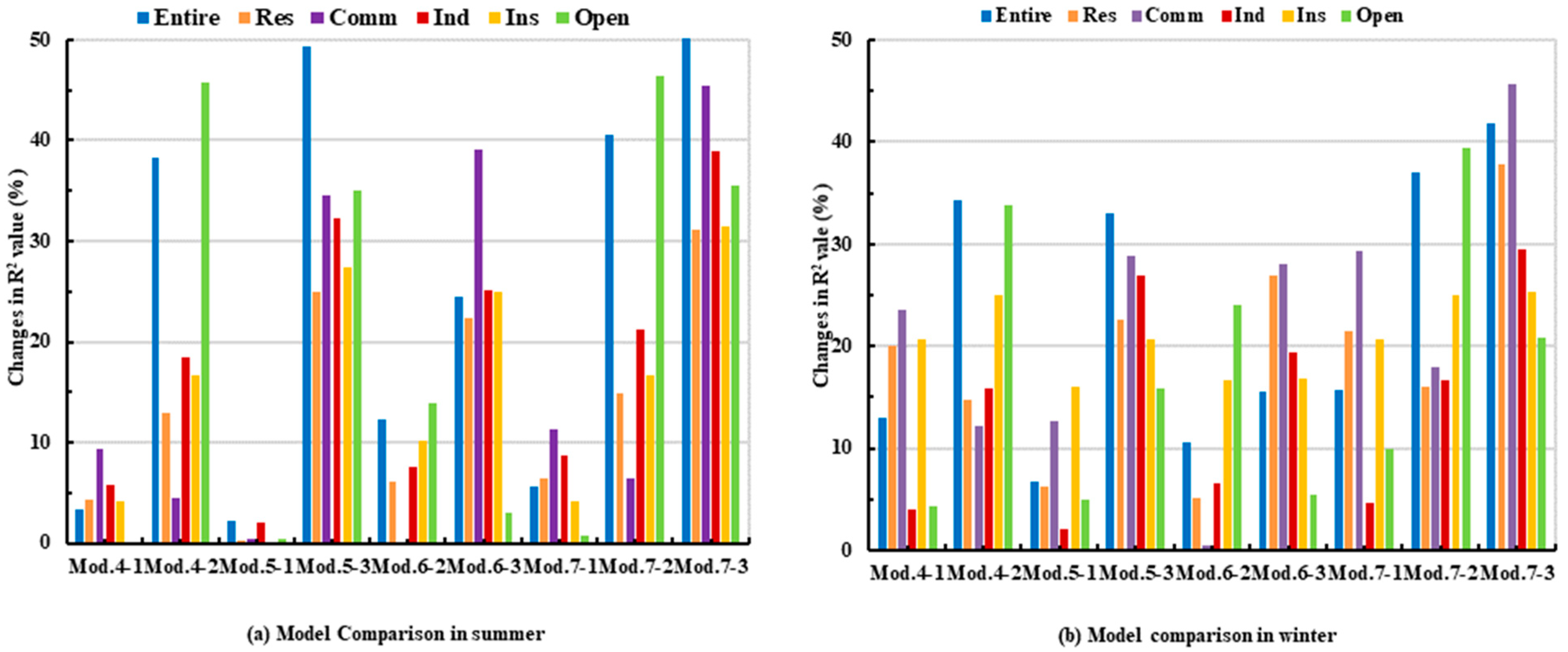
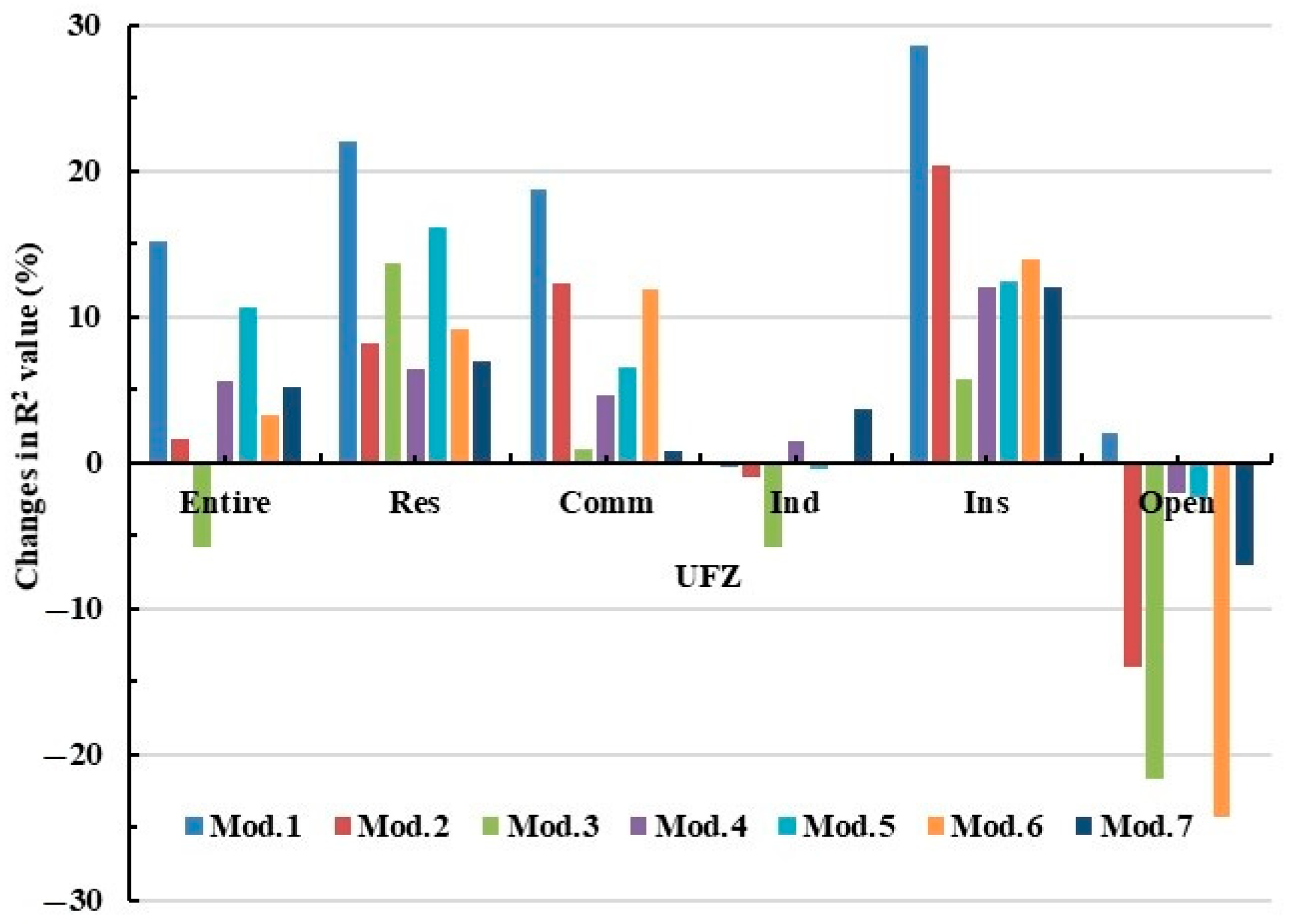
Figure 6 highlights the change in R2 values of regression models when the combined 2D and 3D UMPs are employed as input variables, in contrast to models utilizing a single 2D UMP or 3D UMP. This comparison enables a more thorough evaluation and analysis of how 2D UMPs, 3D UMPs, or their combinations influence the fluctuation of LST. During summer, Mod.4 exhibits a substantially greater influence on LST compared to Mod.1 and Mod.2, notably outperforming Mod.2, which solely utilizes 3D BUMPs as input variables. The improvement is particularly significant, with the R2 values for the entire study area and open spaces increasing by 38.3% and 45.7%, respectively. Additionally, the improvement over Mod.1 ranges from 0.1% to 9.3%, further validating the superiority of 2D UMPs in explaining LST variations compared to 3D BUMPs. Analyzing the changes in R2 values between Mod.5, Mod.1, and Mod.3, the improvements observed in the entire study area and built-up zones indicate that the integration of 2D UMPs and 3D TUMPs significantly outperforms Mod.3, which relies solely on 3D TUMPs. The improvement ranges from 25% to 49.3%. In contrast, the enhancement, compared to Mod.1, is more modest, and the R2 value in institutional zones remains stable. This underscores two key points: Firstly, 2D UMPs exert a more substantial influence on LST than 3D TUMPs. Secondly, 3D TUMPs appear to have a negligible effect on LST in institutional zones during summer, which explains the similarity in R2 values between Mod.4 and Mod.7 in institutional zones.
Upon analyzing the changes in R2 values between Mod.6, Mod.2, and Mod.3, it becomes evident that the integration of 3D BUMPs and TUMPs exerts a more significant influence on LST compared to Mod.3, which relies solely on 3D TUMPs. In the entire study area, as well as in residential, commercial, industrial, and institutional zones, the R2 values showed a rise of 22.3–39.1%, clearly indicating that 3D BUMPs possess a stronger explanatory power for LST compared to 3D TUMPs. However, considering that open spaces are predominantly vegetated with trees, the influence of 3D TUMPs on LST in these areas is notably more significant than 3D BUMPs. When compared to regression models that utilize either 2D or 3D UMPs as input variables, Mod.7 demonstrates a more significant enhancement in explanatory power for LST. Specifically, it elevates R2 values by 0.8–11.3% compared to Mod.1, 6.5–46.4% compared to Mod.2, and 31.1–52.8% compared to Mod.3. This underscores the notion that the combined utilization of 2D UMPs, 3D BUMPs, and 3D TUMPs significantly improves the ability to explain variations in LST.
In winter, Mod.4 significantly enhances the fitting capability of the model compared to Mod.1 and Mod.2, particularly when contrasted with Mod.2, which solely relies on 3D BUMPs. The R2 value experiences a notable rise of 12.2–34.3%, clearly indicating that 2D UMPs possess a stronger explanatory power for LST than 3D BUMPs. Similarly, Mod.5 demonstrates a substantial improvement in its effect on LST compared to Mod.1 and Mod.3, with a particularly pronounced enhancement when benchmarked against Mod.3, achieving an R2 value increase of 15.8–33%. This underscores the greater influence of 2D UMPs on LST compared to 3D TUMPs. When considering the differences in R2 values between Mod.6 and Mod.3 (referred to as Mod.6–3) and Mod.6 and Mod.2 (referred to as Mod.6–2), it becomes evident that the entire study area and residential, commercial, industrial, and institutional zones experience a more significant R2 value increase in Mod.6–3 than in Mod.6–2. This indicates that buildings exert a greater influence on LST than trees in these areas. Furthermore, the larger change in open spaces observed in Mod.6–2 compared to Mod.6–3 underscores the crucial role of trees in open spaces in affecting LST. Mod.7, which incorporates all 2D and 3D UMPs, significantly elevates the fitting degree of regression models compared to those utilizing single input variables. This further strengthens the argument that the combined utilization of 2D and 3D UMPs plays a pivotal role in affecting LST. Specifically, Mod.7 exhibits an LST impact that is 4.7–29.3% higher than Mod.1, 16.1–39.4% higher than Mod.2, and 20.8–45.6% higher than Mod.3. This data comparison underscores the superiority of 2D UMPs in explaining LST variations, followed by 3D BUMPs and then 3D TUMPs.

3.4. Relative Importance of UMPs for LST

Table 10 illustrates the distribution of β values, reflecting the relative importance of each UMP in relation to LST in the multiple linear stepwise regression model for both summer and winter. Evidently, from the table, when considering the comprehensive influence of all 2D and 3D UMPs on LST, 35 UMPs demonstrate a noteworthy impact on LST during summer (p < 0.05). In terms of the β value distribution of 2D UMPs, building land, bare soil, and roads emerge as primary warming factors in summer. Composed of materials with low heat capacity, such as steel, cement, concrete, and gravel, these land covers absorb more heat in summer, elevating LST. Notably, the area proportion of building land (PAND_BL, β = 0.898) has the most significant effect on LST. Parameters like COHESION_BL (β = 0.198), FRAC_AM_BL (β = −0.183), ED_BL (β = −0.179), and SHA_AM_BL (β = 0.074) further emphasize that a more concentrated and regular distribution of buildings contributes to an increase in LST. The influence of bare soil on LST, represented by the PLAND (β = 0.353), ED (β = −0.204), and SHA_AM (β = 0.095), indicates that a larger and more regularly shaped area of bare soil leads to increased heat absorption and, consequently, a higher LST. Similarly, road UMPs, specifically PLAND (β = 0.3) and PROX_MN (β = 0.05), suggest that a larger road surface area and closer proximity between adjacent roads contribute to greater heat accumulation, further elevating LST. Additionally, the landscape factor SHDI (β = 0.116) associated with each block reveals a positive correlation between landscape diversity and LST. In contrast, cropland, grassland, and woodland emerge as essential cooling factors during summer. Their dense green vegetation coverage not only shields most direct sunlight but also promotes heat dissipation through enhanced daytime transpiration. The SHA_AM (β = 0.105) of cropland suggests that a more complex shape can contribute to a reduction in LST. The PLAND (β = −0.189), LSI (β = −0.091), and FRAC_AM (β = −0.044) of grassland indicate that a larger area, more regular shape, and fragmented distribution are associated with a decrease in LST. Notably, the LSI (β = −0.129) of woodland also exhibits a significant cooling effect. Water serves as a crucial cooling factor due to its high heat capacity. It absorbs less heat compared to other land covers, and during summer, water evaporation intensifies, consuming surrounding heat and thus reducing LST. The LSI (β = −0.166), ED (β = −0.088), and PD (β = −0.085) of water underscore their importance in LST reduction, highlighting that a more regular shape and concentrated distribution are more effective in mitigating LST. The impact of 3D BUMPs and TUMPs on LST is significant. Notably, the BSVF of buildings (β = −0.306) is particularly important. In summer, a more open view of buildings enhances air convection, thereby lowering LST. PBSA (β = −0.202) and BED (β = −0.264) also significantly affect LST, indicating that in a 3D space, more densely packed and less fragmented buildings absorb more heat, leading to an increase in LST. Additionally, smaller variations in building height (BHV, β = −0.14) and larger building volumes (BV, β = −0.094) contribute to raising LST. The relative importance of 3D TUMPs on LST is primarily manifested in variations in height, volume, and shape. The TMH (β = −0.141), NTHV (β = −0.045), and THR (β = −0.044) indicate that the taller and more stable in height the trees are, the better they can block solar heat. TV (β = −0.087) suggests that larger Tree Volumes and denser foliage enhance transpiration, thereby consuming more heat and lowering LST. Conversely, the TED (β = 0.12) shows that the more fragmented the spatial distribution of trees, the less effective they are at cooling LST.
In the winter regression model, 28 UMPs significantly impact LST (p < 0.05). The distribution of β values for 2D UMPs underscores the continued significance of building land and bare soil as primary factors contributing to the rise in LST during winter. However, unlike in summer, road UMPs do not exhibit a significant influence on LST in winter. Conversely, related 2D UMPs for grassland demonstrate a positive correlation with LST. The PLAND of building land, with a β value of 0.767, stands out as the most influential factor on LST. Additionally, the PLAND (β = 0.267) and ED (β = −0.187) of bare soil also play crucial roles, indicating that larger areas of buildings and bare soil and more regular shapes of bare soil contribute to a higher LST. Similarly, the larger areas of grassland (PLAND, β = 0.079) and more irregular shapes (SHA_AM, β = −0.107) lead to a higher LST. This can be attributed to the significantly reduced grassland vegetation cover during winter, leaving exposed surfaces to absorb more heat. Furthermore, the LSI of cropland, with a β value of 0.155, also significantly impacts LST. For woodland, the PD and LSI values indicate that a more fragmented distribution and irregular shapes significantly diminish its cooling effect on LST. In contrast, most UMPs of water maintain a robust negative correlation with LST during winter. However, an exception is observed in the FRAC_AM (β = 0.196), which suggests that water with more irregular shapes tends to have a higher LST. Furthermore, the SHDI (β = 0.079) continues to exhibit a positive correlation with LST in winter.
Based on the statistical of the relative importance β values between 3D UMPs and LST, it is evident that the BSVF (β = 0.491) exhibits a robust positive correlation with winter LST. This correlation is attributed to the fact that during winter, buildings with a wider view capture a larger area of solar energy. Conversely, a reduced BSVF signifies increased obstruction among buildings, leading to the formation of shadows that diminish the capacity of the ground to receive solar energy, thereby causing a decline in LST. Likewise, the BHL (β = −0.149) underscores the significance of reduced obstruction surrounding buildings. The BMH (β = 0.256) and BHV (β = −0.322) provide insights into how building height affects LST. Specifically, taller buildings with minimal variation in their heights contribute favorably to an increase in LST. The BED (β = −0.33) suggests that a higher degree of fragmentation in the 3D arrangement of buildings hinders heat accumulation during winter, leading to a decrease in LST. However, the PBV (β = 0.084) exhibits a relatively minor influence on LST. Among the 3D TUMPs, the TLSI (β = −0.254) emerges as the most significant factor influencing LST variations. This indicates that trees with more irregular leaf shapes are more effective in reducing LST. Additionally, the TMH (β = −0.18) and TED (β = 0.159) provide further insights. Specifically, taller trees tend to reduce LST, while a lower degree of fragmentation in the 3D space occupied by trees also increases the likelihood of a decreased LST. For 3D TUMPs, the most important factor affecting LST changes is the TLSI (β = −0.254), indicating that the more irregular the shape of the trees, the more effective it is to reduce LST. The TMH (β = −0.18) and TED (β = 0.159) indicate that the higher the height of trees, the smaller the degree of fragmentation in 3D space, making it more likely to reduce LST.
We conducted a further analysis of the percentage of the absolute β value within the total absolute β value for UMPs in both summer and winter, aiming to assess the relative importance of 2D and 3D UMPs on LST. Figure 7 depicts the distribution of these percentages for 2D and 3D UMPs across the two seasons. The figure reveals that regardless of the season, 2D UMPs exhibit greater importance on LST compared to 3D UMPs. Specifically, in summer, among the 35 UMPs, 2D UMPs account for 72.36% of the total relative importance, while 3D UMPs, though comprising 27.64%, still play a crucial role in influencing LST. In winter, with 28 UMPs considered, the relative importance of 3D UMPs rises significantly, accounting for 43.5% of the total, thus emphasizing the significance of 3D UMPs. Moreover, in comparing the importance of 3D BUMPs and TUMPs, we observed that 3D BUMPs outweighed 3D TUMPs in both summer and winter. Nevertheless, 3D TUMPs also possess significant relative importance, accounting for 8.37% and 12.16% in summer and winter, respectively, making them an indispensable factor in our research.

4. Discussion

4.1. Influence of 2D and 3D UMPs on LST at Grid Level and Block Level

Understanding the driving forces behind changes in LST is crucial for improving the urban thermal environment. Prior research has demonstrated that urban morphology significantly influences LST, yet most studies have concentrated on large cities, leaving SMSCs relatively under-explored. Furthermore, there is insufficient exploration of the impact of 3D urban morphologies on LST in SMSCs [24,56]. Therefore, we selected Ziyang as our study area, utilized high-resolution remote sensing data to extract refined UMPs, and investigated the impact of both 2D and 3D UMPs on LST during summer and winter at both the grid level and block level. Then, we conducted a comprehensive analysis and discussion on the relationship between seven land covers and nine UFZs regarding their impact on LST changes. Previous studies have inadequately addressed the individual effects of roads, grasslands, and trees on LST, and the types of UFZs have not been thoroughly considered [14,56,57,58]. In addition, we comprehensively evaluated the 2D landscape pattern composition, spatial configuration, and degree of fragmentation of land covers, as well as the spatial distribution, variation, and interrelationships of 3D buildings and trees. We extracted 38 distinct 2D and 3D UMPs to provide a more detailed analysis and interpretation of the changes in LST. Our findings reveal that 2D and 3D UMPs exhibit a significant correlation with LST in SMSCs, regardless of the season. These correlations demonstrate the similarities and differences at the grid level and block level.
By comparing and analyzing Table 5 and Table 6, we discovered that at the grid level, the 2D UMPs of building land (PLAND, COHESION) and roads (FRAC_AM, COHESION) significantly increase summer LST but show minimal winter impact, consistent with previous findings [14]. While grassland and cropland provide summer cooling, they exhibit winter warming effects, particularly grassland, which substantially enhances LST. Woodland and water consistently demonstrate cooling effects (summer > winter), confirming vegetation and water as primary summer cooling factors [34,59,60]. Bare soil shows weak summer correlations but strong winter warming, with all correlation coefficients notably increasing, indicating a substantial impact on LST [14]. Furthermore, our grid-level analysis of the 2D UMPs showed a relatively strong relationship between the PLAND, FRAC_AM, and COHESION indices and LST. This finding indicates that at the 30 m grid level, the primary factors affecting LST are the coverage, shape complexity, and density and connectivity of land covers. For urban planning, these results suggest prioritizing (1) strategic placement of woodland and water in areas with high building density, (2) optimizing grassland distribution to balance seasonal thermal effects, and (3) regulating bare soil exposure through temporary vegetation cover during winter months. Such measures would effectively mitigate the UHI effect while addressing seasonal thermal variations.
In the block-level analysis, the 2D UMPs of building land demonstrate a notably strong positive correlation with LST in summer, outperforming the correlation observed at the grid level. Conversely, in winter, this correlation is substantially weakened. However, in winter, it is worth noting that the 2D UMPs of building land that measure the degree of landscape fragmentation and complexity exhibit a negative correlation with LST, whereas those indicating the degree of similarity, proximity, and aggregation among patches show no correlation. This finding implies that a dispersed distribution of building land in winter promotes efficient heat dissipation, resulting in lower LST values. The 2D UMPs of bare soil display a consistent positive correlation with LST in both summer and winter, yet their influence is notably stronger in winter than in summer. In contrast, the majority of 2D UMPs for cropland and grassland exhibit a negative correlation with LST during summer. However, in winter, all 2D UMPs for these two land covers show a positive correlation with LST, albeit with a substantial decrease in the quantity of highly correlated UMPs. This seasonal variation highlights the effect of winter vegetation reduction, leading to the exposure of cropland and grassland and enabling them to absorb greater amounts of heat. The thermal influence of road-related 2D UMPs on LST exhibits seasonal patterns similar to building land, with comparable impacts during summer but substantially reduced effects in winter. This seasonal attenuation aligns with the existing literature [14,61] and can be attributed to the low specific heat capacity of road materials, which results in balanced heat absorption and dissipation under winter’s lower temperature conditions, consequently minimizing their thermal influence [62]. In contrast, woodland and water maintain consistent cooling effects across summer and winter at the block level, demonstrating strong negative correlations with LST, as documented in previous studies [59,63]. Our analysis identifies five key 2D UMPs (PLAND, PD, ED, LSI, and SHA_AM) as primary determinants of LST variation, highlighting the significant role of land cover composition (percentage and patch quantity) and spatial configuration (shape and complexity) in impacting LST at the block level. Furthermore, the observation of Table 7 and Table 8 reveals that the influence of 3D UMPs on LST is equally crucial. Our findings reveal that, whether at the grid level or block level, most 3D UMPs of buildings and trees exhibit a significant correlation with LST, which is more prominent compared to their 2D UMPs. Our research analysis results are consistent with Yu et al. (2020) [23] but deviate from previous research conducted by Huang et al. (2019) [14]. We postulate that this discrepancy arises from variations in the 2D and 3D spatial distribution of buildings and trees across different cities. Notably, the most prominent factors influencing LST are the height variation characteristics of buildings or trees, the proportion of surface area and volume they occupy in 3D space, and their degree of irregularity. The BSVF is particularly significant, highlighting the critical role of 3D urban configuration—including building and tree arrangement—in mitigating the UHI effect. BSVF influences LST through two primary mechanisms: (1) higher SVF enhances ventilation by increasing visible sky exposure, thereby improving air circulation and cooling dense urban areas [64]; (2) lower SVF reduces surface heating by limiting solar radiation penetration [65]. The effect of BSVF on LST varies across different due to inconsistent relative intensities of these two processes [15,66,67], which is associated with local climatology, geography, and surface topography of the research locations [68].
The relationship between UMPs and LST is influenced by multiple interacting factors. Our comparative analysis reveals that block-level (vs. grid-level) analysis better captures the spatial distribution of land cover and highlights clearer distinctions among UMPs, enabling deeper insights into their effects on LST. Therefore, we employ block-level regression models to examine how 2D and 3D UMP combinations explain LST variations while also exploring the role of UFZs in SMSCs. As shown in Table 9, combining 2D and 3D UMPs provides a more robust explanation for LST variations across the entire study area and built-up zones, consistent in both summer and winter. This aligns with prior studies [14,42]. However, Yu et al. [23] found that using only 3D UMPs yielded the highest model accuracy in the entire study area and industrial zones, with 2D UMPs offering no improvement—a divergence suggesting context-dependent effects of UMP integration. Our analysis of UMPs’ relative importance to LST identified key 2D and 3D parameters significantly affecting LST in both seasons. Artificial surfaces (e.g., steel, concrete) and natural exposed surfaces (e.g., sandstone, dry soil) substantially increase LST, consistent with previous findings [61,62,63]. For LST mitigation in SMSCs, optimal 3D spatial arrangement of buildings and vegetation is crucial, particularly considering 3D UMPs, including BSVF, BED, PBSA, TMH, and TLSI. Figure 7 demonstrates that 2D UMPs predominantly influence LST in summer, while both 2D and 3D UMPs exhibit comparable effects in winter. Although 3D UMPs represent only 30% of total parameters (28/92), their substantial contribution confirms their critical role in UMP-LST studies, consistent with previous studies emphasizing 3D UMP importance [23,42,69]. These findings underscore two key urban planning recommendations: (1) optimization of 2D landscape layouts and (2) strategic design of 3D building and vegetation configurations (incorporating height, area, shape, and spatial arrangement). This dual approach provides valuable guidance for thermal environment mitigation, livability enhancement, and sustainable urban development in SMSCs.

4.2. Seasonal Stability and Differences in the Impact of UMPs on LST

Based on previous research examining the influence of urban morphology on LST across four seasons, it is evident that summer and winter, as the hottest and coldest seasons, respectively, exhibit the most significant seasonal variations in the effect of urban morphology on LST [14,69]. In this study, we conducted a further comparison of the results obtained from seven regression models presented in Table 9. Additionally, we calculated the R2 values of these models for summer, relative to their corresponding values in winter, which are depicted in Figure 8. Our findings revealed that the influence of various models on LST differs significantly across different functional zones during both summer and winter. We observed that residential, commercial, and institutional zones exhibit a more profound influence on LST in summer compared to winter. Among the regression models for the entire study area, excluding Mod.3, which relies solely on 3D TUMPs as variable inputs, the impact on LST is considerably higher in summer than in winter. This phenomenon is primarily due to the direct sunlight over the Tropic of Cancer during summer, enabling the ground to absorb more heat. Additionally, urban structures, mainly comprising artificial constructs like buildings and roads with high absorption properties, further amplify this effect. Conversely, the lower solar elevation angle in winter significantly reduces the energy reaching the ground. Moreover, the intensified human activities during summer exacerbate this impact, making the summer LST changes more sensitive to the composition, spatial distribution, and human activities associated with the land characteristics in the region. However, the impact is less pronounced in winter, which aligns closely with the findings of several studies [21,70].
Industrial zones are primarily influenced by numerous activities such as processing, manufacturing, and smelting, which generate significant industrial heat. Consequently, they are less susceptible to seasonal variations. Additionally, these zones are often situated in suburban areas distant from urban centers, where the abundant vegetation in summer provides a robust cooling effect. Conversely, in winter, most grasslands and croplands become barren, allowing them to absorb solar energy during the daytime. As a result, we discovered that the influence of certain regression models on LST in industrial zones is slightly more pronounced in winter than in summer. Open spaces, predominantly urban squares or vacant areas, have less tree coverage in winter, leading to a greater area of direct sunlight exposure and increased solar energy absorption. Hence, their impact on LST is higher in winter than in summer. Nonetheless, on a broader scale, the influence of urban morphology on LST is greater in summer than in winter, explaining why most studies tend to focus on the summer season [71,72].

4.3. Implications for Urban Planning and Management

Our research findings indicate that both 2D and 3D urban morphology have a profound effect on the LST in SMSCs during summer and winter. Consequently, to mitigate the adverse effects of thermal environment problems on the urban living environment, it is imperative to prioritize the rational arrangement of buildings, roads, grasslands, and trees in the context of detailed urban planning. Buildings have a profound impact on LST, significantly influencing the absorption of solar radiation, the formation of air currents, and the generation of anthropogenic heat. As the size and concentration of building footprints increase, so does the absorption of solar energy, which in turn impedes air circulation. Consequently, urban planners are encouraged to optimize the spatial layout of urban landscapes by dispersing buildings. However, in urban areas where land resources are scarce, simply reducing the number of buildings is not a feasible solution. Instead, we can rationally modify the aggregation and fragmentation of buildings in 3D spatial structure. Enhancing the variation in building heights and increasing the openness of buildings can foster the generation of air currents. Additionally, reducing the volume of buildings can help alleviate the UHI effect during the daytime. As cities continue to expand, roads proliferate, and the asphalt or cement surfaces they are composed of are highly heat-absorbent. To mitigate this, planners are advised to minimize road density and increase the spacing between adjacent roadways. Grassland and trees play a crucial role in mitigating the UHI effect, thanks to their transpiration and shading capabilities. Their proportion within urban landscapes is a significant factor in influencing and reducing LST. Furthermore, the specific layout and design of grassland and trees also have an impact on LST variations. Given the limited availability of urban green space, dispersing these green elements throughout urban areas serves as an efficient strategy to alleviate the UHI effect. Altering the 3D structure of trees is an effective approach to mitigating the UHI effect. It is advisable to plant a greater number of tall and lush trees while minimizing the height variation between them to block more solar heat and boost transpiration, thereby consuming additional heat. Bare soil also has a significant warming effect; therefore, it is recommended that urban planners increase green vegetation coverage to not only reduce heat radiation absorption but also enhance the urban aesthetic. Water-related urban morphology is a crucial cooling factor. The more regular the shape of the water and the more concentrated its distribution, the more effective it is in reducing LST. Consequently, on one hand, it is essential to strengthen the protection of water, and on the other, it is necessary to standardize the management of rivers, lakes, and other water sources and repair water channels to the greatest extent possible. Additionally, our study reveals the impact of different UFZs on LST, which is conducive to minimizing the effects of urbanization through targeted landscape optimization and land use planning. For instance, in high-density, high-rise commercial and residential zones, greater emphasis should be placed on the design of 3D architectural morphology. Apart from modifying the distribution and design of urban morphology, adjusting the albedo of building and road materials and incorporating green roofs and green facades can also exert a cooling effect on the urban environment [14,73].

4.4. Limitations and Prospects for Future Research

In our investigation of the effects of 2D and 3D UMPs on LST, we focused solely on the diurnal variations in LST, overlooking the potential influence of urban morphology on LST during the nighttime. Additionally, the derived UMPs were not validated through ground-based measurements. Secondly, during the retrieval of LST, the geometric scattering effect of thermal radiation caused by the 3D structural characteristics of cities and the adjacency effect between pixels are not considered. Thirdly, our analysis was limited to grid-level (only 30 m) and block-level scales, overlooking the fact that LST exhibits distinct patterns at varying scales and within different regions. Moreover, the data derived from ALS predominantly captures horizontal surface information, neglecting the significance of facade features like walls on LST, particularly in densely built-up zones. Also, there exists a challenge related to the time gap between the acquisition of airborne LiDAR data and LST data. While the distribution of land cover remains relatively stable in the short term, obtaining precise and timely vegetation information across different seasons poses a significant hurdle. This study exclusively examines linear relationships between UMPs and LST without incorporating machine learning approaches (e.g., random forests, gradient boosting machines, or Extreme Gradient Boosting) [25,72,74] to elucidate potential nonlinear interaction mechanisms. Finally, given the seasonal variations and differences in the spatial distribution of buildings across various cities, our research methodology requires further validation in a broader range of urban settings.
In our future research endeavors, we will systematically investigate the effect of urban morphology on diurnal LST through multi-scale thermal remote sensing (Landsat 8, ASTER, and MODIS) with improved LST retrieval algorithms that account for geometric structure and adjacency effects [75,76]. Seasonal airborne LiDAR acquisitions and field validation will enhance the accuracy of UMPs. An integrated linear and machine learning analytical framework will be employed to balance interpretability with complex pattern recognition, providing mechanistic insights into UMP-LST interactions. Comparative studies across SMSCs with diverse climates, scales, and urban forms will further validate the generalizability of these findings.

5. Conclusions

This study leverages high-resolution remote sensing data to quantify the impacts of 2D and 3D UMPs on LST in SMSCs. The findings highlight critical relationships between urban morphology and the thermal environment, offering actionable strategies for UHI mitigation in urban planning. The research outcomes revealed the following:
Utilizing correlation analysis, we found that 2D UMPs dominate LST variability, with the 2D UMPs of building and road metrics (e.g., area proportion, shape complexity, and patch compactness) driving summer LST increases, while the 2D UMPs of woodland and water exhibit cooling effects mediated by PLAND and COHESION. Winter LST is primarily influenced by bare soil (warming) and grasslands (cooling). Thus, prioritizing reducing building and road coverage while enhancing connected woodland/water networks is important to mitigate summer heat and manage bare soil/grassland balance for winter thermal modulation. Three-dimensional UMPs amplify seasonal contrasts. We found that the 3D BUMPs (PBSA, PBV, and BED) intensify summer UHI, whereas the BSVF mitigates it. Three-dimensional TUMPs (PTSA, PTV) enhance cooling through shading and transpiration. Winter LST correlations are weaker at the grid level but significant at the block level, which is linked to 3D height and volume distributions. Thus, optimizing building morphology and implementing multi-layered vegetation for enhanced evapotranspiration are good solutions to mitigate the UHI. Block-level winter planning should strategically cluster taller buildings as windbreaks while maintaining solar access. These dimension-specific interventions, when integrated across planning scales, can effectively address seasonal thermal extremes in urban environments.
Our integrated analysis reveals that combining 2D and 3D UMPs significantly improves LST modeling accuracy, achieving an explanatory power (R2) of 70.9% (summer) and 65.7% (winter) across the study area. Notably, industrial zones show both the highest model performance (R2 = 71.3%) and the greatest thermal sensitivity compared to other built-up areas. This study identifies distinct seasonal patterns, with summer LST exhibiting stronger responsiveness to UMP variations, as evidenced by consistently robust regression results (R2 > 50% across all zones). Relative importance analysis identifies 35 summer and 28 winter UMPs as key determinants, establishing a clear influence hierarchy: 2D UMPs > 3D BUMPs > 3D TUMPs. This profound comprehension of the synergistic effects these crucial UMPs have on LST is invaluable for future planning endeavors, resource allocation decisions, and the mitigation of urban thermal environment issues in SMSCs.

Author Contributions

Conceptualization, Y.M. and R.Z.; methodology, Y.M., Y.H. and Z.G.; software, Y.M.; validation, Y.M., B.W. and Z.G.; formal analysis, Y.M.; investigation, Y.M., Y.H., B.W. and Z.G.; resources, Y.M. and R.Z.; data curation, Y.H. and B.W.; writing—original draft preparation, Y.M.; writing—review and editing, Y.M. and R.Z.; visualization, Y.M.; supervision, Y.H. and R.Z.; project administration, B.W. and Z.G.; funding acquisition, Z.G. and R.Z. All authors have read and agreed to the published version of the manuscript.

Funding

This research was funded by the Geological Survey Project of China Geological Survey (Comprehensive Remote Sensing Identification for Geohazards No. DD20230083), the Key Laboratory of Airborne Geophysics and Remote Sensing Geology Foundation (No. 2023YFL33), and the Comprehensive Remote Sensing Early Identification Project of Geological Hazards in Guangdong Province in 2024 (No. YL202403044).

Data Availability Statement

The data presented in this study are available on request from the corresponding author. The data are not publicly available due to collecting data by the team and the partner, who demanded not sharing data.

Acknowledgments

This work was supported by the Technology Innovation Center for Geohazards Identification and Monitoring with Earth Observation System, Ministry of Natural Resources of the People’s Republic of China, and the Key Laboratory of 3D Information Acquisition and Application, Ministry of Education of the People’s Republic of China.

Conflicts of Interest

The authors declare no conflicts of interest.

References

  1. Kalnay, E.; Cai, M. Impact of urbanization and land-use change on climate. Nature 2003, 423, 528–531. [Google Scholar] [CrossRef] [PubMed]
  2. Cohen, B. Urbanization in developing countries: Current trends, future projections, and key challenges for sustainability. Oper. Res. 2006, 28, 63–80. [Google Scholar] [CrossRef]
  3. Abbas, S.A.; Selvanathan, S.; Selvanathan, E.A. Structural transformation, urbanization, and remittances in developing countries: A panel VAR analysis, Economic Analysis and Policy. Econ. Anal. Policy 2023, 79, 55–69. [Google Scholar] [CrossRef]
  4. Oke, T.R. The Heat Island of the Urban Boundary Layer: Characteristics, Causes and Effects, 1st ed.; Springer: Dordrecht, The Netherlands, 1995; pp. 81–107. [Google Scholar]
  5. Manley, G. On the frequency of snowfall in metropolitan England. Q. J. R. Meteorol. Soc. 1958, 84, 70–72. [Google Scholar] [CrossRef]
  6. Lo, C.P.; Quattrochi, D.A.; Luvall, J.C. Application of high-resolution thermal infrared remote sensing and GIS to assess the urban heat island effect. Int. J. Remote Sens. 1997, 18, 287–304. [Google Scholar] [CrossRef]
  7. Voogt, J.A.; Oke, T.R. Thermal remote sensing of urban climates. Remote Sens. Environ. 2003, 86, 370–384. [Google Scholar] [CrossRef]
  8. Akbari, H.; Konopacki, S. Calculating energy-saving potentials of heat-island reduction strategies. Energy Policy 2005, 33, 721–756. [Google Scholar] [CrossRef]
  9. Li, H.; Zhou, Y.; Li, X.; Meng, L.; Wang, X.; Wu, S.; Sodoudi, S. A new method to quantify surface urban heat island intensity. Sci. Total Environ. 2018, 624, 262–272. [Google Scholar] [CrossRef]
  10. Peng, J.; Xie, P.; Liu, Y.; Ma, J. Urban thermal environment dynamics and associated landscape pattern factors: A case study in the Beijing metropolitan region. Remote Sens. Environ. 2016, 173, 145–155. [Google Scholar] [CrossRef]
  11. Yao, Y.; Li, X.; Liu, X.; Liu, P.; Liang, Z.; Zhang, J.; Mai, K. Sensing spatial distribution of urban land use by integrating points-of-interest and google word2vec model. Int. J. Geogr. Inf. Sci. 2016, 31, 825–848. [Google Scholar] [CrossRef]
  12. Du, S.; Du, S.; Liu, B.; Zhang, X. Mapping large-scale and fine-grained urban functional zones from VHR images using a multi-scale semantic segmentation network and object based approach. Remote Sens. Environ. 2021, 261, 112480. [Google Scholar] [CrossRef]
  13. Cheng, X.; Wei, B.; Chen, G.; Li, J.; Song, C. Influence of park size and its surrounding urban landscape patterns on the park cooling effect. J. Urban Plan. Dev. 2015, 141, A4014002. [Google Scholar] [CrossRef]
  14. Huang, X.; Wang, Y. Investigating the effects of 3D urban morphology on the surface urban heat island effect in urban functional zones by using high-resolution remote sensing data: A case study of Wuhan, Central China. ISPRS J. Photogramm. Remote Sens. 2019, 152, 119–131. [Google Scholar] [CrossRef]
  15. Berger, C.; Rosentreter, J.; Voltersen, M.; Baumgart, C.; Schmullius, C.; Hese, S. Spatio-temporal analysis of the relationship between 2D/3D urban site characteristics and land surface temperature. Remote Sens. Environ. 2017, 193, 225–243. [Google Scholar] [CrossRef]
  16. Tran, D.X.; Pla, F.; Latorre-Carmona, P.; Wyint, S.W.; Caetano, M.; Kieu, H.V. Characterizing the relationship between land use land cover change and land surface temperature. ISPRS J. Photogramm. Remote Sens. 2017, 124, 119–132. [Google Scholar] [CrossRef]
  17. Yang, Q.; Huang, X.; Li, J. Assessing the relationship between surface urban heat islands and landscape patterns across climatic zones in China. Sci. Rep. 2017, 7, 9337. [Google Scholar] [CrossRef]
  18. Balling, R.C.J.; Brazel, S.W. High-Resolution Surface Temperature Patterns in a Complex Urban Terrain. Photogramm. Eng. Remote Sens. 1988, 54, 1289–1293. [Google Scholar]
  19. Cheval, S.; Dumitrescu, A. The July urban heat island of Bucharest as derived from MODIS images. Theor. Appl. Climatol. 2009, 96, 145–153. [Google Scholar] [CrossRef]
  20. Li, J.; Song, C.; Cao, L.; Zhu, F.; Meng, X.; Wu, J. Impacts of landscape structure on surface urban heat islands: A case study of Shanghai, China. Remote Sens. Environ. 2011, 115, 3249–3263. [Google Scholar] [CrossRef]
  21. Zhou, W.; Qian, Y.; Li, X.; Li, W.; Han, L. Relationships between land cover and the surface urban heat island: Seasonal variability and effects of spatial and thematic resolution of land cover data on predicting land surface temperatures. Landsc. Ecol. 2014, 29, 153–167. [Google Scholar] [CrossRef]
  22. Zhang, X.; Du, S. A Linear Dirichlet Mixture Model for decomposing scenes: Application to analyzing urban functional zonings. Remote Sens. Environ. 2015, 169, 37–49. [Google Scholar] [CrossRef]
  23. Yu, S.; Chen, Z.Q.; Yu, B.L.; Wang, L.; Wu, B.; Wu, J.P.; Zhao, F. Exploring the relationship between 2D/3D landscape pattern and land surface temperature based on explainable eXtreme Gradient Boosting tree: A case study of Shanghai, China. Sci. Total Environ. 2020, 725, 138229. [Google Scholar] [CrossRef] [PubMed]
  24. Zhang, Z.; Luan, W.; Yang, J.; Guo, A.; Su, M.; Tian, C. The influences of 2D/3D urban morphology on land surface temperature at the block scale in Chinese megacities. Urban Clim. 2023, 49, 101553. [Google Scholar] [CrossRef]
  25. Wu, Y.; Che, Y.; Liao, W.; Liu, X. The impact of urban morphology on land surface temperature across urban-rural gradients in the Pearl River Delta, China. Build. Environ. 2025, 267, 120845. [Google Scholar] [CrossRef]
  26. Chen, J.; Xue, J.; Gu, K.; Wang, Y. Balancing urban expansion with ecological integrity: An ESP framework for rapidly urbanizing small and medium-sized cities, with insights from Suizhou, China. Ecol. Inform. 2024, 80, 102508. [Google Scholar]
  27. Liu, B.; Xiong, H.; Papadimitriou, S.; Fu, Y.; Yao, Z. A General Geographical Probabilistic Factor Model for Point of Interest Recommendation. IEEE Trans. Knowl. Data Eng. 2015, 27, 1167–1179. [Google Scholar] [CrossRef]
  28. Su, C.; Wu, P.; Xie, X.; Li, N. Point of Interest Recommendation Based on User’s Interest and Geographic Factors. Comput. Sci. 2019, 46, 7. [Google Scholar]
  29. Haklay, M.; Weber, P. OpenStreetMap: User-Generated Street Maps. IEEE Pervasive Comput. 2008, 7, 12–18. [Google Scholar] [CrossRef]
  30. Over, M.; Schilling, A.; Neubauer, S.; Zipf, A. Generating web-based 3D City Models from OpenStreetMap: The current situation in Germany. Comput. Environ. Urban Syst. 2010, 34, 496–507. [Google Scholar] [CrossRef]
  31. Chen, C.; Du, Z.; Zhu, D.; Zhang, C.; Yang, J. Land use classification in construction areas based on volunteered geographic information. In Proceedings of the 2016 5th International Conference on Agro-Geoinformatics, Tianjin, China, 18–20 July 2016; pp. 1–4. [Google Scholar]
  32. Minaei, M. Evolution, density and completeness of OpenStreetMap road networks in developing countries: The case of Iran. Appl. Geogr. 2020, 119, 102246. [Google Scholar] [CrossRef]
  33. Sobrino, J.A.; Jiménez-Muñoz, J.C.; Paolini, L. Land surface temperature retrieval from Landsat TM 5. Remote Sens. Environ. 2004, 90, 434–440. [Google Scholar] [CrossRef]
  34. Weng, Q.; Lu, D.; Schubring, J. Estimation of land surface temperature-vegetation abundance relationship for urban heat island studies. Remote Sens. Environ. 2004, 89, 467–483. [Google Scholar] [CrossRef]
  35. Dash, P.; Göttsche, F.M.; Olesen, F.S.; Fischer, H. Land surface temperature and emissivity estimation from passive sensor data: Theory and practice-current trends. Int. J. Remote Sens. 2002, 23, 2563–2594. [Google Scholar] [CrossRef]
  36. Xie, Q.; Zhou, Z.; Teng, M.; Wang, P. A multi-temporal Landsat TM data analysis of the impact of land use and land cover changes on the urban heat island effect. J. Food Agric. Environ. 2012, 10, 803–809. [Google Scholar]
  37. Fernández-Delgado, M.; Cernadas, E.; Barro, S.; Amorim, D.G. Do we need hundreds of classifiers to solve real world classification problems? J. Mach. Learn. Res. 2014, 15, 3133–3181. [Google Scholar]
  38. USGS. Landsat 8 (L8) Data Users Handbook, 5th ed.; Department of the Interior, U.S. Geological Survey: Sioux Falls, SD, USA, 2019. [Google Scholar]
  39. Gao, T.; Zhu, J.; Deng, S.; Zheng, X.; Zhang, J.; Shang, G.; Huang, L. Timber Production Assessment of a Plantation Forest: An Integrated Framework with Field-Based Inventory, Multi-Source Remote Sensing Data and Forest Management History. Int. J. Appl. Earth Obs. Geoinf. 2016, 52, 155–165. [Google Scholar] [CrossRef]
  40. Mo, Y.; Zhong, R.; Sun, H.; Wu, Q.; Du, L.; Geng, Y.; Cao, S. Integrated Airborne LiDAR Data and Imagery for Suburban Land Cover Classification Using Machine Learning Methods. Sensors 2019, 19, 1996. [Google Scholar] [CrossRef]
  41. Man, Q.; Dong, P.; Yang, X.; Han, R. Automatic Extraction of Grasses and Individual Trees in Urban Areas Based on Airborne Hyperspectral and LiDAR Data. Remote Sens. 2020, 12, 2725. [Google Scholar] [CrossRef]
  42. Mo, Y.; Guo, Z.; Zhong, R.; Song, W.; Cao, S. Urban Functional Zone Classification Using Light-Detection-and-Ranging Point Clouds, Aerial Images, and Point-of-Interest Data. Remote Sens. 2024, 16, 386. [Google Scholar] [CrossRef]
  43. Chen, W.; Xiao, D.; Li, X. Classification, application, and creation of landscape indices. Chin. J. Appl. Ecol. 2002, 13, 121–125. [Google Scholar]
  44. Chen, A.; Yao, L.; Sun, R.; Chen, L. How many metrics are required to identify the effects of the landscape pattern on land surface temperature? Ecol. Indic. 2014, 45, 424–433. [Google Scholar] [CrossRef]
  45. Mcgarigal, K.; Cushman, S.A.; Neel, M.C.; Ene, E. FRAGSTATS: Spatial Pattern Analysis Program for Categorical Maps; Technical Report; Department of Environmental Conservation University of Massachusetts: Amherst, MA, USA, 2002. [Google Scholar]
  46. Chen, J.; Zhan, W.; Jin, S.; Han, W.; Du, W.; Xia, J.; Lai, J.; Li, J.; Liu, Z.; Li, L.; et al. Separate and combined impacts of building and tree on urban thermal environment from two- and three-dimensional perspectives. Build. Environ. 2021, 194, 107650. [Google Scholar] [CrossRef]
  47. Chen, J.; Jin, S.; Du, P. Roles of horizontal and vertical tree canopy structure in mitigating daytime and nighttime urban heat island effects. Int. J. Appl. Earth Obs. Geoinf. 2020, 89, 102060. [Google Scholar] [CrossRef]
  48. Wu, Q.; Guo, F.; Li, H.; Kang, J. Measuring landscape pattern in three dimensional space. Landsc. Urban Plan. 2017, 167, 49–59. [Google Scholar] [CrossRef]
  49. Depecker, P.; Menezo, C.; Virgone, J.; Lepers, S. Design of buildings shape and energetic consumption. Build. Environ. 2001, 36, 627–635. [Google Scholar] [CrossRef]
  50. Kanda, M.; Kawai, T.; Kanega, M.; Moriwaki, R.; Narita, K.; Hagishima, A. A simple energy balance model for regular building arrays. Bound. -Layer Meteorol. 2005, 116, 423–443. [Google Scholar] [CrossRef]
  51. Cao, S.; Du, M.; Zhao, W.; Hu, Y.; Zhang, C. Multi-level monitoring of three-dimensional building changes for megacities: Trajectory, morphology, and landscape. ISPRS J. Photogramm. Remote Sens. 2020, 167, 54–70. [Google Scholar] [CrossRef]
  52. Kanda, M.; Kawai, T.; Nakagawa, K. A Simple Theoretical Radiation Scheme for Regular Building Arrays. Bound.-Layer Meteorol. 2005, 114, 71–90. [Google Scholar] [CrossRef]
  53. Zakšek, K.; Oštir, K.; Kokalj, Ž. Sky-View Factor as a Relief Visualization Technique. Remote Sens. 2011, 3, 398–415. [Google Scholar] [CrossRef]
  54. Li, X.; Zhou, W.; Ouyang, Z. Relationship between land surface temperature and spatial pattern of greenspace: What are the effects of spatial resolution? Landsc. Urban Plan. 2013, 114, 1–8. [Google Scholar] [CrossRef]
  55. Theeuwes, N.E.; Steeneveld, G.J.; Ronda, R.J.; Heusinkveld, B.G.; van Hove, L.W.A.; Holtslag, A.A.M. Seasonal dependence of the urban heat island on the street canyon aspect ratio. Q. J. R. Meteorol. Soc. 2014, 140, 2197–2210. [Google Scholar] [CrossRef]
  56. Han, S.; Hou, H.; Estoque, R.; Zheng, Y.; Shen, C.; Murayama, Y.; Pan, J.; Wang, B.; Hu, T. Seasonal effects of urban morphology on land surface temperature in a three-dimensional perspective: A case study in Hangzhou, China. Build. Environ. 2023, 228, 109913. [Google Scholar] [CrossRef]
  57. Azhdari, A.; Soltani, A.; Alidadi, M. Urban morphology and landscape structure effect on land surface temperature: Evidence from Shiraz, a semi-arid city. Sustain. Cities Soc. 2018, 41, 853–864. [Google Scholar] [CrossRef]
  58. Yang, J.; Yang, Y.; Sun, D.; Jin, C.; Xiao, X. Influence of urban morphological characteristics on thermal environment. Sustain. Cities Soc. 2021, 72, 103045. [Google Scholar] [CrossRef]
  59. Peng, S.S.; Piao, S.; Zeng, Z.; Ciais, P.; Zhou, L.; Li, L.Z.; Myneni, R.B.; Yin, Y.; Zeng, H. Afforestation in China cools local land surface temperature. Proc. Natl. Acad. Sci. USA 2014, 111, 2915–2919. [Google Scholar] [CrossRef] [PubMed]
  60. Elmes, A.; Rogan, J.; Williams, C.; Ratick, S.; Nowak, D.; Martin, D. Effects of urban tree canopy loss on land surface temperature magnitude and timing. ISPRS J. Photogramm. Remote Sens. 2017, 128, 338–353. [Google Scholar] [CrossRef]
  61. Estoque, R.C.; Murayama, Y.; Myint, S.W. Effects of Landscape Composition and Pattern on Land Surface Temperature: An Urban Heat Island Study in the Megacities of Southeast Asia. Sci. Total Environ. 2017, 577, 349–359. [Google Scholar] [CrossRef]
  62. Oke, T.R. The energetic basis of the urban heat island. Q. J. R. Meteorol. Soc. 1982, 108, 1–24. [Google Scholar] [CrossRef]
  63. Zhou, W.; Huang, G.; Cadenasso, M.L. Does spatial configuration matter? Understanding the effects of land cover pattern on land surface temperature in urban landscapes. Landsc. Urban Plan. 2011, 102, 54–63. [Google Scholar] [CrossRef]
  64. Yang, F.; Qian, F.; Lau, S.S.Y. Urban Form and Density as Indicators for Summertime Outdoor Ventilation Potential: A Case Study on High-Rise Housing in Shanghai. Build. Environ. 2013, 70, 122–137. [Google Scholar] [CrossRef]
  65. Jamei, E.; Rajagopalan, P.; Seyedmahmoudian, M.; Jamei, Y. Review on the Impact of Urban Geometry and Pedestrian Level Greening on Outdoor Thermal Comfort. Renew. Sustain. Energy Rev. 2016, 54, 1002–1017. [Google Scholar] [CrossRef]
  66. Charalampopoulos, I.; Tsiros, I.; Chronopoulou-Sereli, A.; Matzarakis, A. Analysis of Thermal Bioclimate in Various Urban Configurations in Athens, Greece. Urban Ecosyst. 2013, 16, 217–233. [Google Scholar] [CrossRef]
  67. van Hove, L.W.A.; Jacobs, C.M.J.; Heusinkveld, B.G.; Elbers, J.A.; van Driel, B.L.; Holtslag, A.A.M. Temporal and Spatial Variability of Urban Heat Island and Thermal Comfort within the Rotterdam Agglomeration. Build. Environ. 2015, 83, 91–103. [Google Scholar] [CrossRef]
  68. Zhou, W.; Wang, J.; Cadenasso, M.L. Effects of the Spatial Configuration of Trees on Urban Heat Mitigation: A Comparative Study. Remote Sens. Environ. 2017, 195, 1–12. [Google Scholar] [CrossRef]
  69. Chen, J.; Zhan, W.; Du, P.; Li, D.; Li, J.; Liu, Z.; Huang, F.; Lai, J.; Xia, J. Seasonally disparate responses of surface thermal environment to 2D/3D urban morphology. Build. Environ. 2022, 214, 108928. [Google Scholar] [CrossRef]
  70. Ma, Q.; Wu, J.; He, C. A hierarchical analysis of the relationship between urban impervious surfaces and land surface temperatures: Spatial scale dependence, temporal variations, and bioclimatic modulation. Landsc. Ecol. 2016, 31, 1139–1153. [Google Scholar] [CrossRef]
  71. Lin, A.; Wu, H.; Luo, W.; Fan, K.; Liu, H. How does urban heat island differ across urban functional zones? Insights from 2D/3D urban morphology using geospatial big data. Urban Clim. 2024, 53, 101787. [Google Scholar] [CrossRef]
  72. Yuan, B.; Zhou, L.; Hu, F.; Wei, C. Effects of 2D/3D urban morphology on land surface temperature: Contribution, response, and interaction. Urban Clim. 2024, 53, 101791. [Google Scholar] [CrossRef]
  73. Kleerekoper, L.; Esch, M.V.; Saledo, T.B. How to make a city climate-proof, addressing the urban heat island effect. Resour. Conserv. Recycl. 2012, 64, 30–38. [Google Scholar] [CrossRef]
  74. Wang, Z.; Zhou, R.; Rui, J.; Yu, Y. Revealing the impact of urban spatial morphology on land surface temperature in plain and plateau cities using explainable machine learning. Sustain. Cities Soc. 2025, 118, 106046. [Google Scholar] [CrossRef]
  75. Chen, S.; Ren, H.; Ye, X.; Dong, J.; Zheng, Y. Geometry and adjacency effects in urban land surface temperature retrieval from high-spatial-resolution thermal infrared images. Remote Sens. Environ. 2021, 262, 112518. [Google Scholar] [CrossRef]
  76. Ru, C.; Duan, S.; Jiang, X.; Li, Z.; Jiang, Y.; Ren, H. Land surface temperature retrieval from Landsat 8 thermal infrared data over urban areas considering geometry effect: Method and application. IEEE Trans. Geosci. Remote Sens. 2021, 60, 5000716. [Google Scholar] [CrossRef]
Figure 1. The workflow of the methodology for analyzing the effects of 2D and 3D UMPs on LST at grid level and block level.
Buildings 15 01256 g001
Figure 2. Overview of the study area: (a) location of the study area; (b) aerial image using red, green, and blue bands.
Buildings 15 01256 g002
Figure 3. (a) Land cover mapping output; (b) urban functional zone mapping output. (BL: building land; BS: bare soil; CL: cropland; GL: grassland; RD: road; WL: woodland; WT: water; Res: residential; Comm: commercial, Ind: industrial, Ins: institutional, Open: open space; Agr: agricultural, Green: green space, Unused: unused land).
Buildings 15 01256 g003
Figure 4. (a) LST in summer; (b) LST in winter.
Buildings 15 01256 g004
Figure 5. The differences in average LST between various land covers or UFZs and the entire study area during summer and winter. (BL: building land; BS: bare soil; CL: cropland; GL: grassland; RD: road; WL: woodland; WT: water; Res: residential; Comm: commercial, Ind: industrial, Ins: institutional, Open: open space; Agr: agricultural, Green: green space, Unused: unused land).
Buildings 15 01256 g005
Figure 6. The change in R2 value of a regression model that utilizes a combination of 2D and 3D UMPs as input independent variables, compared to a regression model that incorporates a single 2D or 3D UMP as the input independent variable. (Mod.a-b represents the R2 value in Mod.a minus the R2 value in Mod.b); (Entire: entire study area; Res: residential; Comm: commercial, Ind: industrial, Ins: institutional, Open: open space).
Buildings 15 01256 g006
Figure 7. Percentage statistics of the absolute β values representing the relative importance of 2D and 3D UMPs on LST during summer and winter. (a) Summer; (b) winter.
Buildings 15 01256 g007
Figure 8. The change in R2 value was determined by subtracting the R2 value of the winter model from the R2 value of the summer model. (Entire: entire study area; Res: residential; Comm: commercial, Ind: industrial, Ins: institutional, Open: open space).
Buildings 15 01256 g008
Table 1. Date used in this research and its description.
DataResolutionTime (DD/MM/YY)Usage
LiDAR point clouds20 pts/m29 September 2017Land cover mapping, UMP extraction
Aerial images1 m9 September 2017Land cover and UFZ mapping, UMP extraction, City block division
Landsat8 OLI/TIRS imagesMultispectral bands: 3; TIRS bands: 100 m25 January 2017
13 February 2018
11 August 2019
LST retrieval
POI dataVector (point)13 February 2018UFZ mapping
OSM road networkVector (line)11 August 2019City block division
Table 2. The basic information of Landsat 8 images and corresponding atmospheric profile parameters provided by NASA.
Imaging Time (GTM)LongitudeLatitude τ L
W / m 2 s r μ m
L
W / m 2 s r μ m
25 January 2017 03:33104.55° E30.301° N0.860.94 1.56
13 February 2018 03:33104.566° E30.302° N0.890.721.21
8 November 2019 03:33104.572° E30.302° N0.6634.74
Table 3. Descriptive statistics of 2D and 3D UMPs used in this research.
ClassNameDescription
2D UMPsPLANDIt describes the proportion of different patch types in the landscape, quantifying the relative abundance of each patch type in the landscape. This index is crucial for measuring landscape composition.
PDIt quantifies the number of patches within a unit area, serving as a crucial index for measuring landscape fragmentation.
EDIt denotes the perimeter of patches per unit area, also reflecting the degree of landscape fragmentation.
LSIIt represents the regularity of patch shapes, serving as a standardized measure to describe patch shape.
SHA_AMBy adjusting a square standard, it serves as a metric for measuring the complexity of landscape spatial patterns.
FRAC_AMIt reflects the shape complexity of patches of different sizes and serves as a standardized metric.
PROX_MNIt considers the size and closeness of all patches within a specified search radius around each focal patch.
ENN_MNIt represents the minimum distance between patches and their neighboring patches, reflecting the fragmentation level of a patch type and its distribution in the landscape.
COHESIONIt describes the degree of aggregation among various types of patches in the landscape.
SHDIA landscape-level index reflects the composition of the landscape structure regardless of the spatial arrangement of patches. This index indicates the diversity of patch types and is sensitive to the heterogeneous distribution of land cover/use types.
3D UMPsBMH, TMHThe mean elevation of buildings or trees within a grid cell or block [23,46].
BMaH, TMaHThe maximum height of buildings or trees within a grid cell or block [46].
BHV, THVThe standard deviation of building or tree height variability within a grid cell or block, used to illustrate the fluctuation of building or tree heights within the area [46].
NBHV, NTHVThe coefficient of variation represents the variability of building or tree height within a grid cell or block, calculated as the standard deviation divided by the mean height. It is also referred to as the variability coefficient [46].
BHR, THRThe difference between the maximum and minimum heights of buildings or trees within a grid cell or block [46,47].
BSA, TSAThe surface area of buildings or trees within a grid cell or block [47,48].
BV, TVThe volume of buildings or trees within a grid cell or block [14,46].
PBSA, PTSAThe ratio of the surface area of buildings or trees within a grid cell or block to the total surface area of the region [14,23,47,48].
PBV, PTVThe ratio of the volume of buildings or trees within a grid cell or block to the total volume of the region [14,23,47,48].
BED, TEDThe ratio of the edge length to the area of buildings or trees within a grid cell or block in 3D space [47,48].
BSC, TSCThe ratio of the surface area to the volume of buildings or trees within a grid cell or block [49,50].
BLSI, TLSIThe regularity of buildings or trees in 3D space within a grid cell or block [47,48].
BHWThe ratio of building height to width within a grid cell or block [50,51].
BHLThe ratio of building height to street length within a grid cell or block [50,51].
BFAIThe ratio of the building frontal area within a grid cell or block to the area of the block [52].
BSVFIt describes the ratio of visible sky within a specified reference circle, considering the ground SVF calculated for buildings in 32 directions [53].
Table 4. Regression models and their detailed information.
Mod.#Dependent VariableIndependent VariableNumber of Independent Variables
Mod.1LST2D UMPs64
Mod.2LST3D BUMPs16
Mod.3LST3D TUMPs12
Mod.4LST2D UMPs + 3D BUMPs80
Mod.5LST2D UMPs + 3D TUMPs76
Mod.6LST3D BUMPs + 3D TUMPs28
Mod.7LST2D UMPs + 3D BUMPs + 3D TUMPs92
Table 5. Pearson correlation analysis results between 2D UMPs and LST at grid level during summer and winter.
ClassPLANDPDEDLSISHA_AMFRAC_AMPROX_MNENN_MNCOHESION
Summer
BL0.365 **0.243 **0.239 **0.27 **0.274 **0.281 **0.07 **0.124 **0.305 **
BS0.043 **0−0.0010.007 *0.012 **0.016 **00.01 **0.023 **
CL−0.025 **−0.014 **−0.026 **−0.026 **−0.025 **−0.026 **−0.003−0.017 **−0.028 **
GL−0.017 **−0.021 **−0.014 **−0.032 **−0.027 **−0.033 **−0.015 **−0.028 **−0.026 **
RD0.186 **0.2 **0.188 **0.212 **0.213 **0.219 **0.037 **0.093 **0.223 **
WL−0.186 **−0.036 **−0.056 **−0.079 **−0.089 **−0.103 **−0.039 **−0.007 **−0.13 **
WT−0.252 **−0.134 **−0.056 **−0.185 **−0.19 **−0.205 **−0.006 **−0.015 **−0.224 **
Winter
BL0.066 **0.053 **0.034 **0.078 **0.086 **0.097 **0.012 **0.012 **0.107 **
BS0.211 **0.034 **0.184 **0.228 **0.233 **0.244 **0.045 **0.076 **0.252 **
CL0.036 **0.032 **0.055 **0.072 **0.072 **0.072 **0.0050.025 **0.067 **
GL0.2 **0.182 **0.188 **0.256 **0.266 **0.288 **0.036 **0.087 **0.291 **
RD0.109 **0.116 **0.106 **0.125 **0.125 **0.13 **0.03 **0.044 **0.13 **
WL−0.034 **−0.032 **0.03 **0.043 **0.047 **0.045 **−0.001 **0.012 **0.028 **
WT−0.218 **−0.13 **−0.044 **−0.156 **−0.161 **−0.174 **−0.004−0.013 **−0.191 **
* p < 0.05 (2-tail), ** p < 0.01 (2-tail).
Table 6. Pearson correlation analysis results between 2D UMPs and LST at block level during summer and winter.
ClassPLANDPDEDLSISHA_AMFRAC_AMPROX_MNENN_MNCOHESION
Summer
BL0.567 **0.127 **0.315 **−0.099 **0.191 **0.132 **0.233 **0.126 **0.235 **
BS0.072 **−0.181 **−0.193 **−0.299 **0.118 **0.0290.059 **0.0480.051 **
CL−0.243 **−0.094 **−0.072 **−0.256 **−0.088 **−0.116 **−0.116 **−0.129 **−0.14 **
GL−0.147 **0.007−0.072 **−0.244 **−0.159 **−0.047−0.11 **−0.062 **0.033
RD0.221 **0.08 **0.194 **0.099 **0.014 **0.088 **0.063 *0.081 **0.103 **
WL−0.301 **−0.094 **−0.104 **−0.235 **−0.235 **−0.103 **−0.213 **−0.086 **−0.09 **
WT−0.327 **−0.267 **−0.333 **−0.413 **−0.389 **−0.381 **−0.112 **−0.116 **−0.379 **
Winter
BL0.099 **−0.134 **−0.188 **−0.194 **−0.165 **−0.046−0.0150.0210.024
BS0.361 **0.121 **0.0080.0150.339 **0.129 **0.206 **0.079 **0.17 **
CL−0.0360.0340.206 **0.076 **0.166 **0.11 **−0.009−0.0220.089 **
GL0.125 **0.095 **0.01−0.049−0.009−0.0430.049−0.0330.06 *
RD0.03−0.146 **−0.06 *−0.058 *0.013−0.0040.071 **−0.027−0.006
WL−0.301 **−0.16 **−0.35 **−0.19 **−0.187 **−0.2 **−0.094 **0.174 **−0.181 **
WT−0.256 **−0.201 **−0.265 **−0.252 **−0.253 **−0.243 **−0.081 **−0.012−0.235 **
* p < 0.05 (2-tail), ** p < 0.01 (2-tail).
Table 7. Pearson correlation analysis results between 3D UMPs and LST at grid level during summer and winter.
SeasonBMHBMaHBHVNBHVBHRBSABVBHW
Summer0.215 **0.201 **0.154 **0.207 **0.187 **0.231 **0.225 **0.134 **
BHLPBSAPBVBEDBSCBLSIFAIBSVF
0.051 **0.31 **0.335 **0.31 **0.0040.192 **0.226 **−0.326 **
TMHTMaHTHVNTHVTHRTSA
−0.1 **−0.103 **−0.1 **−0.1 **−0.104 **−0.182 **
TVPTSAPTVTEDTSCTLSI
−0.161 **−0.189 **−0.19 **−0.183 **0.003−0.155 **
WinterBMHBMaHBHVNBHVBHRBSABVBHW
−0.004−0.023 **−0.052 **−0.026 **−0.038 **0.0030.029 **−0.008 **
BHLPBSAPBVBEDBSCBLSIFAIBSVF
−0.025 **0.069 **0.13 **0.109 **0.003−0.029 **−0.012 **−0.02 **
TMHTMaHTHVNTHVTHRTSA
−0.01 **−0.02 **−0.013 **−0.068 **−0.021 **−0.043 **
TVPTSAPTVTEDTSCTLSI
−0.054 **−0.03 **−0.022 **−0.013 **0.002−0.031 **
** p < 0.01 (2-tail).
Table 8. Pearson correlation analysis results between 3D UMPs and LST at block level during summer and winter.
SeasonBMHBMaHBHVNBHVBHRBSABVBHW
Summer0.208 **0.117 **0.083 **0.0210.117 **0.178 **0.253 **−0.012
BHLPBSAPBVBEDBSCBLSIFAIBSVF
0.295 **0.384 **0.068 *0.374 **−0.0240.374 **0.254 **−0.365 **
TMHTMaHTHVNTHVTHRTSA
−0.193 **−0.203 **−0.166 **−0.129 **−0.199 **−0.271 **
TVPTSAPTVTEDTSCTLSI
−0.262 **−0.286 **−0.315 **−0.059 *−0.048−0.212 **
WinterBMHBMaHBHVNBHVBHRBSABVBHW
−0.223 **−0.278 **−0.315 **−0.235 **−0.278 **−0.167 **−0.089 **−0.095 **
BHLPBSAPBVBEDBSCBLSIFAIBSVF
−0.113 **−0.186 **−0.223 **−0.099 **0.029−0.099 **−0.163 **0.289 **
TMHTMaHTHVNTHVTHRTSA
−0.437 **−0.354 **−0.427 **−0.199 **−0.35 **−0.096 **
TVPTSAPTVTEDTSCTLSI
−0.098 **−0.354 **−0.308 **−0.306 **−0.018−0.429 **
* p < 0.05 (2-tail), ** p < 0.01 (2-tail).
Table 9. R2 statistical results of multiple linear regression models for UMPs and LST in entire study area and built-up zones during summer and winter. (Entire: entire study area; Res: residential; Comm: commercial, Ind: industrial, Ins: institutional, Open: open space).
Mod.#EntireResCommIndInsOpen
Summer
Mod.10.6520.5240.460.6260.4790.496
Mod.20.3030.4390.5080.50.3540.04
Mod.30.1810.2770.1180.3240.2050.149
Mod.40.6860.5680.5530.6840.520.497
Mod.50.6740.5270.4640.6460.4790.50
Mod.60.4260.500.5090.5750.4550.179
Mod.70.7090.5880.5730.7130.520.504
Winter
Mod.10.50.3040.2720.6290.1930.475
Mod.20.2870.3570.3850.510.150.18
Mod.30.2380.140.1090.3810.1470.366
Mod.40.630.5040.5070.6690.400.518
Mod.50.5680.3660.3980.650.3540.524
Mod.60.3930.4090.390.5750.3160.421
Mod.70.6570.5180.5650.6760.400.574
Table 10. Statistical analysis of the relative importance β values of UMPs and LST in multiple linear stepwise regression models during summer and winter.
Season2D UMPsPLANDPDEDLSISHA_AMFRAC_AMPROX_MNENN_MNCOHESIONSHDI
SummerBL0.898 −0.179 0.074−0.183 0.1980.116
BS0.353 −0.204 0.095
CL 0.105 −0.03−0.08
GL−0.189 −0.091 −0.044
RD0.3 0.05
WL 0.068 −0.129
WT −0.085−0.088−0.166 −0.053
3D UMPsBHVBVPBSABEDBSVFTMHNTHVTHRTVTED
BL/Tree−0.140.094−0.202−0.264−0.306−0.141−0.045−0.044−0.0870.12
Winter2D UMPsPLANDPDEDLSISHA_AMFRAC_AMPROX_MNENN_MNCOHESIONSHDI
BL0.7670.044 0.079
BS0.267 −0.187 0.069
CL−0.062 0.155
GL0.079 −0.107
RD
WL 0.124 −0.099
WT−0.232−0.107−0.088−0.159−0.1210.196
3D UMPsBMHBHVBHLPBVBEDBSVFTMHTEDTSCTLSI
BL/Tree0.256−0.322−0.1490.084−0.330.491−0.180.159−0.04−0.254
β −1Buildings 15 01256 i0011
Disclaimer/Publisher’s Note: The statements, opinions and data contained in all publications are solely those of the individual author(s) and contributor(s) and not of MDPI and/or the editor(s). MDPI and/or the editor(s) disclaim responsibility for any injury to people or property resulting from any ideas, methods, instructions or products referred to in the content.