Article

Nonlinear Analysis of Corrugated Core Sandwich Plates Using the Element-Free Galerkin Method

1
College of Civil Engineering and Architecture, Guangxi University, Nanning 530000, China
2
Guangxi Technological College of Machinery and Electricity, Nanning 530000, China
3
State Key Laboratory of Featured Metal Materials and Life-cycle Safety for Composite Structures, Guangxi University, Nanning 530000, China
4
School of Mechanical & Aerospace Engineering, Nanyang Technological University, Singapore 637616, Singapore
5
Nanning College of Technology School of Civil Engineering, Nanning 530000, China
*
Author to whom correspondence should be addressed.
Buildings 2025, 15(8), 1235; https://doi.org/10.3390/buildings15081235
Submission received: 11 March 2025 / Revised: 3 April 2025 / Accepted: 7 April 2025 / Published: 9 April 2025
(This article belongs to the Special Issue Computational Mechanics Analysis of Composite Structures)

Abstract

This paper presents a meshless Galerkin method for analyzing the nonlinear behavior of corrugated sandwich plates. A corrugated sandwich plate is a composite structure comprising two flat face sheets and a corrugated core, which can be approximated as an orthotropic anisotropic plate with distinct elastic properties in two perpendicular directions. The formulation is based on the first-order shear deformation theory (FSDT), where the shape functions are constructed using the moving least-square (MLS) approximation. Nonlinear stress and strain expressions are derived according to von Kármán’s large deflection theory. The virtual strain energy functionals of the individual plates are established, and their nonlinear equilibrium equations are formulated using the principle of virtual work. The governing equations for the entire corrugated sandwich structure are obtained by incorporating boundary conditions and displacement continuity constraints. A Newton–Raphson iterative scheme is employed to solve the nonlinear equilibrium equations. The computational program is implemented in C++, and extensive numerical examples are analyzed. The accuracy and reliability of the proposed method are validated through comparisons with ANSYS finite element solutions using SHELL181 elements. The method used in this paper can avoid the problems of mesh reconstruction and mesh distortion in the finite element method. In practical application, it simplifies the simulation calculation and understands the mechanical behavior of sandwich plates closer to actual engineering practice.

1. Introduction

Corrugated sandwich plates (Figure 1) are composite plate-and-shell structures consisting of two thin, flat face sheets and a corrugated core. The corrugated core separates the face sheets while resisting their relative vertical deformation, simultaneously enhancing the shear strength of the entire structure, akin to a thick solid plate. These plates are widely recognized for their exceptional strength-to-weight ratio, making them suitable for various engineering applications, including aerospace structures, shipbuilding, packaging, civil engineering, and high-speed railway vehicles.
The accurate analysis of corrugated sandwich structures presents significant challenges due to their complex geometry, which involves thin plate and shell structures positioned in different planes. Traditional analytical approaches require extensive computations, making them time-consuming. As a result, both approximate analytical methods and numerical techniques have been developed to address this issue. Approximate analytical solutions, while sacrificing some accuracy, significantly reduce computational effort. A crucial factor in the effectiveness of these methods is the accurate estimation of equivalent stiffness.
The theoretical foundation of sandwich plates was first established by Reissner [1,2], who incorporated shear deformation effects into analysis and later investigated their finite deformations. Seydel [3] provided the first estimates for the equivalent stiffness of corrugated plates. Briassoulis [4] refined these estimates by comparing various classical stiffness expressions [5,6] and proposed improved formulations for the tensile and bending stiffness of sinusoidal corrugated plates. Libove and Batdorf [7] developed a small-deflection theory for flat sandwich plates in 1948, followed by Libove and Hubka [8], who extended the Mindlin–Reissner theory to idealize three-dimensional corrugated sandwich structures as two-dimensional homogeneous orthotropic anisotropic thick plates. Their work laid the foundation for deriving the elastic constants of corrugated sandwich structures. Subsequent studies, such as those by Chang et al. [9], further explored the bending behavior of corrugated sandwich plates under various boundary conditions based on the Mindlin–Reissner theory. Additionally, the periodic configuration of corrugated sandwich plates has been leveraged in homogenization techniques, as demonstrated by Natacha Buannic et al. [10,11], who employed asymptotic expansion methods to analyze their mechanical behavior. Chen et al. [12] approximated corrugated sandwich plates as orthotropic anisotropic thick plates using similar approaches, while various analytical methods have been systematically reviewed in [13,14,15]. Although analytical techniques have provided valuable insights into the mechanical behavior of corrugated sandwich plates, they inherently involve approximations. With advances in computational power, numerical methods are increasingly being adopted to achieve higher accuracy in structural analysis.
The meshless method is an emerging numerical approach that discretizes the problem domain using scattered points without requiring explicit connectivity, allowing interpolation-based solutions. This method offers significant advantages over the finite element method (FEM) in handling problems with moving discontinuities and large deformations [16]. Li et al. [17] applied the meshless method to analyze large deformations in thin-shell structures, while Chen et al. [18,19] investigated nonlinear deformations in rubber-like materials using reconstructed kernel plasmonic methods. Liew et al. [20] employed the meshless method to study the large deformation behavior of shape memory alloys, and Nguyen et al. [21] studied the nonlinear free vibration of three-directional functionally graded plates. The influence of boundary conditions, geometrical parameters, and core-to-face sheet thickness on the nonlinear vibration frequency is evaluated through numerical investigations. Dang et al. [22] investigated the effects of the core shape and number of core layers on the bearing capacity and deformation performance of corrugated sandwich plates. O. Civalek et al. [23] investigated the shear buckling behavior of functionally graded composites and carbon nanotube-reinforced composite plates under different boundary conditions.
Corrugated sandwich plates are particularly susceptible to large deformations under extreme loading conditions, which can lead to structural failure. Therefore, a thorough investigation of their large deformation behavior is essential. The study of geometric nonlinearities in these structures serves as a crucial foundation for further research on their mechanical response under complex loading scenarios. It is conducive to further understanding of the structure’s composition and construction and in-depth understanding of the mechanism of the interaction between the component parts. And it can understand the mechanical behavior of sandwich plates closer to actual engineering, making it economically reasonable.
This paper aims to develop a novel numerical model capable of accurately predicting the nonlinear buckling behavior of corrugated sandwich plates. The proposed approach is based on the meshless Galerkin method within the framework of first-order shear deformation theory (FSDT). The model is used as a basis to optimize the nonlinear meshless model of the structure by comprehensively considering the effects of boundaries, loads, and the geometrical parameters of the corrugated sandwich plate itself under geometrical nonlinearity. The nonlinear mechanical properties of the corrugated sandwich plate derived from this model are more in line with the actual situation, and the calculation is more streamlined.
This study will be written in the following sections: A theoretical derivation is first performed and the applicability of the formula is verified. Through extensive numerical simulations, the meshless solutions are compared with ANSYS finite element results to assess accuracy and error margins. The findings validate the effectiveness and applicability of the proposed method for analyzing nonlinear responses in corrugated sandwich structures.

2. The Mesh-Free Galerkin Method

Moving least-square approximation can be used to construct the field functions for the meshless Galerkin method, assuming that the global approximation function u h ( x ) is used to approximate the function to be solved u ( x ) in the problem domain Ω . u ( x ) can be defined as
u h ( x ) = i = 1 n q i ( x ) a i ( x ) = q T ( x ) a ( x )
q T ( x ) = q 1 ( x ) , q 2 ( x ) , q 3 ( x ) , , q n ( x )
a ( x ) = a 1 ( x ) , a 2 ( x ) , a 3 ( x ) , , a n ( x )
where q i ( x )   a i ( x ) are the monomial basis functions, a i ( x ) are the corresponding coefficients, h is a dilation factor that measures the domain of influence of the nodes, and n is the number of basis functions.
For basis functions, this paper uses quadratic bases:
q T ( x ) = 1 , x , x 2     linear   basis ,   n = 3
q T ( x ) = 1 , x , y , x 2 , xy , y 2 Quadratic   basis ,   n = 6
The unknown coefficients a i ( x ) are obtained by the minimization of a weighted discrete L norm
L = I = 1 n ω ( x x I ) q ( x I ) T a ( x ) u ( x I ) 2 = I = 1 n ω ( x x I ) q ( x I ) T a ( x ) u I 2
where ω I ( x ) = ω ( x x I ) or ω I ( x ) is the weight function that is associated with node I, ω I ( x ) = 0 outside Ω I , n is the number of nodes in Ω I that make the weight function ω I ( x ) > 0, and u I is the nodal parameters.
L a ( x ) = 0
The minimization of L in Equation (3) with respect to a ( x ) leads to a set of linear equations as follows:
A ( x ) a ( x ) = B ( x ) u
where
A ( x ) = I = 1 n ω ( x x I ) q ( x I ) q T ( x I )
B ( x ) = [ w ( x x 1 ) p ( x 1 ) , , w ( x x n ) p ( x n ) ]
From Equation (5), the expression for the coefficient of determination a ( x ) can be determined as follows:
a ( x ) = A 1 ( x ) B ( x ) u
Substituting Equation (8) into Equation (1) yields
u h ( x ) = q T ( x ) A 1 ( x ) B ( x ) u = I = 1 n N I ( x ) u I
where the shape function N I ( x ) is given by
N I ( x ) = q T ( x ) A 1 ( x ) B ( x )

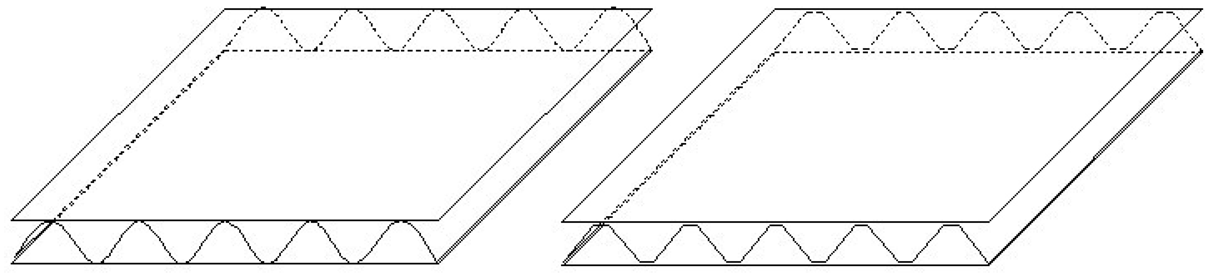
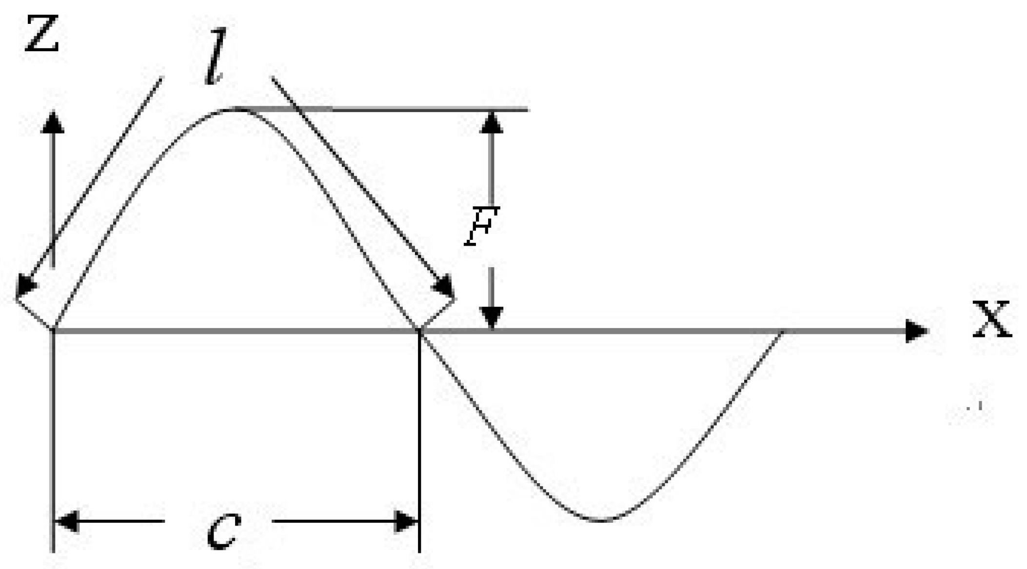
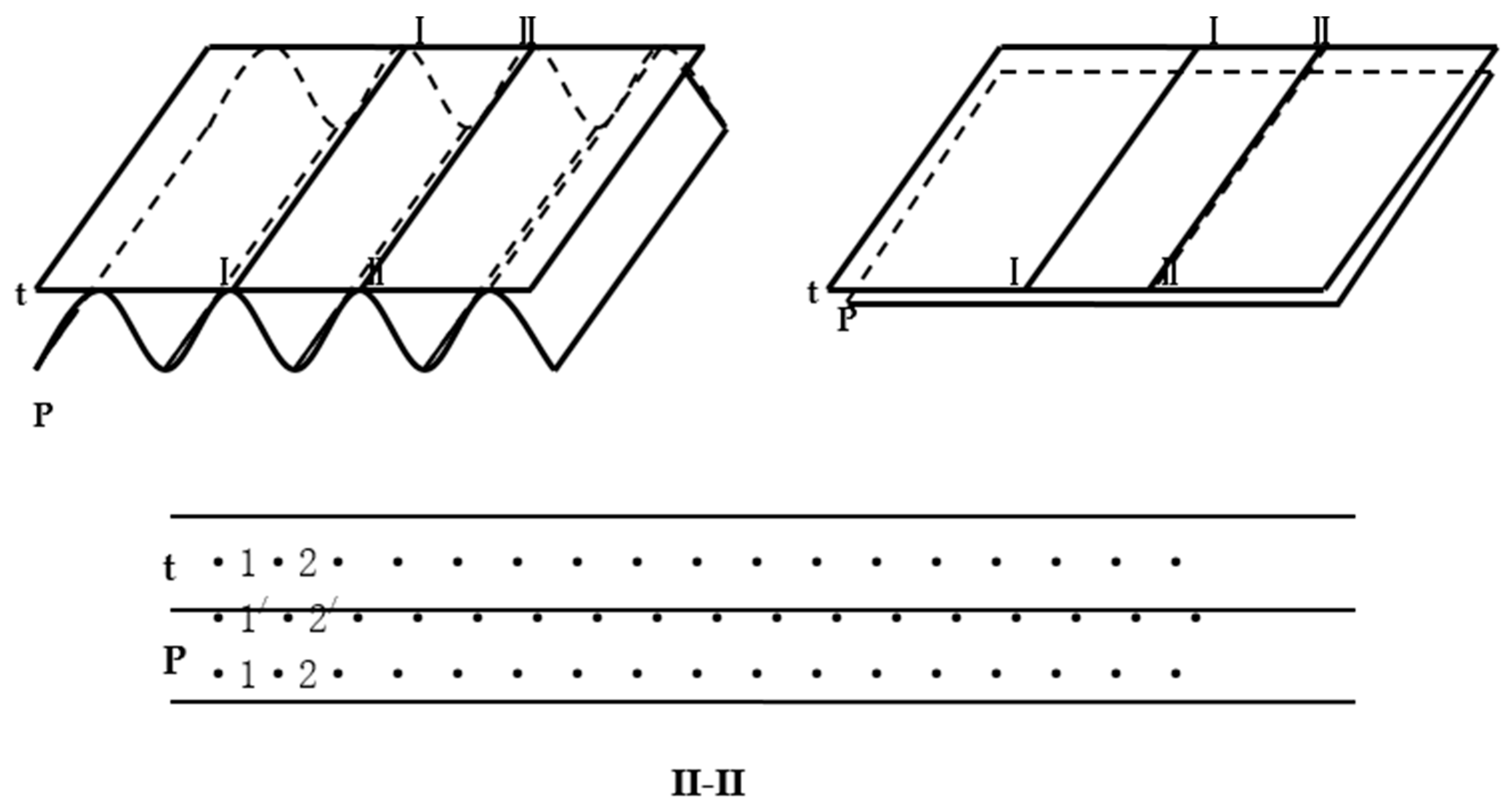
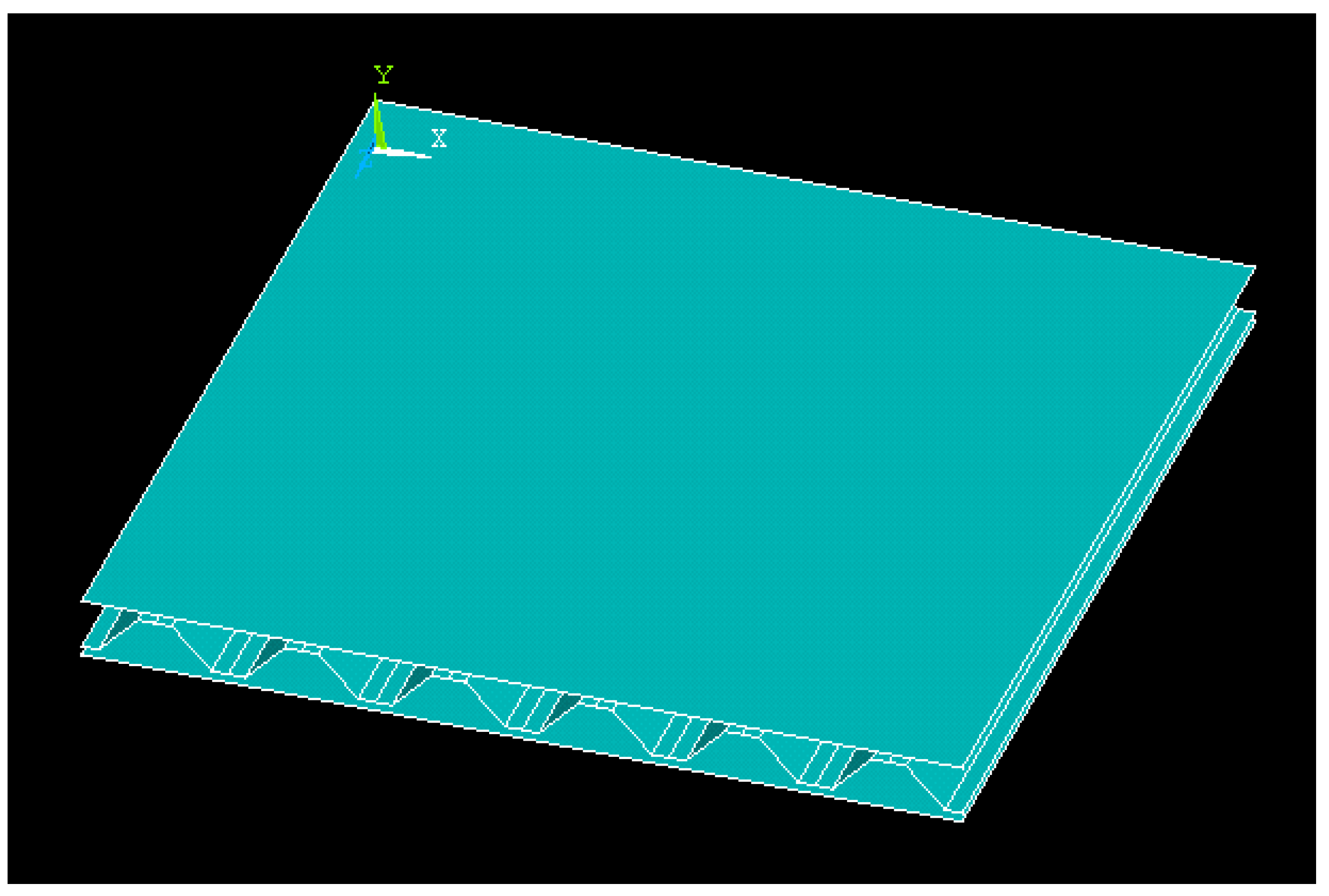
3. Determination of Elastic Constants of the Corrugated Cores

In corrugated sandwich plates, the corrugated core is an important part of the structure used to connect the upper and lower table plates, and the corrugated core is generally in sinusoidal or trapezoidal form (Figure 2). Figure 1 denotes the upper plate by t, the corrugated core by p, and the lower plate by s. In analyzing this sandwich structure, it is necessary to establish its computational model.
Considering the periodicity of the corrugated plate and the fact that it exhibits different elastic properties in the two directions, the corrugated plate can be modeled by comparing it to a homogeneous orthotropic various anisotropic plate. Assuming Young’s modulus as E and Poisson’s ratio as μ, as shown in Figure 3, the elastic constants of the orthotropic plates in the two directions are E x , E y , μ x , μ y , and G . Here, E y = E and μ y = μ . E x , μ x can be solved experimentally and analytically.
Physical equations for the equivalent orthotropic plate are obtained from the generalized Hooke law as follows:
σ x σ y τ x y = 1 ( 1 μ x μ y ) E x E μ 0 E μ E y 0 0 0 ( 1 μ x μ y ) ε x ε y γ x y τ x z τ y z = G x z 0 0 G y z γ x z γ y z
E μ = μ y E x = μ E x
The physical equations of orthotropic plates can be obtained by making E x = E y = E and μ x = μ y = μ in the above equation.
Ref. [19] used orthotropic various anisotropic plates of equal thickness to the corrugated plate for fitting and obtained elastic constants that could more accurately reflect the structural mechanical properties of corrugated plates.
<1>.
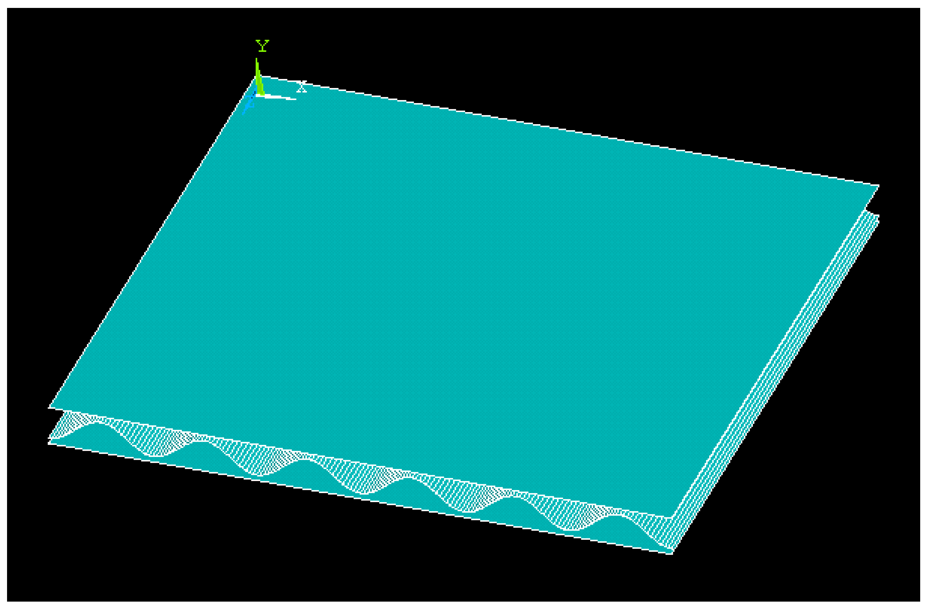
Sinusoidally corrugated core
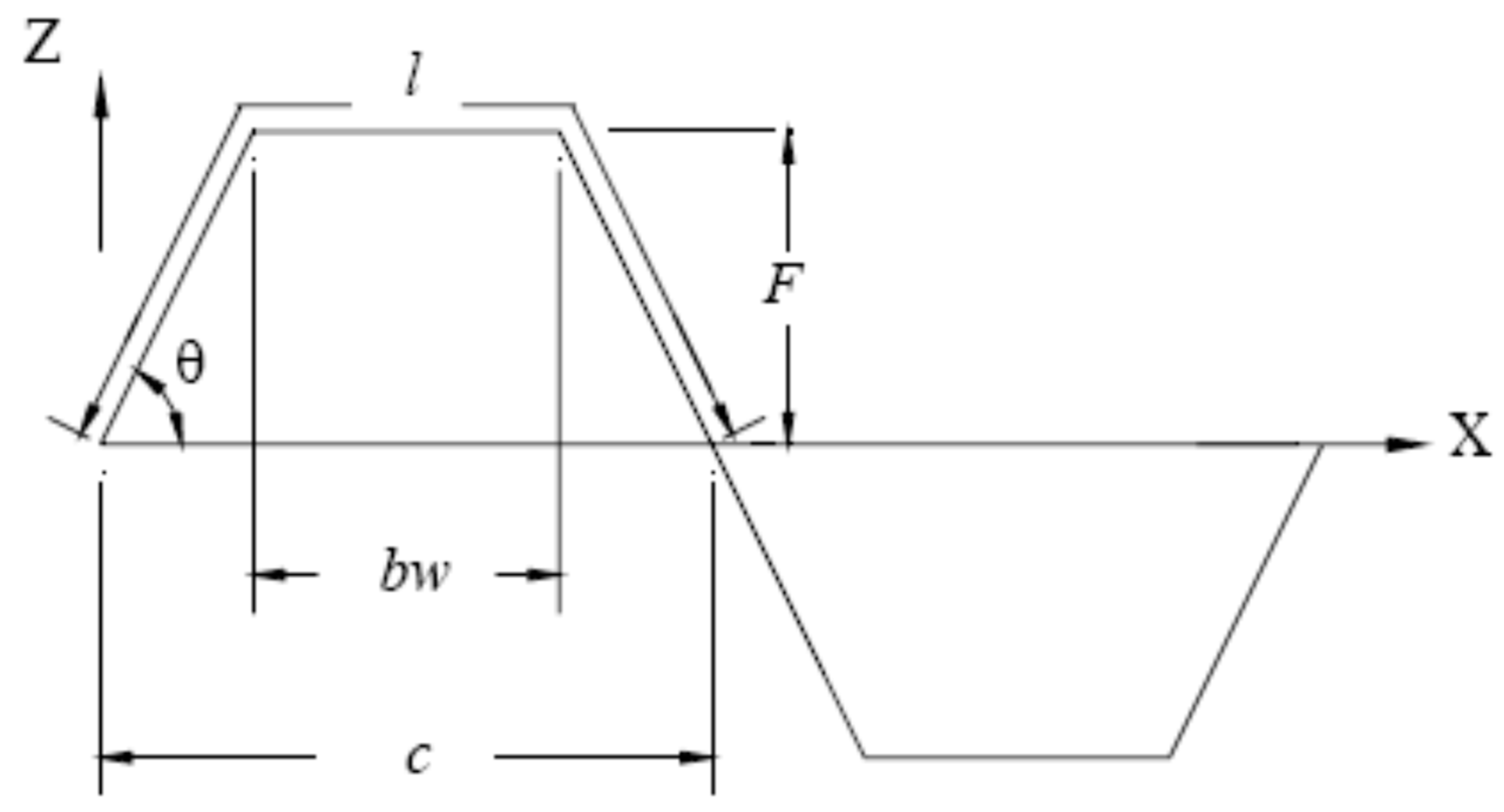
μ y = μ μ x = c l 1 + 6 ( 1 μ 2 ) F h p 2 μ E x = E 1 μ x μ y c l 1 μ 2 E y = μ y μ x E x
<2>.
Trapezoidal corrugated core
μ y = μ μ x = c 2 h p 2 c l h p 2 + 12 α ( 1 μ 2 ) μ α = F 3 3 tan θ + F 2 b w + 1 3 tan 2 θ ( c 3 ( b w + F / tan θ ) 3 )        ( 2 F + b w tan θ ) tan θ ( c 2 ( b w + F / tan θ ) 2 )        + ( 2 F + b w tan θ ) 2 ( c b w + F / tan θ )
The geometric parameters of the corrugated plate c , l , F , b w , and θ are shown in Figure 4 and Figure 5.

4. Meshless Control Equations for Geometric Nonlinearities in Corrugated Sandwich Plates

4.1. Displacement Field Function

According to the mesh-free Galerkin method and the first shear deformation theory (FSDT) [24], the displacements of the orthotropic plate can be approximated by
u ( x , y , z ) = I = 1 n N I ( x , y ) u 0 I ( x , y ) z I = 1 n N I ( x , y ) φ x I ( x , y ) v ( x , y , z ) = I = 1 n N I ( x , y ) v 0 I ( x , y ) z I = 1 n N I ( x , y ) φ y I ( x , y ) w ( x , y ) = I = 1 n N I ( x , y ) w I ( x , y )
The matrix form is expressed as
U = u v w = I = 1 n N I ( x , y ) 0 0 z N I ( x , y ) 0 0 N I ( x , y ) 0 0 z N I ( x , y ) 0 0 N I ( x , y ) 0 0 u o I v 0 I w I φ x I φ y I
where δ I = u 0 I v 0 I w I φ x I φ y I T is the node parameter of the Ith node on the board, n is the number of nodes on the board, and w and φ x , φ y are independent of each other.

4.2. Plate Stress and Strain

4.2.1. Linear Strain

According to von Karmen’s theory of large deflection and FSDT, the strain of the corrugated plate is
ε p = ε x ε y γ x y γ x z γ y z = ε x 0 ε y 0 γ x y 0 0 0 + z ε x 1 z ε y 1 z γ x y 1 γ x z 1 γ y z 1 + ε x L ε y L γ x y L 0 0
ε p = ε x 0 ε y 0 γ x y 0 0 0 0 0 0 + 0 0 0 ε x 1 ε y 1 γ x y 1 γ x z 1 γ y z 1 + ε x L ε y L γ x y L 0 0 0 0 0
where the linear component of the strain includes
ε 0 = ε x 0 ε y 0 γ x y 0 = u 0 x v 0 y u 0 y + v 0 x = I = 1 n B b I 0 δ I
B b I 0 = N I , x 0 0 0 0 0 N I , y 0 0 0 N I , y N I , x 0 0 0
the bending strain is
ε 1 = ε x 1 ε y 1 γ x y 1 = z φ x x z φ y y z ( φ x y + φ y x ) = I = 1 n z B b I b δ I
B b I b = 0 0 0 N I , x 0 0 0 0 0 N I , y 0 0 0 N I , y N I , x
and the shear strain is
γ s = γ x z 1 γ y z 1 = w x φ x w y φ y = I = 1 n B s I δ I
B s I = 0 0 N I , x N I 0 0 0 N I , y 0 N I

4.2.2. Nonlinear Strain

The nonlinear part of the strain after moving the least-square approximation discretization
ε L = ε x L ε y L γ x y L = 1 2 ( w x ) 2 1 2 ( w y ) 2 w y w x = 1 2 w x 0 0 w y w y w x w x w y = 1 2 C I = 1 n G I δ I
C = w x 0 w y 0 w y w x T
G I = 0 0 N I , x 0 0 0 0 N I , y 0 0
The stress in corrugated sheets
σ p = σ x 0 σ y 0 σ x y 0 0 0 0 0 0 + 0 0 0 σ x 1 σ y 1 σ x y 1 σ x z 1 σ y z 1 + σ x L σ y L σ x y L 0 0 0 0 0
The physical equation for a corrugated plate is
σ p = D P ε P
D p = D e 0 0 0 D b 0 0 0 D s
D e = 1 ( 1 μ x μ y ) E x E μ 0 E μ E y 0 0 0 ( 1 μ x μ y ) G x y
D b = 1 ( 1 μ x μ y ) E x E μ 0 E μ E y 0 0 0 ( 1 μ x μ y ) G x y
D s = G x z 0 0 G y z
Above are the stresses and strains for each orthotropic plate, where E μ = μ y E x = μ E x ; for the orthotropic plate, it is sufficient to make E x = E y = E and μ x = μ y = μ .

4.3. Nonlinear Equilibrium Equations for Corrugated Plates

The strain energy generalization of corrugated plates expressed in terms of displacement increments is
Π = d ε p T σ p d v d δ p T F
where d ε p and d δ p are the imaginary strain and imaginary displacement of the corrugated plate, respectively; F is the vector sum of external forces; and σ p is the stress array.
The vector form of strain is written as the relationship between displacement increment and strain increment as follows:
d ε p = B ¯ d δ p
where B ¯ is a function of the displacement δ I .
Substituting Equation (24) into Equation (23), the nonlinear equilibrium equation of the corrugated plate can be obtained by taking the extremum of the strain energy generalized function
ψ ( δ p ) = B ¯ σ P d v F = 0
where
B ¯ = B 0 + B L
B 0 is a constant matrix
B 0 = B 01 ,   B 02 , , B 0 n
B 0 I = B b I e z B b I b B s I
B L is a nonlinear geometric matrix that is a function of δ p
B L = B L 1 ,   B L 2 , , B L n
B L I = C 0 0 G I
From Equation (25)
d ψ = d B ¯ T σ p d v + B ¯ T d σ p d v
From Equation (22)
d σ p = D p d ε p = D p B ¯ d δ p
From Equation (26)
d B ¯ = d B L
Substituting Equations (32) and (33) into Equation (31) yields
d ψ = d B L T σ p d v + B ¯ T D p B ¯ d v d δ p = d B L T σ p d v + K ¯ d δ p
where
K ¯ = K 0 + K L = B ¯ T D p B ¯ d v
K 0 = B 0 T D p B 0 d v
K L = ( B 0 T D p B L + B L T D p B 0 + B L T D p B L ) d v
K 0 is the linear stiffness matrix for small deflections, and K L is the large deflection stiffness matrix or the initial displacement matrix.
d B L T σ p d v = K σ d δ p = ( G T S G d v ) d δ p
G = G 1 ,   G 2 , , G n
S = N x N x y N x y N y
N x = h p / 2 h p / 2 σ x d z N x y = h p / 2 h p / 2 τ y d z N x y = h p / 2 h p / 2 τ y d z
K σ is a symmetric matrix of stress levels called the initial stress matrix or geometric stiffness matrix.
Then Equation (34) can be written as
d ψ = K T d δ p
K T is the tangent stiffness matrix
K T = K 0 + K L + K σ
Then, Equation (32) can be written as
d σ p = D p ( B 0 + B L ) d δ p
Integrating Equation (41) then yields
σ p = D p ( B 0 + 1 2 B L ) δ p
Substituting Equations (35)–(37) into (17)–(19) yields the nonlinear equilibrium equation for the corrugated plate
ψ = ( B 0 + B L ) T D p ( B 0 + 1 2 B L ) d v δ p F = K S δ p F
K S = B 0 T D p B 0 d v + 1 2 B 0 T D p B L d v + B L T D p B 0 d v + 1 2 B L T D p B L d v
The t-plate and s-plate are isotropic plates, and the above process is repeated for both plates. Its governing equations and tangent stiffness matrix can be obtained by making E x = E y = E , μ x = μ y = μ in the derivation process.
The nonlinear equilibrium equations are
ψ t = K S t δ t F t     ψ s = K S s δ s F s
The tangential stiffness matrix is
K T t = K 0 t + K L t + K σ t     K T s = K 0 s + K L s + K σ s
The resulting nonlinear equilibrium equations are solved using the Newton–Raphson iterative method.

4.4. Boundary Conditions and Displacement Coordination Conditions

4.4.1. Full Transformation Method

Due to the fact that the meshless method is based on the moving least-square approximation, the shape function does not satisfy the Kronecker delta properties ( N I ( x J ) = δ I J ), so the displacement boundary conditions cannot be imposed directly. In this paper, the full transformation method is adopted, using which the node parameters can be effectively converted into the nodes’ actual displacement. This satisfies the Kronecker condition, and the displacement boundary conditions can then be introduced to correctly solve the equations.
In the moving least-square approximation, the node parameters are used as the approximation variables of the approximation function
u i h ( x ) = I = 1 n N I ( x ) u i I
where uiI is the function component of the i-th direction of the I-th node, uiI is the node parameter, NI is the form function of the i-th node, and n is the number of nodes in the problem domain.
We write Equation (46) in matrix form to find
U h = φ U
φ = N 1 ( x 1 ) N 2 ( x 1 ) N n ( x 1 ) N 1 ( x 2 ) N 2 ( x 2 ) N n ( x 2 ) N 1 ( x n ) N 2 ( x n ) N n ( x n )
The relationship between the true displacement and the node parameters can be expressed as follows:
U ¯ U h = φ U
Assuming T = φ 1 , Equation (48) is expressed as
U = T U ¯
Therefore, by substituting Equation (49) into the general governing equations of the meshfree Galerkin method (KU = P), both sides are multiplied by matrix T, and we obtain
T T K T U ¯ = T T P
A new governing equation can be obtained
K ¯ U ¯ = P ¯
where
K ¯ = T T K T
P ¯ = T T P
The equation is solved by taking the real displacement as the unknown quantity, which can satisfy the displacement boundary condition, and thus the equation can be solved.

4.4.2. Treatment of Boundary Conditions

The same full transformation method can be used to deal with the nonlinear equilibrium equations, using Equation (49) to represent the node parameters in terms of the nodes’ actual displacement. Substituting δ = H δ ¯ and d δ = H d δ ¯ into Equations (39) and (43) to displace and then orthogonalize gives
d H T ψ = H T K T H d δ ¯
H T ψ = H T K S H δ ¯ H T F
We can find
ψ ¯ = H T ψ ,   K ¯ T = H T K T H ,   F ¯ = H T F ,   K ¯ S = H T K S H
Then, Equation (54) and Equation (55) can be rewritten as
d ψ ¯ = K ¯ T d δ ¯
ψ ¯ = K ¯ S δ ¯ F ¯
In this way, the unknown quantity can be expressed as the node displacement, and the meshless Galerkin nonlinear equilibrium equation at this time can directly impose the displacement boundary condition.
Since the corrugated sandwich plate is a composite laminate structure combined by three plates, the coupling problem between its plates needs to be studied. Taking the sinusoidal corrugated sandwich plate as an example, as shown in Figure 6, there must be equal displacement vectors at its intersection line.
Taking the upper surface plate t-plate and the corrugated plate p-plate as an example, the displacements on the cross-section II-II of the junction line should satisfy the following relationship:
w ¯ t = w ¯ 1 = w ¯ p φ x ¯ t = φ x ¯ 1 = φ x ¯ p φ y ¯ t = φ y ¯ 1 = φ y ¯ p
where “t” denotes the physical quantity of the upper surface plate, “p” denotes the physical quantity of the corrugated plate, and “l ” denotes the physical quantity on the boundary line. Assuming that each plate is discretized with m nodes and that there are n nodes on the intersection line, Equation (59) can be written in the following matrix form:
δ ¯ t = Λ δ ¯ p
δ ¯ t = w 1 ¯ t , φ x 1 ¯ t , φ y 1 ¯ t , , w n ¯ t , φ x n ¯ t , φ y n ¯ t
δ ¯ p = w 1 ¯ p , φ x 1 ¯ p , φ y 1 ¯ p , , w n ¯ p , φ x n ¯ p , φ y n ¯ p
Λ is a unit matrix of order 3n × 3n.
After the full transformation process, the displacement boundary conditions are introduced into the equilibrium equations for the upper surface plate t and the lower surface plate s. The stiffness matrix and the corresponding displacements are primitively transformed. After extracting the terms related to the degrees of freedom A and B from the 5 degrees of freedom of the node on the intersection line and putting them together, we obtain
ψ ¯ i t ψ ¯ l t = K ¯ s i i t K ¯ s i l t K ¯ s l i t K ¯ s l l t δ ¯ i t δ ¯ l t F ¯ i t F ¯ l t ψ ¯ l s ψ ¯ i s = K ¯ s l l s K ¯ s l i s K ¯ s i l s K ¯ s i i s δ ¯ l s δ ¯ i s F ¯ l s F ¯ i s
with tangential stiffness as
K ¯ T t = K ¯ T i i t K ¯ T i l t K ¯ T l i t K ¯ T l l t K ¯ T s = K ¯ T i i s K ¯ T i l s K ¯ T l i s K ¯ T l l s
where δ ¯ l denotes the displacement vector of the nodes of order 3n at the intersection line between the plates, and δ ¯ i denotes the displacement vector of the nodes of order 5m − 3n within the plate excluding the nodes at the intersection line. Moreover, K ¯ s i i is the stiffness matrix of order 5m − 3n × 5m − 3n, K ¯ s l l is the stiffness matrix of order 3n × 3n, K ¯ s i l is the stiffness matrix of order 5m − 3n × 3n, and K ¯ s l i is the stiffness matrix of order 3n × 5m − 3n, and the same method of chunking is used for ψ ¯ and F ¯ .
The corrugated p-plate is in contact with both the t- and s-plates and is therefore represented in block form as
ψ ¯ l ( 1 ) ψ ¯ i ( 1 ) ψ ¯ l ( 2 ) = K ¯ s l l ( 11 ) K ¯ s l i ( 11 ) K ¯ s l l ( 12 ) K ¯ s i l ( 11 ) K ¯ s i i ( 11 ) K ¯ s i l ( 11 ) K ¯ s l l ( 21 ) K ¯ s l i ( 21 ) K ¯ s l l ( 22 ) δ ¯ l ( 1 ) δ ¯ i ( 1 ) δ ¯ l ( 2 ) F ¯ l ( 1 ) F ¯ i ( 1 ) F ¯ l ( 2 )
K T P = K ¯ T l l ( 11 ) K ¯ T l i ( 11 ) K ¯ T l l ( 12 ) K ¯ T i l ( 11 ) K ¯ T i i ( 11 ) K ¯ T i l ( 11 ) K ¯ T l l ( 21 ) K ¯ T l i ( 21 ) K ¯ T l l ( 22 )
The stiffness matrices are first superimposed, at which point the displacement coordination condition needs to be met, i.e., δ ¯ l ( 1 ) = δ ¯ l t , δ ¯ l ( 2 ) = δ ¯ l s . The overall stiffness matrix of the integrated corrugated sandwich plate, with each plate viewed as an independent unit, is
K ¯ S G = K ¯ s i i t K ¯ s i l t 0 0 0 K ¯ s l i t K ¯ s l l t + K ¯ s l l ( 11 ) K ¯ s l i ( 11 ) K ¯ s l l ( 12 ) 0 0 K ¯ s i l ( 11 ) K ¯ s i i ( 11 ) K ¯ s i l ( 11 ) 0 0 K ¯ s l l ( 21 ) K ¯ s l i ( 21 ) K ¯ s l l ( 22 ) + K ¯ s l l s K ¯ s l i s 0 0 0 K ¯ s i l s K ¯ s i i s
K ¯ T G = K ¯ T i i t K ¯ T i l t 0 0 0 K ¯ T l i t K ¯ T l l t + K ¯ T l l ( 11 ) K ¯ T l i ( 11 ) K ¯ T l l ( 12 ) 0 0 K ¯ T i l ( 11 ) K ¯ T i i ( 11 ) K ¯ T i l ( 11 ) 0 0 K ¯ T l l ( 21 ) K ¯ T l i ( 21 ) K ¯ T l l ( 22 ) + K ¯ T l l s K ¯ T l i s 0 0 0 K ¯ T i l s K ¯ T i i s
The integrated nonlinear equilibrium equation is
ψ ¯ G = K ¯ S G δ ¯ G F ¯ G
ψ ¯ G = ψ ¯ i t ψ ¯ l t ψ ¯ i ( 1 ) ψ ¯ l s ψ ¯ i s
δ ¯ G = δ ¯ i t δ ¯ l t δ ¯ i ( 1 ) δ ¯ l s δ ¯ i s
F ¯ G = F ¯ i t F ¯ l t F ¯ i ( 1 ) F ¯ l s F ¯ i s
This approach can be applied to solve the nonlinear surface problem of the corrugated sandwich plate. To ensure accurate coupling, a sufficient number of nodes must be distributed along the interface.
When the core consists of a trapezoidal corrugated plate, the junction along the centerline of the interface is selected as the coupling point. The computational model of the composite structure is then established using the same coupling method as that of the sinusoidal.

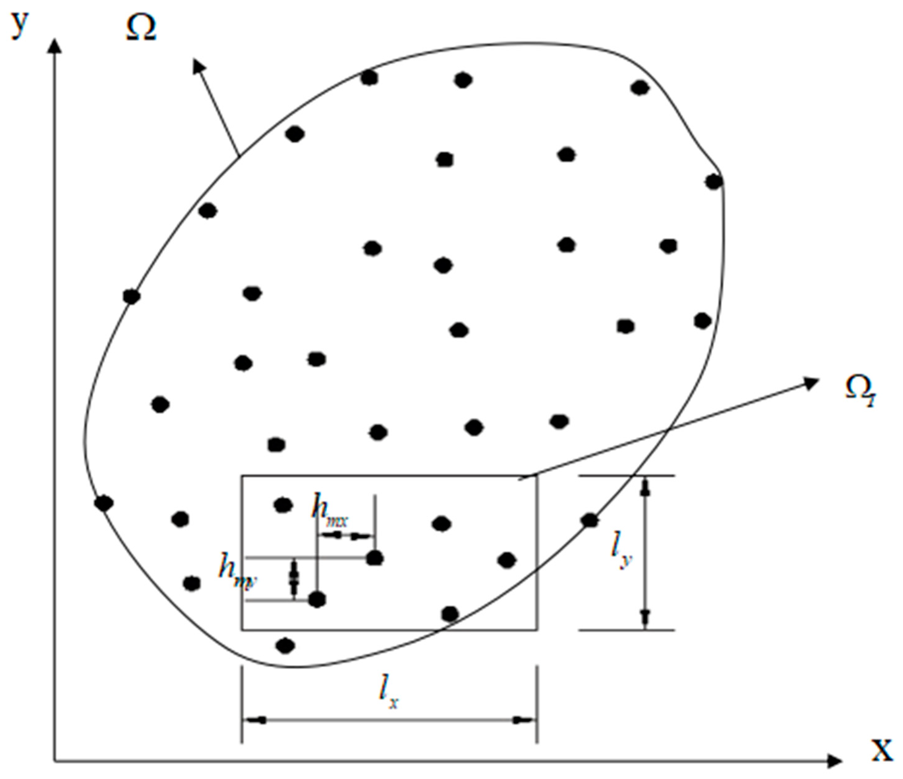
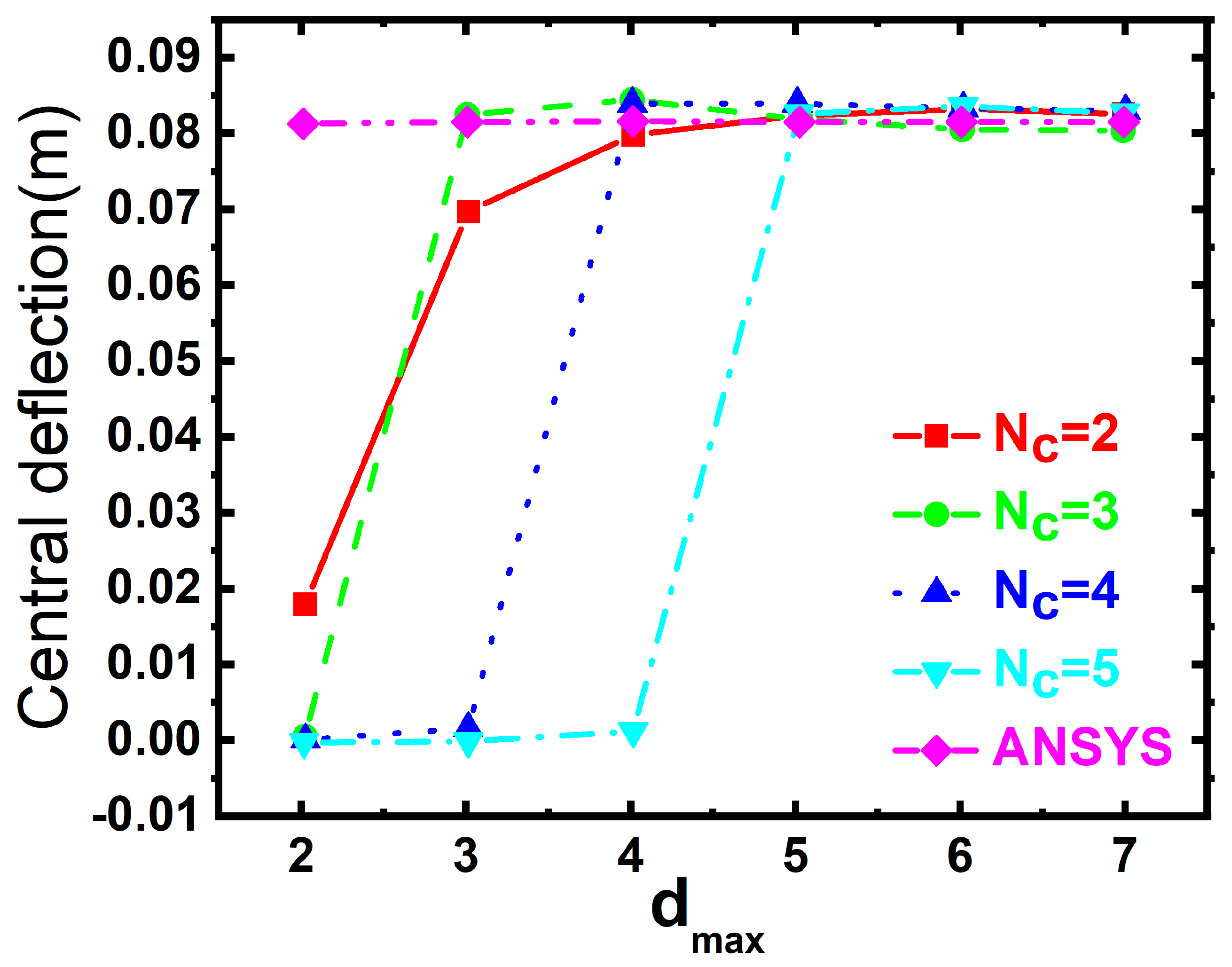
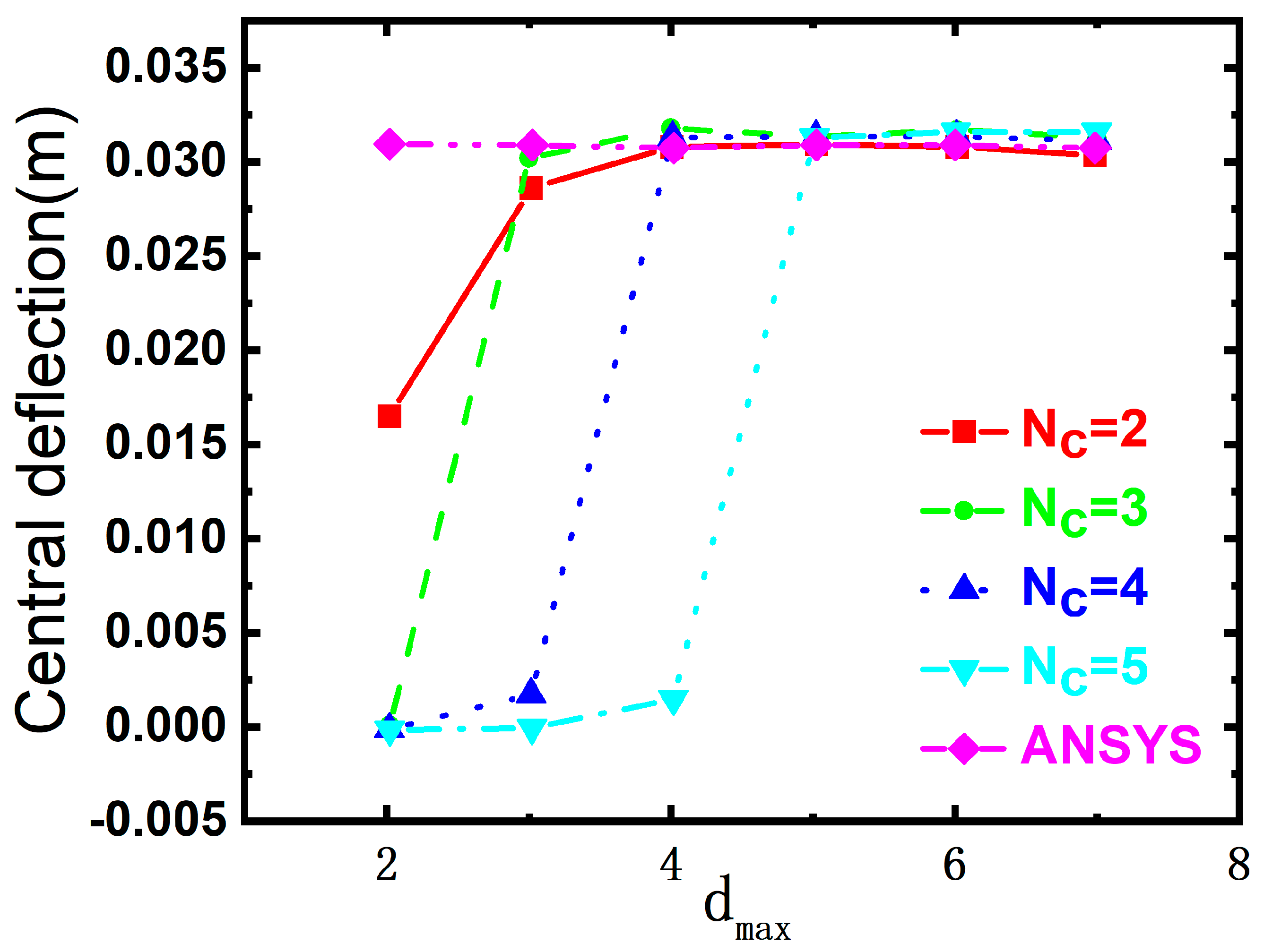
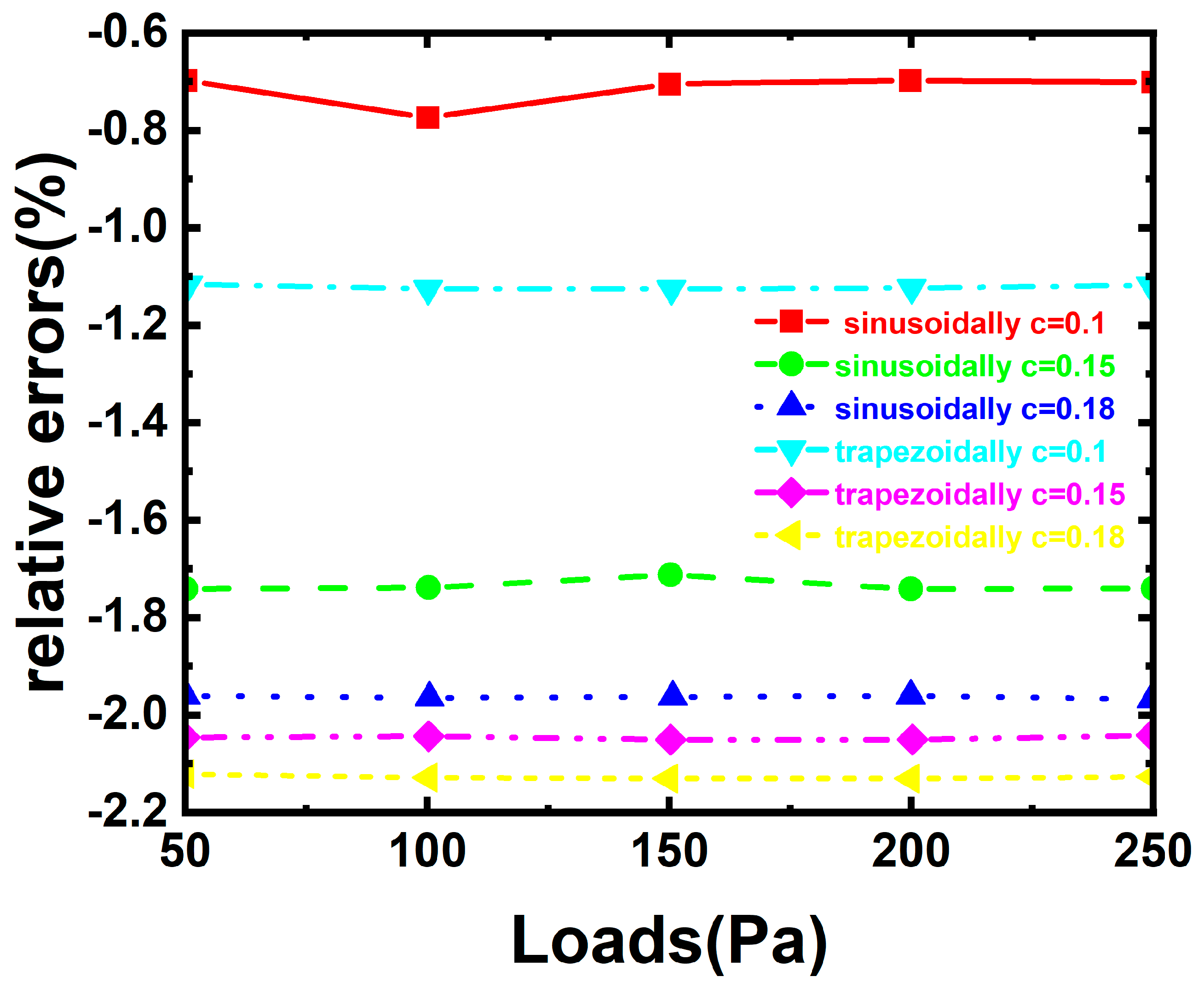
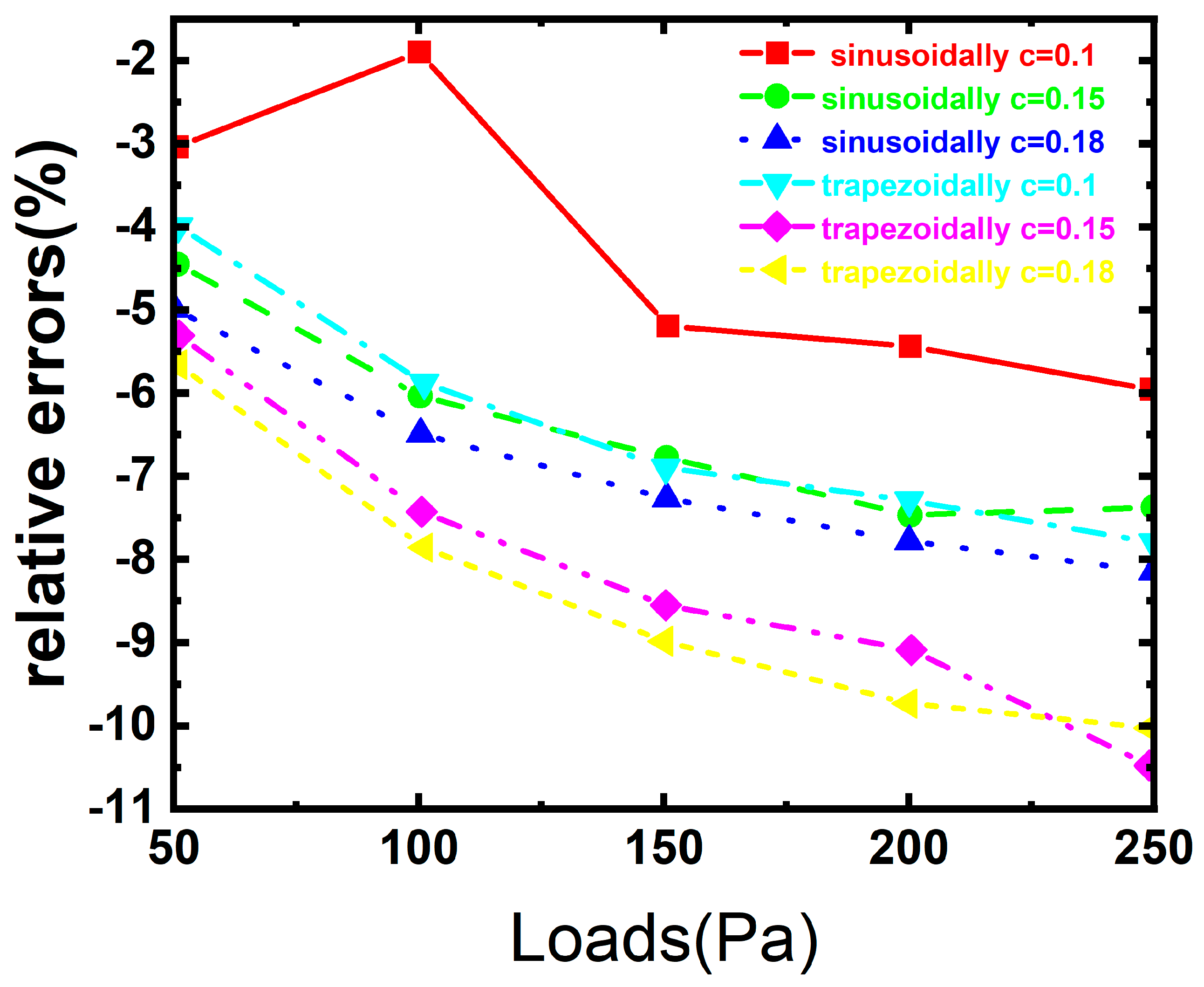
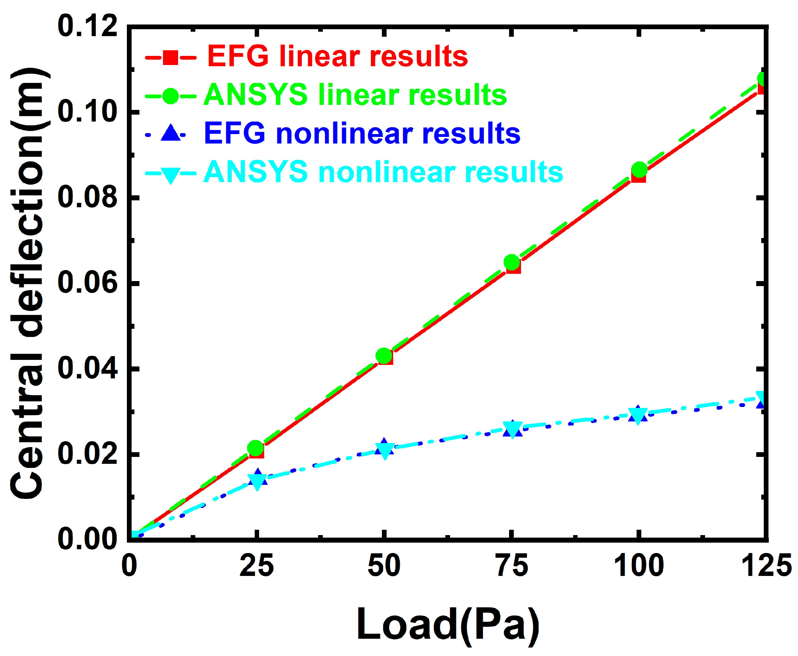
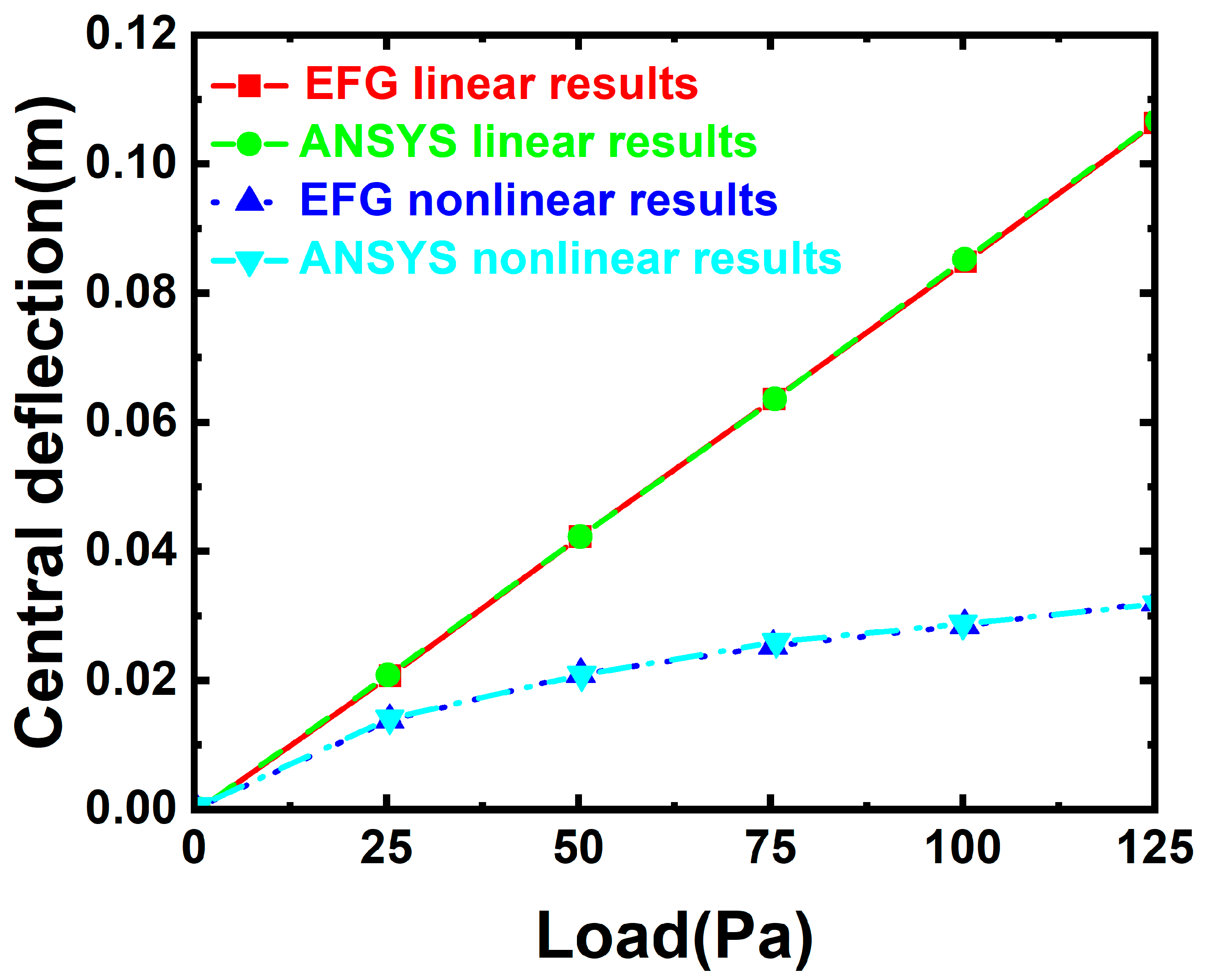
5. Results and Discussion

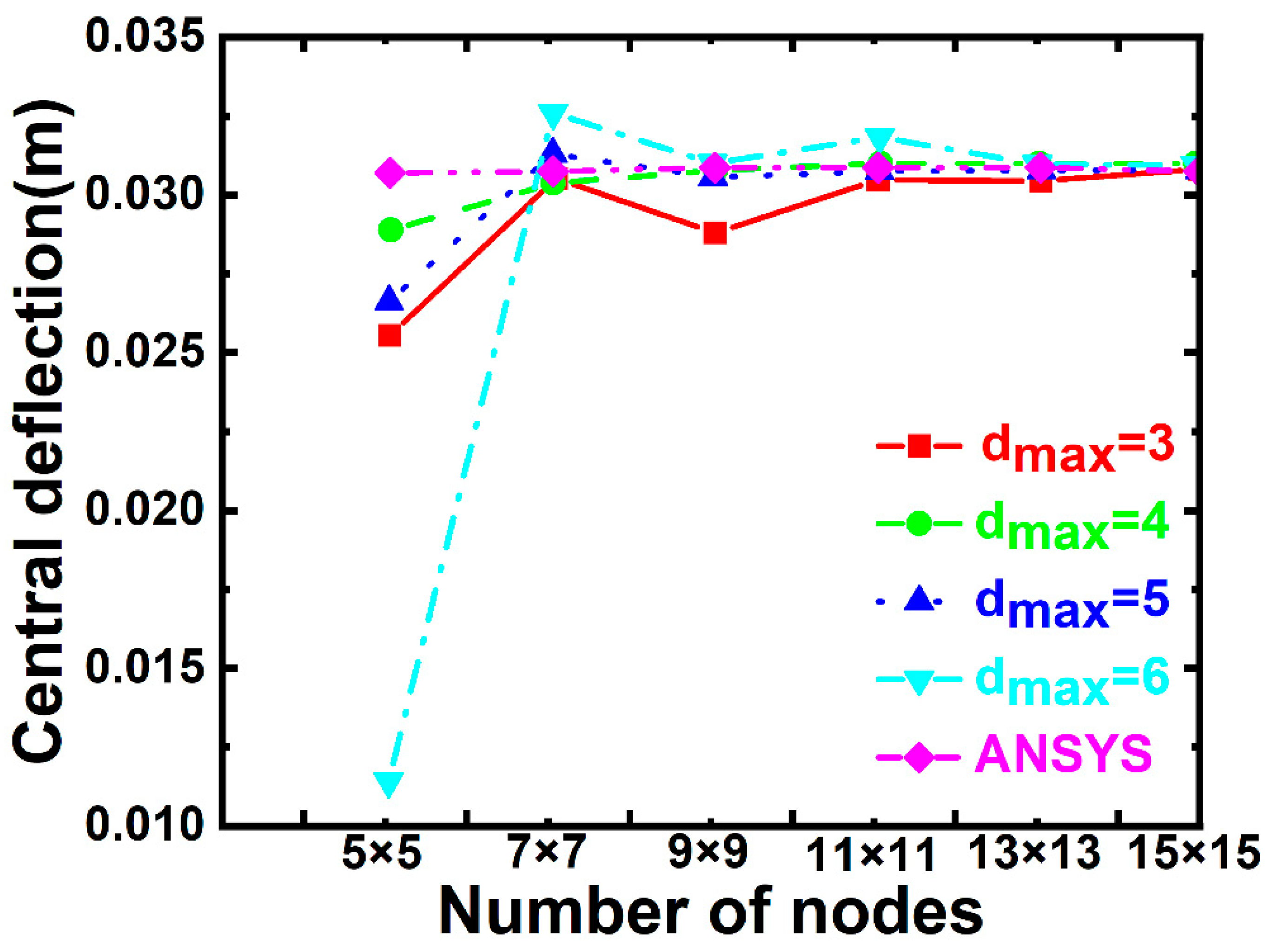
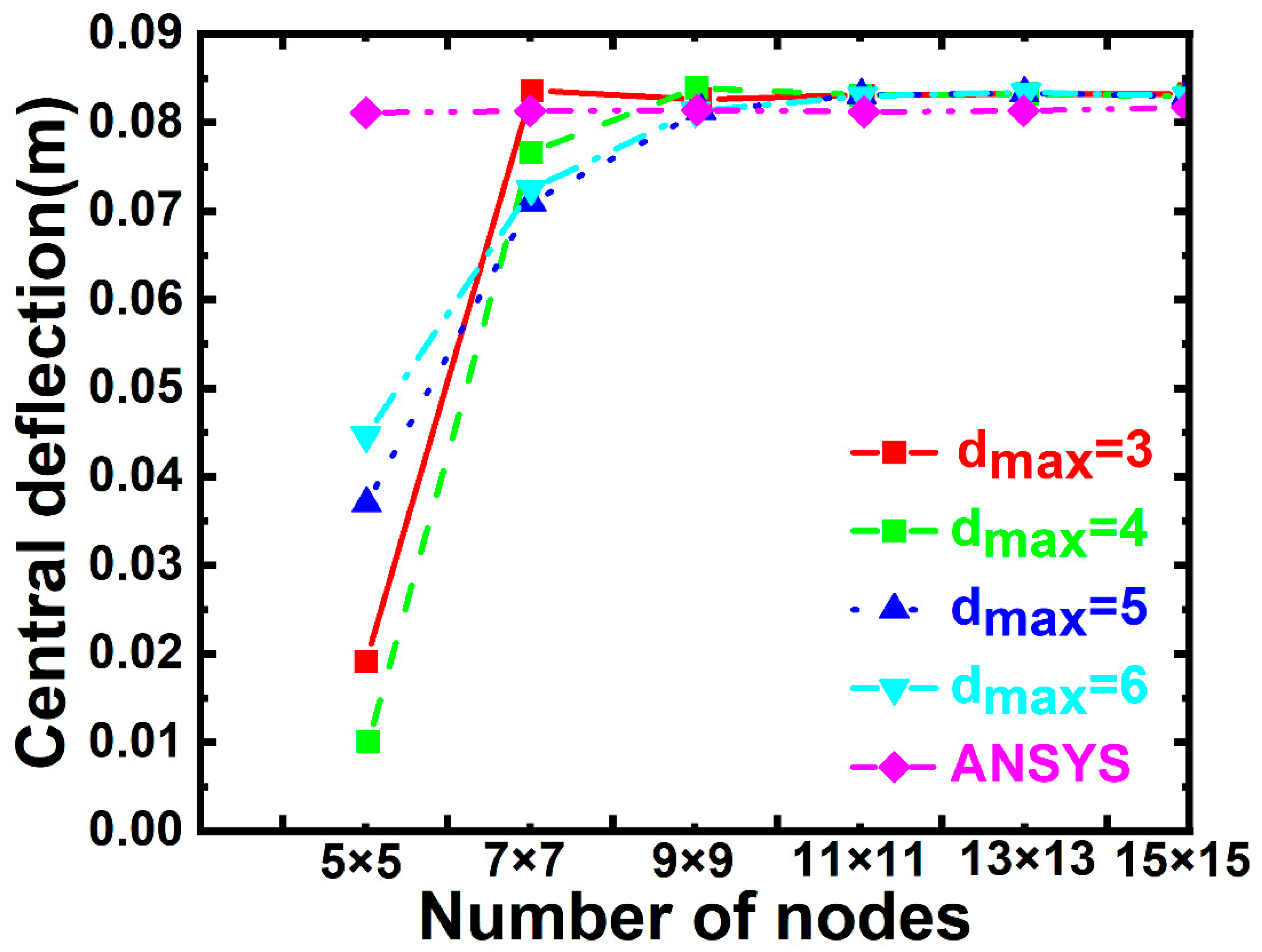
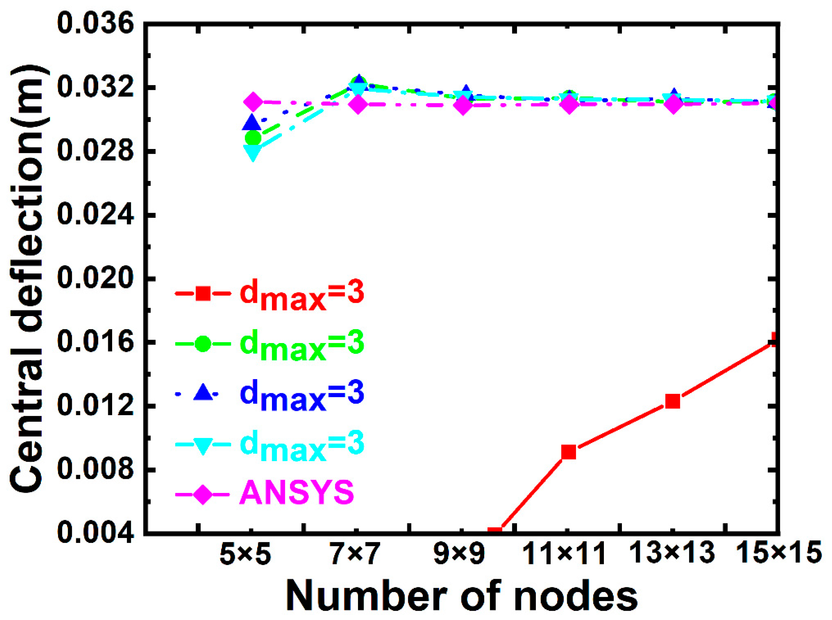
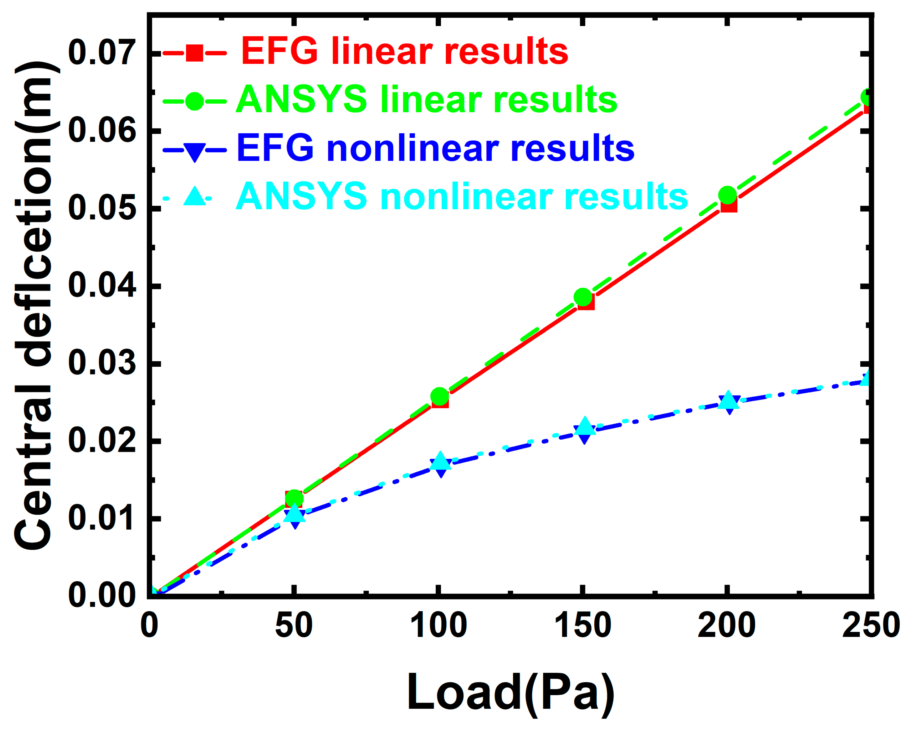
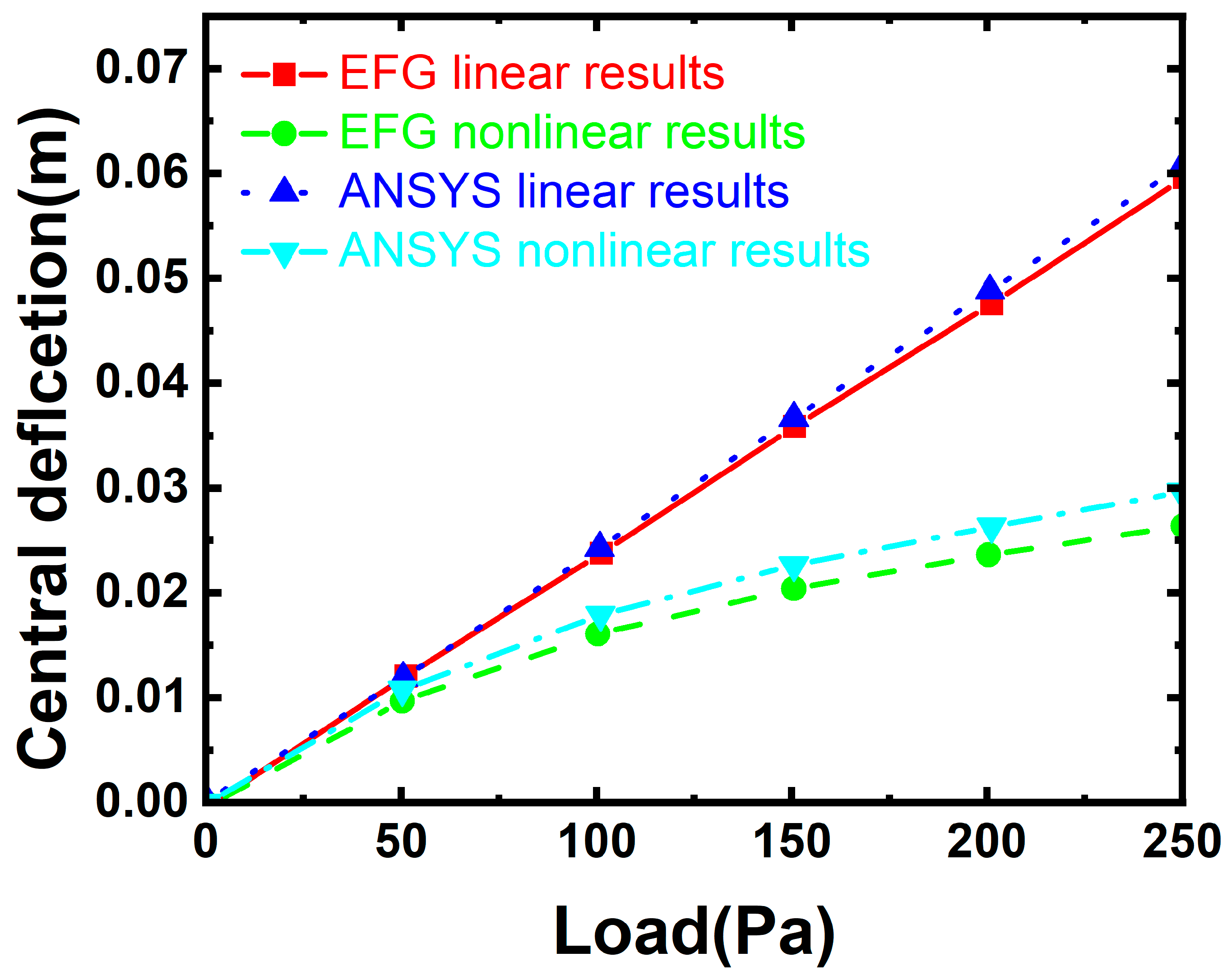
5.1. Validation Studies

An example is used to show the convergence of the proposed method and the effects that the domain of influence of the nodes and the order of the basis functions have on this convergence.
The rectangular domain of influence is used in this study. Rectangular support is employed, and thus the scaling factors d max x and d max y are defined as:.
d max x = l x h m x ,   d max y = l y h m y
Here (Figure 7), l x and l y are the lengths of the rectangular support in the x and y directions, respectively, and h m x and h m y are the distances between two neighboring nodes in the x and y directions, respectively. For convenience, we choose d max = d max x = d max y .
In this paper, a square flat plate is taken as an example, for which the side length is L = W = 1.8 m, the plate thickness is h = 0.18 m, and the modulus of elasticity is E = 3 × 10⁷ Pa, with a Poisson’s ratio μ = 0.3 . In this paper, the meshless Galerkin method is discretized with uniform nodes and the distribution density is 9 × 9 nodes to calculate and analyze the linear and nonlinear bending of the flat plate. The calculated results after simulation with ANSYS finite element software are compared with the method of this paper, using solid45 and shell63 elements simulation. The convergence of the computational results of the four-sided solidly supported flat plate with respect to the basis function order N c and the influence domain system d max is given in Figure 8.
Figure 8 and Figure 9 depict the relationship between the convergence of this method and the order of the basis function and the size of the domain of influence. When the distribution density of the nodes is certain, the results of using the basis function of order N c = 2 to N c = 5 can converge when the coefficient of the domain of influence is d max ≥ 5, and the higher the order, the larger the domain of influence needs to be in order to converge; at the same time, the computation is time-consuming and the larger the consumption of the computation is.
The following discusses the change in convergence of this method with the size of the influence domain and the density of the node distribution when the basis functions are taken from the second to the fifth order, respectively. The above model is also used, and the boundary is a four-sided solid support.
As can be seen in Figure 10, Figure 11, Figure 12, Figure 13, Figure 14 and Figure 15, the results are easy to converge as the domain of influence increases and fewer nodes are required, but for the N = 4th order basis functions, the domain of influence is too small and it is difficult to converge, and the distribution of required nodes is also greater.
It is clear from the above analysis and study that the computational accuracy will not be greatly improved by the improvement of the order of the basis function, and the computational efficiency will be affected by too high an order instead. The larger the domain of influence, the more accurate the results obtained, and the greater the computational cost and loss. From the above graphs, it can be seen that when the basis function is of order N c = 2 and the domain of influence takes the coefficient of d max = 4 , the convergence of the results obtained and the computational accuracy are satisfactory.

5.2. Four-Side Fixed Support Corrugated Sandwich Plate

Example 1.
Sinusoidal Corrugated core sandwich square plate with side length L = 1.8 m, W = 1.8 m, thickness of all three plates h = 0.018 m, corrugated core geometrical parameter c = 0.15 m, F = 0.006 m, modulus of elasticity E = 3 × 10⁷ Pa, Poisson’s ratio  μ = 0.3 , P taken to be from 50 to 250 Pa, and 6 complete waveforms. The large deflection problem of the structure is analyzed by the meshless Galerkin method, and the nodes are arranged as 3 × 13 × 13 with a total of 507 nodes.
(1) ANSYS simulation using shell181 elements, with a total of 10,317 discrete nodes (Figure 16), and the results of the two methods are compared, as shown in Table 1 and Figure 17 below.
(2) For the sinusoidal corrugated sandwich plate, ANSYS simulation is performed using shell181 elements, the corrugated plate is fitted with orthotropic plates with a total of 507 discrete nodes, and the results of the simulation are compared with the results calculated by the methodology of this paper, as shown in Table 2 and Figure 18 below.
Example 2.
Trapezoidal form corrugated core sandwich square plate with side length L = 1.8 m, W = 1.8 m, three plates with thicknesses h = 0.018 m, corrugated core geometrical parameters c = 0.15, F = 0.006 m, modulus of elasticity E = 3 × 10⁷ Pa, Poisson’s ratio  μ = 0.3 , P taken as 50–250 Pa, and 6 complete waveforms. The large deflection problem of the structure is analyzed by the meshless Galerkin method, and the nodes are arranged as 3 × 13 × 13 with a total of 507 nodes.
(1) ANSYS simulation is performed using shell181 elements, with a total of 20,729 discrete nodes(Figure 19), and the results of the calculations of the two methods are compared, as shown in Table 3 and Figure 20 below.
(2) For the trapezoidal corrugated sandwich plate, ANSYS simulation is performed using shell181 elements, the corrugated plate is fitted with orthotropic plates with a total of 507 discrete nodes, and the simulation results are compared with the calculation results of the method in this paper, as shown in Table 4 and Figure 21 below.
Example 1 and Example 2 show that the method used in this paper can achieve the results that satisfy the accuracy by using very few node discretizations, and the accuracy of the method of used in paper can be seen from the linear solution. When the plate is subjected to a load of more than 50 Pa, a more serious nonlinear phenomenon occurs with the increase in plate deflection; at this time, instead of continuing to apply the linear solution, as it is prone to large errors, it is appropriate to refer to the nonlinear solution. The finite element processing of nonlinear problems may appear as mesh distortion problems, and the larger the load generated by the larger deflection, the higher the likelihood of the occurrence of the above problems, so relative to the linear solution, the nonlinear solution’s error is larger, but within the scope of the engineering-allowable meshless method, the denser the nodes used, the more accurate the results obtained will be. When ANSYS finite element simulation was applied for a corrugated plate, that is, the corrugated plate was compared to an orthotropic plate of equal thickness via the method used in this paper and the finite element method using the same corrugated sandwich plate model, the four sides of the solid support results obtained by the comparative analysis of the accuracy of this paper’s method were verified.
Example 3.
Adopting the elastic constants and structural parameters of Example 1, under the action of uniform load P = 100 Pa, the half wavelength of the corrugated plate c = 0.15 m for any of the six complete waveforms, and the half-wave height F of the corrugated plate is taken from 0.004 to 0.04, and then we discuss the applicability of its value to the theory of this paper for solving the geometric nonlinearities of the corrugated sandwich plate. The results obtained are compared with the finite element ANSYS simulation results; the shell181 element is used in this case, which is the same as the above two cases; and the comparison results are shown in Table 5 below.
Example 3 analyzes the half-wave height of the corrugated sandwich plate, and as the half-wave height F increases, the stiffness of the corrugated sandwich plate is enhanced and the resulting deflection becomes smaller; moreover, from the results, it can be seen that the error is too large when F is taken from 0.01 m to 0.02 m, so that it is not suitable for F to be taken as the value of this interval. From an engineering point of view, half-wave heights should be avoided as much as possible by taking values in this range.
Example 4.
Using the elastic constants of Example 1 and Example 2, the length of the corrugated side L = 1.8 m, the straight side W = 1.8 m, the loss height of the corrugated plate F = 0.006 m, and the trapezoidally corrugated sandwich plate  θ = 45 , respectively, under the action of homogeneous load P = 50–250 Pa highlight the value of the half-wavelength of the corrugated plate, c, and the applicability of this paper’s theory for solving the geometric nonlinear problem of the corrugated sandwich plate. Two different forms of corrugated sandwich plates are analyzed, i.e., sinusoidal and trapezoidal corrugated sandwich plates. The results obtained are compared with the finite element ANSYS simulation results; in this case, the shell181 unit is used, which is the same as the above two examples; the comparison results are shown in Figure 22 and Figure 23, and the corrugated sandwich plates and corrugated plate half-wavelength, c, take values of 0.1 m, 0.15 m, and 0.18 m.
Example 4 illustrates that the relative error between the results of this paper’s method and those of the finite element method for a plate of the same length decreases with the increase in the number of corrugations. And as the load increases, the larger the displacement is, the larger the relative error generated. In practice, the increase in the number of corrugations makes the support effect of the corrugated plate core on the side plate more obvious, the strength of the corrugated plate is also improved, the mechanical properties are closer to the orthotropic anisotropic plate that the method used in this paper approximates with, and the accuracy of the calculation is improved.

5.3. Four-Side Simply Supported Corrugated Sandwich Plates

Example 5: Trapezoidal corrugated core sandwich square plate with side length L = 1.8 m, W = 1.8 m, thickness of all three plates h = 0.018 m, corrugated core geometrical parameter c = 0.15 m, F = 0.004 m, modulus of elasticity E = 3 × 10⁷ Pa, Poisson’s ratio μ = 0.3 , trapezoidal corrugated core sandwich plate θ = 45 , P taken as the value of 25~125 Pa, and six complete waveforms. The large deflection problem of the structure is analyzed by the meshless Galerkin method, and the nodes are arranged as 3 × 13 × 13 with a total of 507 nodes.
(1) ANSYS simulation using shell181 elements, with a total of 10,317 discrete nodes, and the simulation results and the calculation results of the method used in this paper are compared, as shown in Table 6 and Figure 24 below.
(2) The ANSYS simulation uses shell181 elements, the corrugated plate is fitted with orthotropic plates with a total of 507 discrete junctions, and the results of the two methods are compared, as shown in Table 7 and Figure 25 below.
Example 6: A sinusoidal corrugated sandwich square plate with side length L = 1.8 m, three plates with thicknesses h = 0.018 m, corrugated core geometric parameters c = 0.15 m, F = 0.006 m, modulus of elasticity E = 3 × 10⁷ Pa, Poisson’s ratio μ = 0.3 , P taking the value of 50 Pa, six complete waveforms, and W taking the value of 1.5 m–5.1 m or 5.4 m, discussing the applicability of their values to the theory of this paper for solving the geometrical nonlinearities of the corrugated sandwich plate. The applicability of these values for solving the geometric nonlinearity problem of corrugated sandwich plates is discussed. The obtained results are compared with the finite element ANSYS simulation results; in this case, the shell181 unit is used, and the comparison results are shown in Table 8 below.
In Example 5 and Example 6, when the half-wave height F is less than 0.01 and the boundary condition is four-sided simply supported, the results obtained using the proposed method for the corrugated sandwich plate model show good agreement with the ANSYS finite element simulation results. The method presented in this paper effectively analyzes the nonlinear behavior of the corrugated plate model. When the boundary conditions are four-sided simply supported and the aspect ratio W/L ranges from 1.5 to 3.0, the relative error between the proposed method and the ANSYS finite element simulation results tends to stabilize. When the aspect ratio is in this range, it has less effect on shear deformation and is more suitable for simulation applications in engineering. In the ANSYS finite element simulation of the corrugated plate, the same modeling approach as in this paper is adopted—approximating the corrugated plate as an orthotropic plate of equivalent thickness. A comparative analysis of the results obtained using both methods under four-sided simply supported conditions confirms the accuracy and reliability of the proposed approach.

6. Conclusions

In this study, a meshless model for analyzing the nonlinear behavior of corrugated sandwich plate structures has been developed from the perspective of composite structures. To simplify the complex geometry while ensuring accuracy, the corrugated core is approximated as an orthotropic anisotropic plate. The displacement field functions for each plate component are constructed based on first-order shear deformation theory (FSDT) and the moving least-square (MLS) approximation. Nonlinear stress and strain expressions are derived using FSDT and von Kármán’s large deflection theory, and the nonlinear equilibrium equations for each plate are formulated via the principle of virtual work. To obtain the governing nonlinear equilibrium equations for the entire corrugated sandwich plate structure, boundary conditions are handled using a full transformation approach, and displacement continuity conditions are enforced. The resulting system of equations is then solved iteratively using the Newton–Raphson method.
Based on the numerical results of the example solution, the following conclusions can be drawn:
(1)
The proposed meshless model achieves high accuracy while requiring significantly fewer computational nodes compared to traditional finite element methods (FEMs) with fine mesh discretization;
(2)
The close agreement between the meshless and FEM solutions confirms the effectiveness and reliability of the proposed approach;
(3)
The method exhibits high computational efficiency and is well suited for numerical implementation, making it a promising tool for analyzing the nonlinear behavior of corrugated sandwich plate structures.
The above conclusions show that the use of the meshless method to establish the meshless Galerkin method model of the geometric nonlinear problem of a corrugated sandwich plate avoids the constraints of the mesh in the finite element method and can carry out accurate calculations for more complex cases. The calculation results are more in line with the actual mechanical behavior of the project, which can effectively refer to the prevention and treatment of large deformation behavior in the application of corrugated sandwich plates and can be more widely used in the fields of aerospace manufacturing, shipbuilding, and civil engineering.

Author Contributions

L.P.: Writing—original draft, Writing—review and editing, Supervision, Project administration. Z.Z.: Writing—original draft, Writing—review and editing, Visualization, Software, Formal analysis. D.W.: Writing—review & editing. P.T.: Writing—review and editing. G.M.: Writing—original draft, Methodology, Investigation, All authors have read and agreed to the published version of the manuscript.

Funding

This research received no external funding.

Data Availability Statement

Data will be made available on request.

Conflicts of Interest

The authors declare that they have no known competing financial interests or personal relationships that could have appeared to influence the work reported in this paper.

References

  1. Reissner, E. On bending of elastic plates. Q. Appl. Math 1947, 5, 23–28. [Google Scholar] [CrossRef]
  2. Reissner, E. finite deflections of sandwich plates. J. Appl. Sci. 1948, 15, 18–26. [Google Scholar] [CrossRef]
  3. Seydel, E.B. Schubknickversuche mit Wellblechtafeln, Jahrbuch d; Deutsch Versuchsanstallt für Luftfahrt: München, Germany; Berlin, Germany, 1931; pp. 233–235. [Google Scholar]
  4. Briassoulis, D. Equivalent orthotropic properties of corrugated sheets. Comput. Struct. 1986, 23, 129–138. [Google Scholar] [CrossRef]
  5. Easley, J.T. Buckling formulas for corrugated metal shear diaphragms. J. Struct. Div.-ASCE 1975, 101, 1403–1417. [Google Scholar] [CrossRef]
  6. Davies, J.M. Calculation of steel diaphragm behavior. J. Struct. Div. 1976, 102, 1411–1430. [Google Scholar] [CrossRef]
  7. Libove, C.; Batdorf, S.B. A General Small-Deflection Theory for Flat Sandwich Plates; NACA TN: Langley Field, VA, USA, 1948; p. 15. [Google Scholar]
  8. Libove, C.; Hubka, R.E. Elastic constants for corrugated core sandwich plates. J. Struct. Eng. ASCE 1951, 122, 958–966. [Google Scholar]
  9. Chang, W.-S.; Ventsel, E. Bending behavior of corrugated-core sandwich plates. Compos. Struct. 2005, 70, 81–89. [Google Scholar] [CrossRef]
  10. Caillerie, D.; Nedelec, J.C. Thinelastic and periodeic plates. Math. Mathods Appl. Sci. 1984, 6, 159–191. [Google Scholar] [CrossRef]
  11. Buannic, N.; Cartraud, P. Homogenization of corrugated core sandwich panels. Compos. Struct. 2003, 59, 299–312. [Google Scholar] [CrossRef]
  12. Chen, W. Meshfree boundary partcle method applied to Helmholtz problems. Elements 2002, 26, 577–581. [Google Scholar]
  13. Plantema, F.J. Sandwich Constructions, the Bending and Buckling of Sandwich Beams Plates and Shells; John Wiley: New York, NY, USA, 1966. [Google Scholar]
  14. Allen, H.G. Analysis and Design of Structural Sandwich Panels; Pergamon Press: New York, NY, USA, 1969. [Google Scholar]
  15. Noor, A.K.; Burton, W.S.; Bert, C.W. Computational models for sandwich panels and shells. Appl. Mech. Rev. 1995, 155, 155–199. [Google Scholar] [CrossRef]
  16. Belytschko, T.; Krongauz, Y.; Organ, D.; Fleming, M.; Krysl, P. Meshless methods: An overview and recent developments. Comput. Methods Appl. Mech. Eng. 1996, 139, 3–47. [Google Scholar] [CrossRef]
  17. Li, S.; Hao, W.; Liu, W.K. Numerical simulations of large deformation of thin shell structures using meshfree methods. Comput. Mech. 2000, 25, 102–116. [Google Scholar] [CrossRef]
  18. Chen, J.S.; Pan, C.; Wu, C.T.; Liu, W.K. Reproducing kernel particle methods for large deformation analysis of non-linear structures. Comput. Methods Appl. Mech. Engrg. 1996, 139, 195–227. [Google Scholar] [CrossRef]
  19. Chen, J.S.; Pan, C.; Wu, C.T. Large deformation analysis of rubber based on a reproducing kernel particle method. Comput. Mech. 1997, 19, 211–227. [Google Scholar] [CrossRef]
  20. Liew, K.M.; Ng, T.Y.; Wu, Y.C. Meshfree method for large deformation analysis-a reproducing kernel particle approach. Engineeing Struct. 2002, 24, 543–551. [Google Scholar] [CrossRef]
  21. Van-Chinh, N.; Tran, H.-Q.; Tran, M.-T. Nonlinear Free Vibration Analysis of Multi-Directional Functionally Graded Porous Sandwich Plates. Thin-Walled Struct. 2024, 203, 112204. [Google Scholar]
  22. Wen, D.; Liu, X.-T.; Sun, B.-H. Bending Response of Integrated Multilayer Corrugated Sandwich Panels. Appl. Compos. Mater. 2023, 30, 1493–1512. [Google Scholar]
  23. Civalek, O.; Jalaei, M.H. Shear Buckling Analysis of Functionally Graded (FG) Carbon Nanotube Reinforced Skew Plates with Different Boundary Conditions. Aerosp. Sci. Technol. 2020, 99, 105753. [Google Scholar] [CrossRef]
  24. Zhu, P.; Lei, Z.X.; Liew, K.M. Static and Free Vibration Analyses of Carbon Nanotube-Reinforced Composite Plates Using Finite Element Method with First Order Shear Deformation Plate Theory. Compos. Struct. 2012, 94, 1450–1460. [Google Scholar] [CrossRef]
Figure 1. Corrugated core sandwich plate. (Figure 1 denotes the upper plate by t, the corrugated core by p, and the lower plate by s.).
Buildings 15 01235 g001
Figure 2. The sinusoidally and trapezoidally sandwich corrugated plates.
Buildings 15 01235 g002
Figure 3. Sinusoidally corrugated plates analogous to orthotropic plates.
Buildings 15 01235 g003
Figure 4. Geometric parameters of sinusoidally corrugated plates.
Buildings 15 01235 g004
Figure 5. Geometric parameters of trapezoidally corrugated plates.
Buildings 15 01235 g005
Figure 6. II-II section along a junction between plate t and plate p.
Buildings 15 01235 g006
Figure 7. Factor of influence domain.
Buildings 15 01235 g007
Figure 8. The linear deflection of the flat under different d max and N c .
Buildings 15 01235 g008
Figure 9. The nonlinear deflection of the flat under different d max and N c .
Buildings 15 01235 g009
Figure 10. The variation in linear deflection of the flat, Nc = 2.
Buildings 15 01235 g010
Figure 11. The variation in nonlinear deflection of the flat, Nc = 2.
Buildings 15 01235 g011
Figure 12. The variation in linear deflection of the flat, Nc = 3.
Buildings 15 01235 g012
Figure 13. The variation in nonlinear deflection of the flat, Nc = 3.
Buildings 15 01235 g013
Figure 14. The variation in linear deflection of the flat, Nc = 4.
Buildings 15 01235 g014
Figure 15. The variation in nonlinear deflection of the flat, Nc = 4.
Buildings 15 01235 g015
Figure 16. The finite element model of the sinusoidally corrugated sandwich plate.
Buildings 15 01235 g016
Figure 17. Central deflection of sinusoidally sandwich corrugated plate, F = 0.006 m, 10,317 discrete nodes.
Buildings 15 01235 g017
Figure 18. The central deflection of the clamped sinusoidally sandwich corrugated plate, F = 0.006 m, 507 discrete nodes.
Buildings 15 01235 g018
Figure 19. The finite element model of the trapezoidally sandwich corrugated plate.
Buildings 15 01235 g019
Figure 20. Central deflection of trapezoidally sandwich corrugated plate, F = 0.006 m. 20,729 discrete nodes.
Buildings 15 01235 g020
Figure 21. The central deflection of the clamped sinusoidally sandwich corrugated plate, F = 0.006 m.
Buildings 15 01235 g021
Figure 22. Linear relative errors of sinusoidally and trapezoidally sandwich corrugate plates of different c values.
Buildings 15 01235 g022
Figure 23. Nonlinear relative errors of sinusoidally and trapezoidally sandwich corrugate plates of different c values.
Buildings 15 01235 g023
Figure 24. The central deflection of the simply trapezoidally corrugated sandwich plate.
Buildings 15 01235 g024
Figure 25. The central deflection of the simply trapezoidally sandwich corrugated plate, F = 0.004 m.
Buildings 15 01235 g025
Table 1. The central deflection of the clamped sinusoidally sandwich corrugated plate, F = 0.006 m, 10,317 discrete nodes.
P
(Pa)
EFG Linear Solution
(w/m)
ANSYS
Linear
Solution
(w/m)
EFG
Nonlinear
Solution
(w/m)
ANSYS
Nonlinear
Solution
(w/m)
Relative Error
of Linear
Solution
(%)
Relative Error
of Nonlinear
Solution
(%)
500.0126690.0128920.010690.011193−1.73363−4.49031
1000.0253370.0257850.0171060.018208−1.73744−6.05064
1500.0380060.0386670.0214970.023068−1.71076−6.81203
2000.0506740.051570.0248360.026829−1.73744−7.43002
2500.0633430.0644620.0277270.029931−1.73668−7.36461
Table 2. The central deflection of the clamped sinusoidally sandwich corrugated plate, F = 0.006 m, 507 discrete nodes.
P
(Pa)
EFG Linear
Solution
(w/m)
ANSYS
Linear
Solution
(w/m)
EFG
Nonlinear
Solution
(w/m)
ANSYS
Nonlinear
Solution
(w/m)
Relative Error
of Linear
Solution
(%)
Relative Error
of Nonlinear
Solution
(%)
500.0126690.0128580.010690.010883−1.47379−1.76973
1000.0253370.0257170.0171060.01745−1.47762−1.96963
1500.0380060.0385750.0214970.021934−1.47634−1.99416
2000.0506740.0514350.0248360.025375−1.47954−2.12571
2500.0633430.0642940.0277270.028195−1.47992−1.66093
Table 3. The central deflection of the clamped trapezoidally sandwich corrugated plate, F = 0.006 m, 20,729 discrete nodes.
P
(Pa)
EFG Linear
Solution
(w/m)
ANSYS
Linear
Solution
(w/m)
EFG
Nonlinear
Solution
(w/m)
ANSYS
Nonlinear
Solution
(w/m)
Relative Error
of Linear
Solution
(%)
Relative Error
of Nonlinear
Solution
(%)
500.0119520.0122010.0102130.010786−2.04409−5.30873
1000.0239030.0244020.0164840.01781−2.0445−7.44357
1500.0358550.0366040.0207950.02273−2.04704−8.5143
2000.0478060.0488050.0241340.026546−2.04631−9.08649
2500.0597580.0610010.0265930.029696−2.03736−10.4482
Table 4. The central deflection of the clamped trapezoidally sandwich corrugated plate, F = 0.006 m, 507 discrete nodes.
P
(Pa)
EFG Linear Solution
(w/m)
ANSYS
Linear
Solution
(w/m)
EFG
Nonlinear
Solution
(w/m)
ANSYS
Nonlinear
Solution
(w/m)
Relative Error
of Linear
Solution
(%)
Relative Error
of Nonlinear
Solution
(%)
500.0126690.0128580.010690.010883−1.47379−1.76973
1000.0253370.0257170.0171060.01745−1.47762−1.96963
1500.0380060.0385750.0214970.021934−1.47634−1.99416
2000.0506740.0514350.0248360.025375−1.47954−2.12571
2500.0633430.0642940.0277270.028195−1.47992−1.66093
Table 5. The central deflection of the clamped sinusoidally sandwich corrugated plate model of different F values.
F
(m)
EFG Linear Solution (w/m)ANSYS
Linear Solution (w/m)
EFG
Nonlinear Solution (w/m)
ANSYS
Nonlinear Solution (w/m)
Relative Error
of Linear Solution
(%)
Relative Error
of Nonlinear Solution
(%)
0.0040.0263590.0268870.0175390.01835−1.96526−4.41962
0.0060.0253370.0257850.0171060.018208−1.73744−6.05064
0.0080.0240220.0243840.0165340.017819−1.48335−7.20916
0.0100.022510.0227870.0158520.017378−1.21692−8.77892
0.0150.0184340.0185280.0138660.015538−0.50518−10.7607
0.0200.0146640.0146250.0117750.0132240.263932−10.9566
0.0250.0115730.011450.0098340.0108691.075109−9.52544
0.0300.0091720.0090010.0081480.0087951.899345−7.35873
0.0350.0073420.0071490.0067430.0070742.69786−4.68476
0.0400.0059510.005750.0055970.0057253.490435−2.24192
0.0450.0048850.0046880.0046740.0046824.211391−0.17514
0.0500.0040630.0038740.0039330.0038744.878421.530718
Table 6. The central deflection of the simply trapezoidally corrugated sandwich plate.
P
(Pa)
EFG Linear Solution
(w/m)
ANSYS
Linear
Solution
(w/m)
EFG
Nonlinear
Solution
(w/m)
ANSYS
Nonlinear
Solution
(w/m)
Relative Error
of Linear
Solution
(%)
Relative Error
of Nonlinear
Solution
(%)
250.0213030.0215650.0145260.013974−1.217253.953056
500.0426050.0431310.0212890.021346−1.21977−0.26937
750.0639070.0646960.0258180.026334−1.21893−1.96134
1000.085210.0862610.0293220.029484−1.21851−0.54979
1250.1065120.1078270.0322570.03342−1.21955−3.48025
Table 7. The central deflection of the simply trapezoidally sandwich corrugated plate, F = 0.004 m.
P
(Pa)
EFG Linear Solution
(w/m)
ANSYS
Linear
Solution
(w/m)
EFG
Nonlinear
Solution
(w/m)
ANSYS
Nonlinear
Solution
(w/m)
Relative Error
of Linear
Solution
(%)
Relative Error
of Nonlinear
Solution
(%)
250.0213030.0213520.0145260.01461−0.23183−0.57221
500.0426050.0427050.0212890.021411−0.2344−0.57214
750.0639070.0640580.0258180.025963−0.2351−0.56041
1000.085210.0854110.0293220.029484−0.23545−0.54979
1250.1065120.1067650.0322570.0324−0.23697−0.44167
Table 8. The central deflection of the clamped trapezoidally sandwich corrugated plate model in different W values.
W
(m)
EFG Linear Solution (w/m)ANSYS
Linear Solution (w/m)
EFG
Nonlinear Solution (w/m)
ANSYS
Nonlinear Solution (w/m)
Relative Error of Linear Solution
(%)
Relative Error of Nonlinear Solution
(%)
1.50.0277840.0171670.0276430.0161750.508636.13230
1.80.0422240.0212070.0422890.021398−0.15347−0.89307
2.10.0568620.0245460.0568590.0252910.00475−2.94453
2.40.0706020.0274820.0708180.028572−0.30557−3.81457
2.70.0828820.0301410.0830390.031475−0.18907−4.23987
3.00.0935160.0326160.0938300.034148−0.33422−4.48665
3.30.1025360.0349840.1027780.036661−0.23546−4.57352
3.60.1100800.0374180.1104080.039058−0.29708−4.19863
3.90.1163250.0396860.1165720.041393−0.21189−4.12437
4.20.1214570.0418760.1217400.043642−0.23246−4.04633
4.50.1256470.0439990.1258530.045842−0.16368−4.02011
4.80.1290480.0459400.1292660.047966−0.16864−4.22403
5.10.1317940.0479550.1319560.050033−0.12277−4.15426
5.40.1339970.0499120.1341710.052029−0.12969−4.0685
Disclaimer/Publisher’s Note: The statements, opinions and data contained in all publications are solely those of the individual author(s) and contributor(s) and not of MDPI and/or the editor(s). MDPI and/or the editor(s) disclaim responsibility for any injury to people or property resulting from any ideas, methods, instructions or products referred to in the content.

