
Effects of the Ductility Capacity on the Seismic Performance of Cross-Laminated Timber Structures Equipped with Frictional Isolators


Abstract
1. Introduction
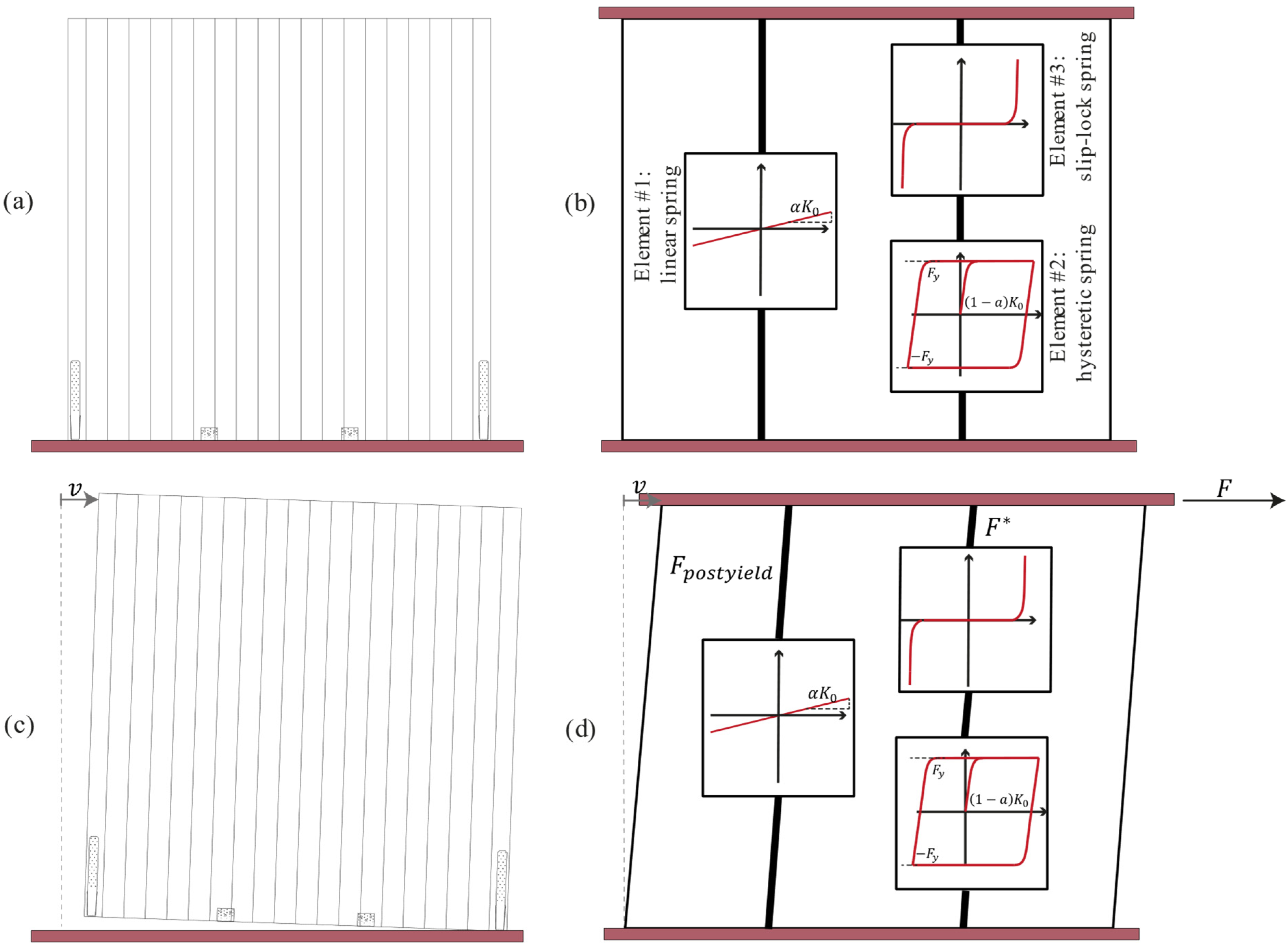
2. A Smooth Hysteretic Model (SHM) for Modeling CLT Walls
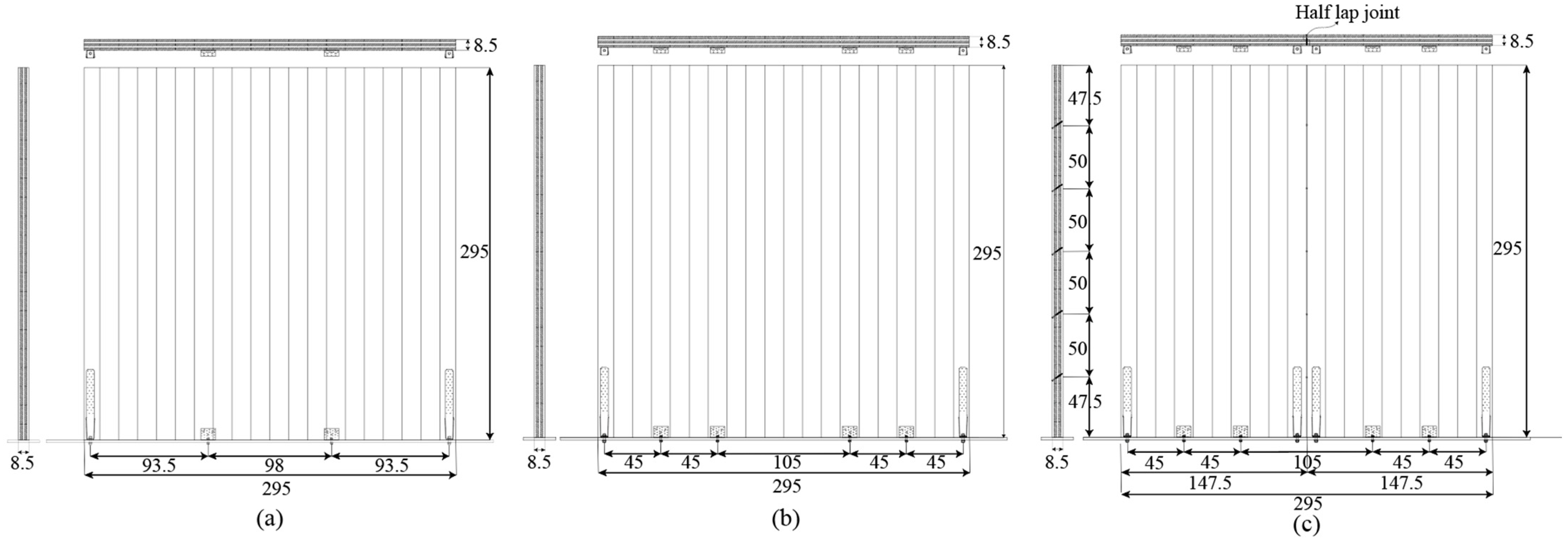
2.1. Brief Description of CLT Shear Walls
2.2. A Numerical Formulation to Represent the Lateral Response of CLT Walls
2.3. State-Space Approach to Solve Equations Governing the SHM
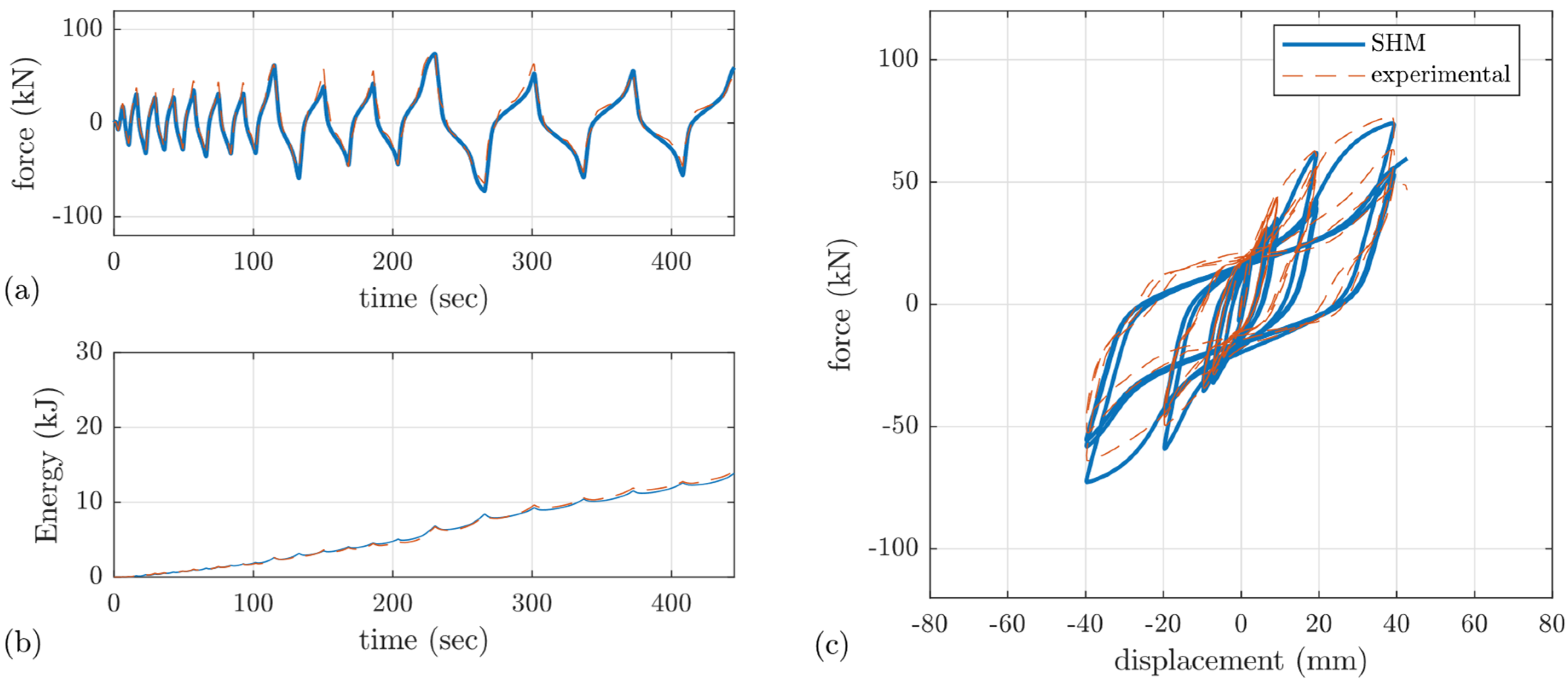
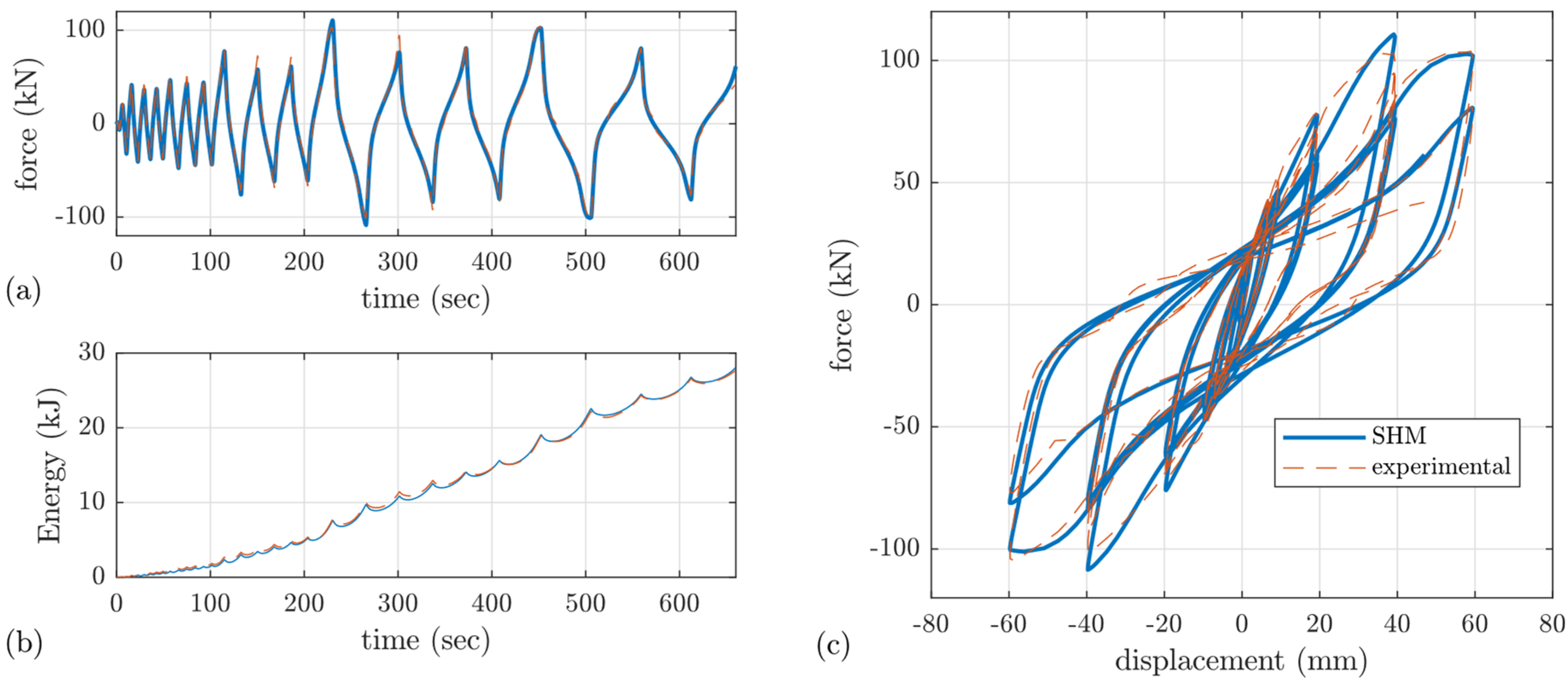
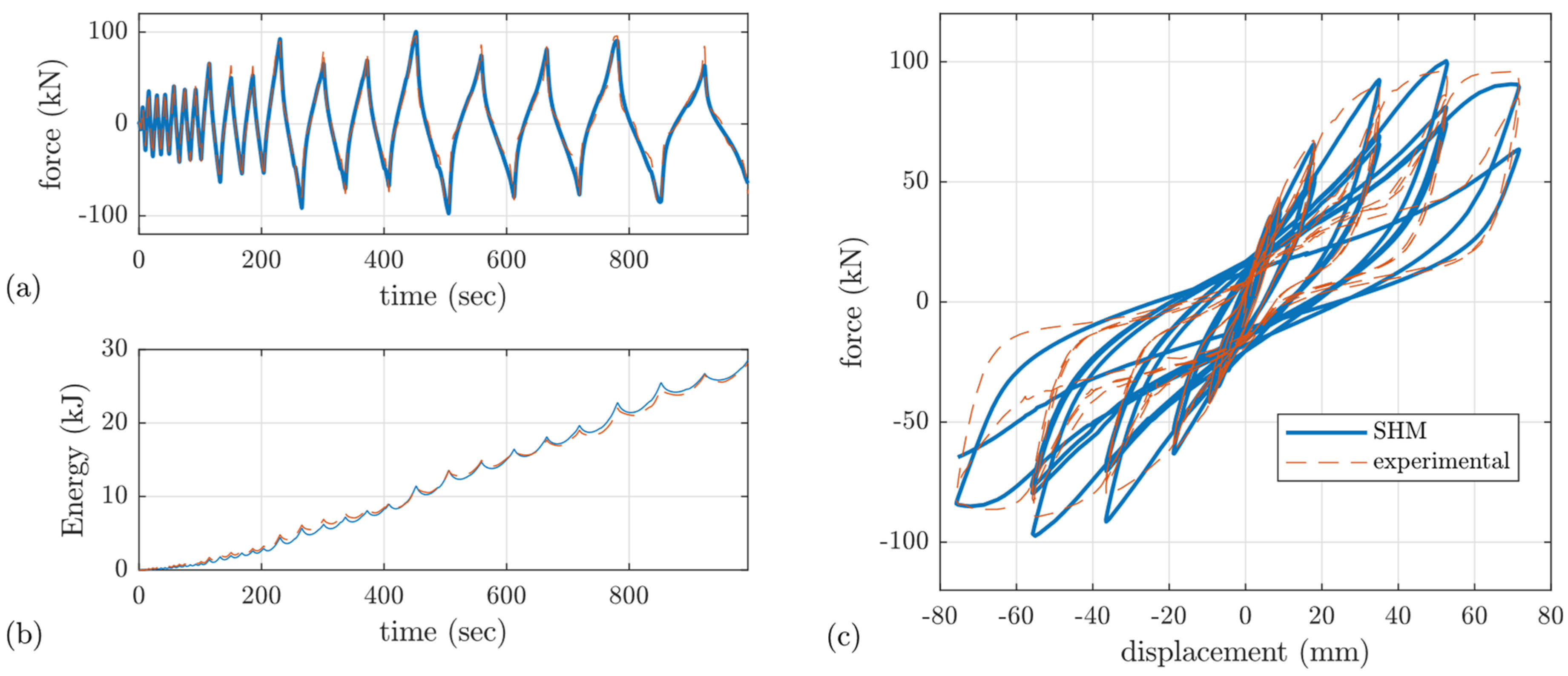
2.4. Model Validation
3. Equivalent Model of a Timber Structure Equipped with Frictional Bearings
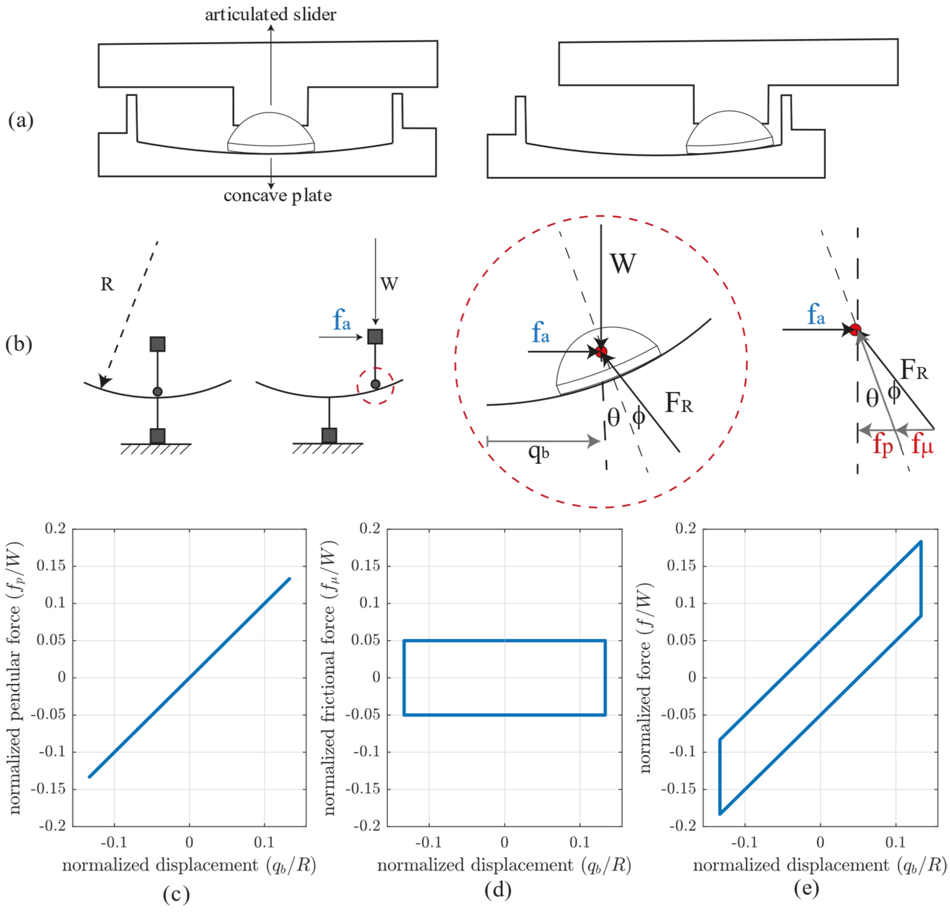
3.1. Brief Description of the Friction Pendulum System (FPS)
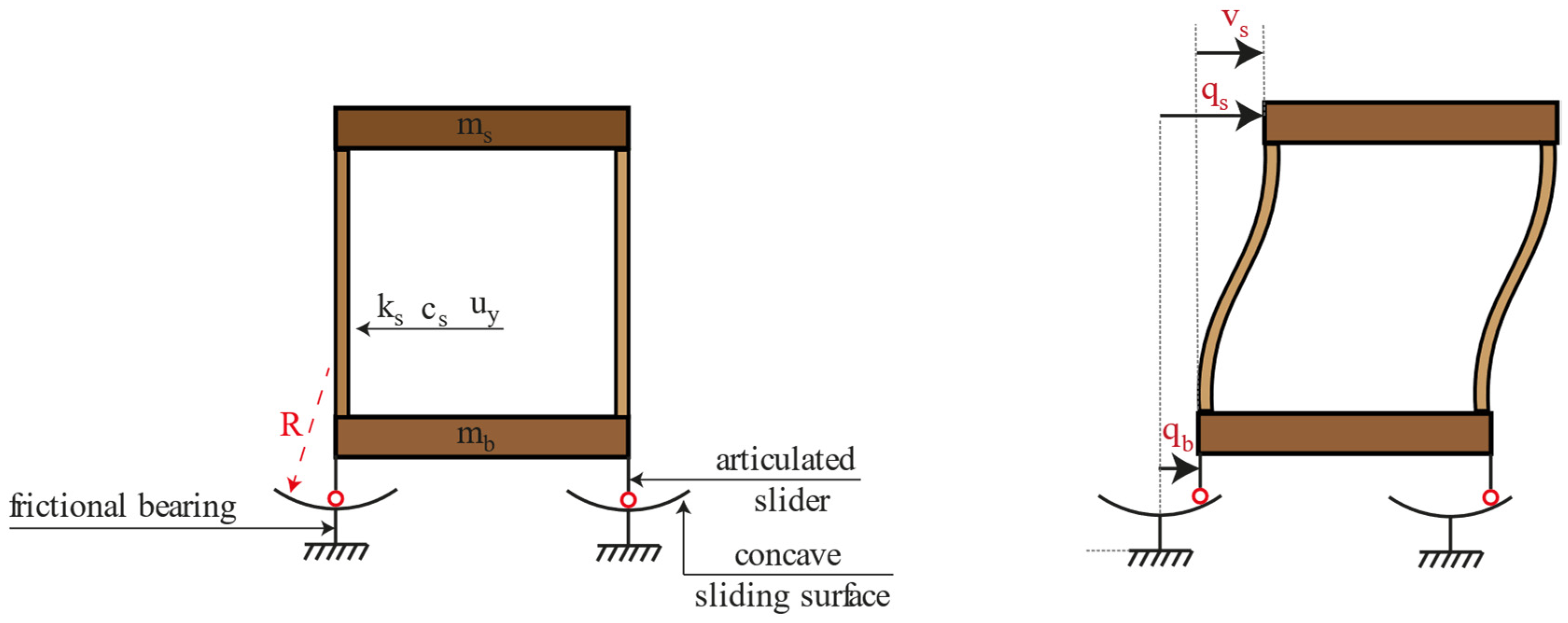
3.2. Equivalent Model of CLT Structure Equipped with FPS Bearings
3.3. Equation of Motion of the Equivalent Model and a Solving Strategy
3.4. Time–History Examples
4. Uncertainties Within the Seismic Fragility Assessment
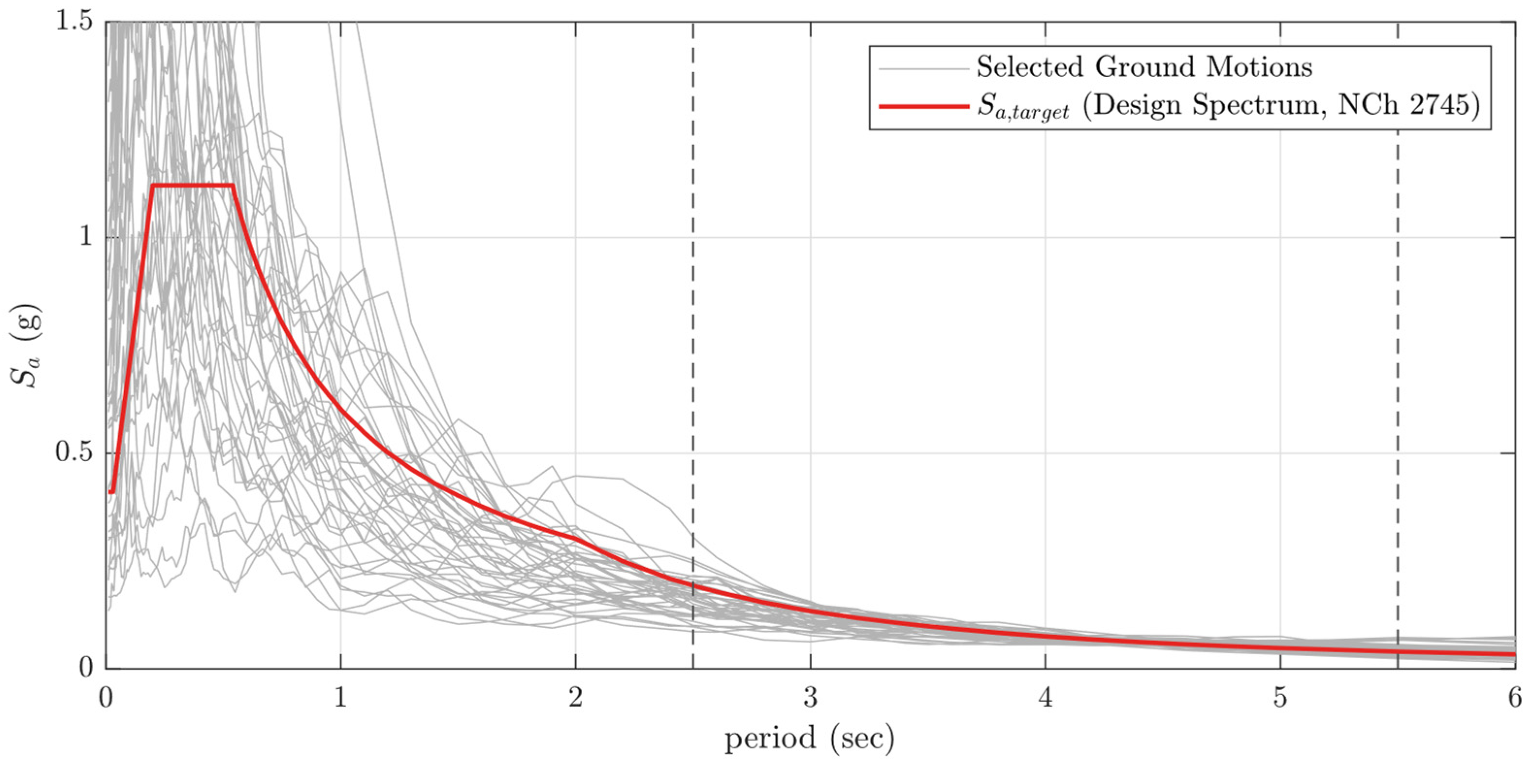
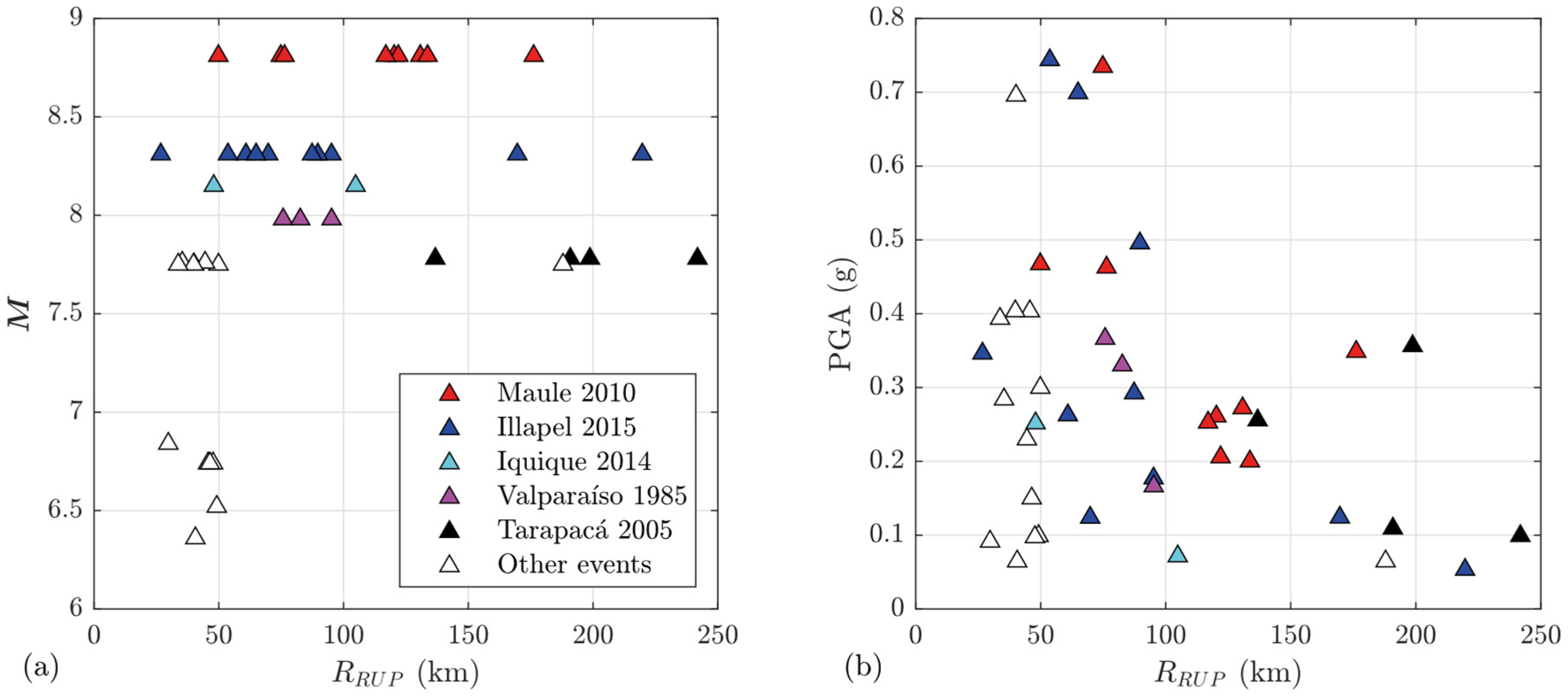
5. Ground Motion Selection
6. Parametric Study
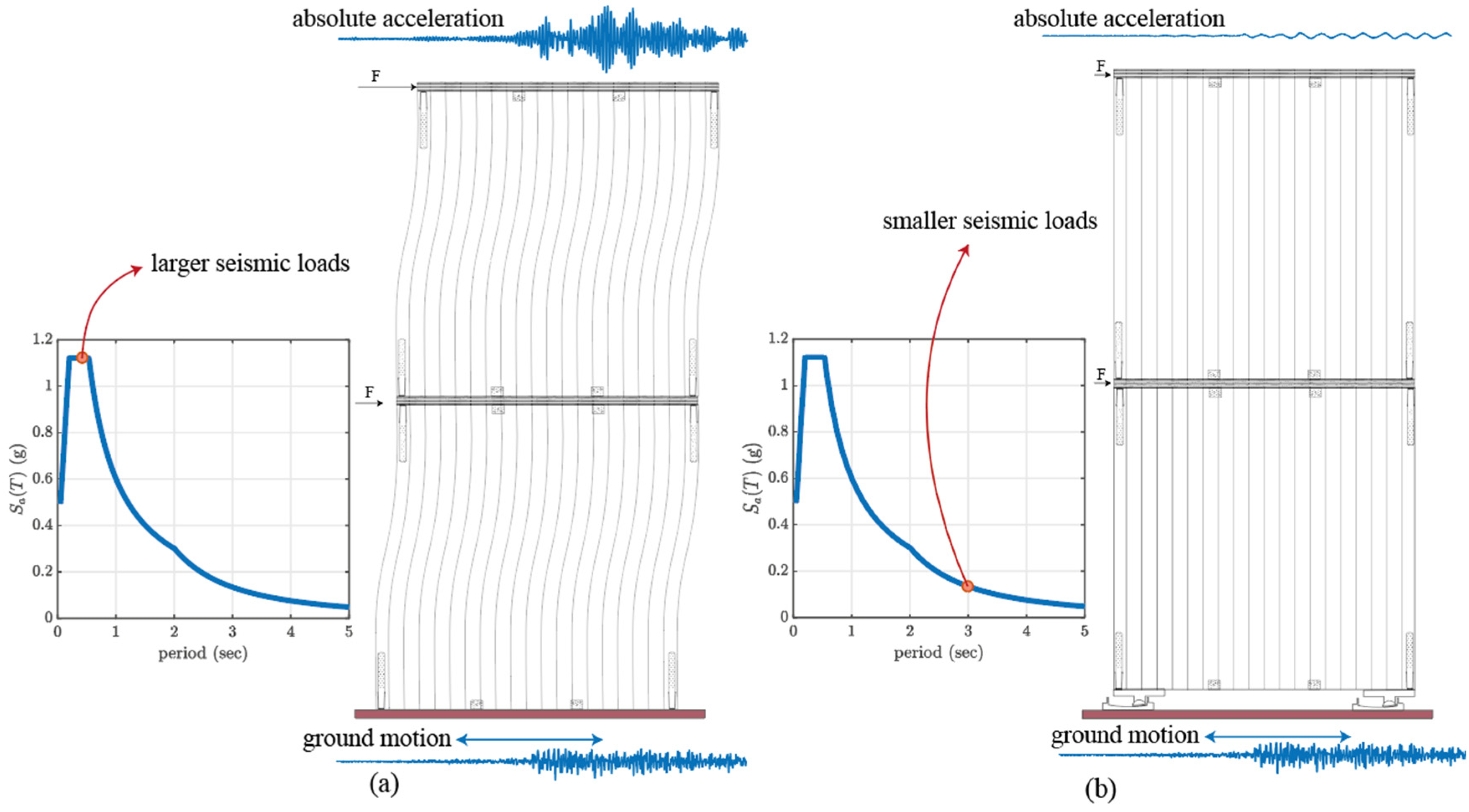
7. Design of Base-Isolated Buildings
8. Seismic Fragility of CLT Structures Equipped with Pendulum Frictional Bearings
8.1. Incremental Dynamic Analyses (IDAs)
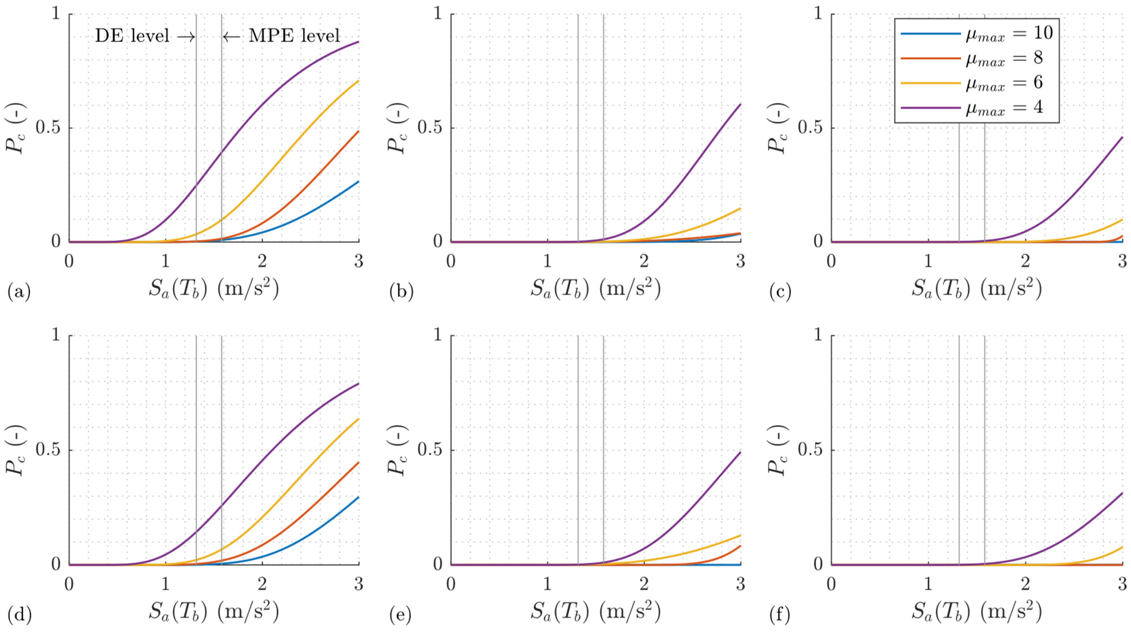
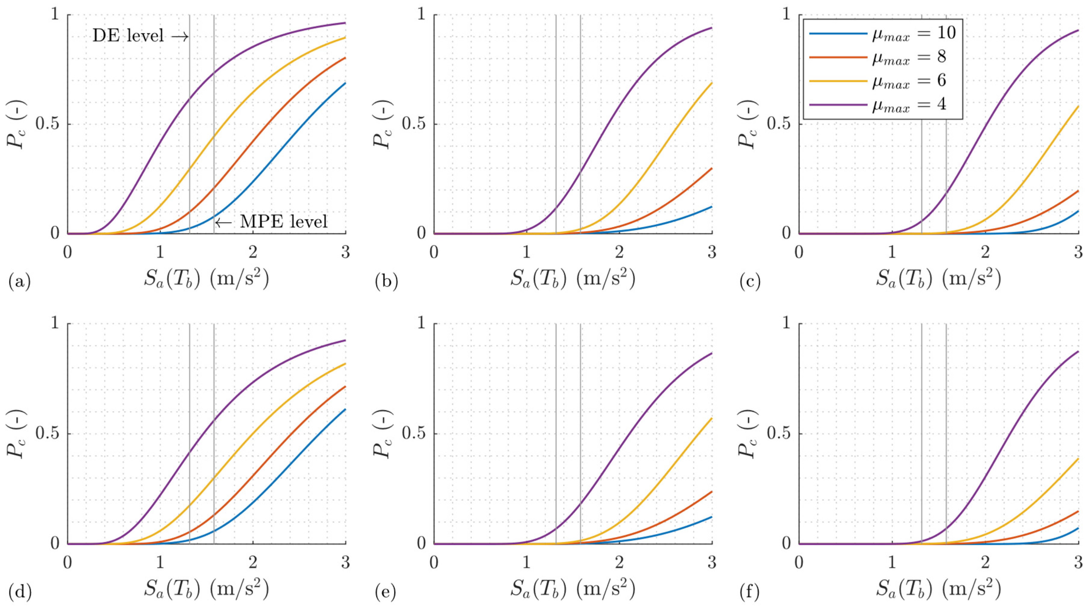
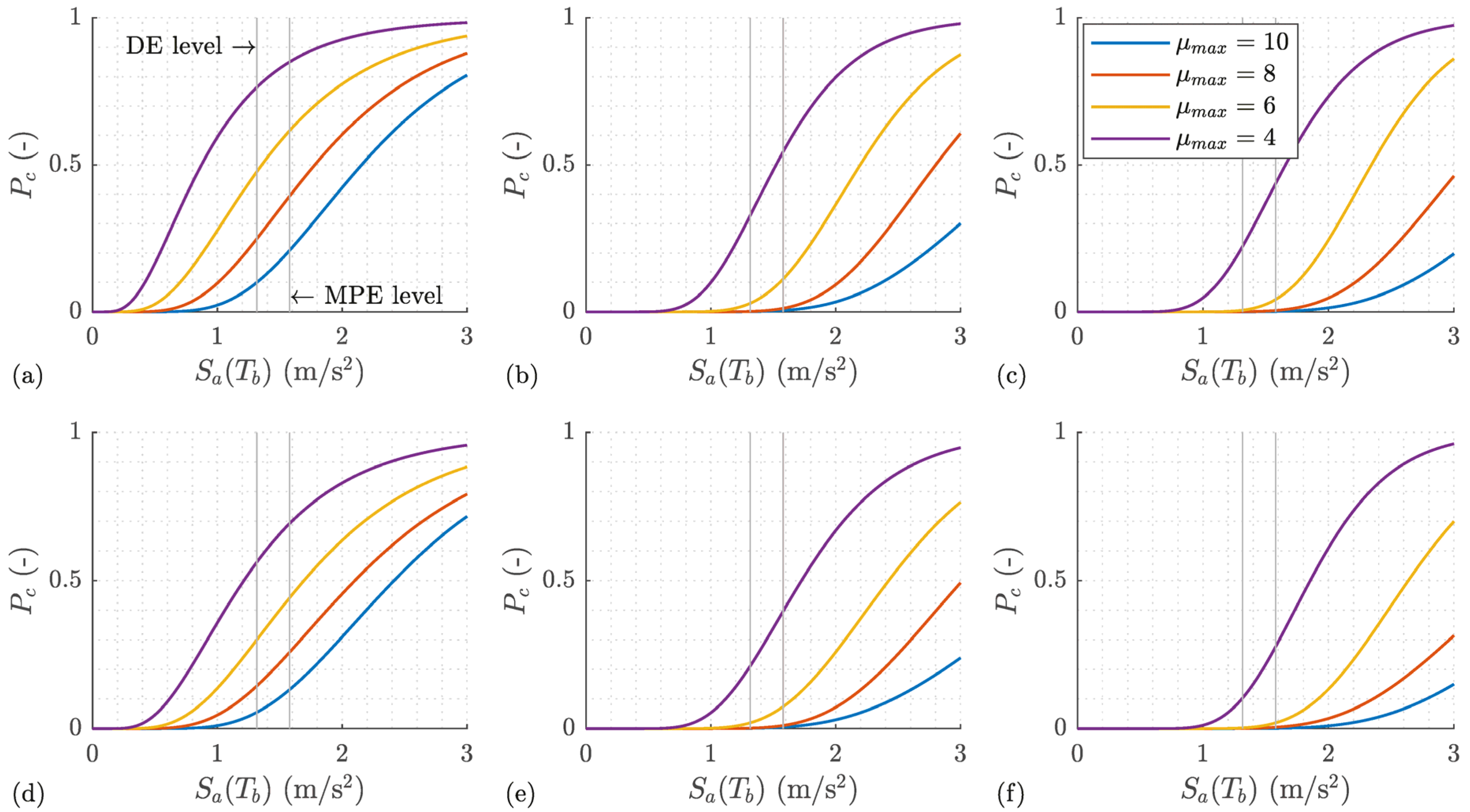
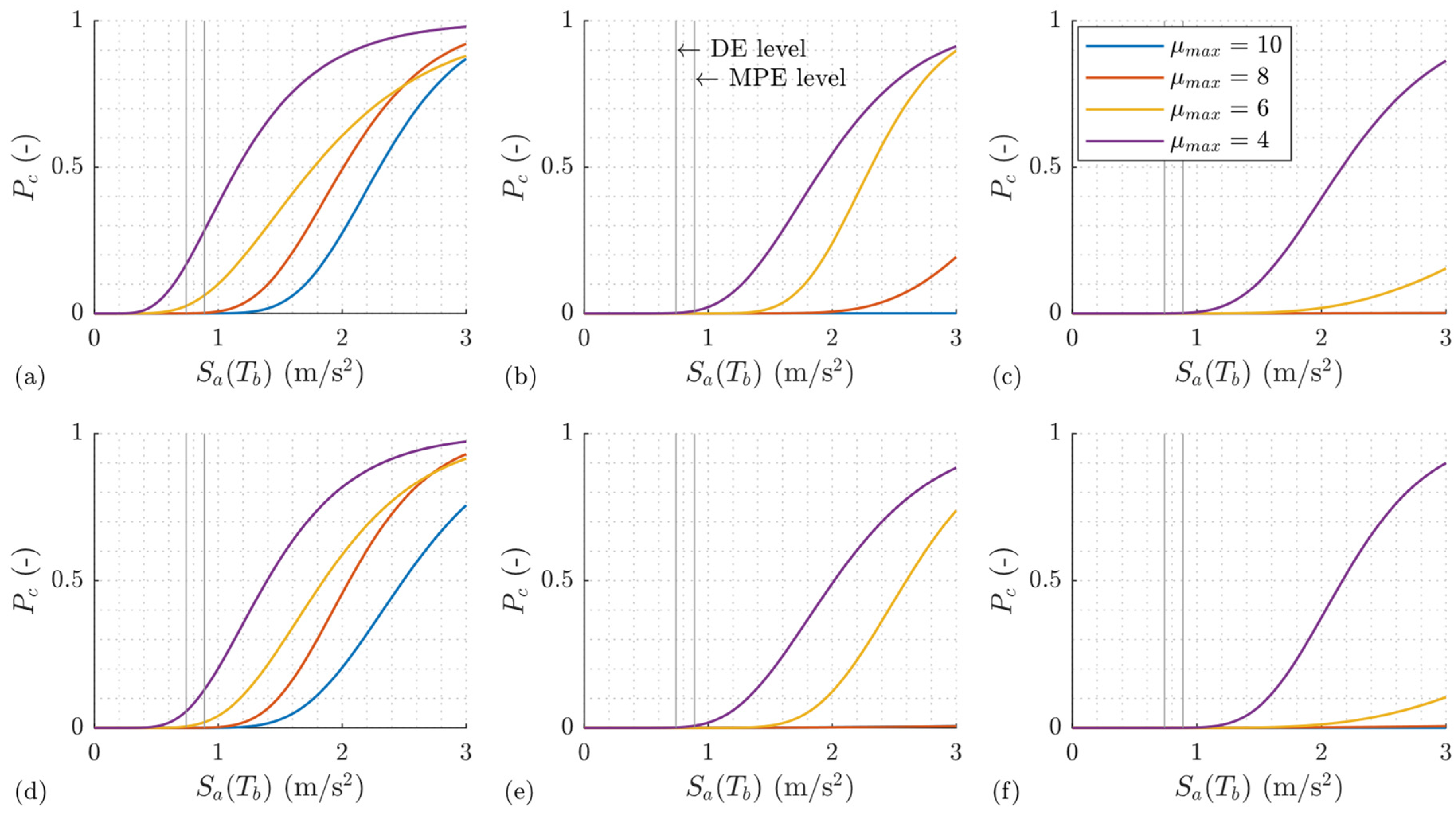
8.2. Fragility Analyses Results and Discussion
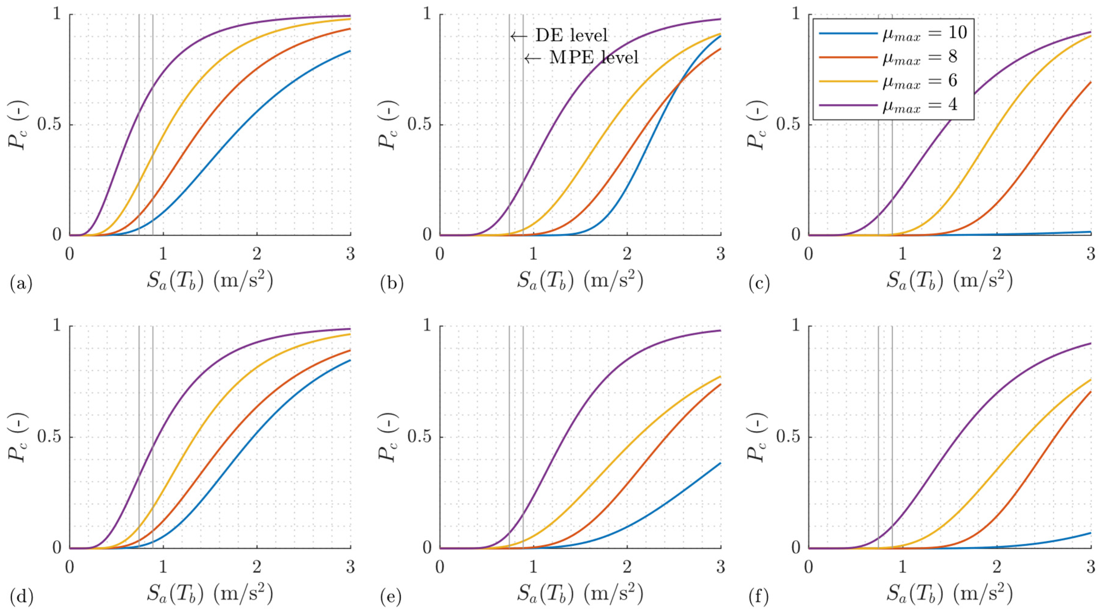
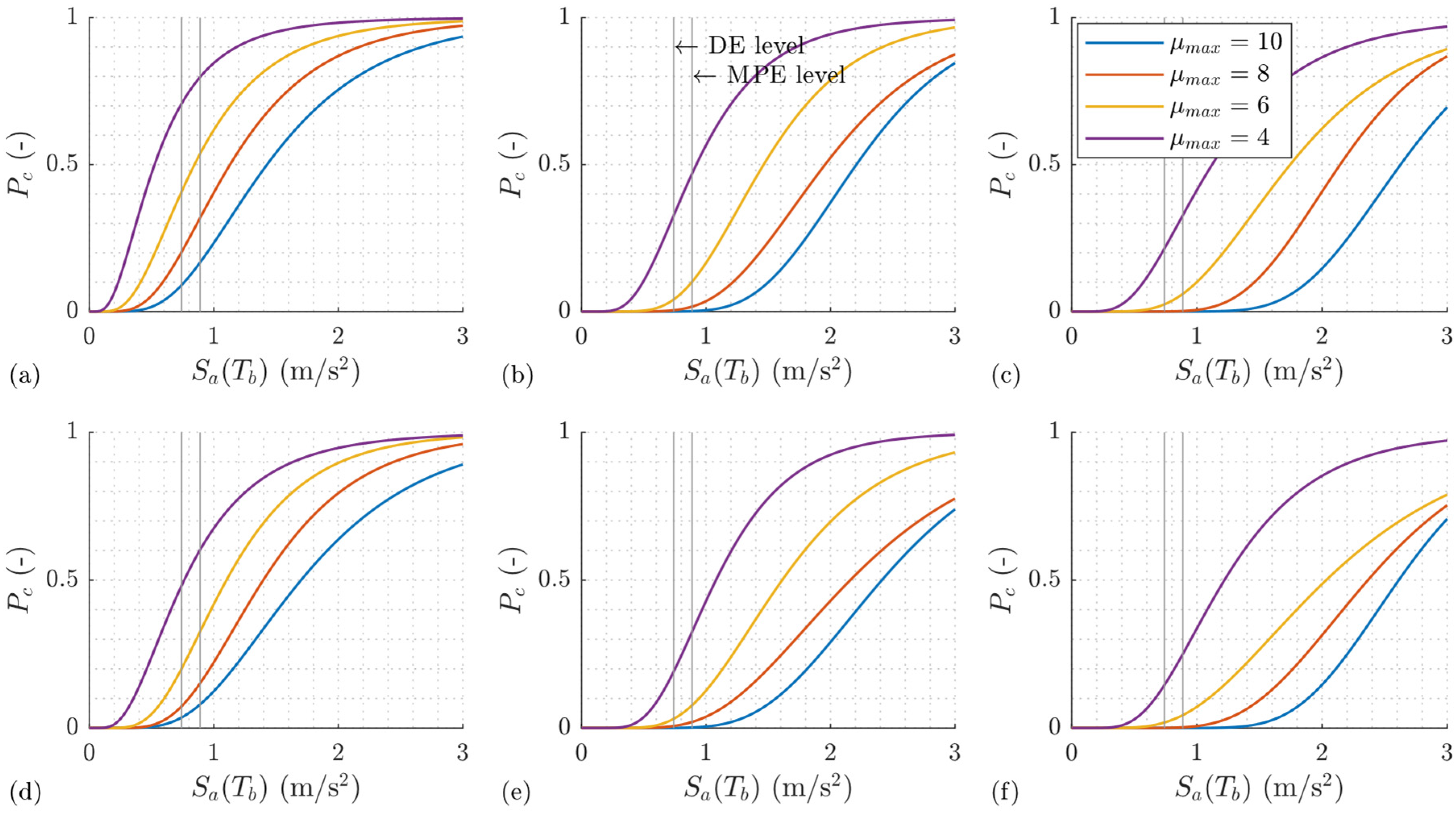
- Better seismic performance is achieved for more flexible superstructures ( s) due to a larger yield displacement required during the design process, a slightly better seismic performance is achieved for larger mass distribution ratios) and larger isolated period ( s).
- If the superstructure is designed to behave elastically at the Design Earthquake level (), an excellent seismic performance is observed in non-stiff structures ( s) or if the superstructure has a middle to high maximum ductility capacity ().
- For rigid CLT superstructures ( s), designs with and a ductility capacity of are required to achieve acceptable seismic performance.
- For flexible CLT superstructures ( s), designs with and a ductility capacity of are necessary to achieve acceptable seismic performance.
- For larger values of the reduction factor , the role of the maximum ductility capacity is crucial, especially for a stiff superstructure (s).
- A reduction factor of , the maximum value allowable according to the Chilean code of base-isolated buildings, is not recommended for stiff structures ( s) or for superstructures with low maximum ductility capacity ().
9. Conclusions
Author Contributions
Funding
Data Availability Statement
Conflicts of Interest
Nomenclature
| Post-yield stiffness ratio of the SHM | |
| Parameter linked to the isolation system’s hysteresis | |
| Superstructure’s damping coefficient | |
| Damping matrix | |
| Design base displacement | |
| Energy’s Normalized Root Mean Square error | |
| Force’s Normalized Root Mean Square error | |
| Lateral force acting on the isolation system | |
| Friction coefficient at large velocity | |
| Friction coefficient at slow velocity | |
| Pendular force of the FPS | |
| Force developed on the superstructure | |
| Friction force of the FPS | |
| Total force of the SHM | |
| Linear post-yield force of the SHM | |
| Reaction force of the FPS | |
| Total yield force of the SHM | |
| Hysteretic force of the SHM | |
| Yield force of the hysteretic spring | |
| Current positive force | |
| Current negative force | |
| Initial positive yield force | |
| Initial negative yield force | |
| Gravity acceleration | |
| Hysteretic cumulative energy dissipated | |
| Cumulative energy causing the failure | |
| Isolation degree | |
| Superstructure’s stiffness | |
| Tangent stiffness of the SHM | |
| Stiffness of the FPS | |
| Stiffness of the hysteretic spring | |
| Stiffness of the linear spring | |
| Stiffness of the slip-lock spring | |
| Initial stiffness of the SHM | |
| Kinematic transformation matrix of the isolation system | |
| Kinematic transformation matrix of the superstructure | |
| Base mass | |
| Roof mass | |
| Total mass of the superstructure | |
| Sample lognormal mean | |
| Mass matrix | |
| Mass of the FPS | |
| Parameter controlling the elastic–plastic transition branches | |
| Probability exceeding a limit state | |
| Base displacement | |
| Roof displacement | |
| Radius of curvature of the FPS | |
| Input influence vector | |
| Reduction factor | |
| Pivot stiffness degradation parameter | |
| Parameter representing pinching | |
| Slip length | |
| Spectral acceleration | |
| Record’s spectral acceleration | |
| Target spectral acceleration | |
| Scale factor | |
| Time | |
| Time at step | |
| Isolated period | |
| Superstructure’s period | |
| Ground acceleration | |
| Vector containing the displacements of the base-isolated model | |
| Vector containing the acceleration of the base-isolated model | |
| Vector containing the velocities of the base-isolated model | |
| Heaviside function | |
| Displacement of the SHM | |
| Maximum displacement demand | |
| Positive maximum displacement | |
| Negative maximum displacement | |
| Superstructure displacement | |
| Maximum superstructure displacement | |
| Positive ultimate displacement | |
| Negative ultimate displacement | |
| Yield displacement | |
| Time-averaged shear wave velocity in the upper 30 m of depth | |
| Total self-weight | |
| Hysteretic parameter of the isolation system | |
| State vector of the base-isolated | |
| State vector of the SHM | |
| Stiffness degradation parameter | |
| Parameter linked to the isolation system’s hysteresis | |
| Ductility-based strength degradation parameter | |
| Energy-based strength degradation parameter | |
| Mass ratio | |
| Average spectral deviation index | |
| Displacement that triggers the sliding phase | |
| ( | Multi-linear objective function |
| Parameter representing pinching | |
| Maximum ductility demand | |
| Friction coefficient of the FPS | |
| Maximum ductility capacity | |
| Superstructure’s critical damping ratio | |
| Parameter representing pinching | |
| Lognormal standard deviation of the sample | |
| , | Hysteric parameter of the unloading curve |
Appendix A

| Definition of the parameters of the SHM |
| are given (Equation (2)) (Equation (3)) (Equation (5)) (Equation (6)) (Equation (7)) (Equation (9)) (Equation (12)) (Equation (13)) (Equation (14)) (Equation (14)) (Equation (15)) |
| Repetition for next step and repeat steps 3.1 to 3.12. |
Appendix B
| NGA-Sub RSN | Date (yyyy-mm-dd) | UTC (hh:mm) | Moment Magnitude | (km) | Station Name | (m/s) | PGA (g) | SF | |
|---|---|---|---|---|---|---|---|---|---|
| 6001795 | 1985-03-03 | 22:47 | 7.98 | 83 | SAN FERNANDO EDIFICIO MUNICIPAL | 688 | 0.33 | 0.63 | 2.45 |
| 6001753 | 1985-03-03 | 22:47 | 7.98 | 95 | TALCA COLEGIO INTEGRADO SAN PIO X | 662 | 0.17 | 0.83 | 5.63 |
| 6001752 | 1985-03-03 | 22:47 | 7.98 | 76 | SAN FELIPE ESCUELA No 6 | 622 | 0.37 | 0.68 | 3.04 |
| 6001151 | 2005-06-13 | 22:44 | 7.78 | 137 | IQUIQUE PLAZA | 605 | 0.26 | 0.78 | 4.41 |
| 6001148 | 2005-06-13 | 22:44 | 7.78 | 191 | EL LOA ADUANA (SMA-1) | 586 | 0.11 | 0.82 | 5.38 |
| 6001155 | 2005-06-13 | 22:44 | 7.78 | 199 | POCONCHILE RETEN DE CARABINEROS | 560 | 0.36 | 0.64 | 2.74 |
| 6001141 | 2005-06-13 | 22:44 | 7.78 | 242 | TAC1 | 568 | 0.10 | 0.77 | 4.20 |
| 6001228 | 2007-11-14 | 15:40 | 7.75 | 34 | MEJILLONES HOSPITAL | 745 | 0.39 | 0.35 | 1.04 |
| 6001234 | 2007-11-14 | 15:40 | 7.75 | 40 | TOCOPILLA | 605 | 0.70 | 0.66 | 2.90 |
| 6001224 | 2007-11-14 | 15:40 | 7.75 | 50 | EL LOA ADUANA (SMA-1) | 586 | 0.30 | 0.82 | 5.09 |
| 6001233 | 2007-11-14 | 15:40 | 7.75 | 188 | SAN PEDRO DE ATACAMA | 745 | 0.06 | 0.64 | 2.57 |
| 6001235 | 2007-11-14 | 15:40 | 7.75 | 40 | TOCOPILLA PUERTO (SOQUIMICH) | 605 | 0.40 | 0.78 | 4.47 |
| 6001240 | 2007-11-15 | 15:03 | 6.36 | 41 | MEJILLONES HOSPITAL | 745 | 0.06 | 0.76 | 3.63 |
| 6001241 | 2007-11-15 | 15:05 | 6.84 | 30 | MEJILLONES HOSPITAL | 745 | 0.09 | 0.64 | 2.47 |
| 6001244 | 2007-12-16 | 08:09 | 6.74 | 46 | MEJILLONES PUERTO | 745 | 0.40 | 0.30 | 1.38 |
| 6001243 | 2007-12-16 | 08:09 | 6.74 | 46 | MEJILLONES | 745 | 0.15 | 0.33 | 1.32 |
| 6001242 | 2007-12-16 | 08:09 | 6.74 | 48 | MEJILLONES HOSPITAL | 745 | 0.10 | 0.48 | 1.37 |
| 6001819 | 2010-02-27 | 06:34 | 8.81 | 176 | PAPUDO LICEO NUESTRA SRA DEL CARMEN | 821 | 0.35 | 0.71 | 3.28 |
| 6001815 | 2010-02-27 | 06:34 | 8.81 | 76 | CURICO HOSPITAL | 514 | 0.46 | 0.32 | 1.20 |
| 6001804 | 2010-02-27 | 06:34 | 8.81 | 117 | ANTU | 622 | 0.25 | 0.29 | 1.40 |
| 6001800 | 2010-02-27 | 06:34 | 8.81 | 131 | LACH | 574 | 0.27 | 0.35 | 1.51 |
| 6001805 | 2010-02-27 | 06:34 | 8.81 | 134 | CLCH | 619 | 0.20 | 0.36 | 1.52 |
| 6001816 | 2010-02-27 | 06:34 | 8.81 | 50 | HUALANE HOSPITAL | 530 | 0.47 | 0.38 | 1.46 |
| 6001811 | 2010-02-27 | 06:34 | 8.81 | 122 | MET | 598 | 0.21 | 0.38 | 1.54 |
| 6001823 | 2010-02-27 | 06:34 | 8.81 | 120 | HSOT | 524 | 0.26 | 0.40 | 1.63 |
| 6001807 | 2010-02-27 | 06:34 | 8.81 | 75 | MELP | 598 | 0.73 | 0.47 | 1.77 |
| 6005167 | 2013-10-31 | 23:03 | 6.52 | 49 | C13O | 505 | 0.10 | 0.84 | 6.36 |
| 6001373 | 2014-04-01 | 23:46 | 8.15 | 48 | HMBCX | 743 | 0.25 | 0.60 | 2.48 |
| 6001395 | 2014-04-01 | 23:46 | 8.15 | 105 | TAC1 | 568 | 0.07 | 0.81 | 5.34 |
| 6002206 | 2014-04-03 | 02:43 | 7.76 | 44 | HMBCX | 743 | 0.23 | 0.76 | 3.97 |
| 6004761 | 2014-04-03 | 02:43 | 7.76 | 35 | T03A | 613 | 0.28 | 0.80 | 4.83 |
| 6002262 | 2015-09-16 | 22:54 | 8.31 | 87 | GO04 | 605 | 0.29 | 0.48 | 1.92 |
| 6002241 | 2015-09-16 | 22:54 | 8.31 | 65 | CO03 | 704 | 0.70 | 0.56 | 2.20 |
| 6005371 | 2015-09-16 | 22:54 | 8.31 | 27 | CO06 | 605 | 0.35 | 0.60 | 2.44 |
| 6005360 | 2015-09-16 | 22:54 | 8.31 | 54 | C11O | 626 | 0.74 | 0.63 | 2.51 |
| 6005364 | 2015-09-16 | 22:54 | 8.31 | 61 | C20O | 737 | 0.26 | 0.76 | 4.03 |
| 6002253 | 2015-09-16 | 22:54 | 8.31 | 170 | MT05 | 571 | 0.12 | 0.79 | 4.63 |
| 6005362 | 2015-09-16 | 22:54 | 8.31 | 90 | C18O | 605 | 0.50 | 0.80 | 4.80 |
| 6005369 | 2015-09-16 | 22:54 | 8.31 | 70 | C33O | 587 | 0.12 | 0.80 | 4.94 |
| 6005358 | 2015-09-16 | 22:54 | 8.31 | 95 | C09O | 754 | 0.18 | 0.81 | 4.90 |
| 6002237 | 2015-09-16 | 22:54 | 8.31 | 220 | AC04 | 605 | 0.05 | 0.83 | 5.56 |
References
- Pei, S.; van De Lindt, J.W.; Popovski, M. Approximate R-Factor for Cross-Laminated Timber Walls in Multistory Buildings. J. Archit. Eng. 2013, 19, 245–255. [Google Scholar] [CrossRef]
- Hammond, G.P.; Jones, C.I. Embodied energy and carbon in construction materials. Proc. Inst. Civil. Eng. Energy 2008, 161, 87–98. [Google Scholar] [CrossRef]
- Arroyo, D.; Ordaz, M.; Teran-Gilmore, A. Seismic loss estimation and environmental issues. Earthq. Spectra 2015, 31, 1285–1308. [Google Scholar] [CrossRef]
- Gavric, I.; Fragiacomo, M.; Ceccotti, A. Cyclic behavior of typical screwed connections for cross-laminated (CLT) structures. Eur. J. Wood Wood Prod. 2015, 73, 179–191. [Google Scholar] [CrossRef]
- Gavric, I.; Fragiacomo, M.; Ceccotti, A. Cyclic behaviour of typical metal connectors for cross-laminated (CLT) structures. Mater. Struct./Mater. Constr. 2015, 48, 1841–1857. [Google Scholar] [CrossRef]
- Gavric, I.; Fragiacomo, M.; Ceccotti, A. Cyclic Behavior of CLT Wall Systems: Experimental Tests and Analytical Prediction Models. J. Struct. Eng. 2015, 141, 04015034. [Google Scholar] [CrossRef]
- Shahnewaz, M.; Dickof, C.; Tannert, T. Experimental investigation of the hysteretic behaviour of single-story single- and coupled-panel CLT shear walls with nailed connections. Eng. Struct. 2023, 291, 116443. [Google Scholar] [CrossRef]
- Wright, T.; Li, M.; Moroder, D.; Lim, H.; Carradine, D. Cyclic behaviour of CLT shear wall hold-down connections using mixed angle self-tapping screws. Eng. Struct. 2023, 286, 116123. [Google Scholar] [CrossRef]
- Dong, H.; He, M.; Wang, X.; Christopoulos, C.; Li, Z.; Shu, Z. Development of a uniaxial hysteretic model for dowel-type timber joints in OpenSees. Constr. Build. Mater. 2021, 288, 123112. [Google Scholar] [CrossRef]
- Folz, B.; Filiatrault, A. Cyclic Analysis of Wood Shear Walls. J. Struct. Eng. 2001, 127, 433. [Google Scholar] [CrossRef]
- Folz, B.; Filiatrault, A. Seismic Analysis of Woodframe Structures. I: Model Formulation. J. Struct. Eng. 2004, 130, 1353–1360. [Google Scholar] [CrossRef]
- Chacón, M.F.; Guindos, P. ASPID: An asymmetric pinching damaged hysteresis model for timber structures. Constr. Build. Mater. 2023, 404, 133106. [Google Scholar] [CrossRef]
- Malo, K.A.; Abrahamsen, R.B.; Bjertnæs, M.A. Some structural design issues of the 14-storey timber framed building “Treet” in Norway. Eur. J. Wood Wood Prod. 2016, 74, 407–424. [Google Scholar] [CrossRef]
- Li, H.; Wang, B.J.; Wei, P.; Wang, L. Cross-laminated Timber (CLT) in China: A State-of-the-Art. J. Bioresour. Bioprod. 2019, 4, 22–30. [Google Scholar] [CrossRef]
- Fast, P.; Gafner, B.; Jackson, R.; Li, J. Case Study: An 18 Storey Tall Mass Timber Hybrid Student Residence at the University of British Columbia, Vancouver. In Proceedings of the World Conference on Timber Engineering, Vienna, Austria, 22–25 August 2016. [Google Scholar]
- Evison, D.C.; Kremer, P.D.; Guiver, J. Mass timber construction in Australia and New Zealand-status, and economic and environmental influences on adoption. Wood Fiber Sci. 2018, 50, 128–138. [Google Scholar] [CrossRef]
- Passarelli, R.N.; Koshihara, M. The Implementation of Japanese CLT: Current Situation and Future Tasks. In Proceedings of the 2018 World Conference on Timber Engineering, Seoul, Republic of Korea, 20–23 August 2018. [Google Scholar]
- Bita, H.M.; Tannert, T. Disproportionate collapse prevention analysis for a mid-rise flat-plate cross-laminated timber building. Eng. Struct. 2019, 178, 460–471. [Google Scholar] [CrossRef]
- Sato, M.; Isoda, H.; Araki, Y.; Nakagawa, T.; Kawai, N.; Miyake, T. A seismic behavior and numerical model of narrow paneled cross-laminated timber building. Eng. Struct. 2019, 179, 9–22. [Google Scholar] [CrossRef]
- Aloisio, A.; Pasca, D.; Tomasi, R.; Fragiacomo, M. Dynamic identification and model updating of an eight-storey CLT building. Eng. Struct. 2020, 213, 110593. [Google Scholar] [CrossRef]
- Polastri, A.; Izzi, M.; Pozza, L.; Loss, C.; Smith, I. Seismic analysis of multi-storey timber buildings braced with a CLT core and perimeter shear-walls. Bull. Earthq. Eng. 2019, 17, 1009–1028. [Google Scholar] [CrossRef]
- Demirci, C.; Málaga-Chuquitaype, C.; Macorini, L. Seismic drift demands in multi-storey cross-laminated timber buildings. Earthq. Eng. Struct. Dyn. 2018, 47, 1014–1031. [Google Scholar] [CrossRef]
- Demirci, C.; Málaga-Chuquitaype, C.; Macorini, L. Seismic shear and acceleration demands in multi-storey cross-laminated timber buildings. Eng. Struct. 2019, 198, 109467. [Google Scholar] [CrossRef]
- Ceccotti, A.; Sandhaas, C.; Okabe, M.; Yasumura, M.; Minowa, C.; Kawai, N. SOFIE project—3D shaking table test on a seven-storey full-scale cross-laminated timber building. Earthq. Eng. Struct. Dyn. 2013, 42, 2003–2021. [Google Scholar] [CrossRef]
- Siembieda, W.; Johnson, L.; Franco, G. Rebuild fast but rebuild better: Chile’s initial recovery following the 27 February 2010 earthquake and tsunami. Earthq. Spectra 2012, 28, 621–641. [Google Scholar] [CrossRef]
- Ugalde, D.; Luis Almazán, J.; Santa María, H.; Guindos, P. Seismic protection technologies for timber structures: A review. Eur. J. Wood Wood Prod. 2019, 77, 173–194. [Google Scholar] [CrossRef]
- Bolvardi, V.; Pei, S.; van de Lindt, J.W.; Dolan, J.D. Direct displacement design of tall cross laminated timber platform buildings with inter-story isolation. Eng. Struct. 2018, 167, 740–749. [Google Scholar] [CrossRef]
- Chen, Z.; Popovski, M.; Ni, C. A novel floor-isolated re-centering system for prefabricated modular mass timber construction-Concept development and preliminary evaluation. Eng. Struct. 2020, 222, 111168. [Google Scholar] [CrossRef]
- Medel-Vera, C.; Carolina Contreras, M. Resilience-based predictive models for the seismic behaviour of mid-rise, base-isolated CLT buildings for social housing applications in Chile. J. Build. Eng. 2021, 44, 2352–7102. [Google Scholar] [CrossRef]
- Auad, G.; Almazán, J.L.; Tapia, N.; Quizanga, D. Static and dynamic experimental validations of a frictional isolator with improved internal lateral impact behavior. Soil Dyn. Earthq. Eng. 2024, 181, 108637. [Google Scholar] [CrossRef]
- Quizanga, D.; Almazán, J.L.; Valdivieso, D.; López-García, D.; Guindos, P. Shaking table test of a timber building equipped with a novel cost-effective, impact-resilient seismic isolation system. J. Build. Eng. 2024, 82, 108402. [Google Scholar] [CrossRef]
- Lukacs, I.; Björnfot, A.; Tomasi, R. Strength and stiffness of cross-laminated timber (CLT) shear walls: State-of-the-art of analytical approaches. Eng. Struct. 2019, 178, 136–147. [Google Scholar] [CrossRef]
- Sivaselvan, M.; Reinhorn, A. Hysteretic Models for Deteriorating Inelastic Structures. J. Eng. Mech. 2000, 126, 633. [Google Scholar] [CrossRef]
- Simeonov, V.K.; Sivaselvan, M.V.; Reinhorn, A.M. Nonlinear analysis of structural frame systems by the state-space approach. Comput.-Aided Civ. Infrastruct. Eng. 2000, 15, 76–89. [Google Scholar] [CrossRef]
- Hunt, B.R.; Lipsman, R.L.; Rosenberg, J.M.; Coombes, K.R.; Osborn, J.E.; Stuck, G.J. A Guide to MATLAB®; Cambridge University Press: Cambridge, UK, 2006. [Google Scholar] [CrossRef]
- Zayas, V.A.; Low, S.S.; Mahin, S.A. A Simple Pendulum Technique for Achieving Seismic Isolation. Earthq. Spectra 1990, 6, 317–333. [Google Scholar] [CrossRef]
- Auad, G.; Castaldo, P.; Almazán, J.L. Seismic reliability of structures equipped with LIR-DCFP bearings in terms of superstructure ductility and isolator displacement. Earthq. Eng. Struct. Dyn. 2022, 51, 3171–3214. [Google Scholar] [CrossRef]
- Castaldo, P.; Alfano, G. Seismic reliability-based design of hardening and softening structures isolated by double concave sliding devices. Soil Dyn. Earthq. Eng. 2020, 129, 105930. [Google Scholar] [CrossRef]
- Castaldo, P.; Tubaldi, E. Influence of FPS bearing properties on the seismic performance of base-isolated structures. Earthq. Eng. Struct. Dyn. 2015, 44, 2817–2836. [Google Scholar] [CrossRef]
- Castaldo, P.; Ripani, M. Optimal design of friction pendulum system properties for isolated structures considering different soil conditions. Soil Dyn. Earthq. Eng. 2016, 90, 74–87. [Google Scholar] [CrossRef]
- Castaldo, P.; Tubaldi, E. Influence of ground motion characteristics on the optimal single concave sliding bearing properties for base-isolated structures. Soil Dyn. Earthq. Eng. 2018, 104, 346–364. [Google Scholar] [CrossRef]
- Castaldo, P.; Amendola, G.; Palazzo, B. Seismic fragility and reliability of structures isolated by friction pendulum devices: Seismic reliability-based design (SRBD). Earthq. Eng. Struct. Dyn. 2017, 46, 425–446. [Google Scholar] [CrossRef]
- Almazán, J.L.; De la Llera, J.C. Physical model for dynamic analysis of structures with FPS isolators. Earthq. Eng. Struct. Dyn. 2003, 32, 1157–1184. [Google Scholar] [CrossRef]
- Weisman, J.; Warn, G.P. Stability of Elastomeric and Lead-Rubber Seismic Isolation Bearings. J. Struct. Eng. 2012, 138, 215–223. [Google Scholar] [CrossRef]
- Kalfas, K.N.; Ghorbani Amirabad, N.; Forcellini, D. The role of shear modulus on the mechanical behavior of elastomeric bearings when subjected to combined axial and shear loads. Eng. Struct. 2021, 248, 113248. [Google Scholar] [CrossRef]
- Constantinou, M.; Mokha, A.; Reinhorn, A. Teflon Bearings in Base Isolation II: Modeling. J. Struct. Eng. 1990, 116, 455–474. [Google Scholar] [CrossRef]
- Park, Y.J.; Wen, Y.K.; Ang, A.H.-S. Random vibration of hysteretic systems under bi-directional ground motions. Earthq. Eng. Struct. Dyn. 1986, 14, 543–557. [Google Scholar] [CrossRef]
- Luco, J.E. Effects of soil-structure interaction on seismic base isolation. Soil Dyn. Earthq. Eng. 2014, 66, 167–177. [Google Scholar] [CrossRef]
- Auad, G.A.; Castaldo, P.; Almazán, J.L. Seismic reliability of reinforced moment frame equipped with Lateral Impact Resilient frictional isolators. In Proceedings of the 14th fib PhD Symposium in Civil Engineering, Rome, Italy, 5–7 September 2022. [Google Scholar]
- Auad, G.A.; Castaldo, P.; Almazán, J.L. Seismic reliability of reinforced concrete structures with Lateral Impact Resilient Double Concave Frictional Isolators. In Proceedings of the 2nd fib Italy YMG Symposium on Concrete and Concrete Structures, Rome, Italy, 18–19 November 2021. [Google Scholar]
- Bozorgnia, Y.; Abrahamson, N.A.; Ahdi, S.K.; Ancheta, T.D.; Al Atik, L.; Archuleta, R.J.; Atkinson, G.M.; Boore, D.M.; Campbell, K.W.; Chiou, B.S.-J.; et al. NGA-Subduction research program. Earthq. Spectra 2022, 38, 783–798. [Google Scholar] [CrossRef]
- NCh2745-2003; Análisis y Diseño de Edificios con Aislación Sísmica. Instituto Nacional de Normalización: Santiago, Chile, 2003.
- Palazzo, B. Seismic behavior of base isolated buildings. In Proceedings of the International Meeting on Earthquake Protection of Buildings, Ancona, Italy, 22 April 1991; Available online: https://stacks.stanford.edu/file/fm826wn5553/TR132_Gupta.pdf (accessed on 11 March 2025).
- Gupta, A. Seismic Demands for Performance Evaluation of Steel Moment Resisting Frame Structures; Stanford University: Stanford, CA, USA, 1999. [Google Scholar]
- Mokha, A.; Constantinou, M.; Reinhorn, A. Teflon Bearings in Base Isolation I: Testing. J. Struct. Eng. 1990, 116, 438–454. [Google Scholar] [CrossRef]
- Castaldo, P.; Palazzo, B.; Alfano, G.; Palumbo, M.F. Seismic reliability-based ductility demand for hardening and softening structures isolated by friction pendulum bearings. Struct. Control Health Monit. 2018, 25, 2256. [Google Scholar] [CrossRef]
- Castaldo, P.; Palazzo, B.; Ferrentino, T. Seismic reliability-based ductility demand evaluation for inelastic base-isolated structures with friction pendulum devices. Earthq. Eng. Struct. Dyn. 2017, 46, 1245–1266. [Google Scholar] [CrossRef]
- McKay, M.D.; Beckman, R.J.; Conover, W.J. A comparison of three methods for selecting values of input variables in the analysis of output from a computer code. Technometrics 2000, 42, 55–61. [Google Scholar] [CrossRef]
- Vořechovský, M.; Novák, D. Correlation control in small-sample Monte Carlo type simulations I: A simulated annealing approach. Probabilistic Eng. Mech. 2009, 24, 452–462. [Google Scholar] [CrossRef]
- Iervolino, I.; De Luca, F.; Cosenza, E. Spectral shape-based assessment of SDOF nonlinear response to real, adjusted and artificial accelerograms. Eng. Struct. 2010, 32, 2776–2792. [Google Scholar] [CrossRef]
- Molazadeh, M.; Saffari, H. The effects of ground motion duration and pinching-degrading behavior on seismic response of SDOF systems. Soil Dyn. Earthq. Eng. 2018, 114, 333–347. [Google Scholar] [CrossRef]
- Demir, A.; Palanci, M.; Kayhan, A.H. Evaluation of Supplementary Constraints on Dispersion of EDPs Using Real Ground Motion Record Sets. Arab. J. Sci. Eng. 2020, 45, 8379–8401. [Google Scholar] [CrossRef]
- Boore, D.M. Orientation-independent, nongeometric-mean measures of seismic intensity from two horizontal components of motion. Bull. Seismol. Soc. Am. 2010, 100, 1830–1835. [Google Scholar] [CrossRef]
- Vamvatsikos, D.; Cornell, C.A. Incremental dynamic analysis. Earthq. Eng. Struct. Dyn. 2002, 31, 491–514. [Google Scholar] [CrossRef]
- Castaldo, P.; Ripani, M.; Priore, R.L. Influence of soil conditions on the optimal sliding friction coefficient for isolated bridges. Soil Dyn. Earthq. Eng. 2018, 111, 131–148. [Google Scholar] [CrossRef]
- Karavasilis, T.L.; Seo, C.Y. Seismic structural and non-structural performance evaluation of highly damped self-centering and conventional systems. Eng. Struct. 2011, 33, 2248–2258. [Google Scholar] [CrossRef]

| Test ID | Number of Hold-Downs | Number of Angle Brackets | Number of Screws in Vertical Joints | Vertical Load (kN/m) | Predominant Deformation | Panel Interaction |
|---|---|---|---|---|---|---|
| Test-01 | 2 | 2 | - | 18.5 | Sliding | Single |
| Test-02 | 2 | 4 | - | 18.5 | Rocking–sliding | Single |
| Test-03 | 4 | 4 | 5 | 18.5 | Rocking | Couple |
| Test ID | (kN/mm) | (kN) | (mm) | (kJ) | (mm) | ||||||||
|---|---|---|---|---|---|---|---|---|---|---|---|---|---|
| Test-01 | 5 | 0.35 | 0.13 | 0.22 | 0.30 | 0.30 | 10.50 | 153.3 | 96 | 43.3 | 8 | 12 | 5 |
| Test-02 | 5 | 0.37 | 0.21 | 0.20 | 0.30 | 0.30 | 10.52 | 136.7 | 91 | 62.2 | 13 | 7 | 5 |
| Test-03 | 8 | 0.38 | 0.25 | 0.15 | 0.26 | 0.24 | 9.00 | 131.4 | 94.9 | 63.3 | 14.6 | 7 | 5 |
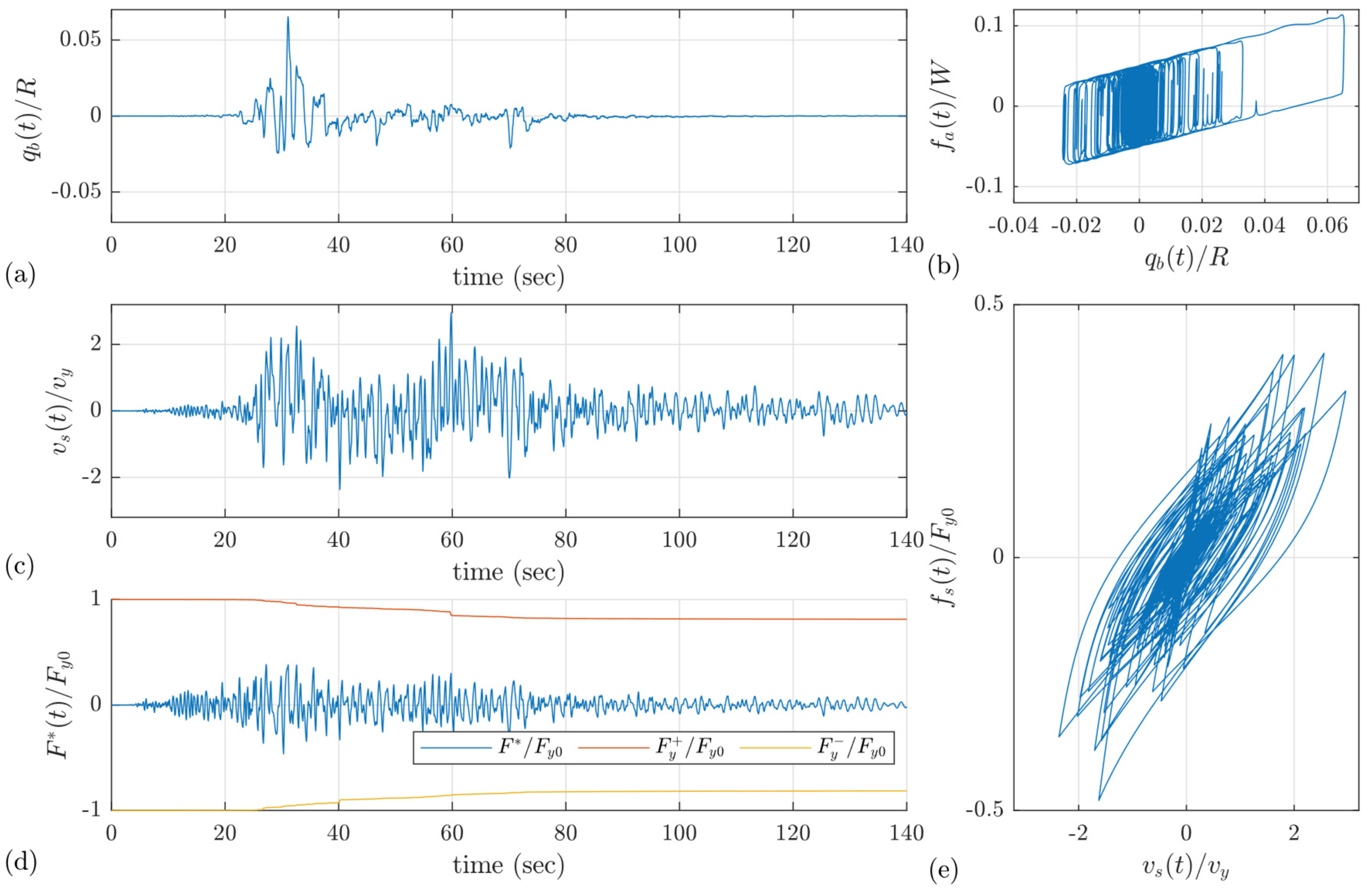
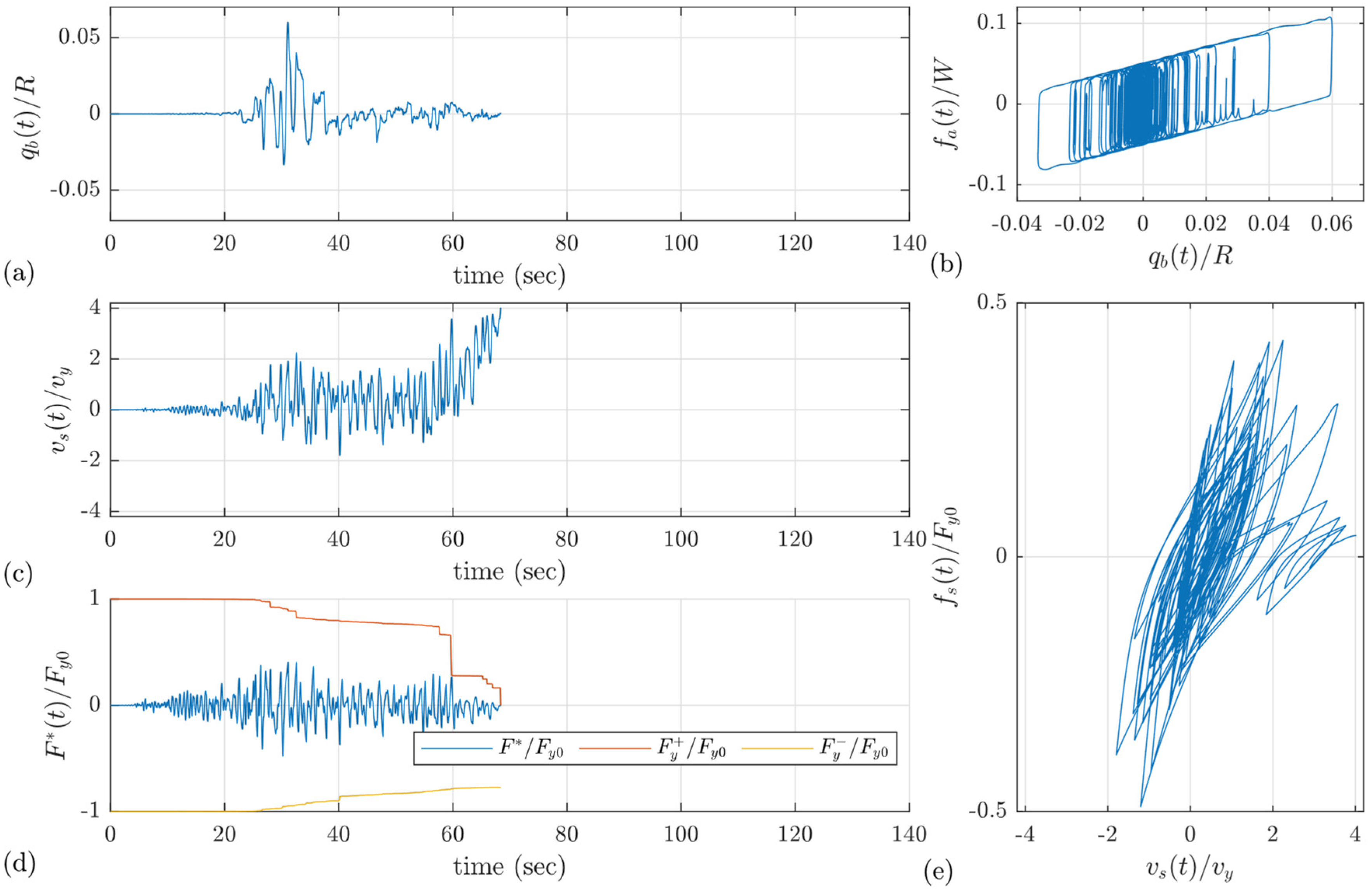
| Time–History Example Shown in | Maximum | Collapse | Positive Strength Degradation | Negative Strength Degradation | |
|---|---|---|---|---|---|
| Figure 10 | 6.0 | No | 2.9 | 0.81 | 0.82 |
| Figure 11 | 4.0 | Yes | 4.0 | 0.00 | 0.77 |
| Static Analysis | Time–History Analysis | |||||
|---|---|---|---|---|---|---|
| * | ** | |||||
| (sec) | (cm) | (cm) | (cm) | (cm) | (cm) | |
| 0.7 | 0.3 | 20.6 | 0.6 | 20.5 | 0.4 | 0.8 |
| 0.6 | 20.6 | 2.4 | 20.1 | 1.8 | 3.1 | |
| 0.9 | 20.6 | 5.4 | 19.7 | 3.8 | 5.9 | |
| 0.9 | 0.3 | 20.6 | 0.6 | 20.4 | 0.4 | 0.6 |
| 0.6 | 20.6 | 2.4 | 20.0 | 1.6 | 2.2 | |
| 0.9 | 20.6 | 5.4 | 19.4 | 3.5 | 4.7 | |
| Static Analysis | Time–History Analysis | |||||
|---|---|---|---|---|---|---|
| * | ** | |||||
| (sec) | (cm) | (cm) | (cm) | (cm) | (cm) | |
| 0.7 | 0.3 | 14.6 | 0.4 | 18.0 | 0.3 | 0.8 |
| 0.6 | 14.6 | 1.7 | 17.8 | 1.3 | 3.0 | |
| 0.9 | 14.6 | 3.9 | 17.6 | 2.7 | 5.9 | |
| 0.9 | 0.3 | 14.6 | 0.4 | 18.0 | 0.3 | 0.5 |
| 0.6 | 14.6 | 1.7 | 17.9 | 1.0 | 2.1 | |
| 0.9 | 14.6 | 3.9 | 17.3 | 2.3 | 4.4 | |
Disclaimer/Publisher’s Note: The statements, opinions and data contained in all publications are solely those of the individual author(s) and contributor(s) and not of MDPI and/or the editor(s). MDPI and/or the editor(s) disclaim responsibility for any injury to people or property resulting from any ideas, methods, instructions or products referred to in the content. |
© 2025 by the authors. Licensee MDPI, Basel, Switzerland. This article is an open access article distributed under the terms and conditions of the Creative Commons Attribution (CC BY) license (https://creativecommons.org/licenses/by/4.0/).
Share and Cite
Auad, G.; Valdés, B.; Contreras, V.; Colombo, J.; Almazán, J. Effects of the Ductility Capacity on the Seismic Performance of Cross-Laminated Timber Structures Equipped with Frictional Isolators. Buildings 2025, 15, 1208. https://doi.org/10.3390/buildings15081208
Auad G, Valdés B, Contreras V, Colombo J, Almazán J. Effects of the Ductility Capacity on the Seismic Performance of Cross-Laminated Timber Structures Equipped with Frictional Isolators. Buildings. 2025; 15(8):1208. https://doi.org/10.3390/buildings15081208
Chicago/Turabian StyleAuad, Gaspar, Bastián Valdés, Víctor Contreras, José Colombo, and José Almazán. 2025. "Effects of the Ductility Capacity on the Seismic Performance of Cross-Laminated Timber Structures Equipped with Frictional Isolators" Buildings 15, no. 8: 1208. https://doi.org/10.3390/buildings15081208
APA StyleAuad, G., Valdés, B., Contreras, V., Colombo, J., & Almazán, J. (2025). Effects of the Ductility Capacity on the Seismic Performance of Cross-Laminated Timber Structures Equipped with Frictional Isolators. Buildings, 15(8), 1208. https://doi.org/10.3390/buildings15081208