Abstract
Building vibration induced by running trains or other loads is related to soil vibration, building coupling loss, and the building floor’s amplification factor. In order to predict the vibration response of the proposed building caused by various loads, the propagation law of Rayleigh wave in saturated foundation soil and the refraction and transmission coefficients of Rayleigh wave between saturated soil and building structure are analyzed by using the theoretical analysis method, and the building coupling loss coefficient is obtained. The dynamic equation of the building’s structural vibration is established, and the analytical expression of the floor amplification factor is derived. A frame structure building is selected as the specific research object. Based on the Kirchhoff thin plate theory, the three-dimensional frame structure characteristic matrix of the building is obtained, and the vertical displacement values of each floor of the building under the action of the Ricker pulse load are calculated. The results are compared with the results in the literature, which verifies the effectiveness and accuracy of the transfer function method proposed in this study and fills the gap of insufficient research on the analysis of displacement transfer loss in soil structure interaction (SSI) in the literature.
1. Introduction
Transportation-induced vibrations significantly impact buildings and residents, becoming a key social concern [1]. The dynamic response of buildings to transportation-induced vibrations is a critical research focus due to its impact on structural safety and comfort [2,3]. Accurately predicting the impact of transportation-induced vibrations on buildings remains a major challenge in engineering practice.
Currently, two primary methods are used to predict environmental vibrations caused by trains. The first involves conducting extensive field experiments, collecting large amounts of measured data, and analyzing general patterns. The second is to establish numerical models of soil and buildings to perform simulation analyses and summarize rules from the results.
In field experimentation, vibration data are collected through on-site monitoring and analyzed statistically. For example, Xia He et al. [4] and Cao Yanmei et al. [5] conducted field measurements to analyze the vibration characteristics of railways and high-rise buildings, summarizing the effects of factors such as train speed, axle load, and the distance between tracks and buildings. While reliable, such methods are constrained by testing conditions, costly, and time-consuming. Many researchers have conducted empirical studies on train-induced building vibrations. Masoud et al. [6] measured vibrations from ground and subway trains in six buildings and nearby open spaces, quantifying the differences in vibration levels between the two settings. Galvin [7], Connolly [8], and Zhai [9] examined the effects of high-speed train-induced ground vibrations, exploring relationships with variables such as track design, soil type, and embankment distance. Madshus et al. [10] introduced a building amplification factor to assess peak vibration magnitudes in Norwegian wooden structures situated on soft soil. More recently, in 2021, Sadeghi and team [11,12,13] developed and validated a vibration–acoustic building model, establishing correlations between train-induced vibration acceleration and structural responses, grounded in field test data. Experimental methods, while yielding reliable outcomes, are time-consuming and expensive. Additionally, they are susceptible to external factors like environmental conditions, sensor instability, and background noise, which can contaminate test data and undermine the reliability of the derived prediction equations.
Numerical methods play a crucial role in studying the vibration transmission mechanisms of adjacent buildings. Yao Jinbao [14] developed a spatial dynamic model incorporating the interaction between soil and building foundations, analyzing how different contact conditions and factors influence train-induced building vibrations. Fang Lei [15] simulated SSI by deriving the stiffness coefficient between soil and buildings, further enhancing the prediction model’s accuracy using the random forest algorithm. Auersch [16] examined building vibrations in soils of varying compositions and introduced a streamlined method to account for SSI in layered grounds. Furthermore, Auersch [17] also contributed by developing simplified models to predict building responses to ground vibrations based on empirical transfer functions. Many studies adopt simplified assumptions, failing to account for soil saturation and its dependence on vibration frequency, which can result in inaccuracies under complex conditions. For example, Auersch’s [17] empirical transfer function model did not fully address dispersion effects, leading to potential inaccuracies in predicting vibration responses across different frequency ranges.
To establish a more comprehensive understanding of how vibrations propagate from external sources to buildings, it is crucial to consider not only the direct transmission of vibrations through soil and structures but also the radiation of energy into the surrounding environment. An important aspect that has been widely studied is the way energy radiates into the ground from vibrating bodies such as trains and buildings, and how this radiation affects nearby structures. By understanding these radiation effects, researchers can refine predictive models and develop more accurate methods for evaluating and mitigating vibration impacts. The radiation of energy into the ground by vibrating bodies, such as trains and buildings, and their subsequent effects on nearby structures have been widely studied. For example, Vogiatzis [18] employed a three-phase approach: utilizing a finite element model (FEM) to compute vibrations at the tunnel–soil interface and investigating how metro systems generate ground-borne vibrations and propagate them into surrounding environments, emphasizing the role of SSI and the amplification of vibrations within buildings. Similarly, Colaco et al. [19] employed hybrid numerical–experimental models to assess railway-induced vibrations, providing insights into energy transmission pathways and vibration attenuation through soil layers. Improving SSI research on the propagation mechanism of energy radiated to the ground by vibrating bodies (such as trains and buildings) has been explored in the existing research. Araz et al. [20] introduced a method for optimizing double-tuned mass dampers (TMDs) while considering SSI. Kanellopoulos et al. [21] explored both linear and nonlinear dynamic interactions between a reactor and auxiliary structures on a realistic layered soil profile, emphasizing the significance of structure–soil–structure interaction (SSSI) modeling. Using realistic geometric assumptions, they developed high-fidelity 3D FEMs of varying complexity within the realistic modeling and simulation of the Earthquake Soil–Structure Interaction (Real-ESSI) Simulator. Their methodology incorporated a hybrid approach, merging numerical and experimental findings with advanced post-processing techniques. This approach revolves around SSI curves derived from experimentally evaluated free-field input motion under real-world conditions [19,22]. However, their method is computationally intensive and relies on detailed site-specific data, making it less practical for general predictive applications. In contrast, this study introduces a unified analytical framework that combines Rayleigh wave propagation, soil–structure coupling loss, and floor amplification effects to predict displacement transfer losses in saturated soils.
As railway-induced vibrations travel through foundations, floors, and spans of adjacent buildings, they may experience amplification or attenuation. Kuo et al. [23] conducted a study on building coupling loss resulting from railway vibrations, utilizing both numerical simulations and experimental measurements. López-Mendoza et al. [24] introduced a transfer function method to predict building vibrations through 3D numerical modeling, considering factors like SSI, floor amplification, and free-field response. The current study complements these efforts by providing a theoretical framework for understanding and predicting SSI and its impact on building vibrations. Yao et al. [25] analytically derived the coupling loss coefficient for buildings situated on elastic foundation soil, offering predictions for train-induced vibrations in buildings. These studies use simplified coupling loss coefficients that do not fully reflect the complexity of SSIs. Moreover, these studies rely on complex numerical models (such as finite element methods) that are computationally expensive, especially when dealing with three-dimensional models or layered soils. By introducing the coupling loss coefficient and floor amplification coefficient, this paper can more accurately predict the amplification or attenuation phenomenon of vibration in different building floors, without complicated numerical models, and the calculation speed is fast, which has the potential to be applied in large-scale projects.
The study builds upon the theoretical work of Lapwood [26] and Maurice James [27] on the reflection and transmission of Rayleigh waves at specific angles. By expanding on their research, the study provides a more detailed analysis of wave propagation in saturated soil and its implications for SSI. Yao [28] introduced a method to minimize stress and displacement residuals on both sides of the contact surface between soil and structure. The current study adopts and further refines Yao’s method, ensuring more accurate predictions of SSI and building vibrations.
Despite progress in understanding soil–structure interactions, key challenges remain. Many studies adopt simplified assumptions, failing to account for soil saturation and its dependence on vibration frequency, which can result in inaccuracies under complex conditions. Most existing numerical models assume homogeneous soil properties, making them less effective in describing vibrations in stratified or complex geological environments. Finite element and hybrid models incur high computational costs, limiting their applicability in large-scale projects, while experimental methods are constrained by environmental conditions and sensor stability, with data quality susceptible to noise interference.
To address these issues, this paper proposes an analytical transfer function method that integrates Rayleigh wave propagation, coupling loss coefficients, and floor amplification effects into a unified theoretical framework. This method not only addresses the limitations of traditional numerical and experimental approaches in terms of frequency-dependent behavior and computational efficiency but also provides more accurate theoretical support and practical guidance. By comparing the proposed method with numerical and experimental results from the literature, this study validates the method’s accuracy and practicality, offering a new direction for research on SSI dynamics.
2. Transfer Function Methodology
The proposed transfer function method offers significant potential for real-world applications, particularly in the design and assessment of vibration mitigation strategies for buildings near transportation infrastructures. For example, it can be applied to predict vibration levels in residential or commercial buildings located adjacent to railways, metro systems, or highways, where traffic-induced vibrations are a major concern. By providing a computationally efficient framework, the method can serve as a valuable tool for engineers to evaluate the impact of proposed infrastructure projects on surrounding structures and design effective vibration isolation systems.
It should be noted that the linear hypothesis is adopted in this study, that is, the vibration response during SSI is assumed to be linear. This hypothesis is suitable for small- and medium-amplitude environmental vibration (such as traffic vibration) scenarios, while transfer function-based methods are generally effective in linear regimes but face challenges when dealing with highly nonlinear behavior, as discussed in Ditommaso et al. [29]. Therefore, this will be included in nonlinear dynamics applied in high-intensity scenarios in the future.
To precisely forecast the effects of environmental vibrations on people’s lives, certain nations employ predictive models to assess their impact. The international standard ISO 14837-1:2005 proposes an important framework for the propagation system. This framework decomposes load-induced vibrations A(f) in the frequency domain into three independent components: the source term S(f), the propagation term P(f), and the receiver term R(f). These components are assumed to be decoupled, as shown in Equation (1).
The U.S. Federal Transportation Administration (FTA) evaluates potential significant ground vibrations based on vibration transmission rates. This system includes four distinct and uncoupled components: the excitation force, the vibration transmission pathway, the building vibrations, and low-frequency noise from secondary radiation. The force density and vibration transmission rate of the vibration source are determined by analog tests and in-situ hammering tests, respectively. The prediction Equation (2) is shown as follows:
where LV is the root mean square prediction speed level; FDL is the force density level of the line vibration source; LSTM is the line source transmissibility; and Cbuilding is the correction coefficient considering SSI and vibration propagation in building floors.
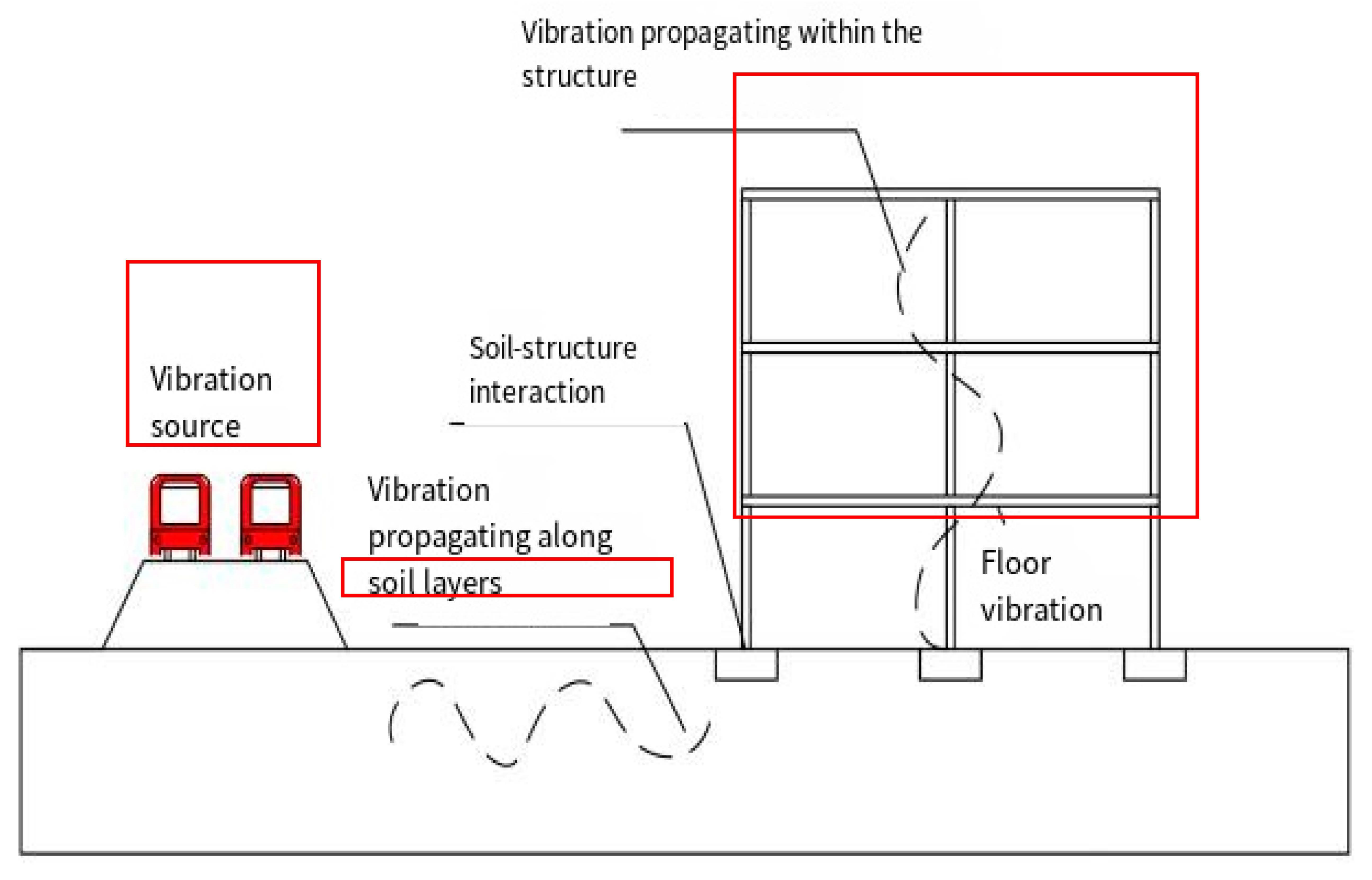
Based on the discussion above, the process of vibration propagation can generally be divided into three main components. The first is the vibration source term, which reflects the frequency characteristics and intensity of the load. The second is the propagation term, which is influenced by soil conditions, topography, and underground structures. Finally, the receiver term depends on the material properties, structural layout, and size of the building. These components collectively determine how vibrations are transmitted and amplified, as illustrated in Figure 1.

Figure 1.
Propagation diagram of vibration induced by high-speed train [25].
This study employs the transfer function approach to establish relationships among the three independent components of the vibration propagation system. Two coefficients are defined: the coupling loss coefficient, Cl, and the floor amplification coefficient, Fa. These coefficients enable the prediction of vibration responses in soil and buildings. The transfer function method is expressed in Equation (3).
where Usoil is free-field vibration, which refers to the vibration of saturated foundation soil caused by arbitrary loads; Cl is the coupling loss coefficient between the soil and structure, reflecting the strength of soil–structure interaction; and Fa is the floor amplification coefficient, reflecting the transmission relationship between the vibration of each floor of the building and the building foundation.
2.1. Derivation of Coupling Loss Coefficient Between Saturated Soil and Buildings
In 1961, Lapwood [26] theoretically examined the reflection and transmission of Rayleigh waves at specific angles, reaching several notable conclusions. Expanding on this research, James [27] further enhanced the understanding of Rayleigh wave reflection and transmission phenomena. Yao [28] introduced a pivotal concept, suggesting that the residual stress and displacement on both sides of the contact surface should ideally be nullified. By selecting suitable transmission and reflection coefficients, Yao’s method minimizes these residuals, allowing for the direct computation of refraction and transmission coefficients without the need for complex waveform conversions. The residual difference of stress and displacement, I0, can be integrated to the minimum value in the sense of least squares according to the following Equation (4):
where I1 and I2 are the integral expressions of stress and displacement generated only by incident. σxx, σxx′, τxz, τxz′, u, u′, w, w′ are the normal stresses, shear stresses, vertical displacements, and horizontal displacements in the two different media, respectively. I1 and I2 can be obtained from Equation (5):
where σxx0, τxz0, u0, and w0 are the normal stresses, shear stresses, vertical displacements, and horizontal displacements at the interface position, respectively.
Rayleigh wave propagation in the saturated half-space is shown in Figure 2.
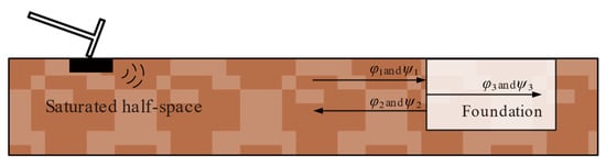
Figure 2.
Schematic diagram of Rayleigh wave propagation on the discontinuous surface of a quarter-space medium.
In Xia [30], potential functions are used to represent displacement and stress. By applying boundary conditions, the potential functions of R waves in saturated soil can be derived. and () can be expressed as:
where ; A1, A2, and A3 are undetermined coefficients independent of coordinate parameter z, and their value can be arbitrarily taken; c is the Rayleigh wave phase velocity (); and .
Introduction of permeability boundary conditions:
Rayleigh equation in saturated half-space can be obtained as:
in which,
where and μ are the Lamb constants of the soil skeleton; n is the porosity, is the density of the water mass; and represent two kinds of P-wave velocity in saturated soil porous media, respectively; is the P-wave velocity of the soil skeleton; is the S-wave velocity in the porous medium of saturated soil; and is the shear transverse wave velocity of the soil skeleton.
It follows that for the right moving wave:
where
Similarly, for the left traveling wave there are:
It follows that for the left traveling wave:
The Rayleigh wave velocity can be numerically solved by selecting the soil layer parameters. Combined with Equation (6) and Equation (9), it can be seen that the wave velocity of the R wave in saturated soil, as well as the wave velocity of the P1 wave, P2 wave, and S wave, are all affected by frequency, which is different from the elastic half-space foundation, that is, the phase velocity of Rayleigh wave in saturated half-space is dispersive.
The wave functions φ3 and ψ3 of Rayleigh waves can be defined as:
where A and B are constants; in kγ = ω/γ, γ represents the Rayleigh wave velocity, and ω is the fluctuation circle.
For elastic media, the characteristic equation of right-traveling Rayleigh waves is as follows:
To obtain:
where , , and are the wave numbers of the R wave, P wave, and S wave under the elastic half-space, respectively, , , and .
According to the theory of Rayleigh wave propagation on discontinuities, it is assumed that when Rayleigh waves and are perpendicular to the soil–building interface at x = 0, a portion of the wave reflects and propagates in the negative x-direction, while another portion scatters and loses energy. The Rayleigh wave reflected through the contact surface and propagating in the negative direction of x is denoted as and , and the transmitted wave propagating forward along the x-axis through the interface is denoted as and . Bring Equations (10) and (13) into Equation (6), and Equation (16) into Equation (14), and the potential function expression of each wave hypothesized above is shown as follows:
where are constants.
For the convenience of calculation, the time factor, is omitted, and the stress and displacement on the left side of x = 0 are shown in the Equations (18)–(21):
The stress and displacement on the right side of x = 0 are shown in Equations (22)–(25):
Stresses and displacements caused by the incident wave (,) are shown by:
By inserting Equations (26)–(29) into Equation (5), one can derive the stress and displacement exclusively induced by the incident Rayleigh wave at the discontinuous surface of the medium.
where ; ; ; ; ; ; ; ; ; ; ; . and represent the parameters of medium two.
Let the reflection coefficient R = A4/A1 and T = A7/A1, and substitute Equations (30) and (31) into Equation (4) to obtain the I0 expression with the unknown parameters R and T. According to the integral property of natural logarithm e, the residual I0 error of stress displacement is simplified, and the final simplified form is as in Equation (32):
where the parameters A~L are all known parameters, which can be obtained from the soil parameters, and the constants can be expressed as:
where l is the in-filled trench depth.
By selecting the appropriate transmission coefficient and reflection coefficient, the displacement stress residual, I0, on both sides of the interface is as close to zero as possible, which can avoid the difficulty of considering the complex waveform conversion and theoretical derivation. By and , the extreme value point of I0 is obtained, and the reflection coefficient R and transmission coefficient T are solved, as shown in Equation (34):
The solution is:
where:
2.2. Derivation of the Building Floor Amplification Factor
The response of the building after receiving an external excitation is not uniform. During the transmission of free-field vibration from foundation to structure, the response of different floors will be significantly different. Specifically, the higher floors tend to experience greater displacement and acceleration than the lower floors, a phenomenon known as the amplification effect. To quantify this effect, the researchers introduced the concept of floor magnification factor to take into account the difference in sensitivity of different floors to vibration in structural design and safety assessment.
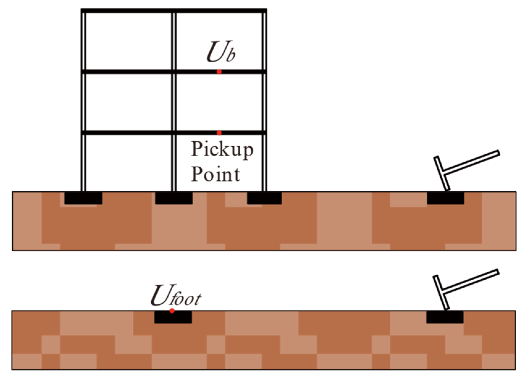
When subjected to vibration source excitation, the ratio of a building floor’s vibration response (displacement, velocity, acceleration, etc.) to the substrate’s response is shown in Figure 3, then the floor amplification factor can be expressed as:
where is the vibration response of a certain floor; and is the vibration response of the substrate. The ratio reflects the relative increase in the response from the ground to the floor.
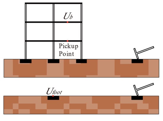
Figure 3.
Schematic diagram of the ground system of the building and the ground system of the building foundation.
The displacement of the building due to the vertical foundation acceleration is governed by the basic equation of structural dynamics, as shown below:
where, [M], [K], and [C] represent the overall stiffness matrix, mass matrix, and damping matrix of the building respectively; ,, and represent the relative displacement, relative velocity, and relative acceleration of each node of the building relative to the foundation vibration; represents the vertical acceleration excitation of the foundation; is a column vector with values of 1 in all rows, of the same order as the stiffness matrix.
The basic equations of structural dynamics in the frequency domain are obtained by doing the Fourier transform of Equation (39):
And because:
where is the absolute displacement of the building.
According to the definition in Equation (37) of the floor amplification factor, the analytical expression of the floor amplification factor can be obtained by combining Equations (39) and (40):
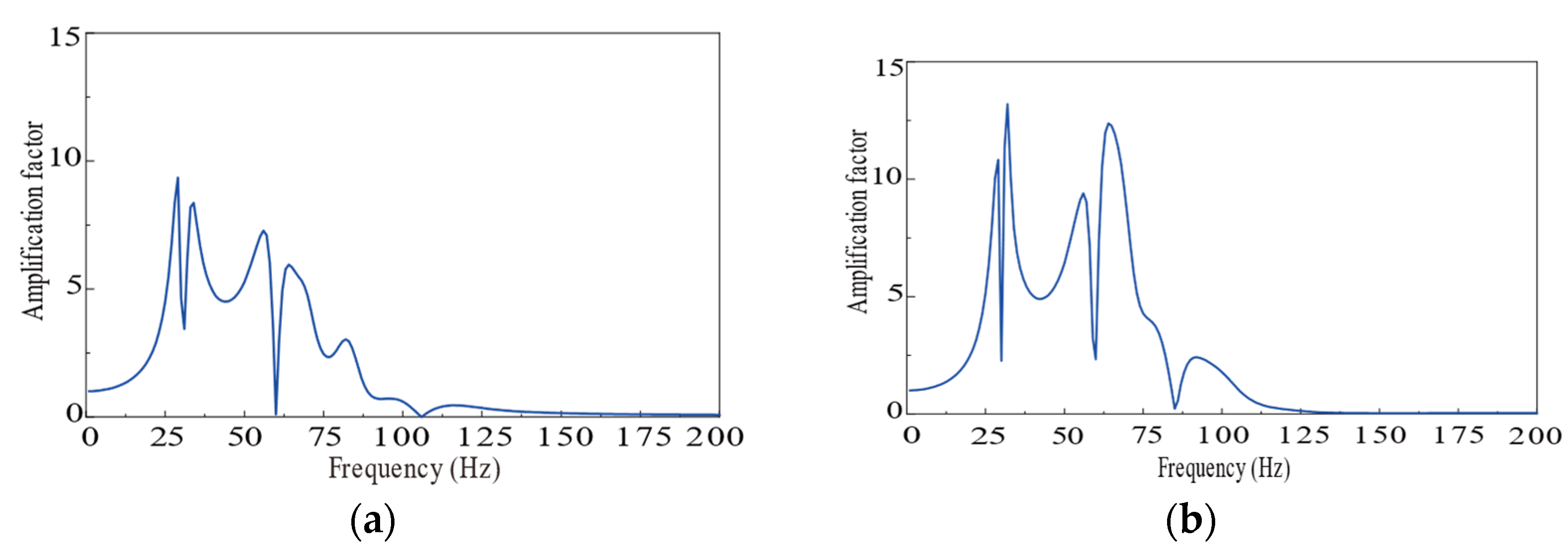
The floor amplification factor, as derived from Equation (41), depends solely on the building’s inherent properties and the excitation frequency. Once the type of building is determined, the floor amplification factor can be obtained by calculating the mass, stiffness, and damping matrices of the structure. This relationship between the amplification factor and frequency can then be used, in conjunction with free-field vibrations and coupling loss coefficients, to predict the vibration responses of floor slabs on each floor of the building.
2.3. Floor Magnification Coefficient of Frame Structure
The solution to determining the floor amplification factor lies in resolving the building’s mass, stiffness, and damping matrices. Currently, the approach involves creating a sophisticated building model using finite element software like ANSYS (2022 R1), followed by extracting the stiffness and mass matrices for further development in specialized calculation software; repeated modeling is required when the building size or layout is changed, and numerical analysis gives increased computational workload and reduces the efficiency of vibration prediction. In this section, a frame structure is used as an example to solve the floor amplification factor from an analytical point of view.
The floor slab of the building adopts the plate elements, and the beams and columns adopt the 3D beam elements to establish the 3D model of the frame structure. According to Kirchhoff plate theory [31], the relationship between strain and deflection, w, can be seen as follows:
The relationship between stress and deflection w, is shown by the following equations:
The displacement field function is generally approximated by the interpolation function, and the undetermined coefficient is determined by the unit node condition. The plate element has four nodes, each with 3 degrees of freedom: deflection w, rotation of the normal around the X-axis, and rotation around the Y-axis, given the unit node conditions as follows:
The displacement field function can be approximated by the following interpolation function:
The node coordinates and the conditions of the element section can be solved by substituting them into Equation (45). Substituting back into Equation (45) collapses to the following form:
where is the shape function, , i, j, m, and p represent the number of four nodes, and ( k = i, j, m, p). The specific form of the components in is as follows:
Substituting Equation (46) into Equation (42) obtains the following:
where The specific form of the components in is as follows:
Substituting Equation (46) into Equation (43) obtains
The strain energy and external force of the plate element are, respectively,
According to the principle of minimum potential energy, a system reaches a stable equilibrium state when its potential energy is at its lowest.
By comparing the stiffness equation of the element , the element stiffness matrix of the plate element can be obtained:
By applying the finite element method, the element mass matrix for dynamic problems is obtained by substituting the displacement field function into the equilibrium equation in its equivalent integral, Galerkin weak form representation. The precise equation is outlined below:
Based on structural mechanics principles, the stiffness matrix and mass matrix for 3D beam elements are as outlined below:
where
A represents the cross-sectional area of the beam;
represents the cross-sectional moment of inertia of rotation around the y-axis;
represents the cross-sectional moment of inertia of rotation about the z-axis;
J represents the polar moment of inertia of the beam.
The corresponding node displacement of the space beam element can be expressed as:
where ui, vi, and wi are the displacements of node i along the positive direction of the three coordinate axes in the local coordinate system; and θxi, θyi, and θzi are the rotation angle of node i around the positive direction of the three coordinate axes in the local coordinate system.
The 3D space beam elements also necessitate consideration for coordinate transformations. The format of the coordinate transformation matrix is provided as follows:
where
Therefore, through the coordinate transformation matrix T, the node displacement can be converted to the global coordinate system, which is expressed as follows:
By substituting Equation (47) into the structural dynamics equation and multiplying both ends of the equation with equal sign , the element stiffness matrix and the element mass matrix in the overall coordinate system can be obtained.
From the deformation continuity conditions, it is evident that a unit displacement at a node also leads to displacement at the rod end of the element intersecting with that node. Consequently, the resulting rod end force of the element becomes an entry in the element stiffness matrix, while the nodal force arising from the unit displacement of the node is an entry in the global stiffness matrix.
From the equilibrium conditions, it is known that the sum of the rod end forces of each unit intersecting a node is equal to the corresponding node force of the node, so the elements in the overall stiffness matrix should be superimposed by the elements in the corresponding unit stiffness matrix.
The damping matrix adopts the form of Rayleigh damping, as shown in Equation (49):
where α and β are the damping coefficients, which are usually calculated according to the following equation:
where ωi, ωj are the circular frequencies of the ith and jth mode shapes, respectively. ξ is the damping ratio of the formation.
3. Analysis and Verification
In this section, the soil and building material parameters were selected based on previous research to validate the proposed method. The accuracy of the calculations was assessed by comparing results with the findings of Colaco et al. [19]. The selected soil parameters are listed in Table 1. The Ricker pulse, as described in reference [19], is used as the vibration source excitation.

Table 1.
Standard working condition parameters.
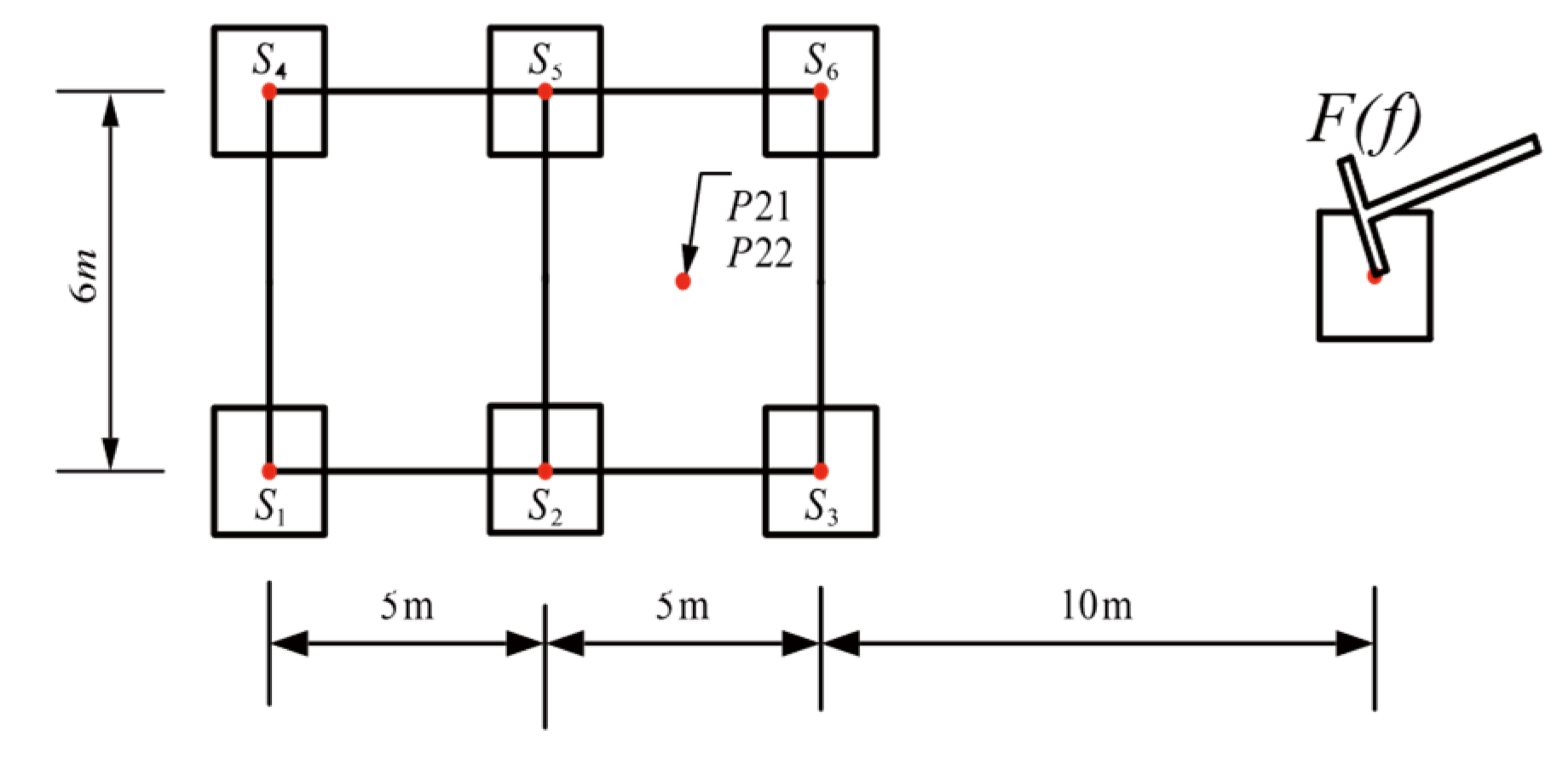
A three-story building is planned to be built near the train track. The building is a frame structure, with each layer 3.0 m high and a total of 9 m. The building layout is shown in Figure 4. The room size is 4.0 m × 6.0 m, the total width of the building is 8.0 m, and the total length is 12.0 m. The section dimensions of columns in the building are unified 400 mm × 400 mm; the thickness of each floor is about 0.1 m; and the building foundation size is 1.5 m × 1.5 m × 0.6 m. The building size parameters and load arrangements are shown in Figure 5.
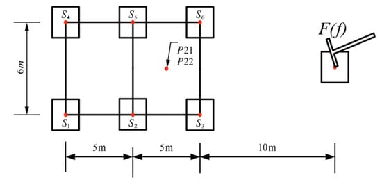
Figure 4.
Floor plan of the building.
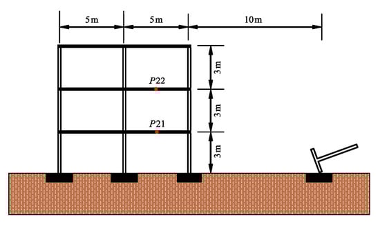
Figure 5.
Elevation of building layout.
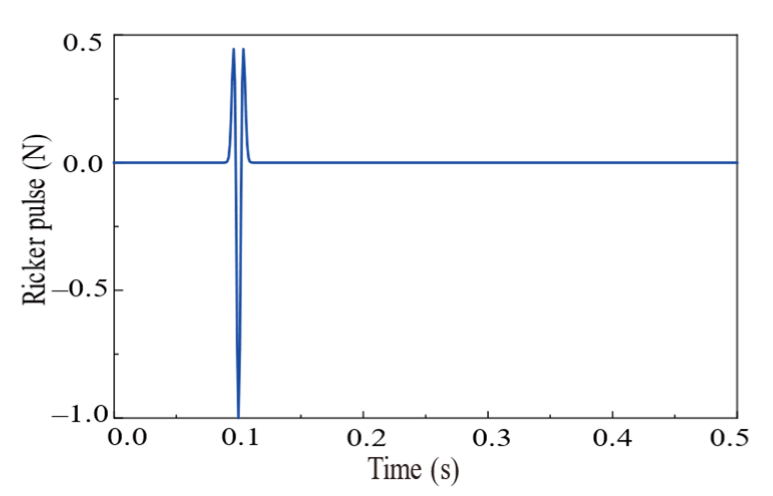
The expression in the time domain of Ricker pulse is:
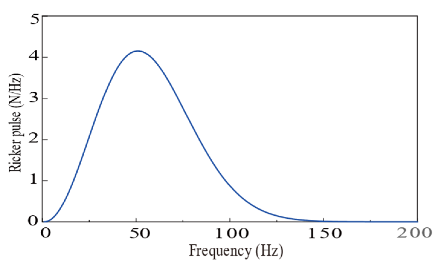
where ts = 0.1s, and TR = 0.01s. The time-domain and frequency-domain representations of the Ricker pulse are displayed in Figure 6 and Figure 7, respectively.

Figure 6.
Time domain diagram of Ricker pulse.

Figure 7.
Frequency domain diagram of Ricker pulse.
The free-field displacement curve, , at the building foundation under the action of Ricker pulse is shown in Figure 8.
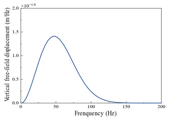
Figure 8.
Vertical free-field displacement curve at S2 of the building foundation under the action of Ricker pulse.
The building’s geometric dimensions, material properties, and structural parameters are input into a MATLAB (R2019b) program to compute the overall characteristic matrix of the node-based building. The floor amplification factor is subsequently derived using Equation (33). The results are displayed in Figure 9.
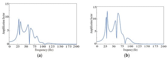
Figure 9.
Magnification factor of each floor. (a) The second floor of the building. (b) The third floor of the building.
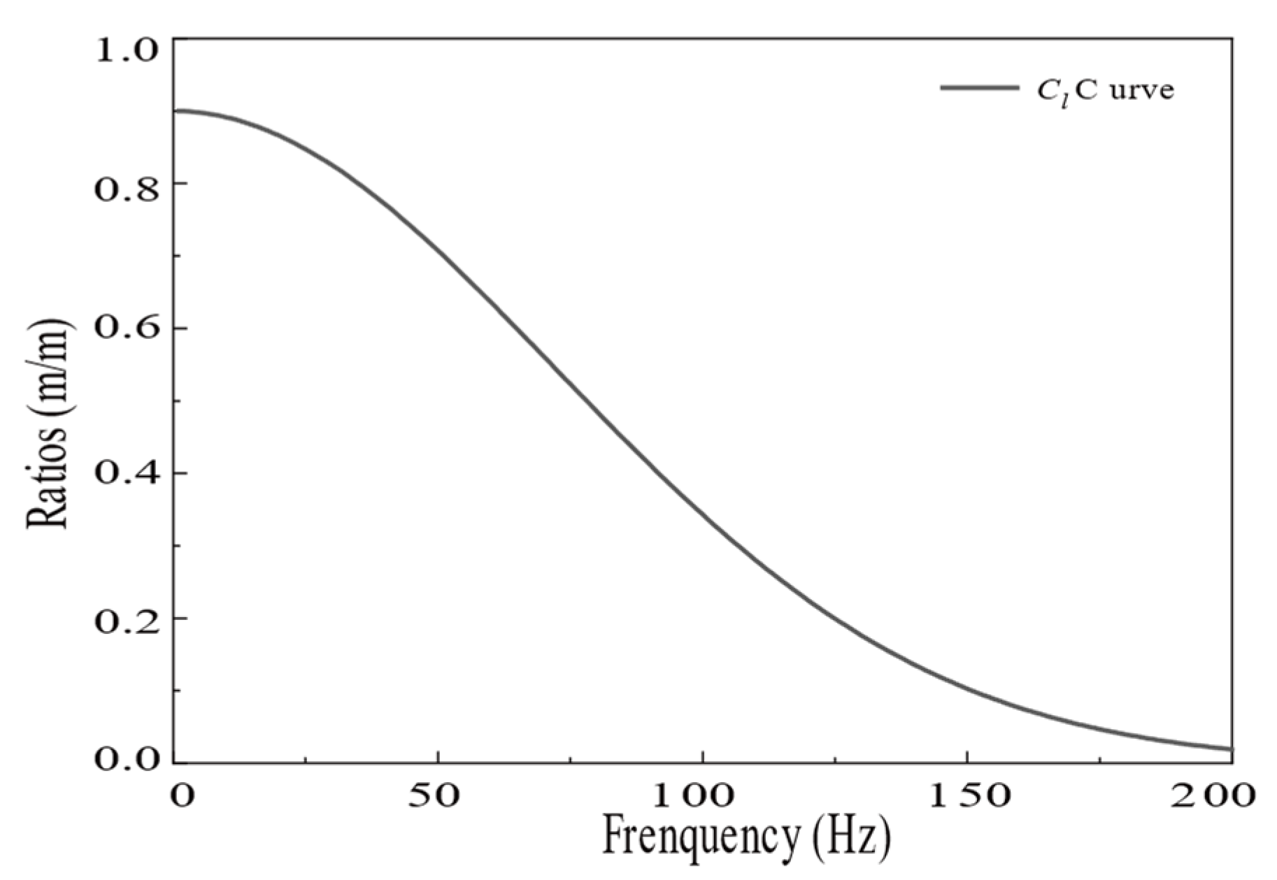
The saturated soil half-space model is simplified to a single elastic half-space by setting n, pf, b to values near zero (0.0001 in this study). Other parameters are kept consistent with Colaco et al. [19]. In conclusion, the coupling loss coefficient curve was obtained as shown below (Figure 10).
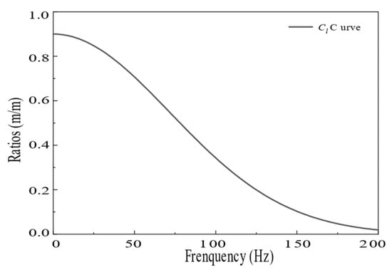
Figure 10.
Coupling loss coefficient curve.
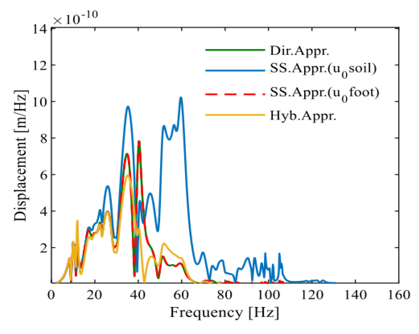
The vertical vibrations induced by a Ricker pulse in a saturated half-space, the coupling loss coefficient reflecting the interaction between saturated soil and foundation, and the floor amplification system derived in this section can be incorporated into Equation (3) to determine the vibration response of each building floor, depicted in Figure 11 and Figure 12. By comparing the calculated results with those of Colaco, the red dotted lines in Figure 13 and Figure 14 are the response curves of each floor calculated after considering SSI in the reference [19].
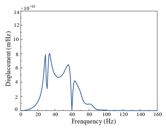
Figure 11.
The vertical displacement of the second floor of the building obtained by the soil–structure transfer function method.
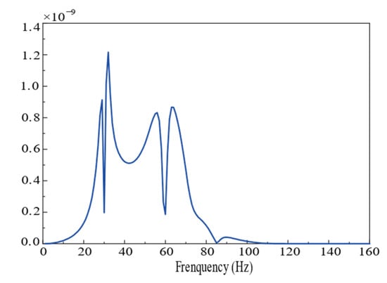
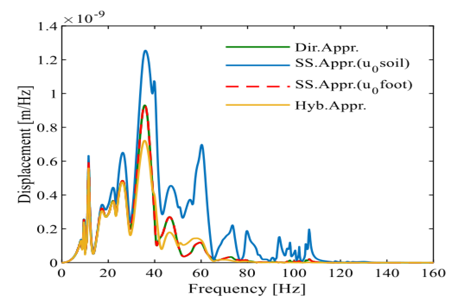
Figure 12.
The vertical displacement of the floor slab of the third floor of the building obtained by the soil–structure transfer function method.
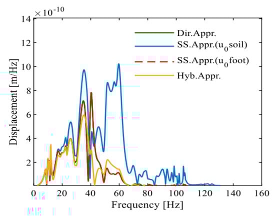
Figure 13.
The vertical displacement of the second floor slab of a building obtained by Colaco et al. [19].
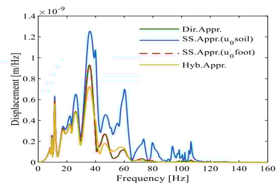
Figure 14.
Vertical displacement of three-story floor slab of a building obtained by Colaco et al. [19].
It can be observed that the calculated results at 50~70 Hz are larger than those by Colaco et al. [19], which is caused by the difference in free-field vibration. The peak frequency of free-field vibration calculated in this section is around 50 Hz, so the vibration of the building is amplified in this frequency band. The findings of this study are compared with those of Colaco, and the results show a reasonable level of agreement in terms of amplitude, curve series, and peak frequency localization. In structural engineering, a common criterion for model validation is an error margin of 5%, as used in FEM updating based on Operational Modal Analysis [32]. Applying this benchmark, the percentage error in our results compared to Colaco’s findings falls within an acceptable range, supporting the validity of our proposed method.
4. Conclusions
This study proposes an analytical transfer function method to predict building vibrations induced by external loads on saturated foundation soils. The method integrates Rayleigh wave propagation, coupling loss coefficients, and floor amplification effects into a unified framework, effectively addressing limitations in existing numerical and experimental approaches. The main findings and contributions are as follows:
- The coupling loss coefficient, derived from Rayleigh wave reflection and transmission theory, quantifies the interaction intensity between saturated soil and building structures. It depends on the material properties and load frequency, offering a robust analytical solution. The floor amplification coefficient, derived from the structural dynamics equation, reflects the dynamic response of individual building floors. The results reveal that higher floors experience greater amplification, with the peak amplification frequency corresponding to the building’s natural vibration frequency.
- The method’s predictions align closely with results from existing numerical and experimental studies, particularly in saturated soil conditions. Its ability to capture key vibration characteristics while reducing computational complexity demonstrates its practical applicability. The proposed method provides an efficient and generalizable tool for vibration analysis in engineering applications.
- The method is particularly suited for scenarios involving small-to-medium amplitude vibrations, such as traffic-induced vibrations near railways, highways, or subways. Its predictive capabilities can guide the design of vibration mitigation strategies, optimize isolation systems, and assess the environmental impact of infrastructure projects. While the method assumes linear soil–structure interactions, future work could extend it to include nonlinear dynamics for applications in high-intensity scenarios, such as earthquakes or explosions.
In conclusion, the transfer function method represents a significant advancement in SSI research, offering both theoretical innovation and practical solutions. By bridging the gap between empirical and numerical methods, it lays the groundwork for further developments in vibration prediction and mitigation, particularly in complex urban environments. The findings of this study not only validate the feasibility of the proposed method but also highlight its potential for widespread engineering applications.
Author Contributions
Conceptualization, J.Y. and N.W.; methodology, J.Y.; software, Y.C.; validation, J.Y., N.W. and Y.C.; formal analysis, J.Y.; investigation, N.W.; resources, J.Y.; data curation, Y.C.; writing—original draft preparation, N.W.; writing—review and editing, J.Y.; visualization, Y.C.; supervision, J.Y.; project administration, J.Y.; funding acquisition, J.Y. All authors have read and agreed to the published version of the manuscript.
Funding
This research was financially supported by the National Natural Science Foundation of China (52472320).
Data Availability Statement
Data are openly available in a public repository.
Conflicts of Interest
The authors declare no conflicts of interest.
References
- Xia, H.; Wu, X.; Yu, D. Environment Vibration Induced by Urban Rail Transit System. J. North. Jiaotong Univ. 1999, 23, 1–7. [Google Scholar]
- Coulier, P.; Lombaert, G.; Degrande, G. The influence of source—Receiver interaction on the numerical prediction of railway induced vibrations. J. Sound Vib. 2014, 333, 2520–2538. [Google Scholar] [CrossRef]
- Francois, S.; Pyl, L.; Masoumi, H.R.; Degrande, G. The influence of dynamic soil structure interaction on traffic induced vibrations in buildings. Soil Dyn. Earthq. Eng. 2007, 27, 655–674. [Google Scholar] [CrossRef]
- Xia, H.; Zhang, N.; Cao, Y. Experimental Study of Train-induced Vibrations of Ground and Nearby Buildings. J. China Railw. Soc. 2004, 26, 93–98. [Google Scholar] [CrossRef]
- Cao, Y. Theoretical Analysis and Experimental Study on Free Field and Building Vibration Caused by Trains; Beijing Jiaotong University: Beijing, China, 2006. [Google Scholar]
- Sanayei, M.; Maurya, P.; Moore, J.A. Measurement of building foundation and ground-borne vibrations due to surface trains and subways. Eng. Struct. 2013, 53, 102–111. [Google Scholar] [CrossRef]
- Galvin, P.; Dominguez, J. Experimental and Numerical Analyses of Vibrations Induced by High-speed Trains on the Cordobamalaga Line. Soil Dyn. Earthq. Eng. 2009, 29, 641–657. [Google Scholar] [CrossRef]
- Connolly, D.; Kouroussis, G.; Woodward, P.; Costa, P.A.; Verlinden, O.; Forde, M. Field Testing and Analysis of Highspeed Rail Vibrations. Soil Dyn. Earthq. Eng. 2014, 67, 102–118. [Google Scholar] [CrossRef]
- Zhai, W.M.; Wei, K.; Song, X.L. Experimental Investigation into Ground Vibrations Induced by Very Highspeed Trains on A Non-ballasted Track. Soil Dyn. Earthq. Eng. 2015, 72, 24–36. [Google Scholar] [CrossRef]
- Madshus, C.; Bessason, B.; Harvik, L. Prediction Model for Low Frequency Vibration from High Speed Railways on Soft Ground. J. Sound. Vib. 1996, 193, 195–203. [Google Scholar] [CrossRef]
- Sadeghi, J.; Vasheghani, M. Safety of Buildings against Train induced Structure Borne Noise. Build. Environ. 2021, 197, 107784. [Google Scholar] [CrossRef]
- Farahani, M.V.; Sadeghi, J.; Jahromi, S.G.; Sahebi, M.M. Modal based method to predict subway train-induced vibration in buildings. Structures 2023, 47, 557–572. [Google Scholar] [CrossRef]
- Sadeghi, J.; Vasheghani, M. Improvement of Current Codes in Design of Concrete Frame Buildings: Incorporating Train-induced Structure Borne Noise. J. Build. Eng. 2022, 58, 104955. [Google Scholar] [CrossRef]
- Yao, J.B. Research on Environmental Vibration and Isolation Measures Caused by Rail Transit Considering Soil Structure Dynamic Interaction; Beijing Jiaotong University: Beijing, China, 2010. [Google Scholar]
- Lei, F. Research on Prediction Method of Environmental Vibration Caused by High-Speed Train Based on Random Forest Algorithm; Beijing Jiaotong University: Beijing, China, 2020. [Google Scholar]
- Rucker, W.; Auersch, L. A User-friendly Prediction Tool for Railway Induced Ground Vibrations: Emission—Transmission—Immission. In Notes on Numerical Fluid Mechanics and Multidisciplinary Design; Springer: Berlin/Heidelberg, Germany, 2008; pp. 129–135. [Google Scholar]
- Auersch, L. Building Response Due to Ground Vibration-simple Prediction Model Based on Experience with Detailed Models and Measurements. Int. J. Acoust. Vib. 2010, 15, 101–112. [Google Scholar] [CrossRef]
- Vogiatzis, K. Protection of The Cultural Heritage from Underground Metro Vibration and Ground-borne noise in Athens Centre: The Case of the Kerameikos Archaeological Museum and Gazi Cultural Centre. Int. J. Acoust. Vib. 2012, 17, 59–72. [Google Scholar]
- Colaco, A.; Barbosa, D.; Costa, P.A. Hybrid Soil–structure Interaction Approach for the Assessment of Vibrations in Buildings Due to Railway Traffic. Transp. Geotech. 2022, 32, 100691. [Google Scholar] [CrossRef]
- Araz, O.; Elias, S.; Kablan, F. Seismic-induced Vibration Control of A Multistory Building with Double Tuned Mass Dampers Considering Soil–structure Interaction. Soil Dyn. Earthq. Eng. 2023, 166, 107765. [Google Scholar] [CrossRef]
- Kanellopoulos, C.; Rangelow, P.; Jeremic, B.; Anastasopoulos, I.; Stojadinovic, B. Dynamic Structure–Soil–structure Interaction for Nuclear Power Plants. Soil Dyn. Earthq. Eng. 2024, 181, 108631. [Google Scholar] [CrossRef]
- Colaco, A.; Costa, P.A.; Castanheira-Pinto, A.; Amado-Mendes, P.; Calcada, R. Experimental Validation of a Simplified Soil–Structure Interaction Approach for the Prediction of Vibrations in Buildings Due to Railway Traffic. Soil Dyn. Earthq. Eng. 2021, 141, 106499. [Google Scholar] [CrossRef]
- Kuo, K.A.; Papadopoulos, M.; Lombaert, G.; Degrande, G. The Coupling Loss of a Building Subject to Railway Induced Vibrations: Numerical Modelling and Experimental Measurements. J. Sound Vib. 2019, 442, 459–481. [Google Scholar] [CrossRef]
- Lapez-Mendoza, D.; Connolly, D.P.; Romero, A.; Kouroussis, G.; Galvin, P. A Transfer Function Method to Predict Building Vibration and Its Application to Railway Defects. Constr. Build. Mater. 2020, 232, 117217. [Google Scholar] [CrossRef]
- Yao, J.B.; Wu, Z.Z.; Cao, X.F. Derivation and Application of Analytical Coupling Loss Coefficient by Transfer Function in Soil–Building Vibration. Buildings 2024, 14, 1933. [Google Scholar] [CrossRef]
- Lapwood, E.R. The Transmission of a Rayleigh Pulse Round a Corner. Geophys. J. R. Astron. Soc. 1961, 4, 174–196. [Google Scholar] [CrossRef]
- Maurice, J.Y. The Reflection and Transmission of Rayleigh Waves; University of British Columbia: Vancouver, BC, Canada, 2012; Volume 112, p. 103520. [Google Scholar] [CrossRef]
- Yao, J.B.; Zhao, R.T.; Zhang, N.; Yang, D.J. Vibration Isolation Effect Study of In-filled Trench Barriers to Train-induced Environmental Vibrations. Soil Dyn. Earthq. Eng. 2019, 125, 105741. [Google Scholar] [CrossRef]
- Ditommaso, R.; Mucciarelli, M.; Ponzo, F.C. Analysis of Non-stationary Structural Systems by Using a Band-variable Filter. Bull. Earthq. Eng. 2012, 10, 895–911. [Google Scholar] [CrossRef]
- Xia, T.D.; Chen, L.Z.; Wu, S.M. Characteristics of Rayleigh Waves in Half Space Saturated Soil. J. Hydraul. Eng. 1998, 2, 7–11. [Google Scholar]
- Oñate, E. Thin Plates. Kirchhoff Theory. In Structural Analysis with the Finite Element Method Linear Statics; Lecture Notes on Numerical Methods in Engineering and Sciences; Springer: Dordrecht, The Netherlands, 2013. [Google Scholar]
- Alpaslan, E.; Hacefendiolu, K.; Demir, G.; Birinci, F. Response Surface-based Finite-element Model Updating of a Historic Masonry Minaret for Operational Modal Analysis. Struct. Des. Tall Spec. Build. 2020, 29, e1733. [Google Scholar] [CrossRef]


Disclaimer/Publisher’s Note: The statements, opinions and data contained in all publications are solely those of the individual author(s) and contributor(s) and not of MDPI and/or the editor(s). MDPI and/or the editor(s) disclaim responsibility for any injury to people or property resulting from any ideas, methods, instructions or products referred to in the content. |
© 2025 by the authors. Licensee MDPI, Basel, Switzerland. This article is an open access article distributed under the terms and conditions of the Creative Commons Attribution (CC BY) license (https://creativecommons.org/licenses/by/4.0/).