A Numerical Study on the Utilization of Small-Scale Model Testing for Slope Stability Analysis

Abstract

Small-scale model tests have been used widely to examine the behavior of slopes. When all similarity principles are conformed, the test results can be translated to the behaviors of slopes in the prototype. However, when the similarity principles cannot be fully conformed, the model test results need to be interpreted. The interpretation of the slopes stability behaviors from the small-scale model test under non-conformity conditions to that of the prototype is investigated, considering various slope scales and soil properties, undertaken through the finite element (FE) method conducted by the ABAQUS package. Prior to conducting the finite element (FE) parametric study, the numerical results were verified by comparing them with data from previous studies, with good agreement obtained. According to the findings from the parametric study, a framework was developed to allow the 1 g model-scale test results to be translated to the parameters used for the prototype slope design. The study examined both the sliding surfaces and the safety factors of slopes to establish a connection between model tests and their full-scale counterparts. This framework provides a means to effectively utilize 1 g of small-scale test data for designing and analyzing prototype slopes.

1. Introduction

1.1. Reduced Scale Model Test

Slope stability is a classical problem in geotechnical engineering design. In addition to the conventional analytical methods to assess its stability with relatively uniform soils, such as slip circle, the methods of slices, and FEM methods [1,2,3,4,5], model tests have been used broadly to explore the slope stability with relatively complex soils (i.e., layered soils) [6,7,8,9]. Due to the large geometrical dimensions of slopes in the prototype, reduced-scale model tests, such as centrifuge tests and small-scale model (i.e., 1 g) tests, are commonly used to explore the failure mechanisms of slopes and evaluate slope stability in the laboratory by researchers [10,11,12,13,14,15,16]. The prototype stress conditions can be simulated in centrifuge tests by lifting centrifugal acceleration. This, of course, depends on the availability of the centrifuge facility. Compared to the high cost of centrifuge equipment, conventional gravity model tests are efficient and affordable.

For conventional reduced-scale model tests, to accurately represent the characteristics of the slope, the similarity principles [17] must be satisfied. The dimensions of the slope in the 1 g model test are reduced to a certain size, and the properties of soils should also be adjusted accordingly following the similarity principle, taking the geometry conversion coefficient C_L = n, the stress conversion coefficient of C_σ = n, and the modulus conversion coefficient of C_E = n. In addition, there are other similarity coefficients required, as shown in

Table 1. Summary of main conversion coefficients of similarity principle.

Conversion Coefficients	Notation	Expression **	Value
Geometry conversion coefficient	CL	Lp/Lm	n
Unit weight conversion coefficient	Cγ	γp/γm	1
Poisson’s ratio conversion coefficient	Cυ	υp/υm	1
Stress conversion coefficient	Cσ	σp/σm	n
Modulus conversion coefficient	CE	Ep/Em	n
Internal friction angle conversion coefficient	Cφ	φp/φm	1

** The reduced scale is assumed to be n. The subscript of ‘p’ and ‘m’ represent ‘prototype’ and ‘model’, respectively.

. The similarity principle formed by these coefficients is designed to ensure that the model test slope exhibits the same behavior as that in the prototype. When the dimensions of the model are reduced, the soil strength must also be proportionally decreased. It is no problem to conform to the geometry similarity during the model preparation. However, to conform, the similarity of the material properties, the soil strength must also be reduced correspondingly. Therefore, the soil strength in the small-scale test must be kept at a very low level to follow the similarity principle. This implies that, when the scaling factor is n (i.e., L_prototype/L_model = n), the soil strength must be reduced according to the ratio s_u-prototype/s_u-model = n. For instance, if n = 50 and s_u-prototype = 25 kPa, then s_u-model would need to be 25 kPa/50 = 0.5 kPa. Preparing a soil sample with such low shear strength to accurately replicate the behavior of natural soil is extremely challenging (especially for clay) in a reduced-scale model [7,11,18]. Without following the similarity principles for small-scale model tests, the slope behavior in the scale model test cannot be translated to the slope behavior in the prototype slopes directly. This constrains the use of small-scale model tests for evaluating slope behavior in prototypes. In scale model tests that do not adhere to similarity principles, the model slope’s stability is consistently higher than that of the prototype slope. This is due to the difficulty in preparing soil with the necessary low strength, as explained earlier. Consequently, the sliding surface cannot be directly observed, and the model slopes do not collapse during the testing. Some measures were adopted to make model slopes collapse in scale model tests. The slope angle rotation system was a normal measure, which made model slopes collapse by increasing the slope angle of the model [19]. Slope cut was also a common measure used in centrifuge tests and scale model tests, which make model slopes collapse by decreasing the slope angle of the model [13,20].

1.2. Previous Work

Numerous studies have been conducted to provide insight into the behavior of slopes through reduced scale model tests, including (i) the study of the static and dynamic stability of wedge blocks and slopes, in which the limiting equilibrium approach, based on the sliding surface obtained from the model test, was used to predict the safety factor of the slope [21,22]; (ii) the effect of water pressures on the stability of the slope [23,24]; (iii) the behavior of the slope under rainfall loading [10]; and (iv) the effect of loading magnitude and slope angle [11].

Lin et al. (2015) [11] proposed a new reduced-scale model testing method to evaluate slope safety factors. In their tests, the slope was constructed on a flat testing bed that can be rotated by hydraulic lifts. By increasing the rotation angle of the testing bed, the gravitational force component driving slope sliding was increased, hence triggering the slope to fail. A method for predicting the safety factor of the slope was proposed based on the displacement data from the model test.

Finite element methods combined with centrifuge tests are used to investigate the effect of gravity acceleration levels (g-level) on the slope stability by many researchers [25,26,27,28,29]. Yang et al. (2012) [26] observed that as the g-level increases in centrifuge testing, the slope stability significantly decreases. Notably, for a model slope in a centrifuge test, the factor of safety (F_s) shifted from stable to failure, dropping from 2 to 1 as the g-level increased from 10 to 50. Therefore, the slopes with the same shape and in situ strength can behave quite differently when their geometry scale increases proportionally.

Based on the previous work on slope stability studies, it can be seen that, although a 1-g model test is a convenient and economical way to test slope stability, there are two obstacles: (a) it is difficult to set up a small-scale model test that conforms to all similarity rules at the same time (i.e., geometry similarity and material similarity), especially for the case of a soft foundation; (b) the slope behavior changes with changing slope geometry scale when soil strength is kept at its in-situ value. Previous studies rarely discussed the specific impacts of non-compliant similarity coefficients on test results when the scaled physical model does not fully satisfy the similarity principle because they generally used the results without following the similarity principle to do qualitative analysis for the failure mechanism of the slope, with a qualitative understanding of the failure mechanism of the slope. Furthermore, it is quite hard to find some reported correction methods for the experimental deviations caused by such similarity discrepancies.

1.3. Objective of Present Study

This study investigates the application of scaled model tests in slope stability analysis, with a particular focus on scaled model tests that do not fully comply with the similarity principles. Given the challenges in fully replicating these similarities in small-scale tests, numerical analysis proves useful in examining the effects of these similarities and differences. As a widely applied numerical method, the finite element method (FEM) is very convenient and powerful for quantitatively evaluating slope stability. It can simulate and analyze various working conditions and parameter combinations to study the impact of potential influencing factors on the performance of the slope in scaled model tests. This approach helps to connect the results of small-scale tests to the performance of prototype slopes.

2. Parametric Study Set Up

The numerical FE software ABAQUS (6.11) [30] is chosen to investigate the potential failure mechanisms and safety factor of the slope with uniform strength. After the validation of the FE analysis against existing published data, a series of parametric studies is conducted to explore the failure mechanisms and corresponding safety factors of the slope to estimate its stability.

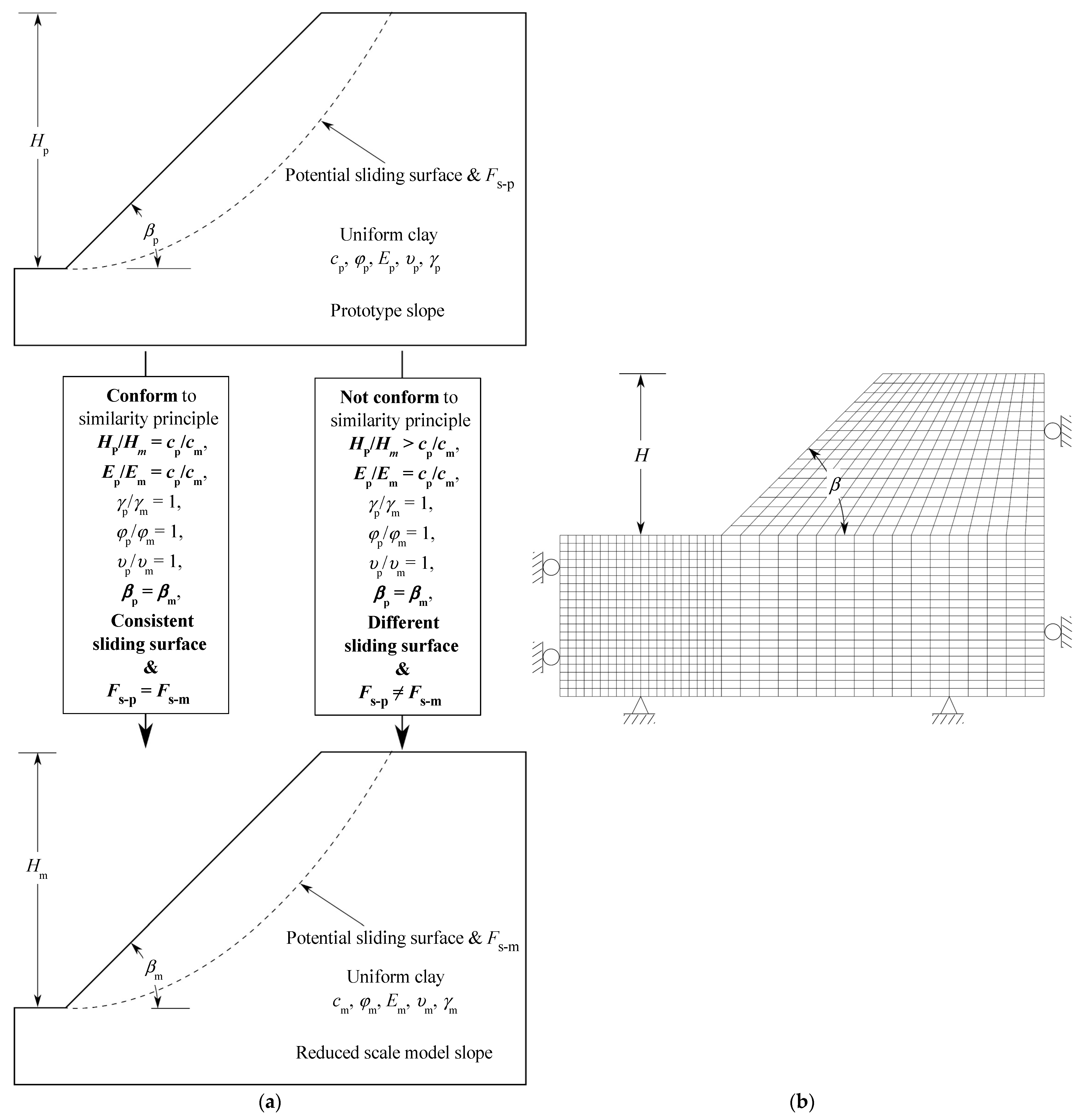
2.1. Finite Element Model

The finite element method with shear strength reduction (SSR) is used to analyze the slope stability in this study due to its extensive application [3,31,32,33,34]. A two-dimensional analysis under plane strain conditions in finite element software ABAQUS [30], depicted in Figure 1, is used to assess the stability of the slope. The model’s side boundaries are allowed to move vertically, but horizontal displacement is restricted, while the bottom boundary is fully fixed, preventing both vertical and horizontal movements. The slope is simulated under undrained conditions, using 4-node bilinear plane strain quadrilateral elements with reduced integration. The typical finite element mesh used for the slope model in this study is also illustrated in Figure 1b.

2.2. Material Model and Parameters

A linear elastic-perfectly plastic material is used to model the slope following the Mohr–Coulomb failure criterion with five key parameters: c, φ, ψ, E, and υ. The parameters used in this study are detailed in

Table 2. Summary of FE analyses performed on uniform slope: stability analysis.

Analysis	cp (kPa)	φ (°)	β (°)	Hp (m)	CL	Cc	Notes
Group I	12.38	20	45	10	1	1	Validation against Dawson et al. (1999) [3]
Group II	10	20	26.57	10	1	1	Validation against Griffiths and Lane (1999) [4]
Group III	10, 20, 30, 40, 50	20	45	10	1	1	Investigation of the effect of cp, φ, β, and Hp on the stability of the prototype slope
	20	10, 30, 40, 50	45	10
	20	20	15, 30, 60, 75	10
	20	20	45	2.5, 5, 20, 30, 40, 50
Group IV	10, 20, 30, 40, 50	20	45	10	2.5, 5, 7.5, 10	1, 2.5, 5, 7.5, 10	Investigation of the effect of cp on the stability of the model slope
Group V	20	10, 30, 40, 50	45	10	2.5, 5, 7.5, 10	1, 2.5, 5, 7.5, 10	Investigation of the effect of φ on the stability of the model slope
Group VI	20	20	15, 30, 60, 75	10	2.5, 5, 7.5, 10	1, 2.5, 5, 7.5, 10	Investigation of the effect of β on the stability of the model slope
Group VII	20	20	45	20, 30, 40, 50	2.5, 5, 7.5, 10, 15, 20, 25, 30, 35, 40, 45, 50	1, 2.5, 5, 7.5, 10, 15, 20, 25, 30, 35, 40, 45, 50	Investigation of the effect of Hp on the stability of the model slope

. In the study, three parameters are maintained at constant values, such as Poisson’s ratio (υ = 0.3) [4], the ratio of Young’s modulus to cohesion (E/c = 500) [8,35], and dilatancy angle (ψ = 0).

Under the Mohr–Coulomb failure criterion, the shear strength is represented as

$$\tau =c+{\sigma }_n\tan \phi$$

(1)

Using the SSR technique, the shear strength is reduced by lowering the values of the two shear strength parameters, namely,

$$c_{SSR}=c/F_{SSR}$$

(2)

$${\phi }_{SSR}=\arctan (\tan \phi /F_{SSR})$$

(3)

Here, F_SSR represents the strength reduction factor associated with the shear strength parameters. In prior research on slope stability [2,36], the factor of safety F_s is traditionally defined as the ratio of the actual shear strength of the soil (i.e., c and φ) to the minimum shear strength needed to prevent failure (i.e., $c_{SSR}^f$ and ${\phi }_{SSR}^f$). This is,

$$F_s=F_{SSR}^f={\displaystyle \frac{c}{c_{SSR}^f}}={\displaystyle \frac{\tan \phi }{\tan {\phi }_{SSR}^f}}$$

(4)

2.3. Conversion Coefficients

Small-scale slope model test is a branch of the geological mechanical model test. The geological mechanical model test must satisfy three similitudes: geometry, loading, and material properties [7]. Geometric similitude is achieved when the model is geometrically similar to the prototype. The type of loading applied must resemble that experienced by the prototype and should be proportional in magnitude. Additionally, the stress-strain characteristics of the model material are needed to match those of the prototype material within the stress range of the test. The main form of a small-scale model test is a frame model test, which can follow the geometry similarity principle and use the same type of material with the same or different properties. In terms of geometrical dimensions, the prototype slope is significantly large in width and height for the real project of the slope. However, the laboratory’s size is often very small compared to the dimensions of the prototype. The small-scale model of a slope needs to be designed, ideally, to follow all similitudes [17], where the physical dimensions and material mechanical behaviors are reduced with the same ratio. The primary conversion coefficients of the similarity principles are summarized in Table 1 as the reduced scale of geometry is n.

Before delving into the analysis, several assumptions are outlined. In small-scale model tests without frictional boundaries, the conversion coefficients primarily involve geometry, physical properties, mass, and load conversions. In this study, the reduced scale of model tests is expressed in terms of the geometry conversion coefficient (i.e., C_L = n). The conversion coefficients for internal friction angle, Poisson’s ratio, strain, and unit weight are set as a constant, C_φ = C_ε = C_γ= C_υ = 1 (refer to Table 1).

The cohesion conversion coefficient (C_c) is another key parameter. When setting up a model test, the value of C_c is typically smaller than the value of C_L (i.e., C_c < C_L = n) due to the difficulty in preparing low-strength soil. In other words, the soil strength in the model test cannot be too low, as this would make the slope behavior unrealistic or impractical.

In this parametric analysis, the cohesion conversion coefficient (C_c) is set equal to the modulus conversion coefficient (C_E) according to the above, E/c = 500. Therefore, the parameters of the numerical model can be controlled by two variables, C_L and C_c. The numerical case studies are designed to explore the impact of varying these two coefficients on slope performance. The parameter ranges used in the numerical case studies are provided in Table 2.

3. Validation of FE Analysis

Two case studies are included in the validation analysis. Case 1 was studied by Dawson et al. (1999) [3] using the finite difference method. Case 2 was examined by Griffiths and Lane (1999) [4] using the finite element method. Both studies assume two initial pore water pressures, meaning that the total and effective stresses are identical.

Case 1, as shown in Figure 2a, is a homogeneous slope with the height of H = 12 m, the slope angle of β = 45°, and the foundation soil of a 2-m thick layer. Under the same conditions and the same setting of parameters, the finite element results of this study match the results from both finite difference and limit analyses as reported by Chen (1975) [37] and Dawson et al. (1999) [3].

Case 2, as shown in Figure 2b, is a homogeneous slope with a slope angle of β = 26.57^o (slope ratio of 2:1) and no foundation soil layer. In addition, the internal friction angle of the slope soil is 20° and c/γH = 0.05. As depicted in Figure 2b, the results of Griffiths and Lane (1999) [4] and this study, including the factor of safety and failure mechanism, are very close.

Based on the results from both validation studies, it can be concluded that the finite element model established is suitable for the current investigation.

4. Results and Discussion

Parametric analyses were set up to study the effects of influencing factors on slope performance. These factors include (i) the soil strength parameters, c and φ; and (ii) the slope geometry parameters, β and H. The selected parameters are grouped in Table 2, with the focus of each group listed in the column labeled “Notes”.

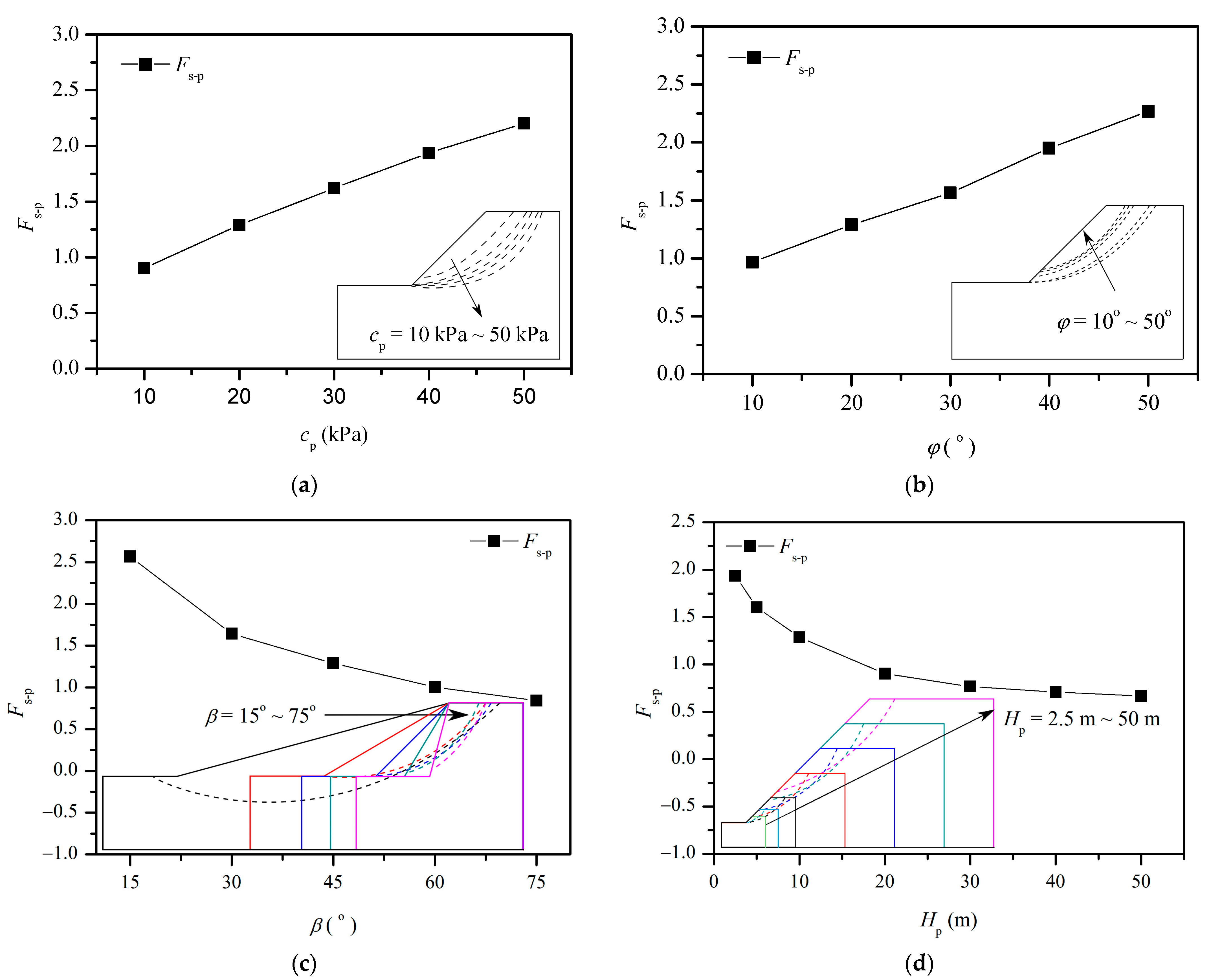
4.1. Effects of Four Influencing Factors on Prototype Slopes

To examine the impact of the four potential influencing factors (i.e., c, φ, β, and H) on the safety, soil flow mechanism, and sliding surface of a prototype slope, each group of cases is selected by varying only one parameter, while the other three parameters are held constant (Group III, Table 2).

Figure 3 shows the effects of the four parameters on the safety factor and the failure sliding surface of the slope in the prototype. It can be seen that the safety factor of the slope almost increases fairly linearly with the increasing soil shear strength c_p and friction angle φ as shown in Figure 3a,b. The slope failure surface is moving downwards with increasing soil shear strength c and decreasing soil friction angle φ. Hence, the area of shearing along the sliding surface increases accordingly. Consequently, the stability of the slope is enhanced as a large volume of soil needs to be mobilized. These observations were also reported by Cheng et al. (2007) [38] from FE analysis and by Gao et al. (2013) [39] from limit analysis. In these studies, the slope failure surface became shallower with increasing soil internal friction angle φ.

On the other hand, the increase in slope height H_p and slope angle β have significant negative effects on the sliding surface and the factor of safety of the slope. From Figure 3c,d, it can be seen that the safety factor of the slope in the prototype decreases with increasing slope height H_p and slope angle β. As the slope angle steepens in Figure 3c, the area of the sliding surface reduces. As all sliding surfaces for all the cases with β = 15~75° pass through or over the slope toe, the safety factor keeps reducing. However, as the slope height increases from H_p = 2.5 to 50 m, the sliding surface does not pass through the slope toe as H_p > 2.5 m. Hence, the safety factor of the slope converges to F_s-p = 0.75 as H_p becomes 50 m or more. The effects of slope angle and slope height on the stability of a homogenous slope were also examined using finite difference and limit analysis methods, reported by Dawson et al. (1999) [3] and Chen (1975) [37]. The same trends were found in their studies.

4.2. Parametric Study on Small-Scale Model Slopes

To investigate the impact of reduction coefficients on the safety factor and failure mechanism of a small-scale model slope, a range of reduction coefficients are chosen for the geometry conversion coefficient, specifically C_L = 1, 2.5, 5, 7.5, 10, 20, 30, 40, and 50. The corresponding cohesion conversion coefficients are chosen as C_c = 1, 1~2.5, 1~5, 1~7.5, 1~10, 1~20, 1~30, 1~40, and 1~50. The details of these study cases are provided in Group IV to Group VII in Table 2. While C_c equals C_L, the similarity principles are adhered to perfectly, meaning that the soil flow mechanism, sliding surface, and the factor of safety match exactly with those of the prototype slope. However, in practice, the condition of C_c = C_L cannot be guaranteed, and the influence of the unequal C_c and C_L needs to be investigated, which are discussed in the following subsections.

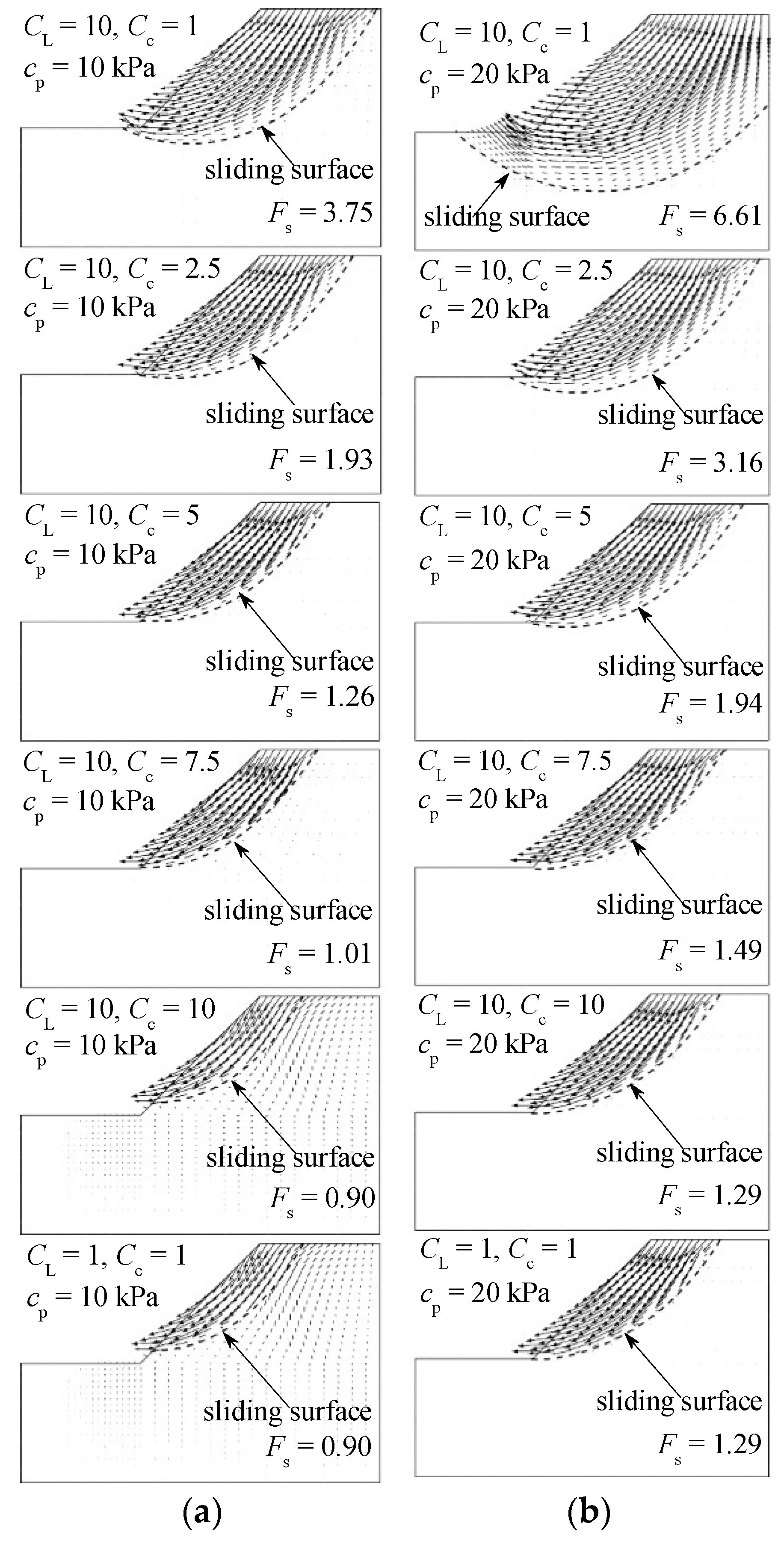
4.2.1. Effect of Model Scale with Varying Soil Cohesion

To investigate the impact of the reduction coefficient on the reduced-scale model test for soil cohesion, a set of cases is selected with varying prototype slope cohesion values (c_p = 10, 20, 30, 40, and 50 kPa), while keeping φ = 20°, β = 45°, and H_p = 10 m constant (Group IV, Table 2). The impact of the reduction coefficient on slope stability, as a function of cohesion, is shown in Figure 4. It is observed that when C_L = 10, the sliding surface contracts toward the slope shoulder as the cohesion conversion coefficient (C_c) increases from 1 to 10, with a corresponding decrease in the safety factor of the model slope. Comparing Figure 4a,b, it can be concluded that the influence of C_c on both the safety factor and sliding surface follows the same trend, regardless of the prototype cohesion values.

In order to examine the effect of the reduction coefficient on the stability of the reduced-scale model, the safety factors of the model slope by varying C_L and C_c are shown in Figure 5a,e. It is shown that the safety factor of the model slope, which conforms to the similarity principle (i.e., C_L = C_c) is equal to that of the prototype (i.e., C_L = C_c = 1) for different conversion coefficients. With the same geometry conversion coefficient, C_L, the safety factor of the model slope, F_s-m, decreases with increasing cohesion conversion coefficient, C_c. All trends in Figure 5a,e are similar for all prototype cohesions considered.

To check the effect of C_c/C_L on the safety factor, the safety factors of all cases are plotted in Figure 5f. It can be found that the safety factor of a model slope decreases with the increasing ratio of C_c/C_L. Moreover, the safety factor of the model slope converges to one of the prototype slopes at a given cohesion. This finding means that the ratio of C_c/C_L is an important parameter in reduced-scale model tests. The effect of the reduction coefficient on slope stability in the geotechnical model test was also reported by Chen et al. (2015) [7]. An equation about the similarity relation of the strength reduction safety coefficient was proposed in his study. It is stated that, with a constant geometry similarity factor (C_L), the safety factor (F_s) and the shear strength reduction coefficient (C_c) are inversely proportional. These results are also observed in this study, which shows that the safety factor decreases as C_c increases, given the same geometry conversion coefficient C_L.

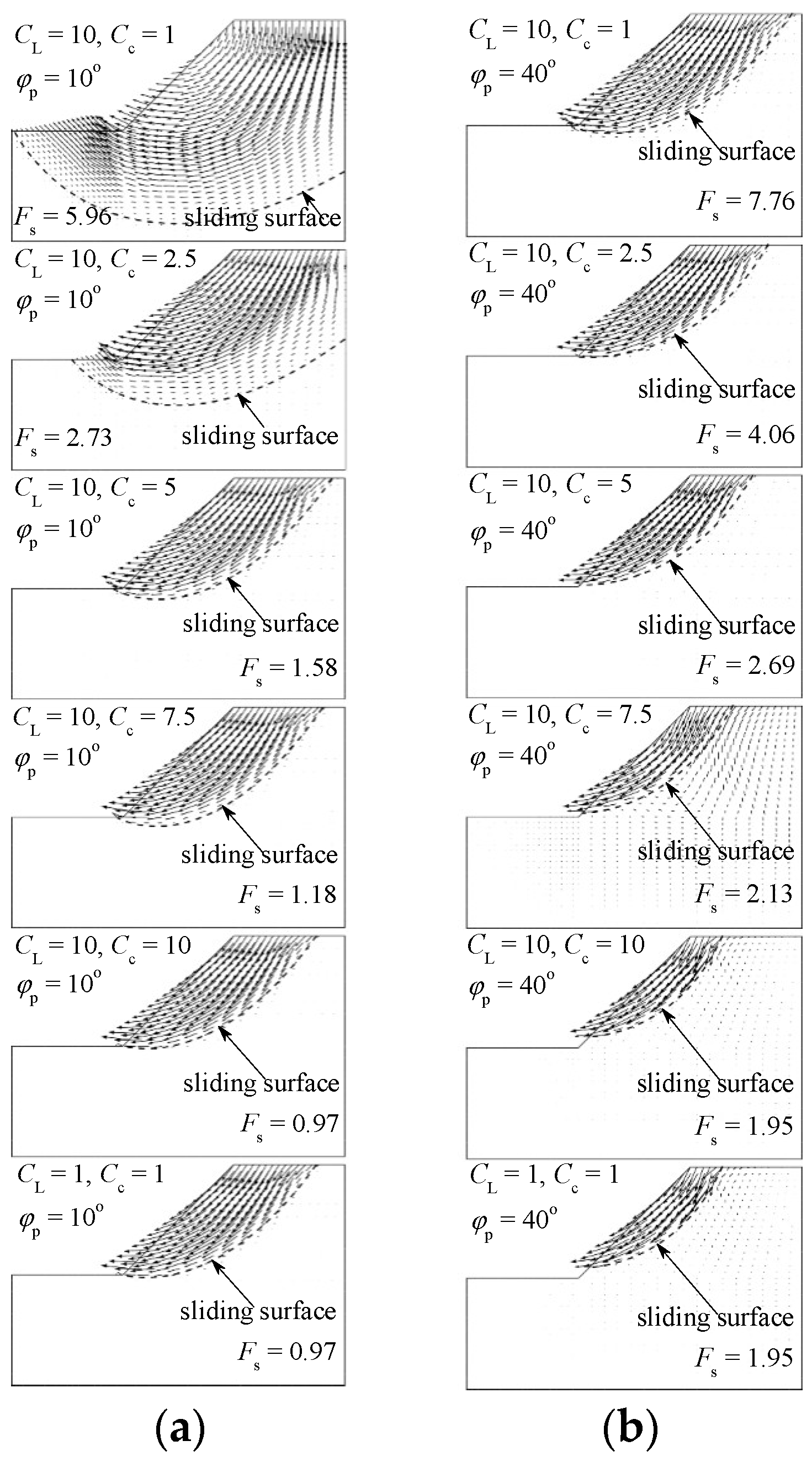
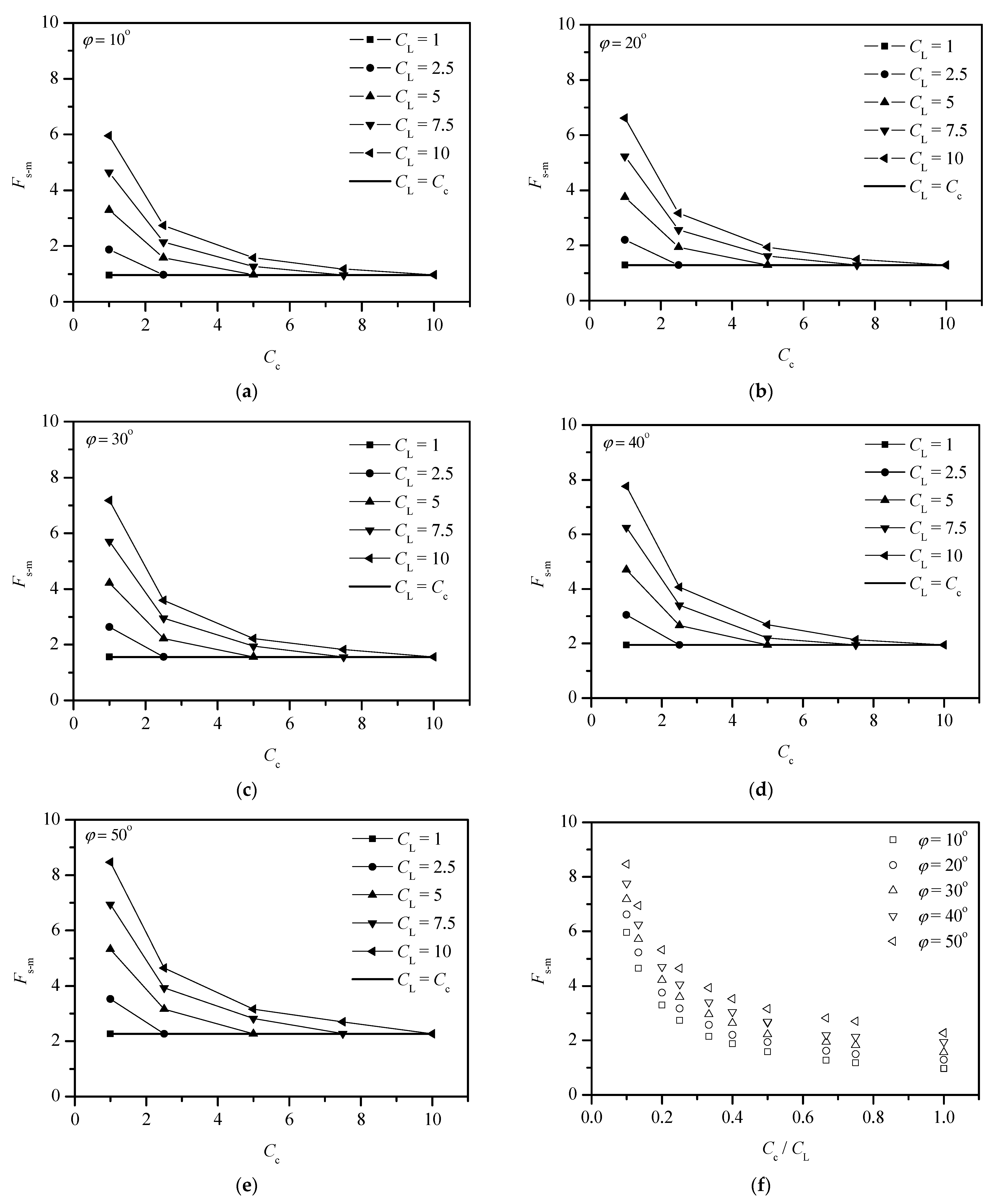
4.2.2. Effect of Model Scale with Varying Angle of Internal Friction

To analyze the effect of the reduction coefficient on slope stability by varying the internal friction angle, seventy cases are conducted with internal friction angles (φ) ranging from 10° to 50°, while keeping c_p = 20 kPa, β = 45°, and H_p = 10 m constant (Group V, Table 2). The failure mechanisms of the cases with φ = 10° and 40° are plotted in Figure 6. With the same geometry conversion coefficient C_L = 10, the sliding surface progressively shifts toward the slope shoulder, and the factor of safety gradually decreases as the cohesion conversion coefficient C_c increases from 1 to 10.

To check the effect of the reduction coefficient on slope stability by varying the internal friction angle, the safety factor of model slopes, F_s-m, versus conversion coefficients, C_L and C_c are plotted in Figure 7a,e for different internal friction angles. The shape of curves is similar for all cases, where F_s-m decreases with increasing C_c at a given C_L. All F_s-m curves converge to that of prototype slopes when C_L = C_c is reached.

Similar to the previous subsection of Figure 5f, the ratio of C_c/C_L is an important factor. The effect of C_c/C_L on the safety factor of a model slope for various internal friction angles is shown in Figure 7f. Same as Figure 5f, F_s-m decreases with increasing C_c/C_L, and converges to that of the prototype slope at C_c/C_L = 1.0. However, different from Figure 5f, F_s-m in Figure 7f decreases at a similar rate with increasing C_c/C_L for different φ.

The study of Yang et al. (2012) [26] illustrated the effect of g-level on the slope stability of the reduced scale model in the centrifuge test. Compared with the reduced-scale model tests under the condition of the 1-g model test, C_c = 1.0 is normally used for the case in the centrifuge test. Before acceleration begins, the geometry conversion coefficient (C_L) is set depending on the acceleration level of the test (n_t), resulting in C_c/C_L < 1.0. Once the centrifuge acceleration begins and increases to n, the equivalent C_Le decreases and equals C_L/n, causing the value of C_c/C_Le to increase. When the centrifuge acceleration reaches its target value (i.e., n = n_t), C_Le decreases until it equals C_c. Figure 5f and Figure 7f clearly illustrate that for a given c_p and φ, the safety factor of the model slope (F_s-m) is initially very high at low values of C_c/C_L. As C_c/C_L increases (corresponding to increasing acceleration level n), F_s-m decreases and eventually converges to the safety factor of the prototype slope (F_s-p) when C_c/C_L = 1.0, i.e., when the centrifuge reaches its target acceleration n_t.

In contrast, during a 1g model test, the geometry conversion coefficient C_L remains fixed. Reducing the soil’s shear strength to achieve C_c = C_L is not feasible, meaning that C_c/C_L will always be less than 1.0. Consequently, the factors of safety of 1 g model tests (F_s-m) will always be greater than that of the prototype slope (F_s-p), as shown in Figure 5 and Figure 7.

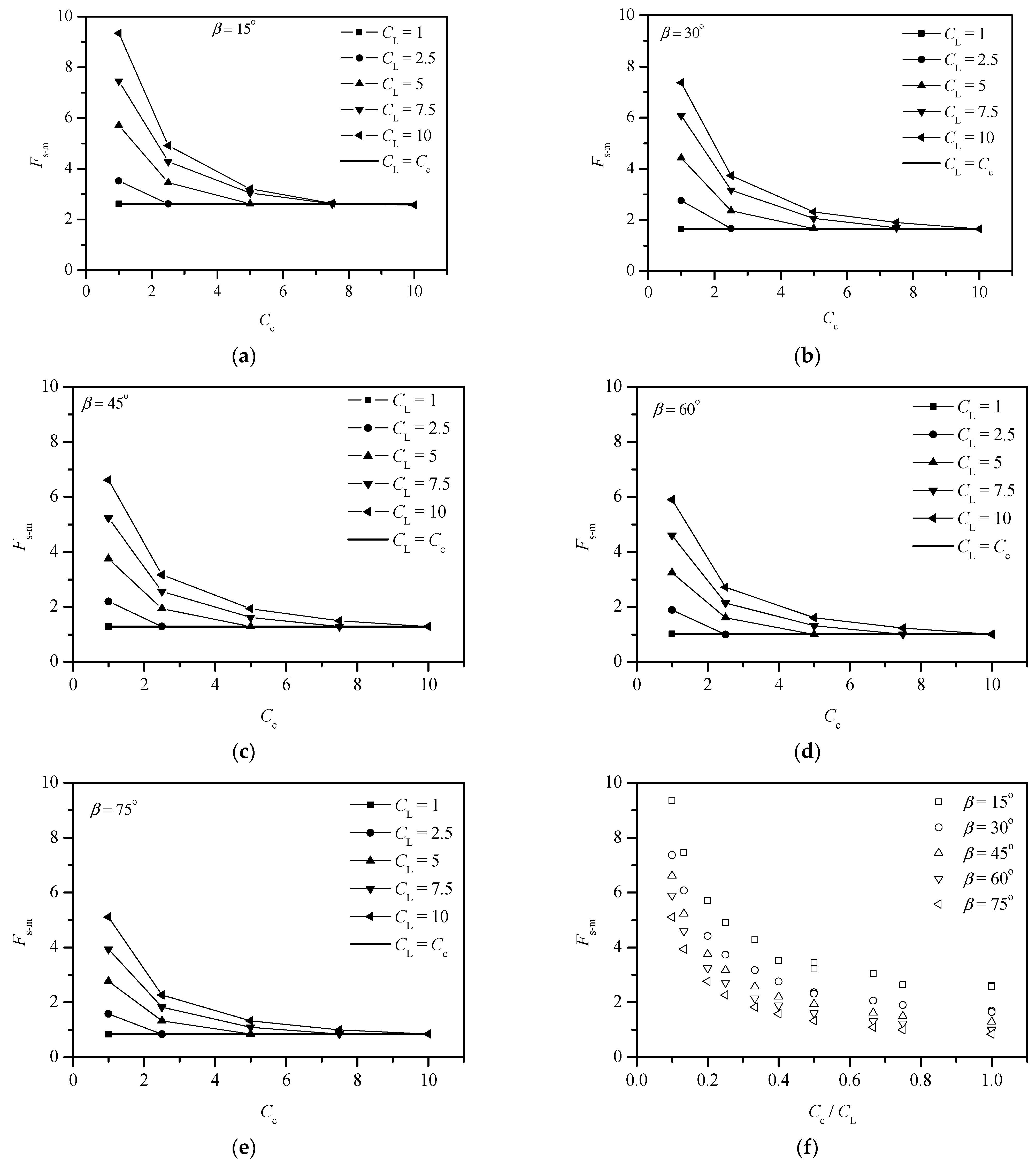
4.2.3. Effect of Model Scale with Varying Angle of Slope

To examine the effect of the reduction coefficients, C_L and C_c, on the reduced-scale model test for different slope angles, five angles of slope are chosen for this parametric analysis (Group VI, Table 2). The finite element (FE) results for various angle slopes (β = 15°, 30°, 45°, 60°, and 75°), with constant values of H_p = 10 m, c_p = 20 kPa, and φ = 20°, are presented in Figure 8. By comparing Figure 4b and Figure 8a,b for the cases with β = 30°, 45°, and 60°, respectively, it is observed that the soil flow patterns at collapse for the reduced model slopes with different slope angles change significantly. While the angle of slope is relatively small (β = 30°), the upper portion of the sliding surface stays almost parallel to the slope surface. In contrast, while the angle of slope is relatively large (β = 60°), the soil flow takes on a wedge-shaped form. From Figure 8, it is evident that as the slope steepens, the volume of soil failure decreases, leading to a lower safety factor.

Figure 9a,e illustrate the impact of the reduction conversion coefficient on the safety factor of the model slope with varying slope angles. The patterns of the F_s-m curves with respect to C_c, C_L, and C_c/C_L closely resemble those observed in the previous studies on cohesion and internal friction angles (see Figure 5 and Figure 7).

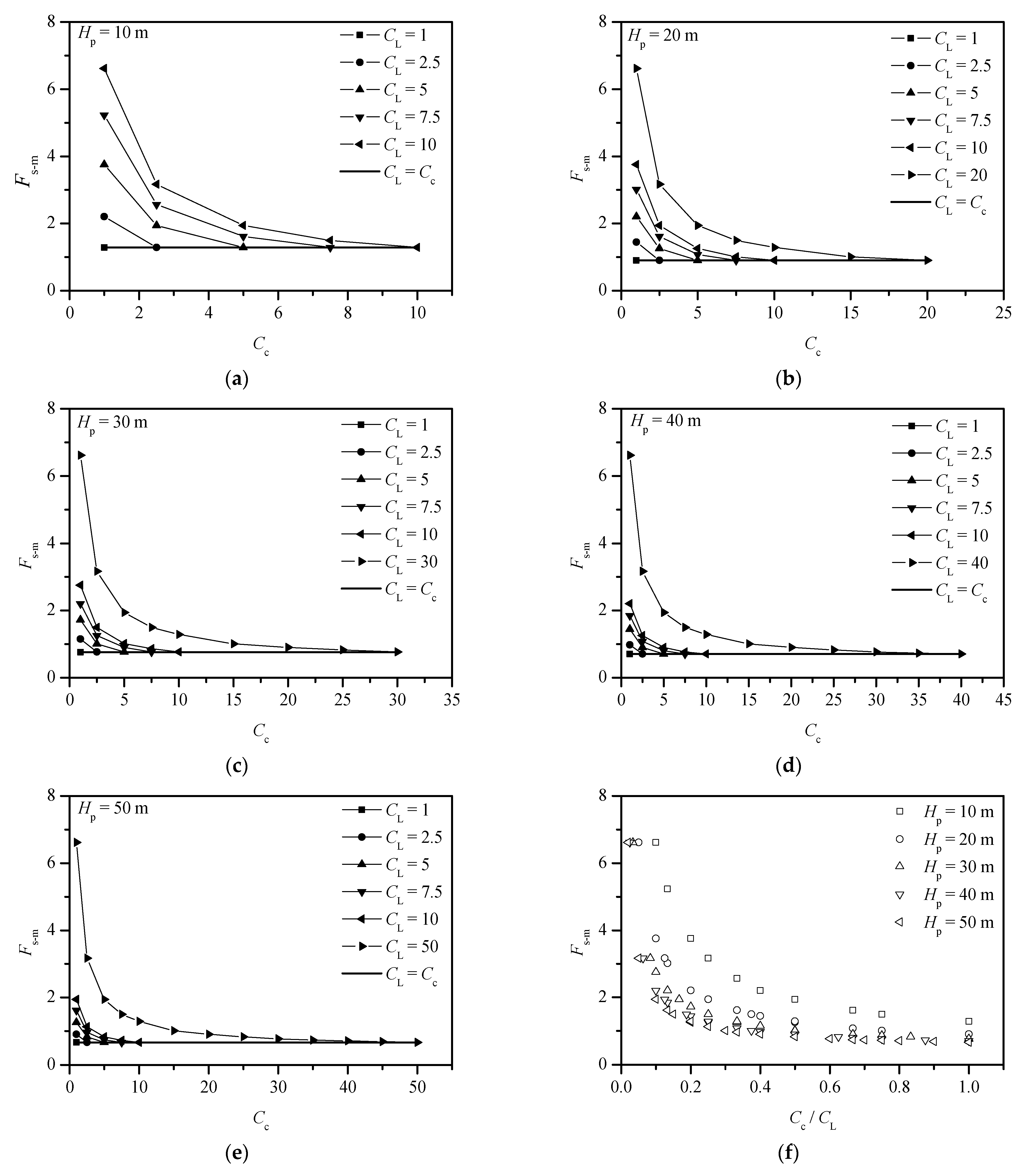
4.2.4. Effect of Model Scale with Varying Slope Height

Five slope heights (H_p = 10, 20, 30, 40, and 50 m) are selected (Group VII, Table 2) to examine the effects of reduced scale of slope stability. The FE results of five slope heights, with constant parameters of c_p = 20 kPa, φ = 20°, and β = 45° are shown in Figure 10. It can be observed that, by comparing Figure 4b and Figure 10a,b for slope heights of H_p = 10 m, 30 m, and 50 m, respectively, at the state of the same C_L and C_c, the sliding surface of the model slope moves upward inwardly with the slope height of the prototype increasing. For one height of a prototype slope, the soil failure zone shrinks to the slope shoulder with increasing C_c and constant C_L (i.e., with increasing C_c/C_L).

Figure 11 plots F_s-m against C_c and C_c/C_L. Similar to the observations from the previous sections, it is seen that, for all slope heights studied, F_s-m decreases with increasing C_c/C_L. The safety factor of the prototype slope is reached when C_c/C_L = 1.0. However, with an increasing ratio of C_c/C_L, the rate of decline in F_s-m is similar to that in Figure 5f (i.e., cohesion effect) and higher than those in Figure 7f and Figure 9f (i.e., internal friction and slope angle effects).

4.3. Failure Mechanism of Slope

From the above discussion, it is clear that the four parameters of a slope (c, φ, β, and H) have a significant impact on slope stability, including both the model slope and the prototype slope. To establish the connection between the behavior of the 1-g model tests and the prototype slopes, the failure mechanisms of the slope will be addressed in the following subsections.

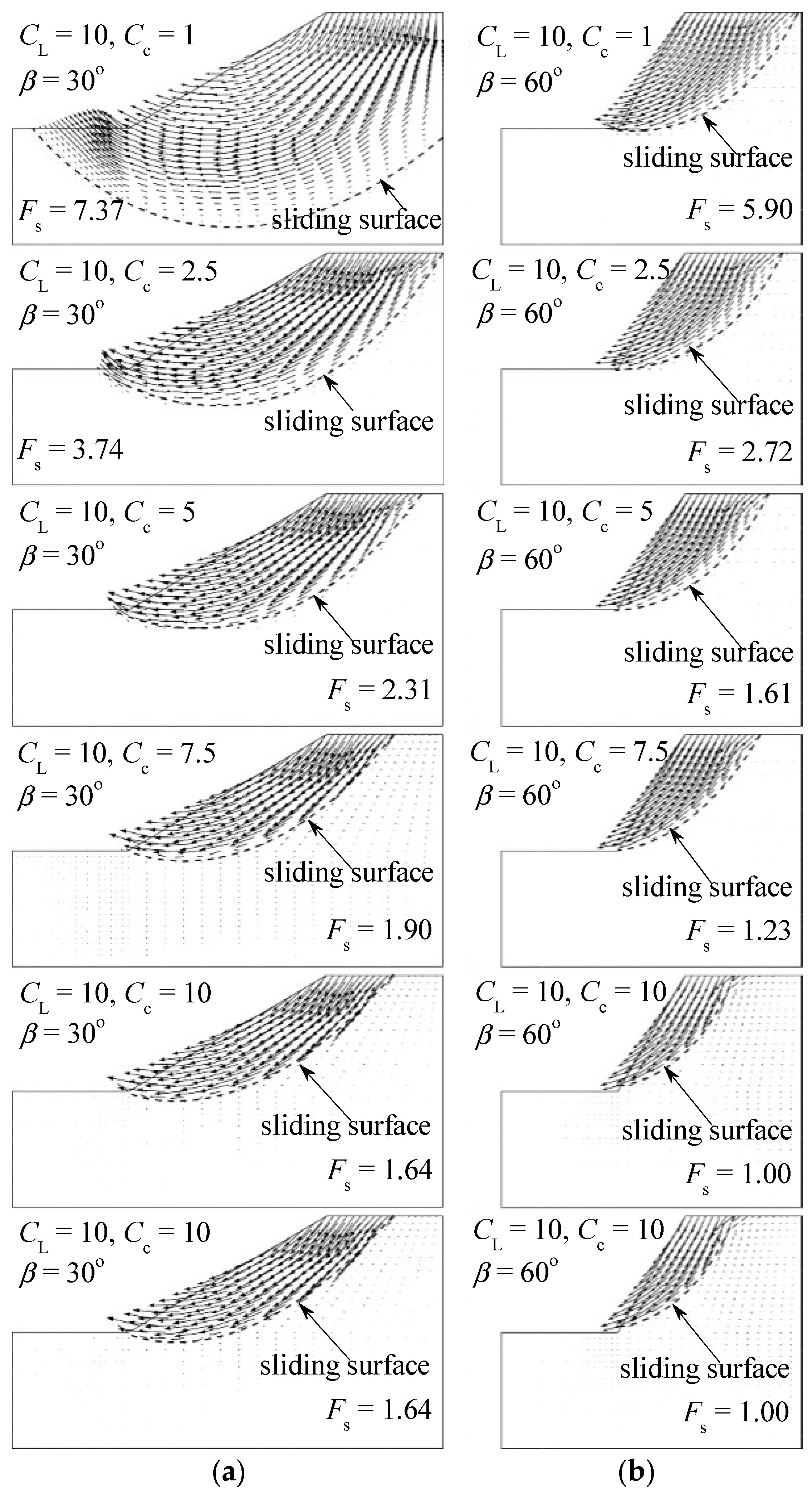
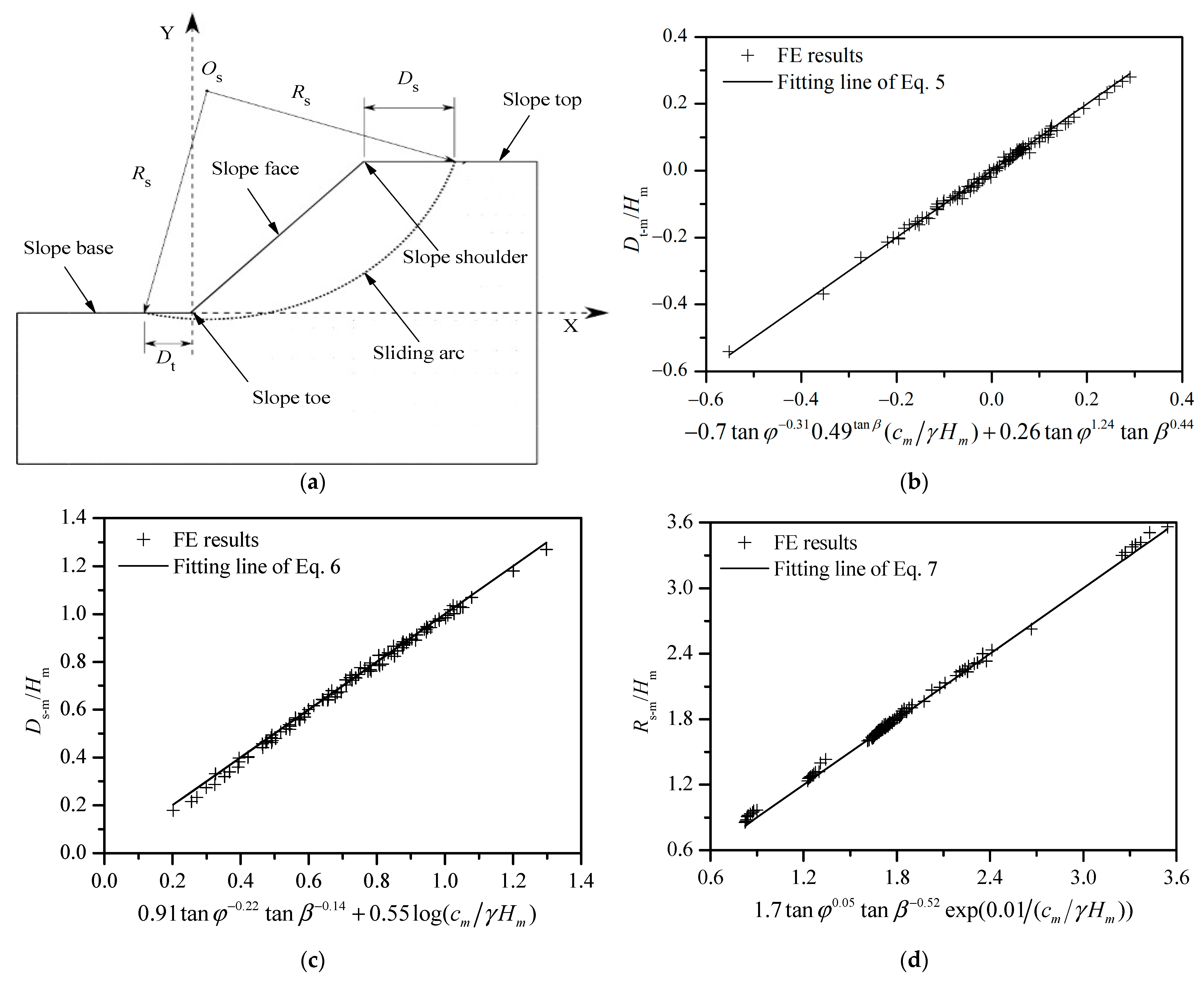
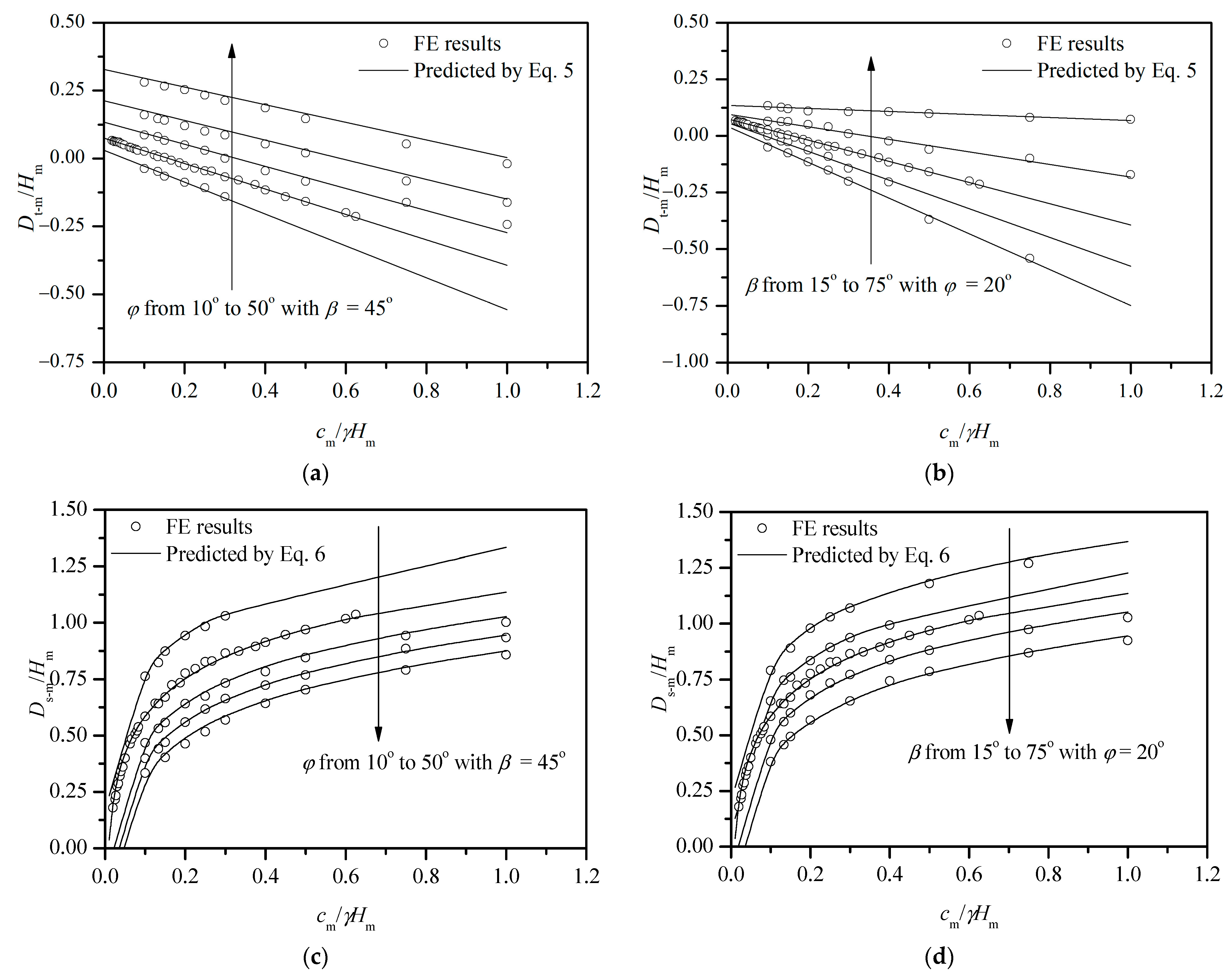
4.3.1. Position of the Slope’s Failure Surface

Among the various methods used for slope stability analysis, the sliding arc approach by Bishop (1955) [2] is chosen for its simplicity and effectiveness. Figure 12a illustrates the sliding arc, with its center denoted by O_s and its radius represented by R_s, within a local coordinate system that is defined with the slope toe as the origin. The sliding arc is characterized by three parameters: R_s, D_s, and D_t. These three parameters represent the radius of the arc, the distance from the arc at the slope top to the slope shoulder, and the distance from the arc at the slope base to the slope toe. For most cases, R_s and D_s are greater than zero, meaning the sliding arc passes through the slope toe. Conversely, D_t < 0 indicates that the sliding arc intersects the slope surface. For the model test, these three parameters can be expressed as D_s-m, D_t-m, and R_s-m.

Based on the results of the numerical simulation parameter analysis, displayed in Figure 4, Figure 5, Figure 6, Figure 7, Figure 8, Figure 9, Figure 10 and Figure 11, the position of the sliding surface can be described using three dimensionless parameters. (i.e., D_s-m/H_m, D_t-m/H_m, and R_s-m/H_m). The three-parameter calculation formulas can be derived through regression analysis (refer to Figure 12b,d, where R² = 0.99 for all fitted lines) and are presented in Equation (5)–(7),

$${\displaystyle \frac{D_{t-m}}{H_m}}=-0.7\tan {\phi }^{-0.31}{0.49}^{\tan \beta }{\displaystyle \frac{c_m}{\gamma H_m}}+0.26\tan {\phi }^{1.24}\tan {\beta }^{0.44}$$

(5)

$${\displaystyle \frac{D_{s-m}}{H_m}}=0.91\tan {\phi }^{-0.22}\tan {\beta }^{-0.14}+0.55\log {\displaystyle \frac{c_m}{\gamma H_m}}$$

(6)

$${\displaystyle \frac{R_{s-m}}{H_m}}=1.7\tan {\phi }^{0.05}\tan {\beta }^{-0.52}\exp ({\displaystyle \frac{0.01}{c_m/\gamma H_m}})$$

(7)

Based on these design formulas, Figure 13 depicts a few design charts for D_t-m/H_m, D_s-m/H_m, and R_s-m/H_m at a given slope. In Figure 13a,b, D_t-m/H_m can be positive and negative. The negative D_t-m/H_m means the sliding arc is passing the slope face. Thus, it is clear that D_t-m/H_m is decreasing to negative (or shrinking to the slope top) with increasing c_m/γH_m and decreasing φ and β. In Figure 13c,d, the width of the slope failure zone at the slope top, D_s-m/H_m, is increasing with increasing c_m/γH_m and decreasing φ and β. The increase in D_s-m/H_m means an increase in slope failure volume. In Figure 13e,f, the sliding arc radius, R_s-m/H_m, decreases with increasing c_m/γH_m and φ and decreasing β. It is clear that the property of soil chosen in the model test (c_m/γH_m) has a significant effect on the failure mechanism of the slope, together with φ and β to a lesser extent.

The effects of slope c_m and φ on the sliding surface were also reported by Cheng et al. (2007) [38]. A similar conclusion was obtained that the sliding surface extends with an increase of c_m and a decrease of φ, which can be observed in Figure 13c of this study. The influence of φ and β on the slope sliding surface was examined by Gao et al. (2013) [39]. They found that as φ and β increase, the changes in the shape of the sliding surface are consistent with the results presented in Figure 13a,d of this study. However, this study has conducted a more comprehensive study covering all slope parameters simultaneously.

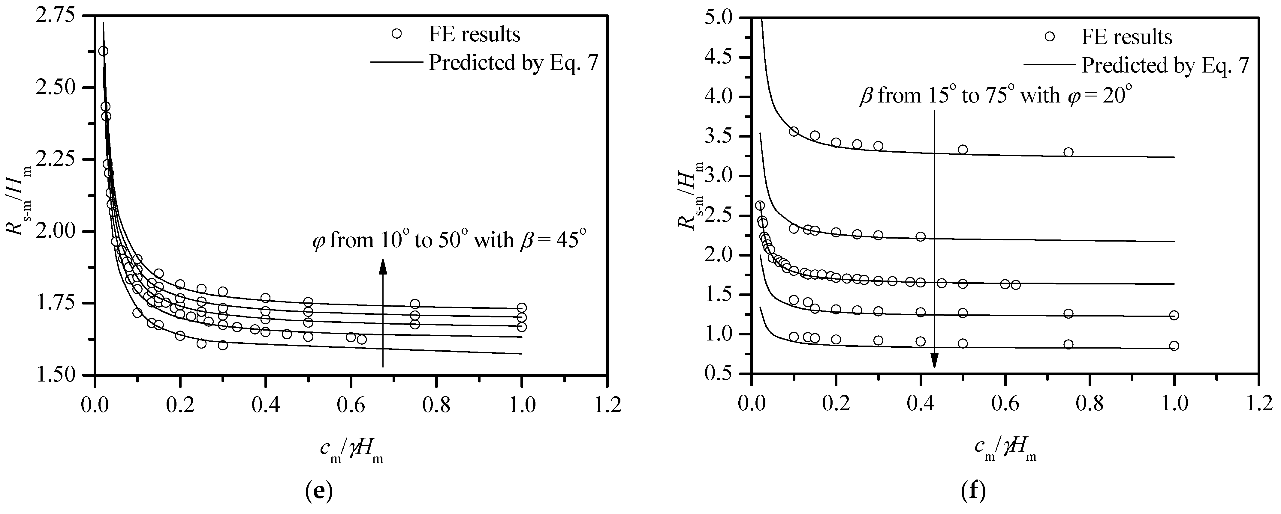
4.3.2. Prediction of the Slope Safety Factor in Model Testing

To predict the safety factor for a 1-g model test and establish a relationship with the safety factor of the corresponding prototype slope, the safety factors obtained from the 1-g model tests were fitted to the slope parameters using the current finite element (FE) analysis, as illustrated in Figure 14a (with an R² value of 0.98). The equation representing the best-fit curve is provided in Equation (8) below.

$$F_{s-m}=5.4\times {1.2}^{\tan \phi }\tan {\beta }^{-0.18}{\displaystyle \frac{c_m}{\gamma H_m}}+0.45\times 3^{\tan \phi }\tan {\beta }^{-0.7}$$

(8)

Based on Equation (8), the effects of c_m/γH_m, φ, and β on the predicted safety factor are shown in Figure 14b,c graphically. It can be seen that F_s-m increases with increasing φ and decreasing β (hence decreasing H_m). Dawson et al. (1999) [3] reported that the slope angle (or slope height) has the opposite effect on the safety factor relative to the cohesion and internal friction angle of soil, which is the same as the phenomenon observed from this study.

4.3.3. Predicting Prototype Slope Behavior

Based on the discussion above, it can be concluded that the stability of a model slope is identical to that of the corresponding prototype when the similarity principle (C_L = C_c) is strictly adhered to. However, in most cases, it is impractical to reach the similarity principle in a 1-g model test; hence, C_L > C_c (non-conformity) is normally encountered for slope tests. Under this condition, the behavior of slopes in a 1-g model test is significantly different from that in the prototype. Thus, this study endeavored to provide an interpolation framework to transform the result from a 1-g model test to the corresponding prototype for the slope sliding surface and slope safety factor.

Based on a 1-g model test results (i.e., D_s-m/H_m, D_t-m/H_m, R_s-m/H_m, and F_s-m), the slope failure surface (i.e., D_s-p/H_p, D_t-p/H_p, and R_s-p/H_p) and the slope safety factor (i.e., F_s-p) for the corresponding prototype slope can be established based on the current numerical results. The best-fitted curves are displayed in Figure 15 (with R² = 0.95~0.98), and the corresponding design formulas are listed in Equations (9)–(12):

$${\displaystyle \frac{D_{t-p}}{H_p}}={\displaystyle \frac{D_{t-m}{C}_c}{H_m{C}_L}}+0.26\tan {\phi }^{1.24}\tan {\beta }^{0.44}(1-{\displaystyle \frac{C_c}{C_L}})$$

(9)

$${\displaystyle \frac{D_{s-p}}{H_p}}={\displaystyle \frac{D_{s-m}}{H_m}}-0.55\log {\displaystyle \frac{C_L}{C_c}}$$

(10)

$${\displaystyle \frac{R_{s-p}}{H_p}}={(1.7\tan {\phi }^{0.05}\tan {\beta }^{-0.52})}^{(1-{\displaystyle \frac{C_L}{C_c}})}{({\displaystyle \frac{R_{s-m}}{H_m}})}^{{\displaystyle \frac{C_L}{C_c}}}$$

(11)

$$F_{s-p}=F_{s-m}{\displaystyle \frac{C_c}{C_L}}+0.45\times 3^{\tan \phi }\tan {\beta }^{-0.7}(1-{\displaystyle \frac{C_c}{C_L}})$$

(12)

These formulae form the foundation for developing a framework to translate the behavior of a uniform slope from a 1-g model test to the prototype.

4.4. Validation of Proposed Interpretation Procedure

Figure 16 presents a flowchart outlining the new framework for interpreting the transition from 1 g model tests to prototype behavior. The proposed interpolation framework is validated against the upper bound solution of limit analysis for the stability of a homogeneous embankment derived by Chen (1975) [37] and the results of finite difference by strength reduction for a homogeneous slope reported by Dawson et al. (1999) [3], with good agreements obtained as shown in Figure 17a,b. The comparisons in terms of sliding surface have been carried out against previously published data [3,4], which is shown in Figure 17c,d. It is evident that the sliding surfaces align closely with each other.

5. Conclusions

This study presents a numerical investigation into the feasibility of using 1-g small-scale model tests for prototype slope design. The study examines both the safety factors and the failure mechanisms of homogeneous clay slopes under self-weight, without external loads, such as rainfall or earthquakes. The shear strength reduction finite element method was employed to simulate the safety factors and failure mechanisms for both the reduced-scale model slopes and the prototype slopes. In the numerical simulation, different scaled model ratios and various soil parameters are considered. Before conducting the parameter analysis, the developed finite element model was first validated against previously published results. The findings show that significant differences exist between the model and prototype slopes in terms of the sliding surface and safety factor for the scaled model tests without conforming to the similarity principle. Based on this comprehensive parametric study, a framework has been developed for applying 1-g small-scale test results to prototype slope design: (i) when all similarity principles are adhered to, the model test results can be directly applied to predict the stability of prototype slopes; (ii) when the small-scale model tests do not fully adhere to the principles of similarity, the developed framework can be used to convert the factor of safety and sliding surface from the model test to those of the prototype slope. This study contributes to the use of scaled physical model tests, which may not fully adhere to the principles of similarity, for evaluating the stability of prototype slopes.

References

1. Peng, B.C.; Zhang, L.; Xu, Z.Y.; Cui, P.L.; Liu, Y.Y. Numerical Stability Analysis of Sloped Geosynthetic Encased Stone Column Composite Foundation under Embankment Based on Equivalent Method. Buildings 2024, 14, 2681. [Google Scholar] [CrossRef]
2. Bishop, A.W. The use of the slip circle in the stability analysis of slopes. Geotechnique 1955, 5, 7–17. [Google Scholar] [CrossRef]
3. Dawson, E.M.; Roth, W.H.; Drescher, A. Slope stability analysis by strength reduction. Géotechnique 1999, 49, 835–840. [Google Scholar] [CrossRef]
4. Griffiths, D.V.; Lane, P.A. Slope stability analysis by finite elements. Geotechnique 1999, 49, 653–654. [Google Scholar] [CrossRef]
5. Hosseini, S.; Astaraki, F.; Imam, S.M.R.; Chalabii, J.; Movahedi Rad, M. Investigation of Shear Strength Reduction Method in Slope Stability of Reinforced Slopes by Anchor and Nail. Buildings 2024, 14, 432. [Google Scholar] [CrossRef]
6. Song, S.; Feng, X.; Rao, H.; Zheng, H. Treatment design of geological defects in dam foundation of Jinping I hydropower station. J. Rock Mech. Geotech. Eng. 2013, 5, 342–349. [Google Scholar] [CrossRef]
7. Chen, Y.; Zhang, L.; Yang, B.; Dong, J.; Chen, J. Geomechanical model test on dam stability and application to Jinping High arch dam. Int. J. Rock Mech. Min. Sci. 2015, 76, 1–9. [Google Scholar] [CrossRef]
8. Liu, H.; Zhou, M.; Hu, Y.; Hossain, M.S. Behaviour of ball penetrometer in uniform single- and double-layer clays. Geotechnique 2013, 63, 682–694. [Google Scholar]
9. Sloan, S.W. Geotechnical stability analysis. Géotechnique 2013, 63, 531–571. [Google Scholar] [CrossRef]
10. Lu, P.; Wu, H.; Qiao, G.; Li, W.; Scaioni, M.; Feng, T.; Liu, S.; Chen, W.; Li, N.; Liu, C.; et al. Model test study on monitoring dynamic process of slope failure through spatial sensor network. Environ. Earth Sci. 2015, 74, 3315–3332. [Google Scholar] [CrossRef]
11. Lin, P.; Liu, X.; Zhou, W.; Wang, R.; Wang, S. Cracking, stability and slope reinforcement analysis relating to the Jinping dam based on a geomechanical model test. Arab. J. Geosci. 2015, 8, 4393–4410. [Google Scholar]
12. Ling, H.I.; Wu, M.; Leshchinsky, D.; Leshchinsky, B. Centrifuge modeling of slope instability. J. Geotech. Geoenviron. Eng. 2009, 135, 758–767. [Google Scholar]
13. Ng, C.; Kamchoom, V.; Leung, A.K. Centrifuge modelling of the effects of root geometry on transpiration-induced suction and stability of vegetated slopes. Landslides 2016, 13, 925–938. [Google Scholar] [CrossRef]
14. Schofield, A.N. Use of centrifugal model testing to assess slope stability. Can. Geotech. J. 1978, 15, 14–31. [Google Scholar]
15. Yang, K.; Zhu, Y.; Guo, H.; Xie, Y.; Wang, Z. Centrifugal Model Test of Multi-Level Slope under Combined Support of Pile-Anchor and Frame-Anchor. Buildings 2024, 14, 2680. [Google Scholar] [CrossRef]
16. Weng, M.; Chen, T.; Tsai, S. Modeling scale effects on consequent slope deformation by centrifuge model tests and the discrete elementmethod. Landslides 2017, 14, 981–993. [Google Scholar]
17. Fumagalli, E. Statical and Geomechanical Models, 1st ed.; Springer: Vienna, Austria, 1973; pp. 1–32. [Google Scholar]
18. Mcnearny, R.L.; Abel Jr, J.F. Large-scale two-dimensional block caving model tests. Int. J. Rock Mech. Min. Sci. Geomech. Abstr. 1993, 30, 93–109. [Google Scholar] [CrossRef]
19. Luo, X.; Liu, D.; Wu, J.; Cheng, S.; Shen, H.; Xu, K.; Huang, X. Model test study on landslide under rainfall and reservoir water fluctuation. Yanshilixue Yu Gongcheng Xuebao 2005, 24, 2476–2483. [Google Scholar]
20. Fan, Z.; Kulatilake, P.; Peng, J.; Che, W.; Li, Y.; Meng, Z. In-flight excavation of a loess slope in a centrifuge model test. Geotech. Geol. Eng. 2016, 34, 1577–1591. [Google Scholar]
21. Wang, K.; Lin, M. Initiation and displacement of landslide induced by earthquake—A study of shaking table model slope test. Eng. Geol. 2011, 122, 106–114. [Google Scholar]
22. Kumsar, H.; Aydan, Ö.; Ulusay, R. Dynamic and Static Stability Assessment of Rock Slopes Against Wedge Failures. Rock Mech. Rock Eng. 2000, 33, 31–51. [Google Scholar]
23. Jia, G.W.; Zhan, T.L.T.; Chen, Y.M.; Fredlund, D.G. Performance of a large-scale slope model subjected to rising and lowering water levels. Eng. Geol. 2009, 106, 92–103. [Google Scholar]
24. Moriwaki, H.; Inokuchi, T.; Hattanji, T.; Sassa, K.; Ochiai, H.; Wang, G. Failure processes in a full-scale landslide experiment using a rainfall simulator. Landslides 2004, 1, 277–288. [Google Scholar]
25. Saghaee, G.; Mousa, A.A.; Meguid, M.A. Plausible failure mechanisms of wildlife-damaged earth levees: Insights from centrifuge modeling and numerical analysis. Can. Geotech. J. 2017, 54, 1496–1508. [Google Scholar]
26. Yang, K.H.; Zornberg, J.G.; Liu, C.N.; Lin, H.D. Stress distribution and development within geosynthetic-reinforced soil slopes. Geosynth. Int. 2012, 19, 62–78. [Google Scholar]
27. Zhou, B.; Zhong, H.; Yang, K.; Yang, X.; Cai, C.; Xiao, J.; Liu, Y.; Yuan, B. A Study on the Factors Influencing High Backfill Slope Reinforced with Anti-Slide Piles under Static Load Based on Numerical Simulation. Buildings 2024, 14, 799. [Google Scholar] [CrossRef]
28. Leung, A.K.; Kamchoom, V.; Ng, C. Influences of root-induced soil suction and root geometry on slope stability: A centrifuge study. Can. Geotech. J. 2016, 54, 291–303. [Google Scholar]
29. Smith, I.M.; Hobbs, R. Finite element analysis of centrifuged and built-up slopes. Geotechnique 1974, 24, 531–559. [Google Scholar] [CrossRef]
30. Simulia, D.C.S. Abaqus 6.11 Analysis User’s Manual; Dassault Systemes, Providence: Johnston, RI, USA, 2011. [Google Scholar]
31. Zheng, H.; Tham, L.G.; Liu, D. On two definitions of the factor of safety commonly used in the finite element slope stability analysis. Comput. Geotech. 2006, 33, 188–195. [Google Scholar]
32. Chen, X.; Wu, Y.; Yu, Y.; Liu, J.; Xu, X.F.; Ren, J. A two-grid search scheme for large-scale 3-D finite element analyses of slope stability. Comput. Geotech. 2014, 62, 203–215. [Google Scholar]
33. Matsui, T.; San, K. Finite Element Slope Stability Analysis by Shear Strength Reduction Technique. Soils Found. 2008, 32, 59–70. [Google Scholar] [CrossRef]
34. Ugai, K. A method of calculation of total safety factor of slope by elasto-plastic FEM. Soils Found. 2008, 29, 190–195. [Google Scholar] [CrossRef] [PubMed]
35. Zhou, M.; Hossain, M.S.; Hu, Y.; Liu, H. Scale Issues and Interpretation of Ball Penetration in Stratified Deposits in Centrifuge Testing. J. Geotech. Geoenviron. Eng. 2016, 142, 04015103. [Google Scholar] [CrossRef]
36. Duncan, J.M. State of the Art: Limit Equilibrium and Finite-Element Analysis of Slopes. J. Geotech. Eng. 1996, 123, 577–596. [Google Scholar] [CrossRef]
37. Chen, W.-F. Limit Analysis and Soil Plasticity; Elsevier Scientific Pub. Co.: Amsterdam, The Netherlands, 1975. [Google Scholar]
38. Cheng, Y.M.; Lansivaara, T.; Wei, W.B. Two-dimensional slope stability analysis by limit equilibrium and strength reduction methods. Comput. Geotech. 2007, 34, 137–150. [Google Scholar] [CrossRef]
39. Gao, Y.F.; Zhang, F.; Lei, G.H.; Li, D.Y. An extended limit analysis of three-dimensional slope stability. Géotechnique 2013, 63, 518–524. [Google Scholar] [CrossRef]
Figure 1. Numerical model of reduced-scale model test of homogeneous slope: (a) schematic diagram of reduced scale model; (b) mesh of FE model.
Buildings 15 01015 g001
Figure 2. Validation: (a) validation of this study against finite difference by Dawson et al. (1999) [3]; (b) validation of this study against finite difference by Griffiths and Lane (1999) [4].
Buildings 15 01015 g002
Figure 3. Effect of cp, φ, β, and Hp on slope stability for prototype slope: (a) various cp with φ = 20°, β = 45°, Hp = 10 m; (b) various φ with cp = 20 kPa, β = 45°, Hp = 10 m; (c) various β with φ = 20°, cp = 20 kPa, Hp = 10 m; (d) various Hp with φ = 20°, cp = 20 kPa, β = 45°.
Buildings 15 01015 g003
Figure 4. Effect of the reduction coefficients on soil flow mechanism of reduced scale model slope by varying cp with φ = 20°, β = 45°, and Hp = 10 m: (a) cp = 10 kPa; (b) cp = 20 kPa.
Buildings 15 01015 g004
Figure 5. Effect of the reduction coefficients on the safety factor for the reduced scale model slope by varying cp with φ = 20°, β = 45°, and Hp = 10 m: (a) cp = 10 kPa; (b) cp = 20 kPa; (c) cp = 30 kPa; (d) cp = 40 kPa; (e) cp = 50 kPa; (f) Fs-m versus Cc/CL with various cp.
Buildings 15 01015 g005
Figure 6. Effect of the reduction coefficients on the soil flow mechanism of the reduced-scale model slope by varying φ with cp = 20 kPa, β = 45°, and Hp = 10 m: (a) φ = 10°; (b) φ = 40°.
Buildings 15 01015 g006
Figure 7. Effect of the reduction coefficients on the safety factor for the reduced-scale model slope by varying φ with cp = 20 kPa, β = 45°, and Hp = 10 m: (a) φ = 10°; (b) φ = 20°; (c) φ = 30°; (d) φ = 40°; (e) φ = 50°; (f) Fs-m versus Cc/CL with various φ.
Buildings 15 01015 g007
Figure 8. Effect of the reduction coefficients on the soil flow mechanism of the reduced-scale model slope by varying β with cp = 20 kPa, φ = 20° and Hp = 10 m: (a) β = 30°; (b) β = 60°.
Buildings 15 01015 g008
Figure 9. Effect of the reduction coefficients on safety factor for reduced-scale model slope by varying β with cp = 20 kPa, φ = 20°, and Hp = 10 m: (a) β = 15°; (b) β = 30°; (c) β = 45°; (d) β = 60°; (e) β = 75°; (f) Fs-m versus Cc/CL with various β.
Buildings 15 01015 g009
Figure 10. Effect of the reduction coefficients on the soil flow mechanism of the reduced-scale model slope by varying Hp with cp = 20 kPa, φ = 20°, and β = 45°: (a) Hp = 30 m; (b) Hp = 50 m.
Buildings 15 01015 g010
Figure 11. Effect of the reduction conversion coefficients on safety factor for the reduced-scale model slope by varying Hp with cp = 20 kPa, φ = 20°, and β = 45°: (a) Hp = 10 m; (b) Hp = 20 m; (c) Hp = 30 m; (d) Hp = 40 m; (e) Hp = 50 m; (f) Fs-m versus Cc/CL with various Hp.
Buildings 15 01015 g011
Figure 12. Location of the sliding arc of reduced-scale model test and data fittings: (a) local coordinate system; (b) data fitting for Dt-m; (c) data fitting for Ds-m; (d) data fitting for Rs-m.
Buildings 15 01015 g012
Figure 13. Design charts for the sliding arc of the reduced-scale model slope: (a) predicted Dt-m versus cm/γHm with various φ and β = 45°; (b) predicted Dt-m versus cm/γHm with various β and φ = 20°; (c) predicted Ds-m versus cm/γHm with various φ and β = 45°; (d) predicted Ds-m versus cm/γHm with various β and φ = 20°; (e) predicted Rs-m versus cm/γHm with various φ and β = 45°; (f) predicted Rs-m versus cm/γHm with various β and φ = 20°.
Buildings 15 01015 g013aBuildings 15 01015 g013b
Figure 14. Design charts for the safety factor of the reduced-scale model slope: (a) data fitting for Fs-m; (b) predicted Fs-m versus cm/γHm with various φ and β = 45°; (c) predicted Fs-m versus cm/γHm with various β and φ = 20°.
Buildings 15 01015 g014
Figure 15. Data fittings for sliding arc and safety factor of prototype slope: (a) data fitting for Dt-p; (b) data fitting for Ds-p; (c) data fitting for Rt-p; (d) data fitting for Fs-p.
Buildings 15 01015 g015
Figure 16. Procedure for prediction of slope stability from a reduced-scale model test.
Buildings 15 01015 g016
Figure 17. Validation of prediction using the proposed approach: (a) validation of the prediction for safety factor with β = 60°; (b) validation of the prediction for safety factor with β = 75°; (c) validation of the prediction for sliding surface with β = 26.57°; (d) validation of the prediction for sliding surface with β = 45°.
Buildings 15 01015 g017