Article

Development of an Optimal Machine Learning Model to Predict CO2 Emissions at the Building Demolition Stage

1
Academic-Research Digital Convergence Scale-Up Platform Center, Kyungpook National University, Daegu 41566, Republic of Korea
2
Department of Undeclared Majors, Kyungpook National University, Daegu 41566, Republic of Korea
*
Author to whom correspondence should be addressed.
Buildings 2025, 15(4), 526; https://doi.org/10.3390/buildings15040526
Submission received: 18 December 2024 / Revised: 29 January 2025 / Accepted: 5 February 2025 / Published: 9 February 2025
(This article belongs to the Section Building Energy, Physics, Environment, and Systems)

Abstract

:
The construction industry accounts for approximately 28% of global CO2 emissions, and emission management at the building demolition stage is important for achieving carbon neutrality goals. Systematic studies on the demolition stage, however, are still lacking. In this study, research on the development of optimal machine learning (ML) models was conducted to predict CO2 emissions at the demolition stage. CO2 emissions were predicted by applying various ML algorithms (e.g., gradient boosting machine [GBM], decision tree, and random forest), based on the information on building features and the equipment used for demolition, as well as energy consumption data. GBM was selected as a model with optimal prediction performance. It exhibited very high accuracy with R2 values of 0.997, 0.983, and 0.984 for the training, test, and validation sets, respectively. The GBM model also showed excellent results in generalization performance, and it effectively learned the data patterns without overfitting in residual analysis and mean absolute error (MAE) evaluation. It was also found that features such as the floor area, equipment, wall type, and structure significantly affect CO2 emissions at the building demolition stage and that equipment and the floor area are key factors. The model developed in this study can be used to support decision-making at the initial design stage, evaluate sustainability, and establish carbon reduction strategies. It enables efficient data collection and processing and provides scalability for various analytical approaches compared to the existing life cycle assessment (LCA) approach. In the future, it is deemed necessary to develop ML tools that enable comprehensive assessment of the building life cycle through system boundary expansion.

1. Introduction

Due to the sharp increase in greenhouse gas (GHG) emissions, global warming has become one of the most serious environmental issues. The average temperature of the Earth increased by 0.85 degrees from the late 19th century to 2012 due to the greenhouse effect [1], and it is still increasing at a rate of 2 ppm annually [2,3]. Therefore, the world has promoted carbon emission reduction policies to control GHG concentrations and slow down climate change, calling for actions to achieve carbon neutrality by 2050 through the Paris Agreement.
Construction-related industries consume approximately one-third of the world’s total energy and account for approximately 28% of global CO2 emissions [4]. In most countries, the construction industry is responsible for increasing carbon emissions [5,6], and it is essentially required to reduce carbon emissions over the life cycle of buildings. Furthermore, 11% of CO2 emissions from the construction sector result from the production of building materials, and reducing CO2 emissions in this process is considered an effective method [7]. To this end, efforts have been made to reduce CO2 emissions from the building material production process through the recycling of construction and demolition waste (CDW). As such, construction-related industries and researchers have made efforts and conducted research to reduce the environmental effects of CDW through waste management and recycling after building demolition. For example, Ivanica et al. (2022) developed a life cycle inventory database on the demolition process for five houses in southern Germany and conducted an environmental assessment, including CO2, based on the database [7]. These authors paid attention to the fact that previous studies on LCA did not include the demolition stage by assuming that the impact of the end-of-life (EoL) stage in the life cycle was insignificant and constructed LCI information on the demolition process. Liu et al. (2020) conducted research on the CO2 and cost-reduction effects of recycling demolition waste (DW) in Guangzhou City, China [8]. They showed that the environmental effects and economic costs of the building life cycle can be reduced by recycling DW. Cha et al. (2020) constructed data on CO2 and cost from the generation of waste to its transport and disposal by structure for 1034 residential buildings in Korea [9]. Based on the data, they presented recycling potential results according to the building structure and waste type. They proposed a method to comprehensively consider the environment and cost according to the building structure and waste type at the building EoL stage. Hao and Ma (2023) conducted research on CO2 emissions due to the improvement and reduction in the CDW recycling rate in a building energy retrofit project in China [10]. They showed that improving the recycling rate of inert and combustible waste using system dynamics has a significant effect on CO2 reduction. Peng et al. (2021) conducted research on carbon emission reduction through the recycling of CDW for three port cities in southern China [11]. They predicted carbon saving potential in 2060 through CDW recycling, showing that it is possible to save the same amount of carbon as carbon emissions from raw materials. Zhao et al. (2023) investigated CO2 emissions from the onsite, intermediate, and final disposal and transportation processes of CDW in the city of Kitakyushu, Japan [12]. They showed that the recycling of CDW has a carbon emission reduction effect of approximately 21% compared to the same amount of new materials. These are studies on CO2 emissions and their reduction through CDW management, and they are focused on CO2 emissions and reduction measures according to management methods, such as the transport and recycling of CDW. In particular, for the building EoL stage, studies have been mainly conducted on the management and environmental impacts of DW, including CO2 emissions, flow, and reduction measures according to waste transport and disposal after building demolition [13]. However, there are few studies that are targeted at or include the demolition stage [7,14]. The demolition stage, however, can provide criteria to be considered when buildings are designed and constructed, and it is an important element in determining whether materials can be reused or recycled [7]. This is because CO2 information for the building demolition stage can be used for the calculation of accurate CO2 emissions over the entire building life cycle, environmental performance optimization at the initial design stage, and recycling evaluation. Therefore, current research on CDW management and CO2 evaluation for the building EoL stage needs to be expanded to more in-depth research for the demolition stage.
It is not easy to predict CO2 emissions at the building demolition stage, because accurately predicting CO2 emissions by reflecting the demolition method, building structure and size, and material type for various buildings is difficult for simple calculation methods. In addition, since it requires considerable manpower and time to collect actual field data for calculating CO2 emissions at the building demolition stage, constructing sufficient data is not easy. To address these problems, AI technology has been introduced and successfully applied to various industries, and various studies have also been conducted on technologies for CDW management. For example, Razi and Ansari (2024) tested various machine learning (ML) models and showed optimized results to balance nonlinear relationships among four goals (time, cost, energy consumption, and CO2 emissions) in a construction project [15]. In the study, the artificial neural network (ANN) model showed high performance with a CO2-prediction accuracy of 97.99%. Fang et al. (2021) developed a model using the random forest (RF) algorithm to predict CO2 emissions from the construction stage of a building at the design stage [16]. They used data for 38 buildings, and the performance of the RF model showed an R2 value of approximately 0.64. In addition, a number of researchers [17,18,19,20,21,22,23] developed various ML models to develop tools for predicting and managing the amount of CDW generated. Some researchers conducted studies on CO2 emissions for construction activities using ML models to evaluate CO2 emissions from buildings. As for the building EoL stage, most studies were conducted on the amount of CDW generated, as well as CO2 emissions and reduction measures according to the CDW disposal method (e.g., recycling, reuse, incineration, and landfill) using ML. Previous studies focused mostly on construction activities or CDW processing methods, and few studies systematically predicted CO2 emissions at the building demolition stage. Therefore, it is necessary to develop ML models for accurately predicting CO2 emissions by reflecting the characteristics of the building demolition stage. This should be performed based on data collection and analysis in consideration of various factors at the demolition stage.
Based on the recent research trends, the research gap related to the building EoL stage is a demand for technology that can accurately predict CO2 emissions for the demolition stage. Conventional LCA studies have often overlooked the nonlinear and highly variable factors influencing emissions during the demolition stage of a building’s life cycle. Furthermore, such studies typically rely on static emission factors or averages, failing to adequately account for the impacts of specific factors such as structural types, equipment usage, and demolition methods. In this context, a data-driven approach utilizing ML has the potential to improve the precision of CO2-emission predictions by integrating complex and nonlinear variables of the demolition stage. Moreover, ML-based dynamic modeling, which conventional LCA models cannot provide, can offer precise predictions of CO2 emissions tailored to specific buildings and operational conditions. Therefore, the main purpose of this study is to develop prediction models for CO2 emissions at the demolition stage by reflecting various nonlinear factors of the building (e.g., equipment type used for demolition, building structure, area, usage, and material type) using ML. Specifically, inventory data were collected on building features (e.g., building structure, usage, area, and material types of major structures), the types of equipment used for demolition, and energy consumption for various buildings at the demolition stage. In addition, various ML algorithms were applied to develop an optimal CO2 prediction model for the demolition stage. Models were derived by finding optimal values of hyperparameters (HPs) for each algorithm, and the performance of the models was compared to present a CO2-prediction model with the highest prediction performance. The main content included in this paper to achieve the purpose of this study is as follows:
  • Construction of CO2 inventory raw data at the demolition stage based on the analysis of building features, demolition equipment, and energy consumption for 186 buildings;
  • Data preprocessing and dataset construction to improve the performance of ML models;
  • Development of CO2-prediction models with optimal performance by performing feature engineering and HPs tuning for various ML algorithms;
  • Analysis of factors that affect CO2 emissions at the building demolition stage;
  • Derivation of a CO2-prediction model with the highest prediction performance and an examination of its generalization performance;
  • Proposal of research directions through the comparison of results with previous studies and discussion.

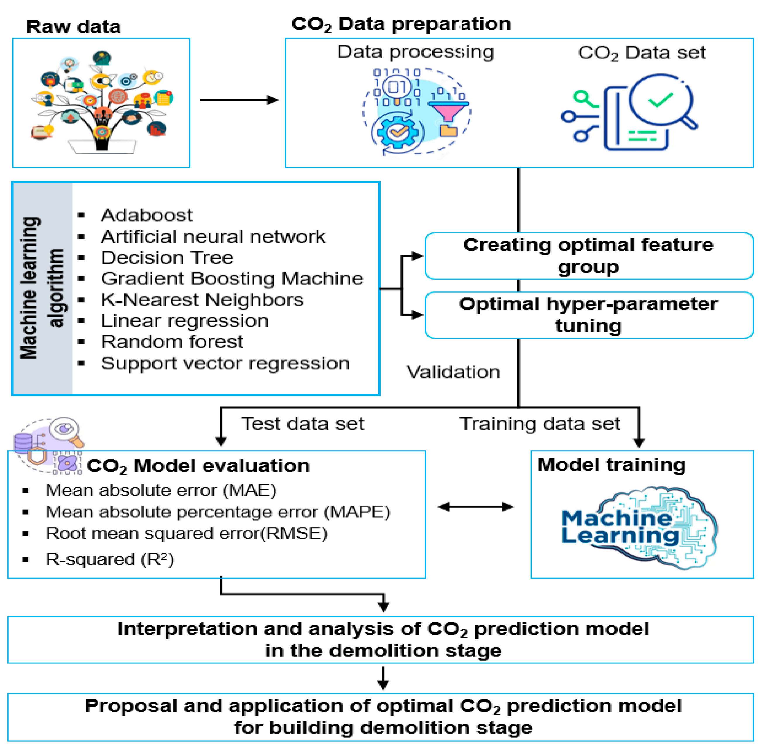
2. Materials and Methods

Figure 1 shows the flowchart of this study to develop a model for predicting CO2 emissions at the building demolition stage, including data collection and processing, types of algorithms used and optimization method, evaluation, and proposal of an optimal model through the interpretation of CO2 models. In the data-collection phase, a dataset was constructed that included building information along with energy consumption and CO2 emission data during the demolition stage. In the data processing phase, data quality improvement tasks were performed through missing value handling, outlier removal, and standardization. Prior to model development using various ML algorithms, correlation analysis was conducted to identify the key variables influencing CO2 emissions, which were prioritized in the model training process. To achieve optimal predictive performance for each ML algorithm, hyperparameter optimization was carried out for each model. The developed models were evaluated for predictive accuracy using performance metrics, and residual analysis was conducted to assess generalization performance and detect potential overfitting. Ultimately, the study proposed the optimal ML model for predicting CO2 emissions during the building demolition stage.

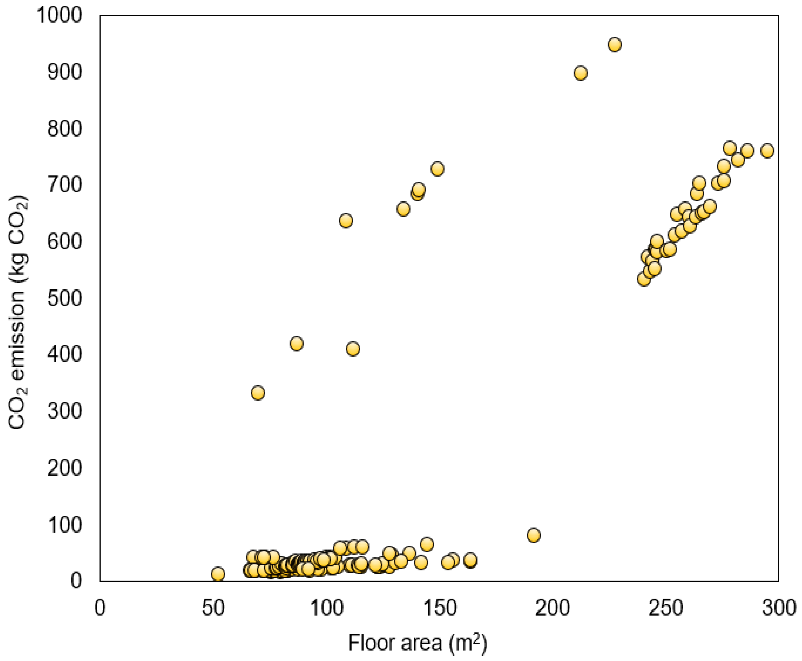
2.1. Data Collection of the Building Demolition Stage

In this study, the building information surveyed in previous studies [24,25] was utilized. The target areas are the demolition sites of redevelopment areas in Daegu (35.88 N latitude, 128.61 E longitude) and Busan (35.87 N latitude, 128.63 E longitude) City, which are metropolitan cities in the southern part of Korea. They include building feature information for 186 buildings (102 for project A and 84 for project B). As for the building feature information, the data were collected by recording the structure, usage, area, wall material, roof material, and number of floors through building ledger records and on-site measurements before demolition. The building survey was conducted using a laser distance meter to measure the floor area and building height, and a digital camera was used to capture images of wall structures and material types. In the case of the demolition process, data on the type, work capability, and energy consumption of the equipment used in each building were secured through inquiries to the companies in charge of the task. Subsequently, interviews were conducted with demolition contractors to gather information on the types of demolition equipment used, working hours, and fuel consumption. The collected data were recorded using a standardized data-collection form. Table 1 shows the parameters, units, and sources of the collected data.

2.2. Calculation of CO2 Emissions at the Demolition Stage

In this study, the types of mechanical equipment used for building demolition were investigated, and it was observed that the combination of equipment varied depending on the building structure. The equipment used for demolition was classified into three types. A-type equipment (crawler excavator [1.0 m3] and hydraulic breaker [1.0 m3]) was used for reinforced concrete structures, B-type equipment (crawler excavator [0.7 m3] and hydraulic breaker [0.7 m3]) for concrete-brick structures, and C-type equipment (crawler excavator [1.0 m3]) for masonry and wooden structures. The main energy source of equipment was diesel, and CO2 emissions were calculated from diesel consumption. Diesel consumption refers to the amount used, depending on the demolition equipment and the demolition area. It is generally measured by the amount of fuel consumed during combustion by the equipment. The fuel consumption required for demolition work can vary based on the type of equipment, working hours, workload intensity, building structure, and demolition method. Since the carbon emission factor of the energy source used is a fixed value, carbon emissions are proportional to fuel consumption. Additionally, the characteristics of the building influence the required equipment and fuel consumption, which in turn impacts CO2 emissions. Therefore, CO2 emissions at the building demolition stage can be calculated from fuel consumption through the CO2 emission factor of the energy source used. CO2 emissions at the demolition stage were calculated using Equation (1):
C O 2 E m i s s i o n d e m o l i t i o n   s t a g e = E i c f i ,
where C O 2 E m i s s i o n d e m o l i t i o n   s t a g e denote CO2 emissions (kg CO2/m2) at the demolition stage, E i is the fuel consumed ( L / m 2 ) by the demolition equipment i, and c f i is the carbon emission coefficient (kg CO2/   L ) of unit fuel used by equipment i.

2.3. Feature Engineering

The use of detailed data preprocessing techniques can increase the prediction and classification accuracy of supervised learning models [26]. Data preprocessing is essential, and it is known that most engineering efforts are made for it [27]. In fact, many of the data generated include outliers or missing values. Therefore, data preprocessing is considered an important step for constructing reliable data [28]. Data standardization is a data preprocessing technique that converts the average of data to 0 and the standard deviation to 1 for scaling variables with different units or sizes on the same basis. This ensures that the influence between variables is fairly reflected in model learning. Therefore, in this study, data standardization (Equation (2)) was performed to construct a reliable dataset and improve the performance of prediction models:
x s t a n d a r d i z a t i o n = x μ σ ,
where x is the element of data, μ is the mean of the data, and σ is the standard deviation of the data.
Table 2 shows the statistics on the fuel consumption and CO2 emissions of the dataset after data preprocessing. Table 2 presents the fuel consumption by equipment used for the demolition of individual buildings and the resulting CO2 emissions calculated based on these data. The fuel consumption per unit area (L/m2) is defined as the total fuel consumption for the demolition work divided by the total floor area of the building. Additionally, the CO2 emissions per unit area (kg CO2/m2) were calculated using the fuel consumption and Equation (1). Energy consumption (L/m2) and CO2 emissions (kg-CO2/m2) have significant differences between the minimum and maximum values. This results from various features of buildings (e.g., building size, structure, and types of materials used) and the equipment used for demolition. The increase in demolition-work volume with the size of a building generally leads to higher fuel consumption and CO2 emissions. However, the differences in fuel consumption and CO2 emissions per unit area are attributed to variations in demolition methods and equipment usage, which are influenced by the building’s structural and material characteristics. In addition, high standard deviation and variance values indicate that CO2 emissions significantly differ from the average. Figure 2 shows highly variable data characteristics well. In other words, CO2 emission data at the building EoL stage have significantly nonlinear characteristics, and it is deemed necessary to develop ML models that reflect various influence factors so as to predict CO2 emissions.

2.4. Development of CO2-Prediction Models for the Building Demolition Stage

2.4.1. Machine Learning Algorithm Used in This Study

ML models operate like a black box, and they find relationships between various input and output variables using the given information [29]. Various ML algorithms have been commonly used as important tools that provide numerous benefits to CDW life cycle management. These algorithms include ANN, support vector regression (SVM), DT, GBM, K-nearest neighbor (KNN), and support vector regression (SVR). In addition, algorithms and models, such as Gray models (GMs) and multiple linear regression (MLR), have also been used as ML models for CDW management [30]. In particular, ANN showed the largest number of research cases as the most commonly used algorithm in CDW management [30,31]. RF, SVM, DT, and KNN have also been used frequently, and Extreme Gradient Boost (XGboost), Regression, GBM, and AdaBoost have been commonly applied to research. In recent studies that applied ML algorithms for CDW management [18,21,22,24,32,33], CDW prediction models were developed through the application of one or multiple algorithms. To create high-performance and purpose-specific ML models, however, the selection and matching of algorithms that reflect various data characteristics as well as the evaluation and optimization of models are required. Therefore, the application of some limited ML algorithms can be seen as a limitation for recent studies on the development of ML models for CDW management. Considering previous studies that used ML algorithms to develop CDW management technology, it is deemed necessary to develop models for predicting CO2 emissions at the building demolition stage through various ML algorithms. Against this backdrop, models to predict CO2 emissions were developed in this study through various ML algorithms specified in Table 3. In addition, Python 3.7 and Scikit-learn 1.0 were used in all experiments.

2.4.2. Hyper-Parameter Tuning

HPs are essentially required for modern supervised learning. The prediction results are optimized by applying the basic parameters of software or by explicitly generating or tuning them [34]. To strengthen the ML model through HP tuning, first, it is necessary to identify major HPs to be tuned for fitting the ML model to a specific problem or dataset. The HP tuning process varies depending on different ML algorithms with different types of HPs [35]. The ANN algorithm is significantly influenced by the number of neurons and the type of activation function, while parameters such as iteration and regularization methods play a crucial role in improving the model’s generalization performance. For DT or DT-based ensemble algorithms (e.g., AB, GB, and RT), the number of estimators, classification criteria, and tree depth can be adjusted to optimize the model’s predictive performance. Additionally, ensemble models can enhance efficiency and accuracy by fine-tuning the learning rate, while AB can improve performance by adjusting the loss function, and RT can benefit from feature size optimization. In the case of the SVR model, the selection of the kernel type is critical to predictive performance, along with other hyperparameters such as regularization parameters (i.e., cost and epsilon), gamma, coefficient, and degree, which also contribute to performance enhancement. For the KNN algorithm, the number of nearest neighbors is the most crucial hyperparameter, and its performance can be further improved by tuning the weighted function (e.g., uniform and distance) and the distance metric. Lastly, the LR algorithm’s performance can be enhanced by selecting the appropriate regularization method and adjusting penalties like ’L1’ or ’L2’ along with the regularization constant. Therefore, in this study, tuning of major HPs was performed for each algorithm to develop a prediction model with optimal performance. Table 4 shows the major HPs for the algorithms used in this study and the HP values derived to achieve the optimal performance of the models.

2.5. Model Performance Evaluation

In this study, the dataset was allocated at a ratio of 80:20 for training and test data to develop CO2-prediction models for the building demolition stage. In addition, the ML models were verified using the leave-one-out cross-validation (LOOCV) method. In general, LOOCV is considered an appropriate verification method because it can obtain stable results by securing sufficient training and validation sets when the sample size is small [36]. It also provides relatively stable results by testing all samples when compared to the validation set approach, which is the existing cross-validation method (10-fold or k-fold). The LOOCV is a nearly unbiased and reliable method of estimating the performance of a machine learning model as long as the training and testing sets are drawn from the same distribution. LOOCV is a method of validating a model’s performance by using one data sample as the test set and the remaining n − 1 samples as the training set out of total data samples. Since LOOCV uses only one sample as the test set, it allows the model to be trained on the maximum possible number of data samples (n − 1) for each iteration. It is especially useful for small datasets and effective in situations where traditional cross-verification may cause data loss [37].
The mean absolute error (MAE) (Equation (3)), mean absolute percentage error (MAPE) (Equation (4)), root mean squared error (RMSE) (Equation (5)), and coefficient of determination (R-squared) (Equation (6)) were used as performance indicators for various ML models developed in this study. In ML model performance evaluation, the accuracy of the model increases as the values of MAE, MAPE, and RMSE decrease and R-squared becomes closer to 1:
MAE = i = 1 n y i x i n ,
MAE = 100 n i = 1 n y i x i y i ,
RMSE = i = 1 n y i x i 2 n ,
R 2 = 1 i = 1 n y i x i 2 i = 1 n y i x ¯ i 2 ,
where x i is the observed value, y i is the predicted value, x ¯ i is the mean of observed values, and n is the number of samples.

3. Results

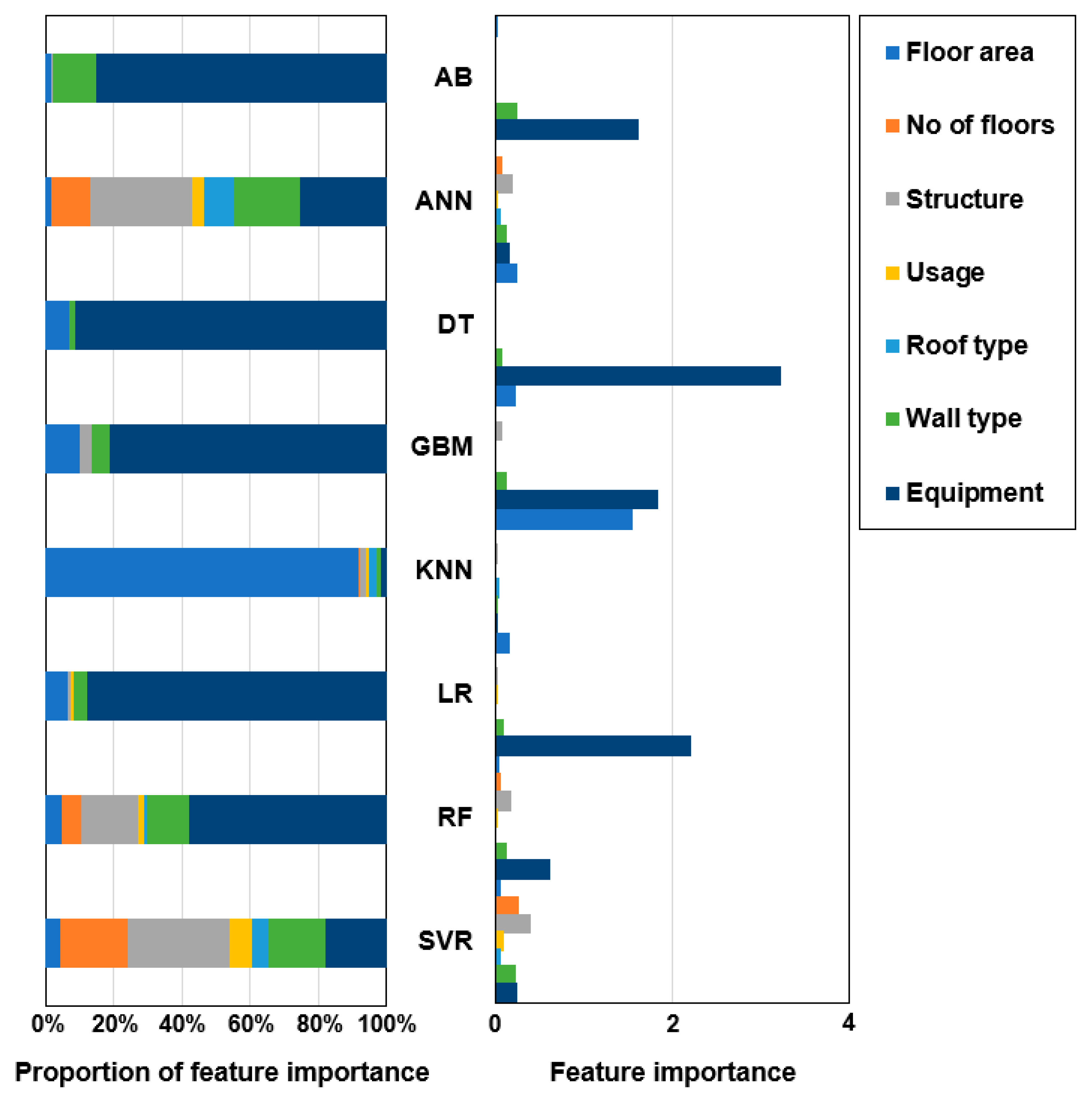
3.1. Feature Importance Analysis for Models

As for the importance of the features (i.e., input variables: floor area, structure, wall type, roof type, no. of floors, and equipment) used in the ML models developed to predict CO2 emissions at the building demolition stage, there are significant differences in the configuration and contribution of features for each model, as shown in Figure 3. The floor area is used as an important feature in almost all models. It particularly showed high importance in KNN (feature importance of floor area = 1.55), DT (feature importance of floor area = 0.24), and GBM (feature importance of floor area = 0.23). This indicates that the floor area is a key factor that has the largest impact on CO2 emissions. In addition, it is observed that equipment is used as an important feature in several models, including DT (feature importance of equipment = 3.23), LR (feature importance of equipment = 2.21), and GBM (feature importance of equipment = 1.84). However, the wall type and roof type show relatively low importance in most of the models.
The configuration of the feature group also varies depending on the model. The GBM model exhibits the highest prediction-performance results even though it predicted CO2 emissions at the demolition stage using only four features (floor area, structure, wall type, and equipment). The DT and AB models also showed high prediction-performance results using three and four features, respectively. The KNN, RF, and SVR models, however, reflect all of the seven features. The floor area, wall type, and equipment were used in all ML models. They can be considered important factors that affect CO2 emissions from buildings. In particular, the floor area and equipment are judged to be key features for most of the models, and the wall type was found to have a significant influence on the AB, ANN, and SVR models. Therefore, the most essential factors affecting CO2 emissions from buildings are judged to be the floor area and equipment among the seven features used in this study (i.e., floor area, structure, wall type, roof type, no. of floors, and equipment). Floor area serves as a key indicator of the scale of demolition work, as larger floor areas generally require increased equipment usage, longer working hours, and higher fuel consumption, ultimately leading to greater CO2 emissions. Additionally, equipment varies in fuel-consumption rates; for instance, crawler excavators and hydraulic breakers consume significantly more fuel compared to smaller machinery. The choice of equipment is determined by the building’s structure and material type, making it a primary factor influencing CO2 emissions. On the other hand, roof type or wall type reflects the specific characteristics of materials, but they do not directly determine equipment usage or work intensity. Therefore, their impact on CO2 emissions is relatively lower compared to floor area or equipment type.
These results show that an accurate understanding of the importance of features in ML models provides important insights into model selection and optimization strategies. For example, learning approaches can be used to predict CO2 emissions by focusing on specific features (i.e., equipment and floor area) using tree-based models (GBM, RF, and DT) or by creating various feature groups through nonlinear models (KNN and ANN). It is also possible to explore the possibility of improving the efficiency of models by properly tuning features with low importance (wall type and roof type). In this study, variables such as wall type and roof type were found to have low importance in predicting CO2 emissions, but they contribute to making the dataset more comprehensive and richer. These variables also provide opportunities to discover new patterns that could be utilized in future research or applications. While the overall impact of wall and roof type may be minor, they can serve as important data for studies focusing on recycling or assessing environmental impacts during the demolition process. In this regard, despite their low importance in CO2-emission prediction models, wall type and roof type can be considered meaningful input variables that can be applied to various research areas.

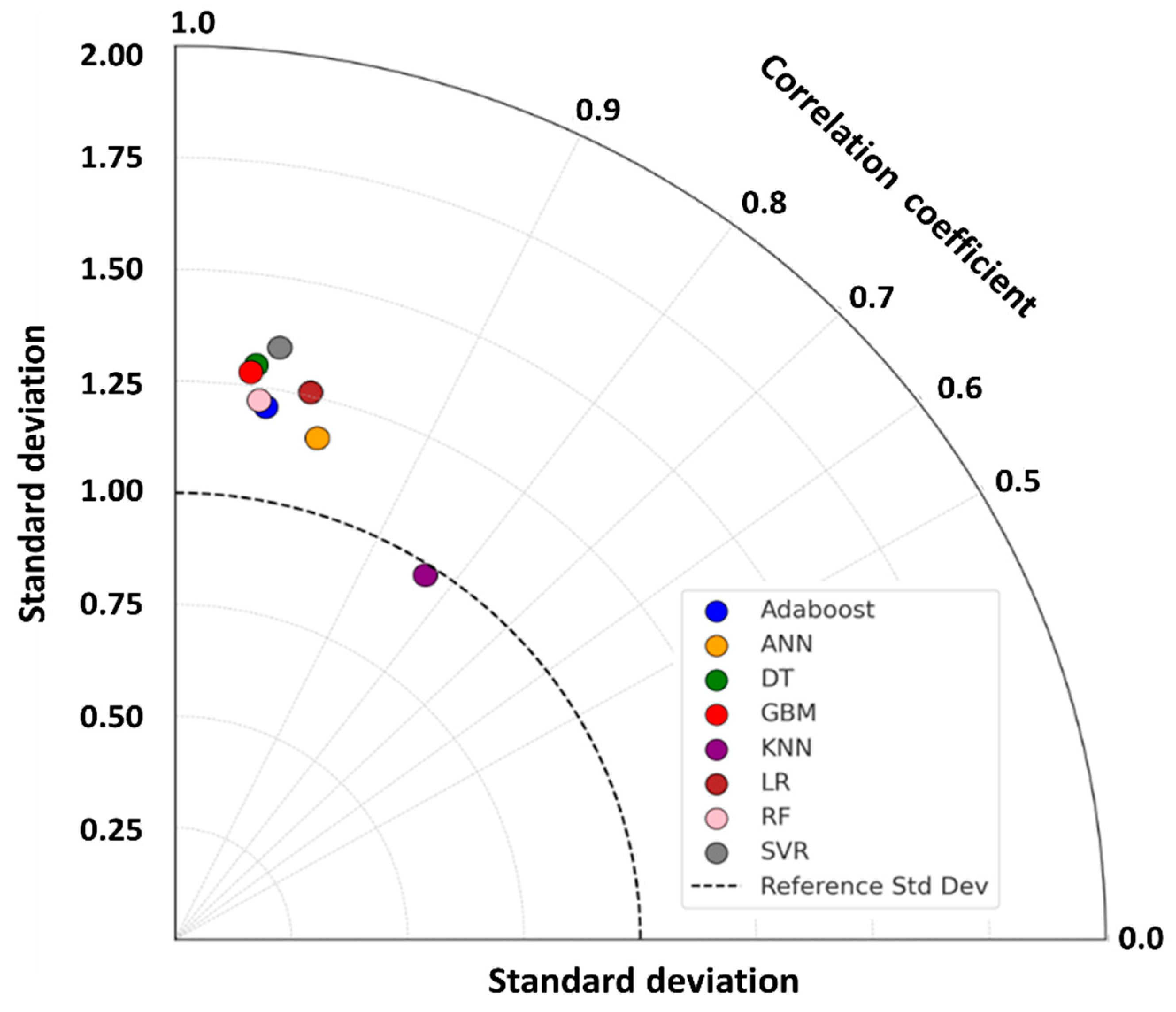
3.2. Comparison of the Performance of Prediction Models

Table 5 and Table 6 show the train, test, and validation performance results of the models developed in this study to predict CO2 emissions at the building demolition stage. For the training models, the RMSE, MAE, MAPE, and R-squared values of all models except for KNN showed high-performance results. In particular, the GBM (RMSE = 0.067, MAE = 0.045, MAPE = 0.098, R-squared = 0.997), DT (RMSE = 0.173, MAE = 0.079, MAPE = 0.115, R-squared = 0.983), and RF (RMSE = 0.103, MAE = 0.058, MAPE = 0.115, R-squared = 0.994) models showed low errors and high accuracy results. The AB, ANN, LR, and SVR models showed lower performance results in terms of errors and accuracy than the GBM, DT, and RF models. The KNN model was found to have the lowest CO2 emission prediction performance as it showed high errors and low explanatory power. For the test models, the GBM model also exhibited the highest prediction performance in all indicators, and the RF and DT models showed performance results close to the GBM model. The AB model is stable with low errors, but its explanatory power is somewhat insufficient in terms of accuracy. SVR exhibited low errors and high accuracy compared to the ANN, LR, and KNN models, but it showed somewhat larger errors and a lower R2 value than the GBM, RF, and DT models. The validation results are also similar to the train and test performance results, and the GBM model was found to be an excellent model that showed the highest performance in all indicators. In addition, the DT and RF models are also stable with lower RMSE and MAPE values, and they also have high R-squared values, indicating that they exhibit performance results close to GBM. Based on the performance metrics, the GBM model is estimated to be highly accurate in predicting CO2 emissions and effectively capable of learning the nonlinear relationships between input variables and CO2 emissions. The GBM model demonstrated its ability to handle the complex nonlinear relationships in the building demolition dataset and prioritize key variables, achieving high predictive accuracy. Therefore, selecting the GBM model as the benchmark is considered appropriate. In contrast, ANN and KNN exhibited lower performance due to the dataset size and high variability, while RF and DT showed relatively lower performance compared to GBM, as they lacked the ability to optimize the weights of weak learners effectively. These results suggest that the GBM model is particularly well suited for modeling the nonlinear relationships and handling the dataset size and variability in this study. In summary, the GBM model has the highest performance in predicting CO2 emissions at the building demolition stage, and the RF and DT models are judged to be stable models.
Figure 4 illustrates the Taylor diagram that compared the errors of CO2-prediction models with the observation data through the standard deviation and correlation coefficient. In the figure, the KNN model is close to the dotted line with a standard deviation of 1, thereby showing similar results to the observation data in terms of the standard deviation. Its performance of reproducing the CO2-emission pattern of the observation data, however, seems to be significantly insufficient due to the significantly low correlation coefficient of 0.835. In addition, the other models are distributed near a standard deviation of 1.25. In terms of the correlation coefficient, the GBM model (correlation coefficient = 0.992) is the closest to 1, indicating that it best reproduces the pattern of CO2 observation data. The DT (correlation coefficient: 0.991) and RF (correlation coefficient = 0.989) models were also found to be highly consistent with the observation data based on the correlation coefficient results. From Figure 4, GBM is identified as the best-performing model, as it demonstrates a high correlation coefficient and is positioned closest to the reference standard deviation, indicating its ability to effectively capture the actual patterns in the data. In contrast, KNN and ANN show lower predictive performance, making them unsuitable for complex problems such as CO2-emission predictions.
These train, test, and validation performance results from Table 5 and Table 6, and the Taylor diagram (Figure 4) show that the GBM model is the best for predicting CO2 emissions at the building demolition stage, and that the RF and DT models can also be considered stable in predicting CO2 emissions at the demolition stage.

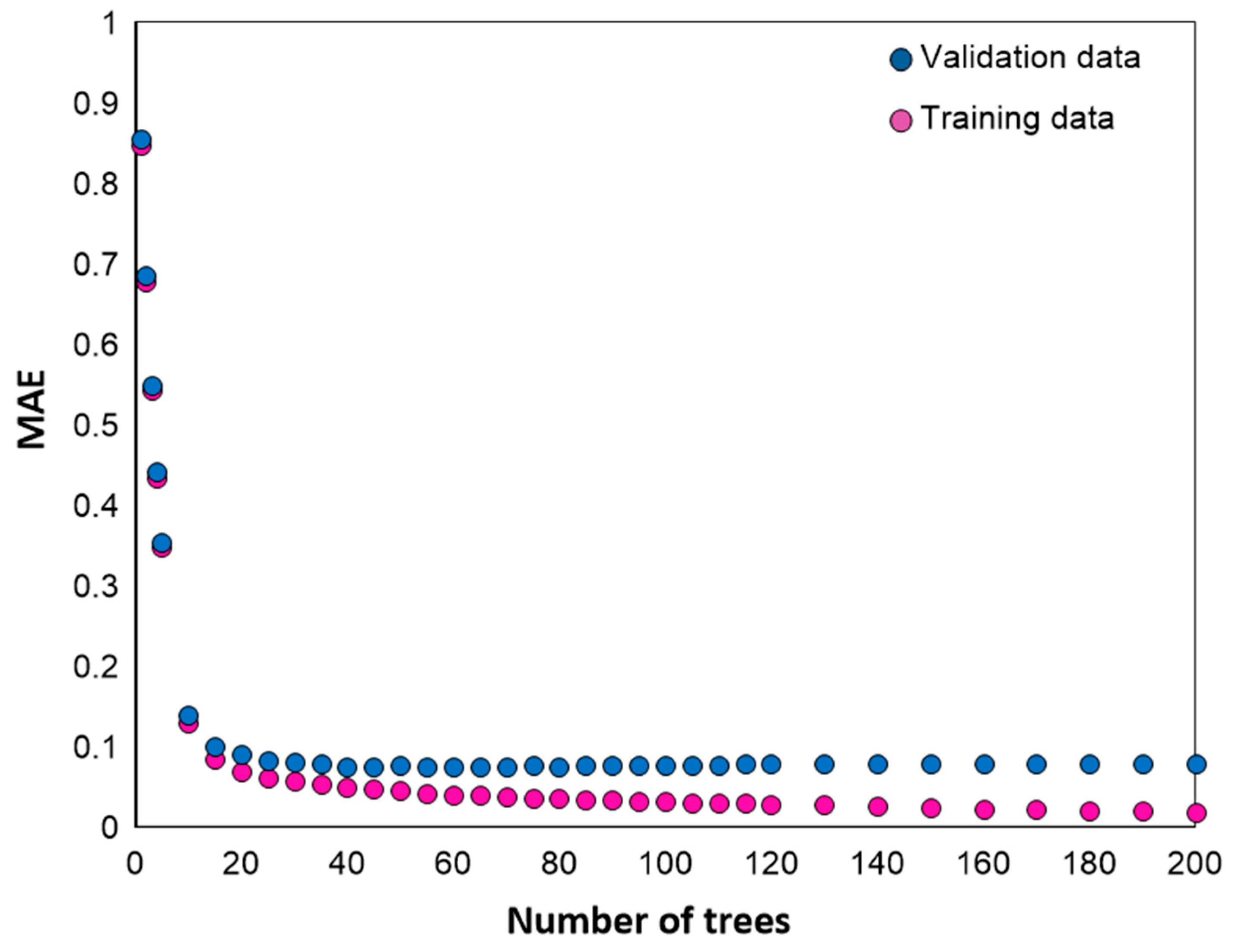
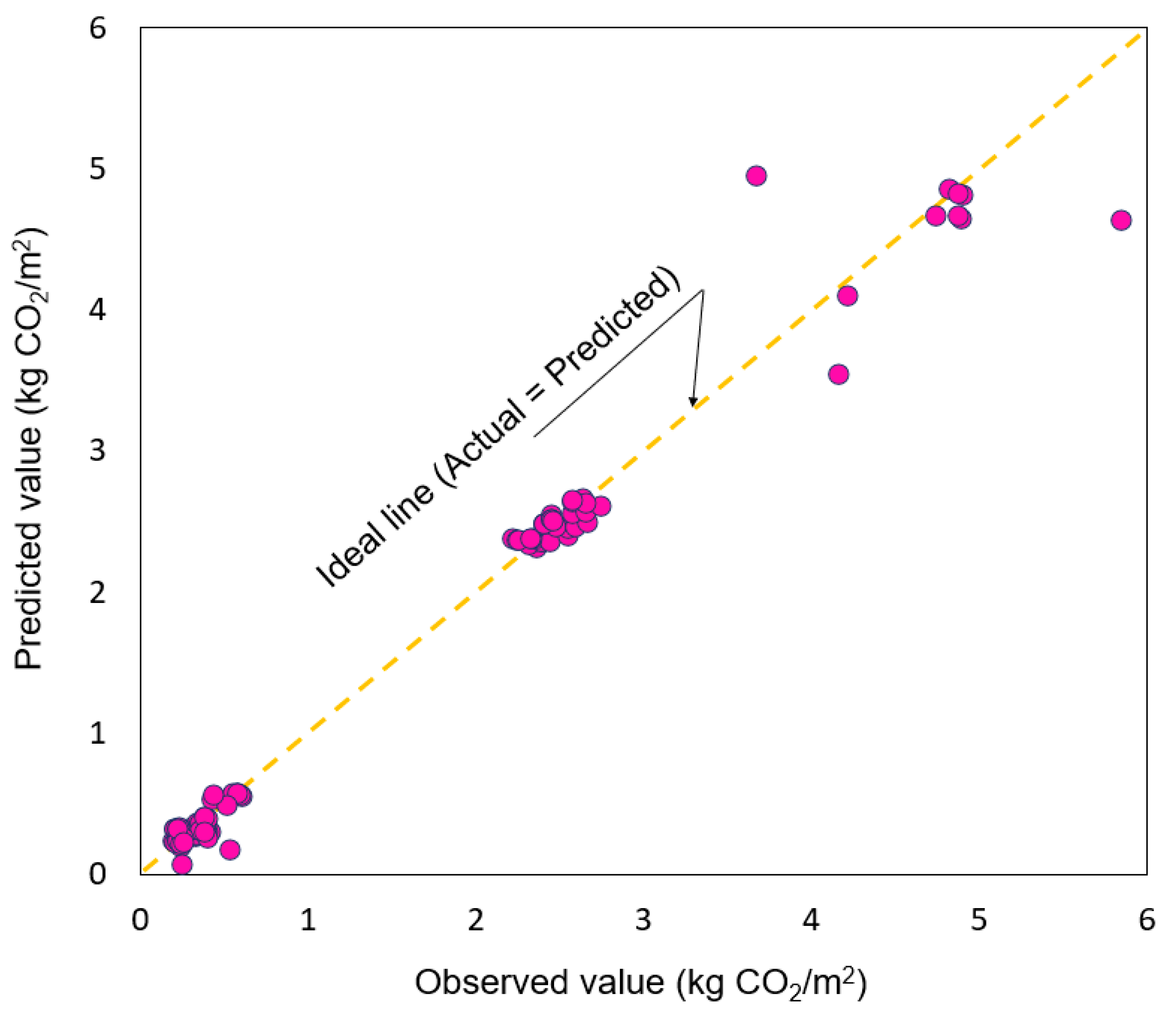
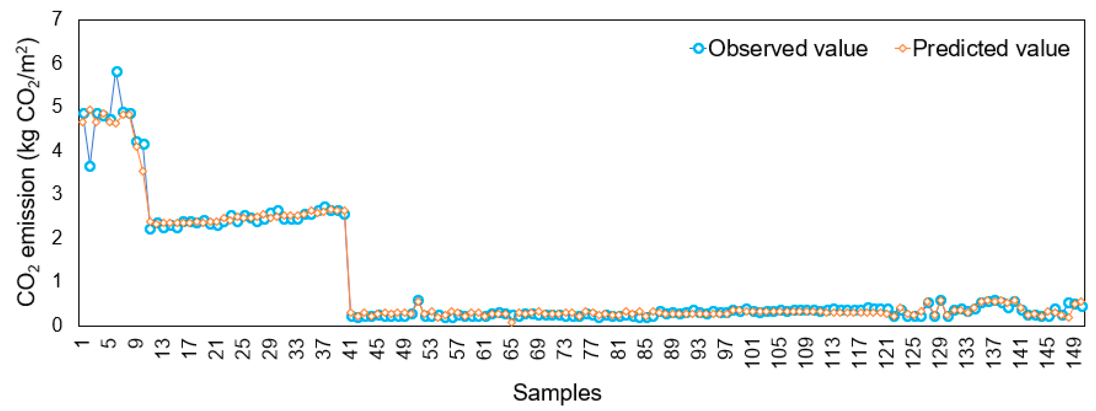
3.3. Generalization Performance and Accuracy of the Optimal Model for Predicting CO2 Emissions at the Demolition Stage

The developed GBM algorithm model was found to be optimal for CO2 prediction through high accuracy and low error results in all of the training, validation, and test steps. The errors and accuracy evaluation indicators of the model were examined in the previous section. In this section, the generalization performance of the GBM model was examined. For generalization-performance evaluation, LOSS evaluation was performed through residual analysis (Figure 5) and the MAE value. First, in the residual analysis graph in Figure 5, most residuals are concentrated within ±0.2, and they are symmetrically and randomly distributed with respect to zero. The average of the residuals is very small (0.0086). In addition, the histogram of the residuals seems to meet normality as it is symmetrically distributed and the central value is close to zero. These results indicate that the GBM model is not subjected to overfitting and has high generalization performance. Figure 6 shows the relationship between the MAE of training and validation data and the number of trees. It can be seen that MAE rapidly decreased and converged at certain levels (0.07 < MAE < 0.08, 20 ≤ number of trees ≤ 30) for both validation and training data. Specifically, the MAE of validation data was stabilized at a similar level to that of training data. This means that the model effectively learned the pattern of data without overfitting. From Figure 5, it can be observed that the GBM model is unbiased and accurately predicts most of the data, while Figure 6 demonstrates that the GBM model provides high generalization performance on validation data without overfitting. Therefore, this residual analysis (Figure 5) and LOSS curve (Figure 6) evaluation verify that the GBM algorithm provides high learning and generalization performance for the CO2-emission prediction problem.
Figure 7 shows the correlation between the observed values and the predicted values of the validation model. The correlation between the observed values and the predicted values of the GBM model was calculated to be close to 1 as the results were 0.999, 0.992, and 0.992 for the training, test, and validation data, respectively. As shown in Figure 7, most of the data are close to the ideal baseline (actual = predicted), confirming that the model has very high prediction accuracy. In addition, prediction performance with consistently high observed values was maintained, and generally high goodness of fit was observed except for one or two outliers. These results demonstrate that the GBM algorithm effectively learned the variability and pattern of data for the problem of predicting CO2 emissions at the building demolition stage. Therefore, from Figure 7, it can be concluded that the GBM model accurately predicted most of the data, demonstrating a high level of agreement with the actual values.
Figure 8 compares the observed and predicted values. High prediction accuracy is maintained in various sample sections, and the model exhibits high goodness of fit even in sections where the values sharply change. In this instance, the average observed and predicted values of the entire data are 1.037 (kg CO2/m2) and 1.028 (kg CO2/m2), respectively. The error is 0.83%, indicating the high accuracy of the GBM model. This finding verifies that the GBM model developed based on the data used in this study effectively learns the variability and pattern of the CO2 emission data of the building demolition stage and that it provides excellent generalization capability and reliable prediction performance.

4. Discussion

In previous studies on CO2 emissions at the building demolition stage in the building life cycle, research was mostly conducted based on LCA (Table 7). Quéheille et al. (2022) conducted research on CO2 emissions in the waste transport, waste processing, and waste disposal processes, including the demolition stage. In their study, CO2 emissions by the apartment building demolition scenario were found to be 2.13 (kg CO2/m2) [14]. Wang et al. (2018) conducted research on CO2 emissions at the demolition stage of high-rise residential buildings in Shenzhen, China based on LCA and reported the result of 8.7 GIA (1 m2 gross internal area) [38]. Ivanica et al. (2022) conducted research to construct a life cycle inventory at the demolition stage for five detached houses in Germany [7]. They reported that CO2 emissions at the building demolition stage ranged from 7.534 to 10.342 GIA. However, this study predicted CO2 emissions at the demolition stage using ML algorithms, showing that it is also possible to output CO2 emissions for the sub-features (i.e., reinforced concrete [RC], con-brick, masonry [block], and wood frame) of structures, that is, structure types, along with the average CO2 emissions of the observed and predicted values for the entire data. In Table 7, each study shows different results for CO2 emissions at the building demolition stage. This appears to be due to the system boundary of research, building types, and the characteristics of the equipment used. This study, however, shows CO2 emission results for various structures. While existing LCA models show the results of research cases specialized for certain building types, CO2-prediction models that use ML as in this study can present results for various building types. Therefore, it can be said that this scalability of ML models provides more benefits than previous studies on CO2 emissions based on LCA. It is also expected that ML models can be utilized for real-time prediction, reduction in the time required for data collection and analysis, and strategic plans for regions and projects.
Cases of using ML algorithms to predict CO2 emissions in the building life cycle can also be found in studies conducted for the construction stage and renovation stage (Table 8). Razi and Ansari. (2024) developed an ANN model with the highest performance in predicting CO2 emissions from construction projects by applying various ML algorithms [15]. The ANN model exhibited very high performance with R2 values of 0.995 and 0.978 in the training and test sets. Fang et al. (2021) developed a model for predicting CO2 emissions at the construction stage using RF [16]. The prediction performance of the RF model was not high with an R2 value of 0.640. In their study, only the RF and MLR algorithms were considered, and MLR showed even lower prediction performance than RF. Tsay et al. (2021) developed a GBM model to predict CO2 emissions from the building envelope renovation process. They considered only the GBM algorithm [39]. Nevertheless, the GBM model showed high prediction-performance results with R2 values of 0.993 and 0.989 in the training and test sets, respectively. In the cases of developing ML models for CO2 prediction in the building life cycle, GBM models exhibited powerful performance results in the study and Tsay et al. (2021) [39]. This indicates that it is also worth applying the GBM algorithm to research targeted at different system boundaries, such as the construction stage. Of course, for the development of ML models, deriving a model with optimal prediction performance by applying various ML algorithms should be considered first. This is because the development of CO2-prediction models for the building life cycle involves the selection of ML algorithms, system boundaries, and different characteristics of the data collected according to the setting of system boundaries as shown in Table 8. This means that ML algorithms need to be applied in a flexible manner according to various system boundaries and data characteristics. In addition, validation and generalization are required to improve the reliability of models.

5. Conclusions

In this study, ML models with optimal performance were developed and evaluated to predict CO2 emissions at the building demolition stage. Specifically, optimal feature sets and HPs were derived by applying various ML algorithms, and the optimal CO2-prediction model was derived from various ML models. The GBM model developed in this study for CO2 prediction exhibited the highest performance with R2 values of 0.997, 0.984, and 0.983 in the train, validation, and test data, respectively. It also showed high generalization performance. This indicates that the model can accurately predict CO2 emissions by effectively processing the nonlinear relationship and complexity of the data collected at the building demolition stage. The main findings and discussion points of this study are as follows:
  • ML models with high prediction and generalization performance for the building demolition stage were developed, and the GBM model exhibited the best performance. The GBM model showed high prediction performance for the demolition stage and other life cycle stages (e.g., renovation stage). It is expected that the model can be applied to various system boundaries for research on the environmental impacts of the building life cycle. The model is also expected to have much higher scalability compared to the existing LCA methodology in the efficient utilization of data, reduction in the time required for data collection and CO2 prediction, and strategic plans for projects;
  • When various algorithms were applied to predict CO2 emissions at the building demolition stage based on the data used in this study, it was found that the development of appropriate feature sets is important to ensure optimal performance for each algorithm. The GBM model with the highest performance in this study exhibited sufficiently high prediction-performance results using only four features (i.e., equipment, floor area, wall type, and structure). The DT model, which exhibited performance close to that of the GBM model, used only three features (i.e., equipment, floor area, and wall type). This indicates that accurately understanding the importance of features along with HP selection in ML models is important for model selection and optimization strategies;
  • Equipment was found to be a factor that has the largest effect on CO2 emissions at the building demolition stage, followed by the floor area, wall type, and structure. Equipment and the floor area were found to be key influence factors. This finding indicates that it is necessary first to consider variables, such as equipment and the floor area, for the development of models to predict CO2 emissions at the building demolition stage;
  • The findings of this study, as well as previous studies, show that it is necessary to fully consider various ML algorithms, system boundaries, and the characteristics of the data collected according to the setting of system boundaries in developing CO2-prediction models for the building life cycle. In addition, it is believed that a reliable model should be presented by adding the evaluation of validation and generalization performance along with the training and test results of the model.
The model developed in this study to predict CO2 emissions at the building demolition stage is expected to be utilized in carbon emission reduction plans by evaluating CO2 emissions in advance. It can also support eco-friendly design through CO2-emission prediction in the initial building design phase. Furthermore, it can also be utilized in the demolition stage CO2 reduction policy design as a tool to support policies and regulations, such as guidelines required to achieve carbon neutrality goals and setting of the carbon emission cap. For example, policymakers can use the GBM-based model to establish CO2-emission limits during building demolition or recommend the use of fuel-efficient equipment. Additionally, this can aid in implementing incentive programs, such as awarding subsidies for projects that achieve a reduction in CO2 emissions compared to the predicted levels. Practitioners can leverage GBM-based CO2-emission simulations for various equipment combinations and operating conditions to select equipment that minimizes CO2 emissions.
This study has certain limitations in several aspects. First, there are limitations in terms of system boundaries. As this study developed CO2 emission models with a focus on the demolition stage, the data range was limited, and subsequent processes (e.g., waste transport and disposal) were not included in the system boundary. To overcome the limitations of this study, it is necessary to expand the system boundary and construct a dataset accordingly. To achieve this, it is necessary to include data on vehicle information, fuel consumption, and transport distances related to waste transport, as well as studies on CO2 emissions based on waste types and disposal methods, such as landfilling, incineration, and recycling. In the future, it is deemed necessary to conduct research on ML models capable of comprehensive analysis by expanding the system boundary of the building life cycle. Second, there are limitations in the generalizability of the model due to the constraints of the data used. Since this study collected data from specific regions, it has limitations in terms of data scope, which may also restrict the generalization of the model. Additionally, the findings of this study are based on demolition scenarios within a specific region and may not fully account for differences in building materials, demolition methods, or energy consumption practices in other regions. To overcome these challenges, future research should expand the dataset to include a wider range of geographic regions and demolition methods. By doing so, the model can achieve greater applicability and contribute to more effective carbon reduction strategies across diverse contexts. Therefore, in the future, it will be necessary to expand data collection to cover a variety of regions and improve the model’s generalization performance based on this broader dataset.

Author Contributions

Conceptualization, methodology, validation, and supervision, G.-W.C.; resources, writing—review, editing, G.-W.C.; funding acquisition, C.-W.P. All authors have read and agreed to the published version of the manuscript.

Funding

This work was supported by the Commercialization Promotion Agency for R&D Outcomes (COMPA) grant funded by the Korean Government (Ministry of Science and ICT; RS-2023-00304695). This work was supported in part by the National Research Foundation of Korea (NRF) grant funded by the Korean government (MSIT; NRF-2022R1F1A107517313-1-3).

Data Availability Statement

The original contributions presented in the study are included in the article, further inquiries can be directed to the corresponding author.

Conflicts of Interest

The authors declare no conflict of interest.

Acronyms

ABAdaBoost
ANNartificial neural network
CDWconstruction and demolition waste
DTdecision tree
EoLend-of-life GBM, gradient boosting machine
HPhyper parameter
KNNK-nearest neighbors
LCAlife cycle assessment
LOOCVleave-one-out cross-validation LR, linear regression
MAEmean absolute error
MLmachine learning
R2coefficient of determination
RFrandom forest
RMSEroot mean square error
SVRsupport vector regression

References

  1. Kabir, M.; Habiba, U.E.; Khan, W.; Shah, A.; Rahim, S.; Rios-Escalante, P.R.D.l.; Farooqi, Z.-U.-R.; Ali, L.; Shafiq, M. Climate change due to increasing concentration of carbon dioxide and its impacts on environment in 21st century; a mini review. J. King Saud. Univ.-Sci. 2023, 35, 102693. [Google Scholar] [CrossRef]
  2. Li, R.; Kang, L.; Wu, S.; Zhou, X.; Wang, X. Effect of dust formation on the fate of indoor phthalates: Model analysis. Build. Environ. 2023, 229, 109957. [Google Scholar] [CrossRef]
  3. Webster, M.D.; Meryman, H.; Kestner, D.M. Carbon emissions and building structure: What the structural engineer needs to know about carbon in the 21st century. Proc. Struct. Congr. 2011, 2011, 472–482. [Google Scholar]
  4. He, W.; Li, W.; Xu, S.; Wang, W.; An, X. Time, cost, and energy consumption analysis on construction optimization in high-rise buildings. J. Constr. Eng. Manag. 2021, 147, 04021128. [Google Scholar] [CrossRef]
  5. Li, B.; Han, S.; Wang, Y.; Li, J.; Wang, Y. Feasibility assessment of the carbon emissions peak in China’s construction industry: Factor decomposition and peak forecast. Sci. Total Environ. 2020, 706, 135716. [Google Scholar] [CrossRef] [PubMed]
  6. Wu, Y.; Chau, K.W.; Lu, W.; Shen, L.; Shuai, C.; Chen, J. Decoupling relationship between economic output and carbon emission in the Chinese construction industry. Environ. Impact Assess. Rev. 2018, 71, 60–69. [Google Scholar] [CrossRef]
  7. Ivanica, R.; Risse, M.; Weber-Blaschke, G.; Richter, K. Development of a life cycle inventory database and life cycle impact assessment of the building demolition stage: A case study in Germany. J. Clean. Prod. 2022, 338, 130631. [Google Scholar] [CrossRef]
  8. Liu, J.; Huang, Z.; Wang, X. Economic and environmental assessment of carbon emissions from demolition waste based on LCA and LCC. Sustainability 2020, 12, 6683. [Google Scholar] [CrossRef]
  9. Cha, G.W.; Moon, H.J.; Kim, Y.C.; Hong, W.H.; Jeon, G.Y.; Yoon, Y.R.; Hwang, C.; Hwang, J.H. Evaluating recycling potential of demolition waste considering building structure types: A study in South Korea. J. Clean. Prod. 2020, 256, 120385. [Google Scholar] [CrossRef]
  10. Hao, J.L.; Ma, W. Evaluating carbon emissions of construction and demolition waste in building energy retrofit projects. Energy 2023, 281, 128201. [Google Scholar] [CrossRef]
  11. Peng, Z.; Lu, W.; Webster, C.J. Quantifying the embodied carbon saving potential of recycling construction and demolition waste in the Greater Bay Area, China: Status quo and future scenarios. Sci. Total Environ. 2021, 792, 148427. [Google Scholar] [CrossRef] [PubMed]
  12. Zhao, Q.; Gao, W.; Su, Y.; Wang, T.; Wang, J. How can C&D waste recycling do a carbon emission contribution for construction industry in Japan city? Energy Build. 2023, 298, 113538. [Google Scholar]
  13. Wu, H.; Zuo, J.; Zillante, G.; Wang, J.; Yuan, H. Status quo and future directions of construction and demolition waste research: A critical review. J. Clean. Prod. 2019, 240, 118163–118178. [Google Scholar] [CrossRef]
  14. Quéheille, E.; Ventura, A.; Saiyouri, N.; Taillandier, F. A life cycle assessment model of end-of-life scenarios for building deconstruction and waste management. J. Clean. Prod. 2022, 339, 130694. [Google Scholar] [CrossRef]
  15. Razi, N.; Ansari, R. A prediction-based model to optimize construction programs: Considering time, cost, energy consumption, and CO2 emissions trade-off. J. Clean. Prod. 2024, 445, 141164. [Google Scholar] [CrossRef]
  16. Fang, Y.; Lu, X.; Li, H. A random forest-based model for the prediction of construction-stage carbon emissions at the early design stage. J. Clean. Prod. 2021, 328, 129657. [Google Scholar] [CrossRef]
  17. Akanbi, L.A.; Oyedele, A.O.; Oyedele, L.O.; Salami, R.O. Deep learning model for demolition waste prediction in a circular economy. J. Clean. Prod. 2020, 274, 122843. [Google Scholar] [CrossRef]
  18. Cha, G.W.; Moon, H.J.; Kim, Y.C. A hybrid machine-learning model for predicting the waste generation rate of building demolition projects. J. Clean. Prod. 2022, 375, 134096. [Google Scholar] [CrossRef]
  19. Guerra, B.C.; Koo, H.J.; Caldas, C.; Leite, F. Prediction of waste diversion and identification of trends in construction and demolition waste data using data mining. Int. J. Constr. Manag. 2024, 24, 374–383. [Google Scholar] [CrossRef]
  20. Gulghane, A.; Sharma, R.L.; Borkar, P. A formal evaluation of KNN and decision tree algorithms for waste generation prediction in residential projects: A comparative approach. Asian J. Civ. Eng. 2024, 25, 265–280. [Google Scholar] [CrossRef]
  21. Hu, R.; Chen, K.; Chen, W.; Wang, Q.; Luo, H. Estimation of construction waste generation based on an improved on-site measurement and SVM-based prediction model: A case of commercial buildings in China. Waste Manag. 2021, 126, 791–799. [Google Scholar] [CrossRef]
  22. Lu, W.; Long, W.; Yuan, L. A machine learning regression approach for pre-renovation construction waste auditing. J. Clean. Prod. 2023, 397, 136596. [Google Scholar] [CrossRef]
  23. Maged, A.; Elshaboury, N.; Akanbi, L. Data-driven prediction of construction and demolition waste generation using limited datasets in developing countries: An optimized extreme gradient boosting approach. Environ. Dev. Sustain. 2024, 1–25. [Google Scholar] [CrossRef]
  24. Cha, G.W.; Park, C.W.; Kim, Y.C.; Moon, H.J. Predicting Generation of Different Demolition Waste Types Using Simple Artificial Neural Networks. Sustainability 2023, 15, 16245. [Google Scholar] [CrossRef]
  25. Cha, G.W.; Park, C.W.; Kim, Y.C. Optimal Machine Learning Model to Predict Demolition Waste Generation for a Circular Economy. Sustainability 2024, 16, 7064. [Google Scholar] [CrossRef]
  26. Mallikharjuna Rao, K.; Saikrishna, G.; Supriya, K. Data preprocessing techniques: Emergence and selection towards machine learning models—A practical review using HPA dataset. Multimed. Tools Appl. 2023, 82, 37177–37196. [Google Scholar] [CrossRef]
  27. Xu, X.; Chong, W.; Li, S.; Arabo, A.; Xiao, J. MIAEC: Missing data imputation based on the evidence chain. IEEE Access 2018, 6, 12983–12992. [Google Scholar] [CrossRef]
  28. Liu, X.; Wang, H. A discretization algorithm based on a heterogeneity criterion. IEEE Trans. Knowl. Data Eng. 2005, 17, 1166–1173. [Google Scholar] [CrossRef]
  29. Seyedzadeh, S.; Rahimian, F.P.; Glesk, I.; Roper, M. Machine learning for estimation of building energy consumption and performance: A review. Vis. Eng. 2018, 6, 5. [Google Scholar] [CrossRef]
  30. Gao, Y.; Wang, J.; Xu, X. Machine learning in construction and demolition waste management: Progress, challenges, and future directions. Autom. Constr. 2024, 162, 105380. [Google Scholar] [CrossRef]
  31. Abdallah, M.; Talib, M.A.; Feroz, S.; Nasir, Q.; Abdalla, H.; Mahfood, B. Artificial intelligence applications in solid waste management: A systematic research review. Waste Manag. 2020, 109, 231–246. [Google Scholar] [CrossRef] [PubMed]
  32. Cha, G.W.; Moon, H.J.; Kim, Y.C. Comparison of random forest and gradient boosting machine models for predicting demolition waste based on small datasets and categorical variables. Int. J. Environ. Res. Public Health 2021, 18, 8530. [Google Scholar] [CrossRef] [PubMed]
  33. Lu, W.; Lou, J.; Webster, C.; Xue, F.; Bao, Z.; Chi, B. Estimating construction waste generation in the Greater Bay Area, China using machine learning. Waste Manag. 2021, 134, 78–88. [Google Scholar] [CrossRef] [PubMed]
  34. Ali, Y.A.; Awwad, E.M.; Al-Razgan, M.; Maarouf, A. Hyperparameter search for machine learning algorithms for optimizing the computational complexity. Processes 2023, 11, 349. [Google Scholar] [CrossRef]
  35. DeCastro-García, N.; Munoz Castaneda, A.L.; Escudero Garcia, D.; Carriegos, M.V. Effect of the sampling of a dataset in the hyperparameter optimization phase over the efficiency of a machine learning algorithm. Complexity 2019, 2019, 6278908. [Google Scholar] [CrossRef]
  36. Cheng, J.; Dekkers, J.C.; Fernando, R.L. Cross-validation of best linear unbiased predictions of breeding values using an efficient leave-one-out strategy. J. Anim. Breed. Genet. 2021, 138, 519–527. [Google Scholar] [CrossRef] [PubMed]
  37. Rani, R.; Arora, G. A comparative study of PSO and LOOCV for the numerical approximation of sine–gordon equation with exponential modified cubic B-Spline DQM. Oper. Res. Forum. 2024, 5, 89. [Google Scholar] [CrossRef]
  38. Wang, J.; Wu, H.; Duan, H.; Zillante, G.; Zuo, J.; Yuan, H. Combining life cycle assessment and Building Information Modelling to account for carbon emission of building demolition waste: A case study. J. Clean. Prod. 2018, 172, 3154–3166. [Google Scholar] [CrossRef]
  39. Tsay, Y.S.; Yeh, C.Y.; Chen, Y.H.; Lu, M.C.; Lin, Y.C. A machine learning-based prediction model of lcco2 for building envelope renovation in taiwan. Sustainability 2021, 13, 8209. [Google Scholar] [CrossRef]
Figure 1. Research flowchart for development of CO2-emission prediction model in demolition stage.
Buildings 15 00526 g001
Figure 2. Distribution of CO2 emissions by building floor area.
Buildings 15 00526 g002
Figure 3. Comparative analysis of feature importance for CO2-emission prediction by ML models.
Buildings 15 00526 g003
Figure 4. Taylor diagram for comparison of CO2-emission prediction models.
Buildings 15 00526 g004
Figure 5. Residual plot and distribution of predicted and observed values by the GBM model.
Buildings 15 00526 g005
Figure 6. MAE progression of the training and validation data as a function of the number of trees.
Buildings 15 00526 g006
Figure 7. Correlation between observed and predicted values of CO2 prediction model by GBM algorithm.
Buildings 15 00526 g007
Figure 8. Comparison of observed and predicted values of CO2 emission by GBM algorithm.
Buildings 15 00526 g008
Table 1. Parameters, units, and sources collected for this study.
Parameter Unit SourceComment
CharacteristicDetailed Characteristic
Floor area m2On-site measurementsCheck the dimensions by measuring with a laser measuring device by two people on-site
Usage Residential
Residential and commercial
-Documents and observationsConfirm building ledger document
Structure Reinforced concrete
Concrete-brick
Masonry-block
Wood
-Documents and observationsConfirm building ledger document
Wall typeConcrete
Brick
Bock
Mud-plastered and mortar
-ObservationsCheck through on-site observation
Roof typeSlab
Slab and roofing tile
Slate
Roofing tile
-ObservationsCheck through on-site observation
Number of floors FloorObservationsCheck through on-site observation
Equipment typeA type
B type
C type
PieceObservations and inquiryCheck the type of equipment used and work capability
Energy consumption L/m2InquiryContact the company
Table 2. Statistical analysis of fuel consumption and CO2-emission data after data preprocessing.
ClassificationMinMaxMeanMedianStandard DeviationVariance
Diesel consumption (L)4.37364.2974.4612.96106.7811,401.05
Diesel-consumption rate(L/m2)0.082.250.40.140.50.25
CO2 emission (kg-CO2)11.36947.15193.5933.69277.6277,071.12
CO2-emission rate (kg-CO2/m2)0.25.841.040.361.311.72
Table 3. Description of various machine learning algorithms utilized in this study.
Machine Learning AlgorithmDescription
Adaboost (AB)AdaBoost, a meta-estimator, first performs the learning of the regression model using the original dataset and then the learning of the additional regression model copy using the same dataset with adjusted weights of each instance according to the error of the current prediction.
Artificial Neural Networks (ANN)ANN is a computing system composed of multiple layers (input–hidden–output) and neurons. The basic structure of ANN consists of three layers (i.e., input, hidden, and output), and nonlinear transfer functions that allow the learning of nonlinear and linear relationships between input and output neurons constitute several layers of neurons.
Decision tree (DT)The DT algorithm, a supervised learning model to deal with classification and regression problems, is used to efficiently extract a set of rules from unfamiliar data.
Gradient boosting machine (GBM)GBM, one of the most robust ML algorithms, has been widely applied in engineering fields, and it corresponds to the boosting technique. This algorithm creates strong learners by continuously adding weak learners to the model. It improves the performance of the model and minimizes the loss or error of the model by repeatedly integrating various predictor variables.
K-nearest neighbor (KNN)KNN is a simple and easy-to-implement supervised learning method used for classification and regression problems. This method uses training data and distance calculation for the pre-defined k value, and finds k closest values using the clustering algorithm.
Linear regression (LR)LR is a regression model that estimates the relationship between one independent and one dependent variable using a straight line.
Random forest (RF)RF is a bagging-based representative ensemble technique that generates bootstrap sampling. It creates a tree for each subset by extracting several subsets from the original dataset. Strong learners are determined through a majority vote on the results of each tree, and the final prediction is based on the average prediction of all submodels.
Support vector regression (SVR)SVR uses the same principle as the support vector machine (SVM). Its basic concept is to find the line of best fit. The line of best fit indicates a hyperplane that contains as many data points as possible.
Table 4. HP configuration for developing optimized CO2 emission prediction models by algorithm.
AlgorithmsHP TitleTested HP and ValuesSelected HP
ABNo. of estimatorsx ∈ {5, 10, 15, …, 150}30
Learning ratex ∈ {0.0001, 0.001, 0.01, 0.1, 0.2, 0.3, …, 1}1
Loss (regression)Linear, square, exponentialLinear
ANNActivation functionReLu, tanh, logistic, identity ReLu
No. of neuronsx ∈ {1, 2, 3, 4, 5, 6, 7, …, 60}5
SolverL-BFGS-B, SGD, AdamL-BFGS-B
Regularizationx ∈ {0.0001, 0.001, 0.01, 0.1, 10, 20, 30, 40, …, 100, 1000}30
Iterationx ∈ {10, 20, 30, …, 150}10
DTMin_samples_splitx ∈ {1, 2, 3, …, 10}6
Criterionx ∈ {1, 2, 3, …, 10}1
Max_depth x ∈ {1, 2, 3, …, 15}3
GBMNo. of treesx ∈ {5, 10, 15, …, 150}40
Criterionx ∈ {1, 2, 3, …, 10}2
Max_depthx ∈ {1, 2, 3, …, 15}2
Learning ratex ∈ {0.001, 0.01, 0.1, 0.2, 0.3, …, 1}0.2
KNNNo. of neighborsx ∈ {1, 2, 3, …, 15}3
MetricEuclidean, Manhattan, Chebyshev, mahalanobisManhattan
WeightUniform, by distancesBy distances
LRRegularization methodRidge, lasso, elastic netElastic net
L1:L2x ∈ {0.1, 0.2, 0.3, …, 1}0.8:0.2
Regularization   ( α ) x ∈ {0.0001, 0.001, 0.01, 0.1, 1, 10, 100, 1000}0.001
RFNo. of treesx ∈ {5, 10, 15, …, 150}60
Criterionx ∈ {1, 2, 3, …, 10}6
Max_depthx ∈ {1, 2, 3, …, 15}5
Max_featuresx ∈ {1, 2, 3, 4, 5, 6, 7}2
SVRRegression Costx ∈ {0.1n∣n ∈ {1, 2, …, 10}} ∪ {n∣n ∈ {1, 2, …, 10}} ∪ {10n∣n ∈ {1, 2, …, 10}}0.9
Regression loss epsilonx ∈ {0.1n∣n ∈ {1, 2, …, 10}} ∪ {n∣n ∈ {1, 2, …, 10}} ∪ {10n∣n ∈ {1, 2, …, 10}}0.5
Kernel typeLinear, RBF, polynomial, sigmoidPolynomial
Gammax ∈ {0.01, 0.05, 0.1, 0.15, …, 0.95, 1.0}1
Coefficientx ∈ {0.01, 0.05, 0.1, 0.15, …, 0.95, 1.0}0.01
Degreex ∈ {1, 2, 3, …, 10}2
Table 5. Training and test performance of ML models for predicting CO2 emissions in building demolition stage.
AlgorithmTrainingTest
RMSEMAEMAPER-SquaredRMSEMAEMAPER-Squared
AB0.2130.0730.1240.9730.2130.0740.1240.973
ANN0.2840.1770.3090.9530.3560.1970.2890.926
DT0.1730.0790.1150.9830.1550.0690.1050.986
GBM0.0670.0450.0980.9970.1690.0750.1290.983
KNN0.6980.2050.1690.7160.7460.2240.2750.653
LR0.2630.1810.3410.9600.3210.2020.3500.940
RF0.1030.0580.1150.9940.2210.0970.1800.977
SVR0.2110.1080.1490.9740.2820.1520.2670.954
Table 6. Validation performance of ML models for predicting CO2 emissions in building demolition stage.
ML AlgorithmValidation
RMSEMAEMAPER-Squared
AB0.2130.0750.1410.972
ANN0.3540.2140.3740.927
DT0.2250.0870.1150.970
GBM0.1650.0710.1270.984
KNN0.7430.2370.2240.677
LR0.3030.1990.3610.946
RF0.2270.1010.1960.970
SVR0.2710.1650.3260.957
Table 7. Comparison of studies on CO2 emissions in the demolition stage of building.
Reference System BoundaryStructureCO2 Emission (kg CO2/m2)
ObservedPredicted
This studyDemolition stageReinforced concrete4.6964.570
Con-brick2.461 2.469
Masonry (block)0.292 0.289
Wood0.382 0.383
Average of all data1.0371.028
Ivanica et al., 2022 [7]Demolition, waste sorting, and loading stageconcrete-brick
concrete-block
7.534–10.342 GIA
Quéheille et al., 2022 [14]Demolition stageMetal frame2.13 *
Wang et al., 2018 [38]Demolition stageReinforced concrete
(high-rise residential building)
8.7 GIA
* In the study by Quéheille et al. (2022) [14], the energy consumption for the demolition stage (diesel, unit: liters) and the net area (m2) were used to estimate CO2 emissions based on the diesel emission factor of 2.6 kg CO2/liter from the IPCC 2006 guidelines.
Table 8. Comparison of studies on optimal ML model development for CO2 prediction in end-of-life cycles.
ReferenceOptimal AlgorithmSystem BoundaryPerformance (R2)
This studyGBMDemolition stageTraining 0.997
Test 0.983
Validation 0.984
Razi and Ansari. (2024) [15]ANNConstruction stageTraining 0.9949
Test 0.9799
Fang et al. (2021) [16]RFConstruction stageTraining 0.6403
Tsay et al. (2021) [39]GBMRenovation stageTraining 0.993
Test 0.989
Disclaimer/Publisher’s Note: The statements, opinions and data contained in all publications are solely those of the individual author(s) and contributor(s) and not of MDPI and/or the editor(s). MDPI and/or the editor(s) disclaim responsibility for any injury to people or property resulting from any ideas, methods, instructions or products referred to in the content.

