Finite Element Method Analysis of Seismic Response of Confined Masonry Walls with Openings Built Using Polyurethane Glue

Abstract

The seismic response of confined masonry (CM) walls, built from innovative hollow clay blocks featuring large thermal insulation cavities and bonded with polyurethane glue instead of thin-layer mortar, was investigated. A 3D micro-model was subsequently developed in Abaqus and validated against results from cyclic shear tests on full-scale CM wall specimens. Once validated, the model was utilized in an extensive parametric study to investigate the effects of openings on the walls. This parametric study considered the size of the opening, its position, the aspect ratio of the walls, and different sizes of tie-columns. The results showed that the size and placement of openings substantially and negatively affected seismic response, and that the detrimental effects can be alleviated by placing strong tie-columns next to the openings.

1. Introduction

In the past couple of decades, research in the field of masonry in Europe has been focused on improving the thermal properties of masonry. Consequently, new materials and techniques have been developed, one of which is the use of hollow clay blocks with enlarged cavities, which are specifically designed to enhance thermal insulation and reduce energy consumption for heating and cooling. When such units are used in combination with a new adhesive (i.e., polyurethane (PU) glue) instead of traditional thin-bed mortar, they have near-zero-thickness joints, which minimize thermal losses and allow for faster construction.

A confined masonry (CM) system, which consists of load-bearing masonry walls enclosed on all four sides by cast-in-place reinforced concrete (RC) tie-columns and tie-beams, offers an effective solution for enhancing the structural performance of masonry buildings, particularly in seismic-prone areas across the world. Although the basic concept of CM is the same everywhere, there are important differences between regions. For example, the typical thickness of CM walls in Mexico, as tested by, e.g., Perez Gavilan et al. [1], is only 12 cm, while in Chile, the typical wall thickness is 15 cm [2]. Eurocode 8 [3] specifies a minimum masonry wall thickness of 24 cm, whereas the blocks examined in this study have a thickness of 38 cm. European blocks also have a much larger share of holes compared to other regions. The differences in wall thickness between different regions are significant, and when walls are thick, confining is trickier. From the perspective of structural strength, confinement is most effective when tie-columns cover the entire thickness of the wall. However, this may not always be practical.

In Europe, tie-columns should have a minimum dimension of 15 cm (Eurocode 8 [3]), which is much less than the required 24 cm thickness of walls, which indicates that different widths of tie-columns and walls are normal. In other countries too, the smallest tie-column cross-section ranges from 10 to 20 cm (Marques and Lourenço [4]), which is often less than the required width of the wall. This is allowed because tie-columns can provide sufficient confinement even if they are smaller. Moreover, the disparity between the thickness of tie-columns and walls enables thicker thermal insulation of tie-columns, which present thermal bridges. In addition, by decreasing the dimensions of tie-columns, concrete consumption can be significantly minimized, especially since there can be quite a lot of tie-columns in a structure.

The considered masonry has tie-columns with dimensions of 25 × 25 cm, which is 13 cm less than the thickness of the wall (38 cm). The tie-columns are placed so that one surface is flush with the masonry, while the other is depressed by 13 cm. The masonry blocks in contact with the depressed side of the tie-columns are therefore locally stressed, and recent tests on two CM walls [5] have revealed that a specific type of damage develops at the point of contact with the tie-column.

There are different numerical modelling strategies for the seismic analysis of CM structures, as recently presented in Marques et al. [6] and Borah et al. [7]. Most typically, the Finite Element Method (FEM) is used for modelling, but the approaches based on FEM (micro, simplified micro, or macro approach) vary in terms of their refinement and capability to capture failure modes and seismic response. Recent publications have shown that the most commonly used FE softwares for the analysis of CM are DIANA [8] and Abaqus [9]. Additionally, ANSYS software has been widely used for the modelling and analysis of unreinforced masonry (URM) [10]. Typically, 2D models are preferred, as they can accurately simulate in-plane responses and are usually sufficient to capture the key phenomena in CM walls, specifically in RC ties and along the interface between the tie-column and masonry. However, 3D models are employed when specific structural effects need to be considered, as demonstrated in studies such as that by Chourasia et al. [11]. Given the unique nature of the shear damage observed at the interface of the tie-column and masonry in this study, the use of a 3D FE model was necessary. In addition to the necessity of using a full 3D FE model, detailed material models require a significant amount of input data for the materials and different types of contacts. Due to the inherent brittleness of both concrete and masonry [12], considerable effort was made to gather and record the necessary material and contact properties. These parameters were primarily derived from dedicated tests conducted on the structural elements, materials, and joints [5,13]. Additionally, the FE model was validated by comparing it against two experimental tests that evaluated the pushover response and damage patterns, following a methodology similar to that used by Marques et al. [6] in DIANA software and Tripathy and Singhal [14] in Abaqus software.

In addition to FEM, the Applied Element Method (AEM) is an alternative for structural analysis, which is particularly useful in simulating the collapse behaviour of masonry structures. Some decades ago, AEM was introduced as a discrete modelling technique [15], whereby structures are divided into small elements connected by normal and shear springs. These springs simulate stresses and deformations due to loading, allowing the model to capture failure mechanisms as the structure progresses from cracking to complete separation. While FEM remains the predominant method in seismic analysis, AEM offers advantages, especially in modelling collapse scenarios and debris generation, as demonstrated in a study by Domaneschi [16].

This parametric study systematically investigates the seismic response of CM walls with openings, focusing on the influence of wall geometry (aspect ratio-AR), opening size, position, and shape (solid, window, or door), as well as the presence and size of tie-columns around these openings. The lack of such confining elements around large openings has been linked to significant damage in CM walls during past earthquakes [17,18]. Furthermore, this study examines two different approaches for the placement of RC confining elements around openings. The first is based on recommendations by Brzev and Mitra [19] and international guidelines [17], which suggest that vertical tie-columns should be positioned on both sides of any opening exceeding 10% of the CM wall’s surface area; otherwise, the wall cannot be considered as a CM wall for seismic design. In contrast, the second approach, as outlined in Eurocode 8 [3], stipulates that vertical confining elements should be placed on both sides of any opening with an area greater than 1.5 m². By comparing these two approaches, this study aims to assess their effectiveness in enhancing the seismic performance of CM walls with various opening configurations.

There is a clear need for further research to address gaps in understanding of how openings affect the seismic performance of CM walls. While it is well known that openings reduce the strength and deformation capacity of these walls, few studies have examined the influence of different opening configurations and the presence of confining elements around them. Following the conclusions of Perez Gavilan et al. [20], future research should focus on the in-plane behaviour of CM walls with openings, considering different sizes and locations of openings, with an emphasis on verifying the effect of the size of RC confining elements. Comprehensive numerical investigations are crucial to assess these factors, with the primary aim being the development of reliable and accurate FE models, as full-scale experiments are often costly and challenging to conduct.

In recent decades, several experimental studies have been conducted to investigate the seismic behaviour of CM walls with openings. Experimental research by Yanez et al. [21] revealed that larger openings (over 25% of the CM wall area) led to a 40–50% reduction in strength compared to the corresponding solid specimens, while smaller openings (up to 11% of the CM wall area) had no significant effect on stiffness. Similarly, Kuroki et al. [22] found that unconfined openings caused a 15–40% reduction in shear resistance, with centrally located openings being less affected than eccentric ones. The results also stated that CM walls with both vertical and horizontal confining elements exhibited improved strength, but experienced a reduction in ductility, compared to CM walls with openings confined only by vertical RC tie-columns.

Recently, an experimental study by Gupta and Singhal [23] evaluated the effects of openings in CM walls and the role of confining elements around these openings. The study found that walls with unconfined openings experienced strength reductions of 31% to 49%, while the addition of RC confining elements improved in-plane capacity by 36% to 130%. Additionally, a confinement factor was introduced to quantify the contribution of these confining elements, allowing for more accurate strength estimations for CM walls with confinement around the openings.

Okail et al. [24] conducted a comprehensive experimental and numerical investigation on CM walls, examining the effects of various parameters, such as opening size, position, aspect ratio, axial load, and longitudinal reinforcement in tie-columns, on the lateral load response. Their findings highlighted that larger openings significantly reduced the lateral load capacity of the walls. However, confining elements, particularly tie-columns around openings, were shown to effectively restore this lost capacity and enhance ductility. These results emphasize the importance of incorporating confining elements to maintain strength and improve the deformation capacity of walls with openings under seismic loading.

In addition to these experimental insights, several studies have focused on the numerical investigation of CM walls with openings. Maheri et al. [25] conducted 18 numerical analyses of CM walls with door openings, considering aspect ratios of 0.5, 1.0, and 2.0, as well as two different masonry compressive strengths (2.0 MPa and 5.0 MPa). Their findings revealed that the size of the opening, particularly the ratio of opening length to wall length (OL/WL), significantly influenced the shear and flexural responses of the walls. As the opening size increased, especially in walls with higher aspect ratios, a notable reduction in shear capacity was observed.

Shandilya et al. [26] highlighted the significant influence of the window opening size and the shape of openings on the seismic performance of CM walls with rectangular (AR = 0.75) and square (AR = 1) configurations. Increasing the opening size (from 10% to 60%) resulted in a considerable reduction in both ultimate strength and stiffness. For a CM wall with AR = 0.75, the ultimate strength decreased by approximately 30% to 80%, while stiffness was reduced by 55% to 95%. In contrast, for a CM wall with AR = 1.0, strength reductions ranged from 33% to 89%, and stiffness decreased by between 30% and 96%. The study found that both the shape and size of openings significantly affect the strength and energy dissipation capacity of these walls, with larger openings reducing their ability to withstand seismic forces.

Section 2 describes the materials and the results of shear compression tests from the literature. Section 3 focuses on the description of the numerical model developed in Abaqus software, and the validation of the model with experiments. In Section 4, the results of the comprehensive parametric study are presented, followed by a brief conclusion.

2. Brief Overview of Past Experimental Study

The masonry blocks used in the previous experimental study [5] were vertically perforated, commercially available units, designed for constructing thermally efficient 38 cm thick walls. Their nominal dimensions were 250 mm in length, 249 mm in height, and 380 mm in thickness, as shown in Figure 1a. The blocks and their mechanical properties have been extensively tested and thoroughly evaluated in a prior study by Gams et al. [5].

The mean compressive strength of the blocks $f_m$ was measured to be 11.4 MPa, while the normalized mean strength $f_b$ was 13.1 MPa. The results from material characterization tests indicated that the masonry compressive strength $f_m$ aligned with the strength predicted by Eurocode 6 [27] for masonry hollow clay blocks with traditional thin-bed mortar, confirming the material’s expected performance. To enhance damage observation during testing, the thermal insulation filling the large cavities of the units (Figure 1a) was removed, as shown in Figure 1b. Given its negligible stiffness and strength, its removal did not influence the mechanical behaviour of the masonry wall, as noted in [5].

For the masonry wall construction, a new adhesive PU glue was applied on blocks without mineral wool in four strips along the width of the units (Figure 1b). This adhesive was specifically chosen to enhance the thermal efficiency of the masonry wall by minimizing the thickness of the bed-joints. The masonry compressive strength $f_{c,m}$ was determined on three URM wall test samples, amounting to an average value of 3.79 MPa. The modulus of elasticity was calculated from compressive strength tests at one-third and two-thirds of the peak force, and it was 2200 MPa.

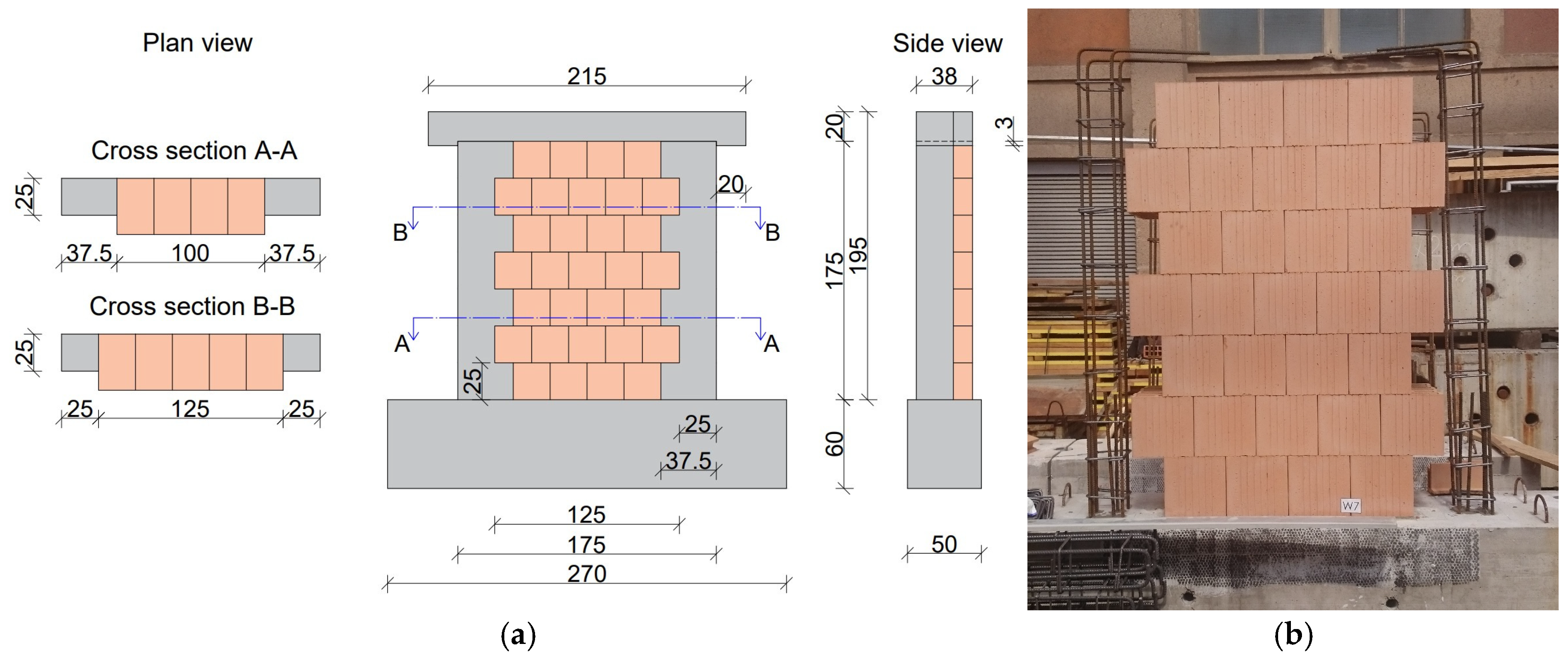
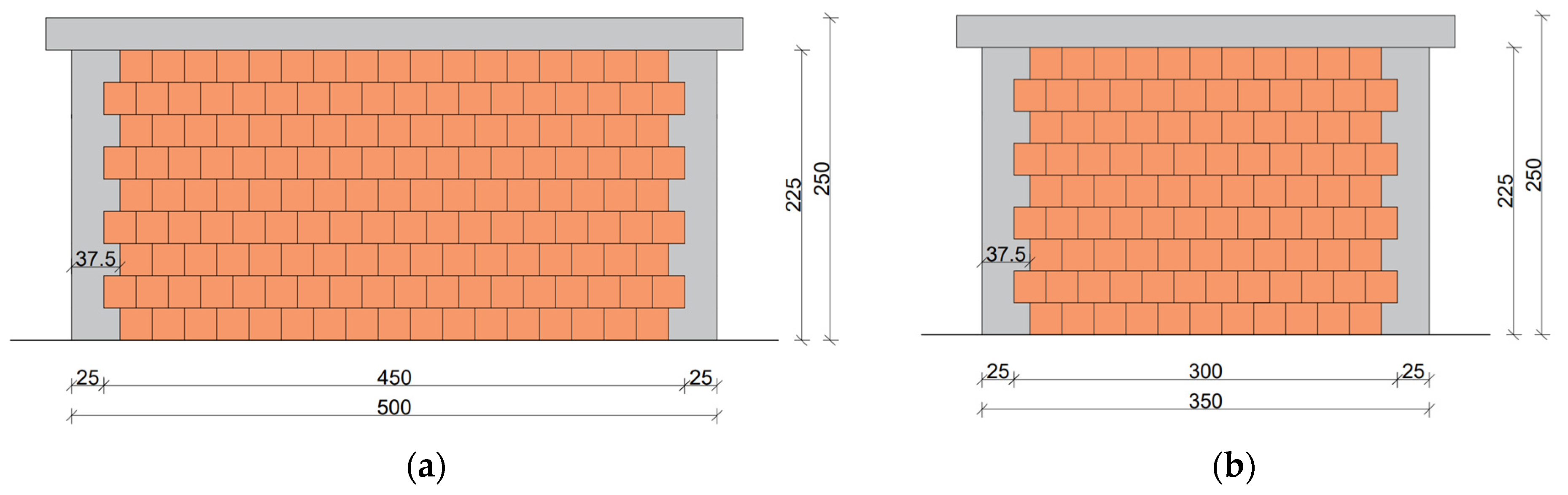
Two identical CM wall specimens, labelled W7 and W8, which were 175 cm long, 195 cm tall, and 38 cm thick (Figure 2a), were tested in the laboratory by Gams et al. [5]. The walls were built on an RC foundation beam to facilitate transport and fixation to the strong floor during the test. The tie-columns measured 25 × 25 cm (Figure 2a), and were reinforced with 4 Ø 14 mm ribbed bars, resulting in a longitudinal reinforcement ratio of 1%, as required by Eurocode 8 [3]. Transverse reinforcement consisted of Ø 8 mm stirrups spaced at about 20 cm (see Figure 2b). The tie-columns were flush with one side of the wall, while on the opposite side, they were depressed 13 cm from the surface, with the gap filled with thermal insulation. Finally, a spreader RC bond beam was cast together with the tie-columns.

The walls were tested under in-plane shear compression conditions at a constant vertical stress of 0.63 MPa. Rotations were prevented by using double-fixed boundary conditions. Horizontal displacements were cyclically applied at the level of the bond beam, with three repetitions per displacement amplitude in both directions, simulating seismic loading in a standard manner [28]. Detailed information regarding the test setup, instrumentation, loading protocol, and comprehensive test results can be found in the study by Gams et al. [5].

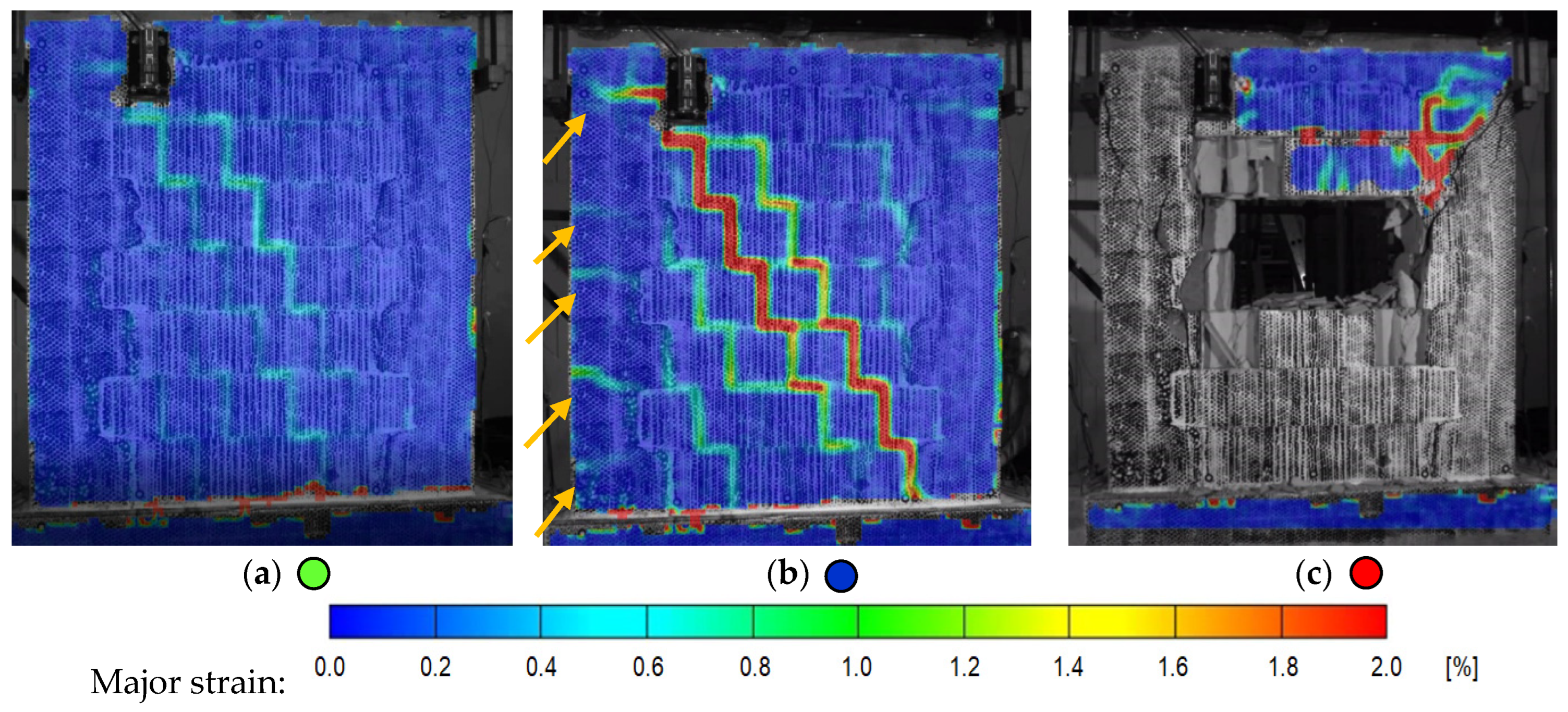
A digital image correlation (DIC) system was used to measure the displacement and strain fields on the wall surface. Figure 3 shows the damage progression at different limit states (LSs).

During the initial phase of testing, the CM walls showed linear behaviour up to a drift of around 0.1%. The first visible cracks appeared along the bed and head joints, gradually expanding as displacement amplitudes increased (Figure 3a). At approximately 0.35% drift, horizontal cracks developed in the tie-columns (marked with orange arrows in Figure 3b), and the protruding part of the masonry began to shear off. By 1.0% drift, damage in the left tie-column changed from evenly spread horizontal tensile cracks to concentrated shear damage at the upper corner of the wall. As the test progressed, the centre of the wall crumbled and disintegrated (Figure 3c), resulting in the near-collapse limit state. In the end, the tie-columns carried the entire vertical load, preventing the wall from losing its integrity.

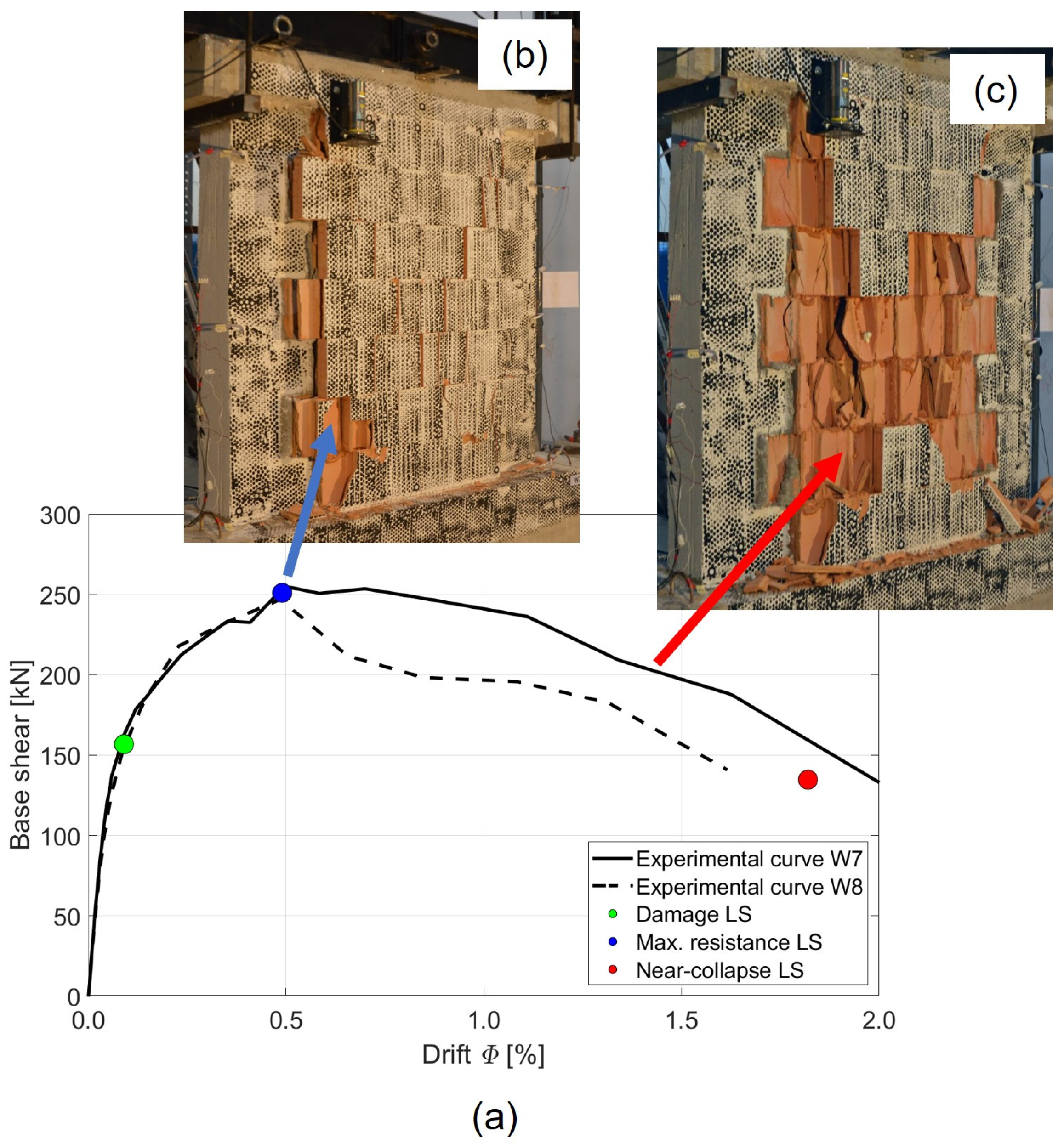
Averaged experimentally obtained envelope curves for both tested CM walls (in the push and pull directions) are presented in Figure 4a. LSs are denoted by differently coloured circles: green for damage LS, blue for maximum resistance LS, and red for near-collapse LS. At a drift of 0.5%, significant damage occurred, due to the shear-off effect at the interface between the tie-columns and the protruding masonry, causing pieces of masonry blocks to break off (Figure 4b). This damage contributed to reaching the maximum resistance LS. As shown in Figure 4c, the protruding masonry parts completely sheared off and fell to the floor at a drift of 1.3%.

3. Numerical Simulation and Modelling

This section provides a detailed description of the FE model used for the numerical simulations and validation of the in-plane seismic response of the tested CM walls. The FE model was developed using Abaqus/Explicit software [9], incorporating the actual geometry and material properties described in Section 2, to simulate both the global response and local damage of the CM walls. Initially, the model was validated against experimental results, before being used for parametric studies examining the influence of wall configuration and openings on the seismic response of CM walls.

3.1. The Numerical Model

The 3D FE model of the tested CM walls was built in Abaqus/Explicit [9], as shown in Figure 5. A fully 3D model was necessary to accurately capture and simulate the shear-off effect in the protruding masonry. The masonry units were modelled as solid elements without holes, and the effect of the holes was incorporated by modifying the material model for the masonry units according to Stavridis and Shing [30].

The geometry of the test specimen was fully modelled using the actual geometry and size of the specimen, except for the foundation, which was modelled by a discrete rigid plate in order to reduce computational effort and time. RC confining elements (tie-columns and tie-beam) and masonry units were modelled using 3D hexahedral continuum elements with eight nodes and reduced integration (C3D8R), in accordance with the recommendations for explicit dynamic analysis provided in [9]. Longitudinal bars and stirrups were represented using two-node wire 3D truss elements (T3D2), with their lengths and positions based on the tested specimens, as shown in Figure 5a. Interactions between the concrete and reinforcement bars were modelled using the “Embedded Constraint” feature in Abaqus, ensuring equality of displacements. The RC tie-columns were rigidly connected to the ground-fixed rigid plate through a “Tie Constraint”.

The boundary conditions in the numerical model were applied to match the experimental setup. The bottom surface (rigid plate in our model) was assumed to be fixed using the “Encastre” boundary condition (fixed BC), which effectively simulated the constraint provided by the foundation beam in the experiments.

The vertical loading in the FE model was aligned with the experimental setup, while the lateral in-plane loading was applied monotonically in the push direction, as opposed to the cyclic loading used in the experiments. Initially, gravity load was applied to the model, followed by vertical load on the wall and horizontal in-plane displacement at the bond beam level. The gravity load was defined as the total weight of the model, including the contributions from the concrete, masonry, and steel components, and it was applied prior to initiating the explicit dynamic analysis. Subsequently, the vertical pressure ${\sigma }_0=0.63 \mathrm{M}\mathrm{P}\mathrm{a}$ was applied as a uniformly distributed load over the upper surface of the bond beam, as shown in Figure 5b. Finally, an in-plane horizontal displacement was applied at the centre of the bond beam (Figure 5b). Additionally, geometric nonlinearities were assigned in all loading steps.

Several numerical simulations were conducted to determine the optimal loading time for each step, ensuring that dynamic effects were avoided. The duration of the first two steps was set to 1.0 s, while the main loading step lasted 12.5 s. In addition to selecting the appropriate loading time, the mesh size also needed to be determined. Through a process of gradual refinement, the optimal mesh size of 32.5 mm was identified (almost four elements along the protruding part of masonry). The mesh of the FE model with solid units is shown in Figure 6.

3.2. Contact and Interface Definitions

The interface properties between masonry units, and between masonry units and RC elements, were defined using the general contact available in Abaqus [9], with specified interaction properties to accurately simulate the interface behaviour. To achieve this, three distinct interaction properties were established, as illustrated in Figure 7. To model the interaction between the masonry units and the RC tie-elements, a “Tie” constraint was applied to simulate the chemical bond formed during the concreting. This constraint created a rigid connection at all wall-to-tie-element interfaces, except for the top surface of the RC foundation beam, which was modelled as a rigid plate in our case, where the masonry blocks were laid. The rigid connection is depicted by the black dashed line in Figure 7. For the global interaction properties, “hard” contact was applied in the normal direction to prevent surface penetration (i.e., the slave surface into the master surface) and to ensure that no tensile stresses were transferred across the interfaces.

For the global interaction properties, “hard” contact was applied in the normal direction to prevent surface penetration (i.e., slave surface into master surface), and to ensure that there were no transferred tensile stresses across the surfaces. In the tangential direction, a penalty friction formulation was used, with a friction coefficient derived from experimental tests. This allowed only compressive stresses and frictional forces to be transferred when the surfaces were in contact. Since the head joints were unfilled, global interaction properties were applied to these interfaces (shown as a red solid line in Figure 7). For other specific interactions, such as those between horizontal surfaces in contact, individual contact properties were defined to override the global properties. This method ensured an accurate representation of the bed-joint behaviour and the complex interactions between the masonry units.

The behaviour of the bed-joints was defined using individual contact properties, which incorporated a surface-based cohesive interaction in conjunction with the previously established global interaction properties, including “hard” contact and penalty friction assignment. This cohesive interaction, represented by the blue solid line in Figure 7, was employed to model the horizontal contact surfaces between masonry blocks bonded with PU glue. The use of surface-based cohesive interaction is particularly relevant when the interface thickness is negligibly small, such as in cases where PU glue is used instead of traditional mortar. Due to the negligible thickness of the PU-filled joints, the interaction was defined directly between the individual masonry units.

Initially, the contact behaviour is assumed to be linear elastic, with uncoupled stiffness in all three directions, characterized by normal stiffness ($K_{nn}$) and shear stiffness values ($K_{ss} \mathrm{a}\mathrm{n}\mathrm{d} K_{tt}$). As long as the maximum tensile or shear stresses are not exceeded, the interaction remains linear in shear. However, once these maximum stresses are reached, degradation begins, eventually leading to the failure of the contact. These elastic stiffnesses are calculated according to the following equations, proposed by Nazir and Dhanasekar [31]:

$$K_{nn}={\displaystyle \frac{E_u{E}_m}{E_u\left(h_u+t_j\right)-E_m{h}_u}}$$

(1)

$$K_{ss}=K_{tt}={\displaystyle \frac{K_{nn}}{2\left(1+\nu \right)}}$$

(2)

where $E_u$ and $h_u$ are the elastic modulus and height of the unit, respectively; $E_m$ is the modulus of elasticity of masonry; and $t_j$ is the thickness of the PU-filled joint, which is taken as 1 mm for the calculation. The modulus of elasticity of the unit, $E_u$, is assumed to be $300·f_b$, as suggested by Kaushik et al. [32].

The damage initiation criterion in the contact is based on the quadratic traction law. The maximum tensile stress (denoted as $t_n$) was taken from the literature [33] and assumed as the threshold for damage initiation in the contact surface. In parallel, the maximum shear stresses, denoted as $t_s$ and $t_t$, were derived from triplet tests on masonry samples, which were tested both with and without precompression (see Section 2 in [5] for more details). Upon reaching the damage initiation threshold, the model used a damage evolution law to describe how the cohesive stiffness degrades. To model the damage evolution in a proper way, fracture energies in the normal direction for Mode I ($G_n)$ and in the two shear directions for Mode II ($G_s$ and $G_t$) were defined through a calibration process and values available in the relevant literature [13]. The chosen damage evolution model was an energy-based exponential mixed-mode law, with a cohesive parameter, η, taken from a prior study [33].

During the final calibration of the FE model, the stiffness values $K_{nn}$, $K_{ss}$, and $K_{tt}$ were adjusted by reducing them by 20% to improve agreement with the experimental results. An overview of all the values used for defining the interaction properties is presented in

Table 1. Overview of property values used for definition of interaction.

Properties	Symbol	Value	References
Elastic stiffness in the normal direction	$K_{nn}$	23.13 MPa/mm	Calculated
Elastic stiffness in the shear direction	$K_{ss}$$, K_{tt}$	9.64 MPa/mm	Calculated
Maximum tensile stress	$t_n$	0.12 MPa	The literature [33]
Maximum shear stress	$t_s$$, t_t$	0.097 MPa	Dedicated tests
Fracture energy Mode I	$G_n$	0.001 N/mm	Calibrated
Fracture energy Mode II	$G_s$$, G_t$	0.5 N/mm	The literature [13]
Cohesive parameter	η	2.0	The literature [33]
Friction coefficient	$tan \alpha$	0.57	Dedicated tests

.

3.3. Material Model Definition

The Concrete Damaged Plasticity (CDP) model, one of the most well-known material models in Abaqus [9], was adopted to simulate the inelastic behaviour of both concrete and masonry units, as it effectively captures the response of quasi-brittle materials, such as masonry, under both monotonic and cyclic loading. The model uses a yield function originally introduced by Lubliner et al. [34], with refinements by Lee and Fenves [35] to account for differences in strength evolution under tension and compression. The CDP model is based on a non-associated flow rule, with material dilatancy controlled through a parameter known as the dilation angle. In this study, a dilation angle of 36° for concrete and 30° for masonry units was initially adopted, which is consistent with recommendations in the literature [33,36]. Other key parameters used to define the shape of the yield function included the flow potential eccentricity ($\epsilon =0.1$), the ratio of equibiaxial compressive yield stress to uniaxial compressive yield stress (${\sigma }_{b0}/{\sigma }_{c0}=1.16$), and the ratio of the second stress invariant on the tensile meridian to that on the compressive meridian at initial yield ($K=2/3$), all of which were based on default values provided by Abaqus. To further enhance model stability and ensure an accurate simulation of the material’s inelastic behaviour, the viscosity parameter was set to zero.

3.3.1. Concrete and Steel Reinforcement

The elastic behaviour of concrete is assumed to be linear and isotropic, characterized by Young’s modulus and a Poisson’s ratio of 0.2. The modulus of elasticity for concrete class C 30/37 is taken from Eurocode 2 [37]. To fully capture the plastic response of concrete, separate stress–strain (for compression) and stress–displacement (for tension) curves are required. The properties used to define the material model for concrete, and subsequently applied in the numerical model, are presented in

Table 2. Properties of material model for concrete used in FE model.

Properties	Symbol	Value	References
Modulus of elasticity	$E_{cm}$	33,000 MPa	Eurocode 2 [37]
Compressive strain at end of elastic part of stress–strain curve (point B, Figure 8a)	${\epsilon }_{c,\mathrm{e}\mathrm{l}}$	0.0461%	Calculated
$\mathrm{Compressive} \mathrm{strength} \mathrm{corresponding} \mathrm{to} \mathrm{strain} {\epsilon }_{c,\mathrm{e}\mathrm{l}}$$, \mathrm{equal} \mathrm{to} 0.4 f_{cm}$	$f_{c,\mathrm{e}\mathrm{l}}$	15.12 MPa	Calculated
$\mathrm{Compressive} \mathrm{strain} \mathrm{at} \mathrm{peak} \mathrm{stress} f_{cm}$(point C, Figure 8a)	${\epsilon }_{c,1}$	0.22%	Eurocode 2 [37]
Mean value of concrete cylinder compressive strength at 28 days	$f_{cm}$	38.0 MPa	Eurocode 2 [37]
Compressive strain at point D of sinusoidal descending part of stress–strain curve (upper point, Figure 8a)	${{\epsilon }_{c,u1}=\epsilon }_{c,uD}$	0.35%	Eurocode 2 [37]
$\mathrm{Compressive} \mathrm{strength} \mathrm{corresponding} \mathrm{to} \mathrm{nominal} \mathrm{ultimate} \mathrm{compressive} \mathrm{strain} {\epsilon }_{c,u1}$$={\epsilon }_{c,uD}$	$f_{c,uD}$	24.86 MPa	Calculated
Compressive strain at point E of sinusoidal descending part of stress–strain curve (lower point, Figure 8a)	${\epsilon }_{c,uE}$	3.0%	Literature [36]
$\mathrm{Compressive} \mathrm{strength} \mathrm{corresponding} \mathrm{to} \mathrm{compressive} \mathrm{strain} \mathrm{at} \mathrm{failure} {\epsilon }_{c,uE}$	$f_{c,uE}$	2.0 MPa	Calculated
$\mathrm{Ratio} \mathrm{between} f_{cm}$$\mathrm{and} f_{c,uE}$	${\alpha }_{red}$	19.0	Calibrated
Tangent factor at point D	${\alpha }_{tD}$	0.5	Literature [36]
Tangent factor at point E	${\alpha }_{tE}$	0.9	Literature [36]
$\mathrm{Ratio} \mathrm{between} f_{cm}$$\mathrm{and} f_{c,uD}$	$\beta$	1.529	Calculated
Compression damage evolution parameter	$a_C$	150.0	Calibrated
Mean value of axial tensile strength at 28 days (point B, Figure 8b)	$f_{\mathrm{c}\mathrm{t}\mathrm{m}}$	2.9 MPa	Eurocode 2 [37]
Strain at maximum tensile strength	${\epsilon }_{cr}$	0.0088%	Calculated
First material constant	$c_1$	3.0	Literature [38]
Second material constant	$c_2$	6.93	Literature [38]
Fracture energy of concrete	$G_F$	182.65 N/m	Calculated
Critical crack opening (point C, Figure 8b)	$w_c$	0.324 mm	Calculated
Tension damage evolution parameter	$a_t$	225.0	Calibrated
Length of finite element	$l_{\mathrm{e}\mathrm{q}}$	32.5 mm	Calibrated

, where it is indicated which values were taken directly from the relevant standard, calculated based on recommendations in the literature, or calibrated.

The stress–strain curve under compression follows a linear behaviour up to 0.4 $f_{cm}$ (from point A to point B, as shown in Figure 8). Beyond this point, from point B to point D (Figure 8), concrete enters the plastic region, and the stress–strain behaviour is defined by the expression provided in Eurocode 2 [37]:

$${\displaystyle \frac{{\sigma }_c}{f_{cm}}}={\displaystyle \frac{k\eta -{\eta }^2}{1+\left(k-2\right)\eta }}$$

(3)

where $\eta ={\epsilon }_c/{\epsilon }_{c,1}$ and $k=1.05 {\epsilon }_{c,1}{E}_{cm}/f_{cm}$ are calculated according to Eurocode 2 [37]. The strain ${\epsilon }_{c,1}$ corresponds to the strain at the peak stress $f_{cm}$, which is represented by point C in Figure 8a. The ultimate strain ${\epsilon }_{c,u1}$ (${\epsilon }_{c,uD}$) was equal to 0.35% (point D; Figure 8a), while the corresponding compressive stress at point D, $f_{c,uD}={\sigma }_c\left({\epsilon }_{c,uD}\right)$, was calculated using Equation (3). To model the concrete response beyond a strain of 3.5 ‰, the curve was extended from point D to point E (Figure 8a) using a sinusoidal function, as proposed by Pavlović [36]:

$${\sigma }_c\left({\epsilon }_c\right)=f_{cm}\left[{\displaystyle \frac{1}{\beta }}-{\displaystyle \frac{\sin \left({\mu }^{{\alpha }_{tD}}·{\alpha }_{tE}\frac{\pi }{2}\right)}{\beta ·\sin \left({\alpha }_{tE}\frac{\pi }{2}\right)}}+{\displaystyle \frac{\mu }{{\alpha }_{red}}}\right]$$

(4)

where ${\alpha }_{red}$ represents the ratio between $f_{cm}$ and $f_{c,uE}$, $\beta$ denotes the ratio between $f_{cm}$ and $f_{c,uD}$, factors ${\alpha }_{tD}$ and ${\alpha }_{tE}$ control the tangent angles of the sinusoidal part beyond point D (values provided in Table 2), and $\mu$ represents the relative coordinate between points D and E, calculated as follows:

$$\mu ={\displaystyle \frac{\left({\epsilon }_c-{\epsilon }_{c,uD}\right)}{\left({\epsilon }_{c,uE}-{\epsilon }_{c,uD}\right)}}$$

(5)

Point E is the end point of the sinusoidal part of the curve, with a strain ${\epsilon }_{c,uE}$ and a stress $f_{c,uE}$ which is reduced by a factor ${\alpha }_{red}$, as shown in Figure 8a.

The behaviour of concrete under tension is described using a fracture energy criterion, which defines the relationship between crack width $w_c$ and tensile stress ${\sigma }_t$, as proposed by Hordijk [38]:

$${\displaystyle \frac{{\sigma }_t\left(w\right)}{f_{ctm}}}=\left[1+{\left(c_1{\displaystyle \frac{w}{w_c}}\right)}^3\right]e^{{-c}_2{\displaystyle \frac{w}{w_c}}}-{\displaystyle \frac{w}{w_c}}(1+c_1^3)e^{{-c}_2}$$

(6)

where $f_{ctm}$ denotes the maximum tensile strength according to Eurocode 2 [37]; $w_c$ is the critical crack opening; and parameters $c_1$ and $c_2$ represent material constants used to fit the curve, as stated in [38].

The deformation in the softening branch of the tensile behaviour includes both strain and crack displacement (crack opening). To account for the material’s strain-softening behaviour, Hordijk [38] proposes a separation of the stress–deformation diagram into two components: one capturing the stress–strain behaviour of the bulk material, and the other addressing the stress–displacement relationship caused by crack propagation. The stress–crack opening curve depends on the fracture energy $G_F$, which indicates the area under the stress–displacement curve (Figure 8b).

The critical crack width $w_c$ is further linked to fracture energy by the following expression:

$$w_c=5.14{\displaystyle \frac{G_F}{f_{ctm}}}$$

(7)

In the absence of experimental data, $G_F$ can be estimated using the equation from CEB-FIP Model Code 2010 [39]:

$$0.7·73f_{cm}^{0.18}\le G_F\le 1.3·73f_{cm}^{0.18}$$

(8)

In this study, $G_F$ was taken as an upper boundary of the range given in Equation (8). The values for $G_F$ and $w_c$ are provided in Table 2.

To accurately describe the tensile behaviour of concrete beyond its maximum strength $f_{ctm}$, the corresponding strain was calculated using the equation given in a study by Lopez Almansa et al. [40]:

$${\epsilon }_t={\epsilon }_{\mathrm{c}\mathrm{r}}+{\displaystyle \frac{u_{\mathrm{c}\mathrm{r}}}{l_{\mathrm{e}\mathrm{q}}}}$$

(9)

where ${\epsilon }_{cr}$ is the strain at the maximum tensile strength, $u_{\mathrm{c}\mathrm{r}}$ represents the crack opening, and $l_{eq}$ is the length of the finite element, which is determined as part of the sensitivity study discussed earlier in this Section.

The stress–strain relationship under compression and the stress–displacement curves for the concrete material are shown in Figure 8.

Since the CDP model for reinforced concrete (RC) treats the behaviour of concrete and steel reinforcement separately, the interaction effects between the rebar and concrete, such as bond effect or dowel action, are considered by introducing the concept of “tension stiffening”, which is incorporated into the model by defining the concrete material by a stress–displacement curve, which accurately captures the material’s response under tensile loading.

The behaviour of the steel reinforcement was represented using a bilinear model, derived from test results on the rebars (see Section 2 in [5] for more details). This model assumes an elasto-plastic material with isotropic hardening, effectively capturing the transition from elastic to plastic deformation under loading. The following material properties are employed: modulus of elasticity $E_s=200 \mathrm{G}\mathrm{P}\mathrm{a}$, Poisson’s ratio ${\nu }_s=0.3$, yield stress $f_y=551 \mathrm{M}\mathrm{P}\mathrm{a}$, ultimate stress $f_u=658 \mathrm{M}\mathrm{P}\mathrm{a}$, and ultimate strain ${\epsilon }_u=10\%$.

3.3.2. Masonry Units

The material model for masonry was defined by adjusting the modulus of elasticity and compressive strength of the solid blocks, as used in this study, instead of the hollow blocks, following the recommendations of Stavridis and Shing [30]. The stress–strain relationship for masonry under compression was defined as linear up to point B (Figure 9a), with the modulus of elasticity $E_m$ and a Poisson’s ratio of 0.2. Beyond the elastic region, the nonlinear portion of the stress–strain curve up to point D (Figure 9a) was also modelled using their approach, as follows:

$$\sigma =f_{c,m}\left(2{\displaystyle \frac{\epsilon }{{\epsilon }_1}}-{\displaystyle \frac{{\epsilon }^2}{{\epsilon }_1^2}}\right)$$

(10)

where ${\epsilon }_1$ presents the strain at maximum compressive strength $f_{\mathrm{c},\mathrm{m}}$ (point C; Figure 9a), obtained through calibration process. The behaviour of masonry beyond point D, where the stress drops to 90% of $f_{\mathrm{c},\mathrm{m}}$, was defined based on the modified equation proposed by Marinković and Butenweg [33]:

$$\sigma ={\sigma }_D+\left\{\left[\sin \left(1-e^{\left[{\displaystyle \frac{f_{c,m}}{E·\epsilon }}\left({\displaystyle \frac{\epsilon }{{\epsilon }_1}}-{\displaystyle \frac{{\epsilon }_D}{{\epsilon }_1}}\right)\right]}\right)\right]\pi ·\alpha \right\}$$

(11)

where ${\sigma }_D$ and ${\epsilon }_D$ represent the stress and strain at point D (Figure 9a). These material parameters, along with the residual strength of the masonry (assumed to be 20% of $f_{c,m}$), were calibrated to ensure the best match with the experimentally obtained force–displacement curve. A reduction factor $\alpha$ of 3.4 was obtained to reach this level for residual masonry compressive strength.

The tensile behaviour of masonry was described using the equation suggested by Stavridis and Shing [30]:

$${\sigma }_t=f_{t,m}\left[r_t+\left(1-r_t\right)e^{\left({\displaystyle \frac{-{\alpha }_1\left(\epsilon -{\epsilon }_{m,cr}\right)}{f_{t,m}}}\right)}\right]$$

(12)

where ${\epsilon }_{m,cr}$ is the strain corresponding to the maximum tensile strength $f_{t,m}$ (assumed to be 11% of $f_{c,m}$). The slope of the stress–strain curve was defined by the parameters ${\alpha }_1$ and $r_t$, both of which were calibrated to ensure a close fit with the experimental results (see

Table 3. Properties of material model for masonry units used in FE model.

Properties	Symbol	Value	References
Modulus of elasticity	$E_m$	2200 MPa	Dedicated tests
Compressive strain at end of elastic part of stress–strain curve (point B, Figure 9a)	${\epsilon }_{m,el}$	0.015%	Calibrated
$\mathrm{Compressive} \mathrm{strength} \mathrm{corresponding} \mathrm{to} \mathrm{strain} {\epsilon }_{c,\mathrm{e}\mathrm{l}}$	$f_{c,m,el}$	0.32 MPa	Calibrated
$\mathrm{Compressive} \mathrm{strain} \mathrm{at} \mathrm{peak} \mathrm{strength} f_m^{\mathrm{’}}$ (point C, Figure 9a)	${\epsilon }_1$	0.4%	Calibrated
Compressive strength of masonry	$f_{c,m}$	3.79 MPa	Dedicated tests
Compressive strain at point D (Figure 9a)	${\epsilon }_D$	0.53%	Calibrated
$\mathrm{Compressive} \mathrm{strength} \mathrm{corresponding} \mathrm{to} 0.9 \mathrm{of} f_m^{\mathrm{’}}$	${\sigma }_D=0.9f_{c,m}$	3.41 MPa	Calculated
Residual strength reduction factor	$\alpha$	3.4	Calibrated
Compression damage evolution parameter	$a_C$	155.0	Calibrated
Tensile strength of masonry (point B, Figure 9b)	$f_{t,m}$	0.417 MPa	Calculated
Strain at maximum tensile strength	${\epsilon }_{m,\mathrm{c}\mathrm{r}}$	0.019%	Calculated
Residual tensile strength of masonry (point C, Figure 9b)	$f_{t,m,res}$	0.022 MPa	Calculated
$\mathrm{Ratio} \mathrm{of} \mathrm{residual} f_{t,m,res}$$\mathrm{to} \mathrm{peak} \mathrm{tensile} \mathrm{strength} f_{t,m}$	$r_t$	0.05	Calibrated
Initial slope factor	${\alpha }_1$	250.0	Calibrated
Tension damage evolution parameter	$a_t$	312.5	Calibrated

). Specifically, $r_t$ represents the ratio of the residual tensile strength to the maximum tensile strength, effectively controlling the tail of the stress–strain curve and its transition to nearly zero stress.

To characterize the behaviour beyond the maximum tensile strength $f_{t,m}$, the corresponding strain was determined according to the same approach as taken by Lopez-Almansa et al. [40], which was applied for the material model of concrete (see Equation (9)). The stress–crack opening curve is presented in Figure 9b.

The material properties used to define the material model for the masonry units are summarized in Table 3, which also specifies whether the values were sourced from dedicated tests, calculated, or obtained through calibration.

3.3.3. Damage Model for Concrete and Masonry Units

To fully define the behaviour of concrete and masonry under both compression and tension, the degradation of elastic stiffness must be considered. This is accomplished by introducing two damage variables, $d_c$ and $d_t$, which govern the material’s stiffness reduction under compression and tension, respectively. These damage variables are defined as functions of the inelastic strain ${\epsilon }_c^{\mathrm{i}\mathrm{n}}$ (for compression) and cracking strain ${\epsilon }_t^{\mathrm{c}\mathrm{k}}$ (for tension). The range of these parameters is from 0 to 1, describing the transition from undamaged to completely damaged material [9]. The damage evolution is represented using the exponential Equations (13) and (14), as proposed by Lee and Fenves [35]:

$$d_c=1-e^{-a_c{\epsilon }_c^{\mathrm{i}\mathrm{n}}}$$

(13)

$$d_t=1-e^{-a_t{\epsilon }_t^{\mathrm{c}\mathrm{k}}}$$

(14)

The damage evolution parameters $a_c$ and $a_t$ for concrete material are provided in Table 2, while the corresponding values for masonry are reported in Table 3. These parameters were obtained through a calibration process to ensure a better match with the experimental results. The damage evolution curves for concrete and masonry are presented in Figure 10 and Figure 11, respectively.

3.4. Validation of Numerical Model

The validation of the numerical model was performed by comparing the results of the simulation with the experimental results from the two test specimens. The primary comparison focuses on the global response of the CM wall specimens, specifically the hysteretic response envelopes (averaged over both push and pull directions) and the force–drift curve, represented by the blue curve, which was obtained from the numerical model in Abaqus/Explicit (Figure 12). The numerical result closely matched the experimental results, especially regarding the initial stiffness. The peak capacity predicted by the model was also well aligned with the experimental results, with only minor discrepancies of 7.4% for specimen W7 and 4.4% for specimen W8. Furthermore, the drift at which peak capacity occurred was nearly identical, with the numerical model predicting a drift of 0.44%, compared to approximately 0.5% observed in the experiments. Overall, the numerical model’s response after reaching peak capacity was consistent with the average response of both specimens. The damage evolution was also quite accurately predicted, as is presented in detail in a study by Krtinić et al. [41].

4. Parametric Study

The aim of the parametric study was to investigate the effect of aspect ratio (AR), opening configurations, and RC tie-columns on the seismic performance. A total of 20 different models were analyzed, with different opening sizes, shapes, and positions, and different tie-column positions and sizes. An overview of the models is shown in

Table 4. Overview of parametric study.

Model No.	Model Name	Aspect Ratio	Opening Shape/ Position	Opening Size	Internal Tie-Column Size
1	SW_1	0.5	Solid wall	-	-
2	SW_2	0.71	Solid wall	-	-
3	CWop_1	0.5	Central window	1.0 × 1.25 m2	-
4	CWop_2	0.71	Central window	0.75 × 1.0 m2	-
5	CWopEC_1	0.5	Central window	1.25 × 1.25 m2	-
6	CWopEC_2	0.71	Central window	1.25 × 1.25 m2	-
7	CDop_1	0.5	Central door	1.0 × 2.25 m2	-
8	CDop_2	0.71	Central door	1.0 × 2.25 m2	-
9	LWop_1	0.5	Left window	1.0 × 1.25 m2	-
10	LWop_2	0.71	Left window	0.75 × 1.0 m2	-
11	RWop_1	0.5	Right window	1.0 × 1.25 m2	-
12	RWop_2	0.71	Right window	0.75 × 1.0 m2	-
13	CWopEC_1-conA	0.5	Central window	1.25 × 1.25 m2	25 × 25 cm
14	CWopEC_2-conA	0.71	Central window	1.25 × 1.25 m2	25 × 25 cm
15	CDop_1-conA	0.5	Central door	1.0 × 2.25 m2	25 × 25 cm
16	CDop_2-conA	0.71	Central door	1.0 × 2.25 m2	25 × 25 cm
17	CWopEC_1-conB	0.5	Central window	1.25 × 1.25 m2	15 × 15 cm
18	CWopEC_2-conB	0.71	Central window	1.25 × 1.25 m2	15 × 15 cm
19	CDop_1-conB	0.5	Central door	1.0 × 2.25 m2	15 × 15 cm
20	CDop_2-conB	0.71	Central door	1.0 × 2.25 m2	15 × 15 cm

, where each model is identified by its name, representing a different combination of aspect ratio and opening shape/position, as well as the presence of tie-columns around openings and, if applicable, their size. In the naming, SW stands for solid wall, C/L/R indicates the position of the opening (central/left/right), ‘Wop/Dop’ stand for window or door opening, 1 or 2 are aspect ratios (1 stands for AR = 0.5 and 2 for AR = 0.71), and EC indicates a window opening larger than 1.5 m². ConA and conB designate the size of the internal tie-columns next to the openings. In the case of conA, the size is 25 × 25 cm, and in the case of conB, the size is 15 × 15 cm. All the walls have 25 × 25 cm tie-columns at the sides (see Figure 13).

Two different ARs were considered ($H_w/L_w=0.5$ and $H_w/L_w=0.71$), with the CM wall height fixed at 2.5 m and CM wall lengths of 5 m and 3.5 m, ensuring compliance with the Eurocode 8 [3] requirement that the maximum horizontal spacing between vertical confining elements should not exceed 5 m. These geometry configurations ensured that the numerical models represented real CM walls, reflecting the typical dimensions and proportions found in CM structures.

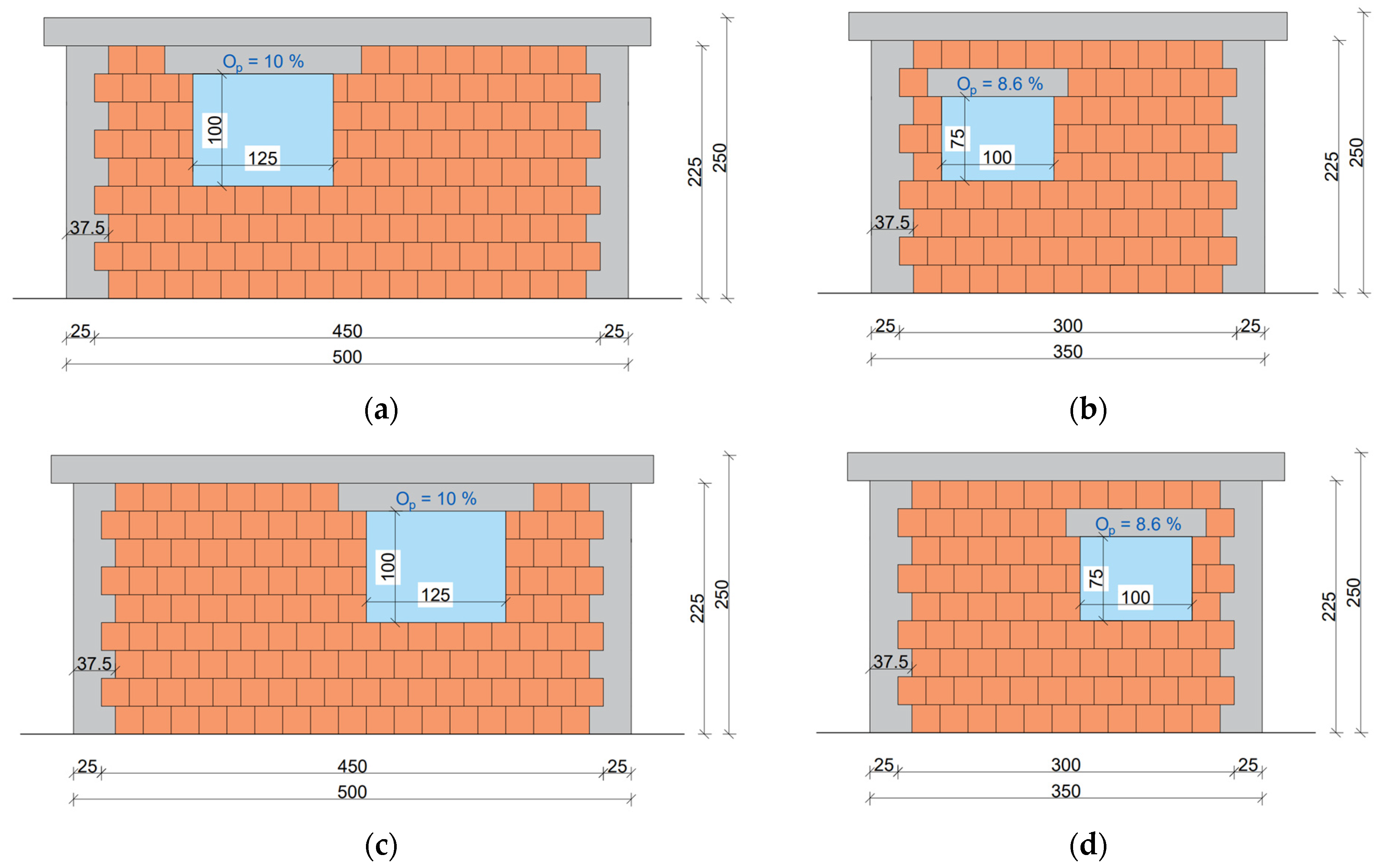
For AR = 0.5, the window dimensions were 1.0 × 1.25 m, and for AR = 0.71, they were 1.0 × 0.75 m. The opening percentages ($O_p$s) were 10% and 8.6%, respectively. Because both of these windows are small enough, codes and guidelines do not require tie-columns to be built next to them. The limit for this is 10% of the wall area according to Brzev and Mitra [19] and Meli et al. [17], and 1.5 m² according to Eurocode 8 [3]. The windows were considered in central, left, and right positions.

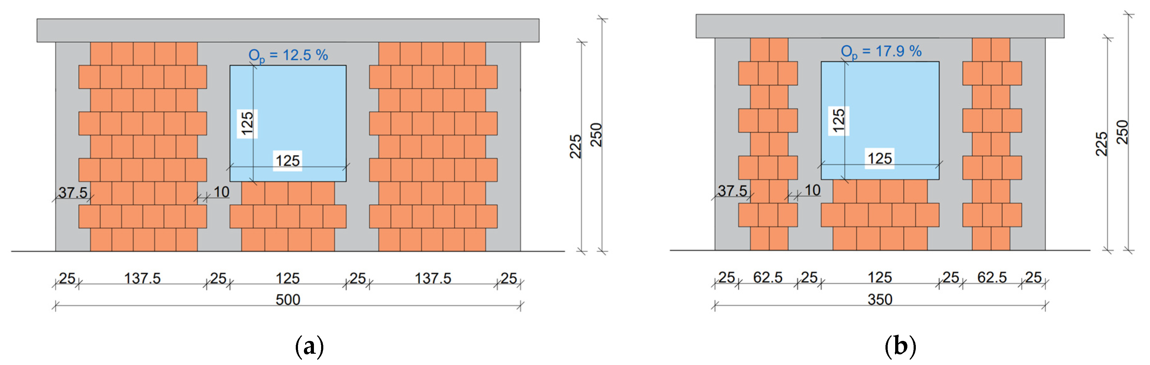
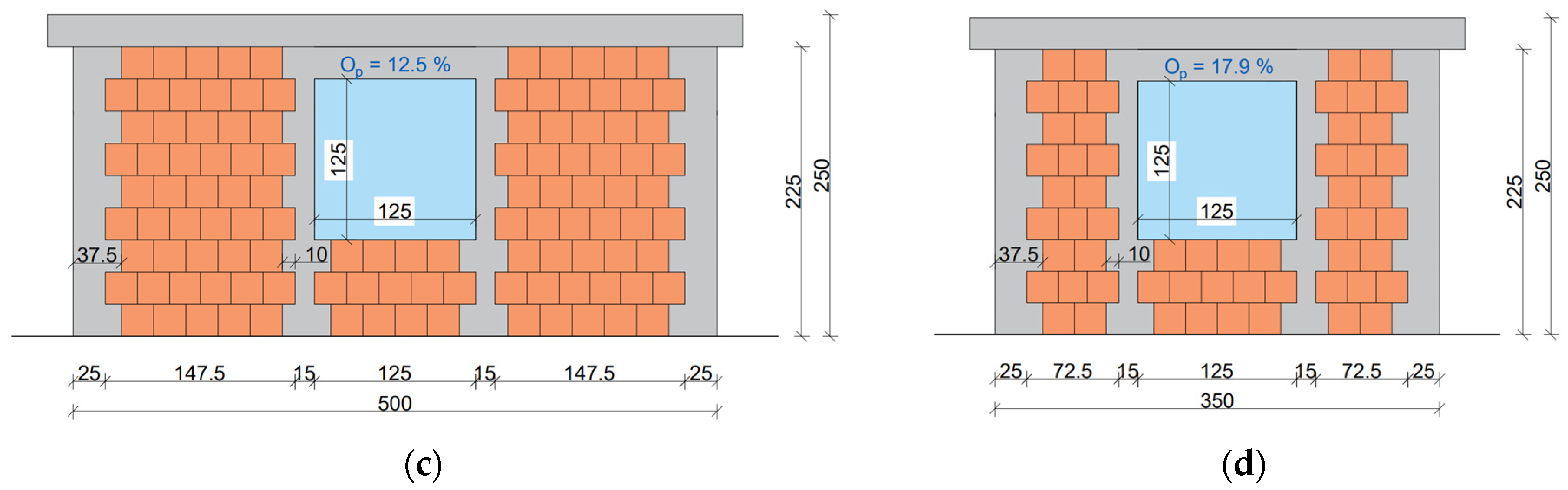
To analyze a case with a large enough window to require tie-columns, one case per AR was considered, with a window sized 1.25 × 1.25 m (area of 1.56 m²). In this case, the opening percentages ($O_p$) were 12.5% and 17.9% for walls with ARs of 0.5 and 0.71, respectively. This window was considered only in the central position, and with 15 × 15 cm and 25 × 25 cm tie-columns.

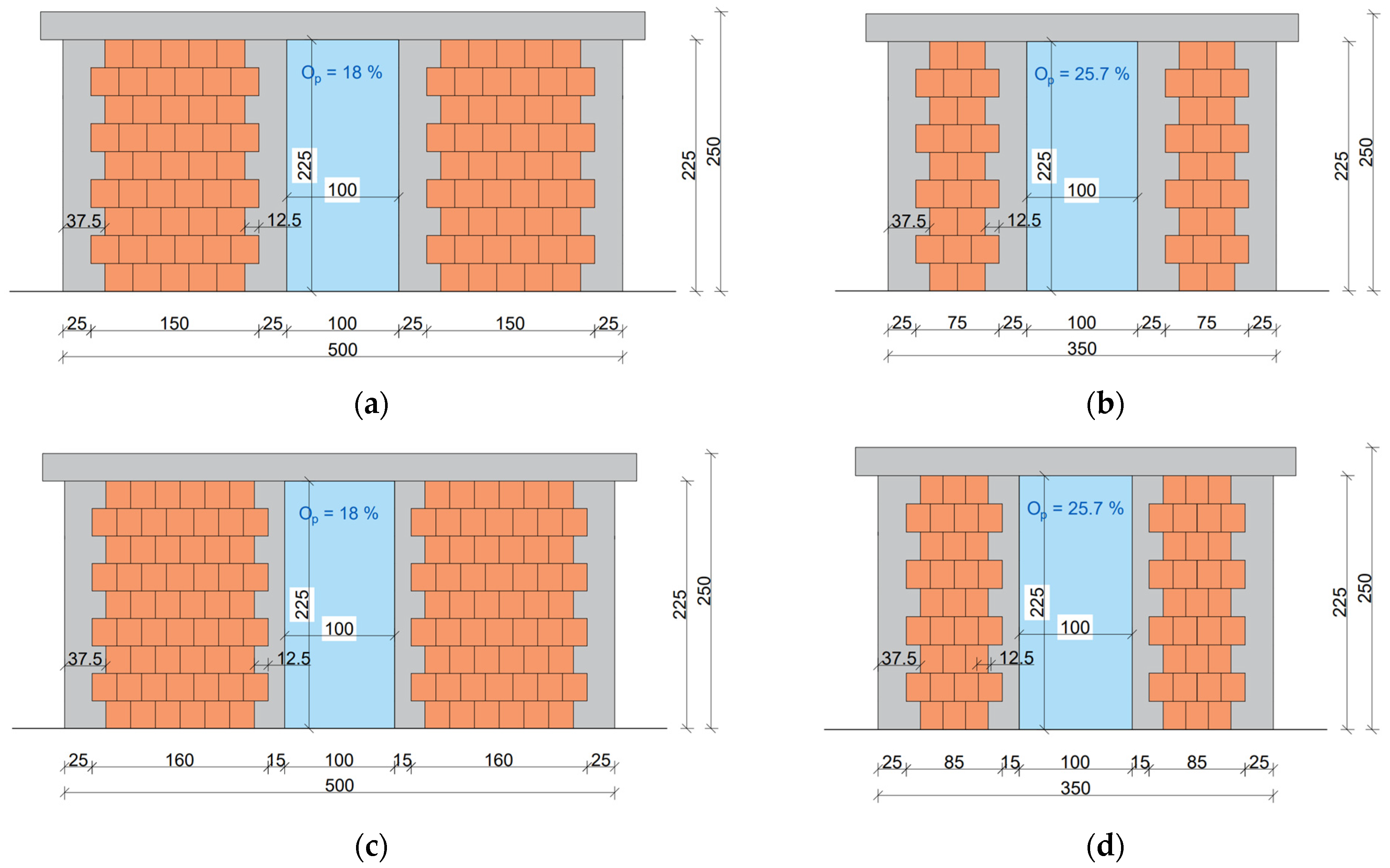
The door opening dimensions were 1.0 × 2.25 m, resulting in $O_p$s of 18% and 25.7% for walls with AR = 0.5 and AR = 0.71, respectively. The doors, too, were considered only in the central position, and with either 15 × 15 cm or 25 × 25 cm tie-columns.

4.1. Effect of Opening Size and Position on Seismic Response of CM Walls

4.1.1. Effect of Opening Size

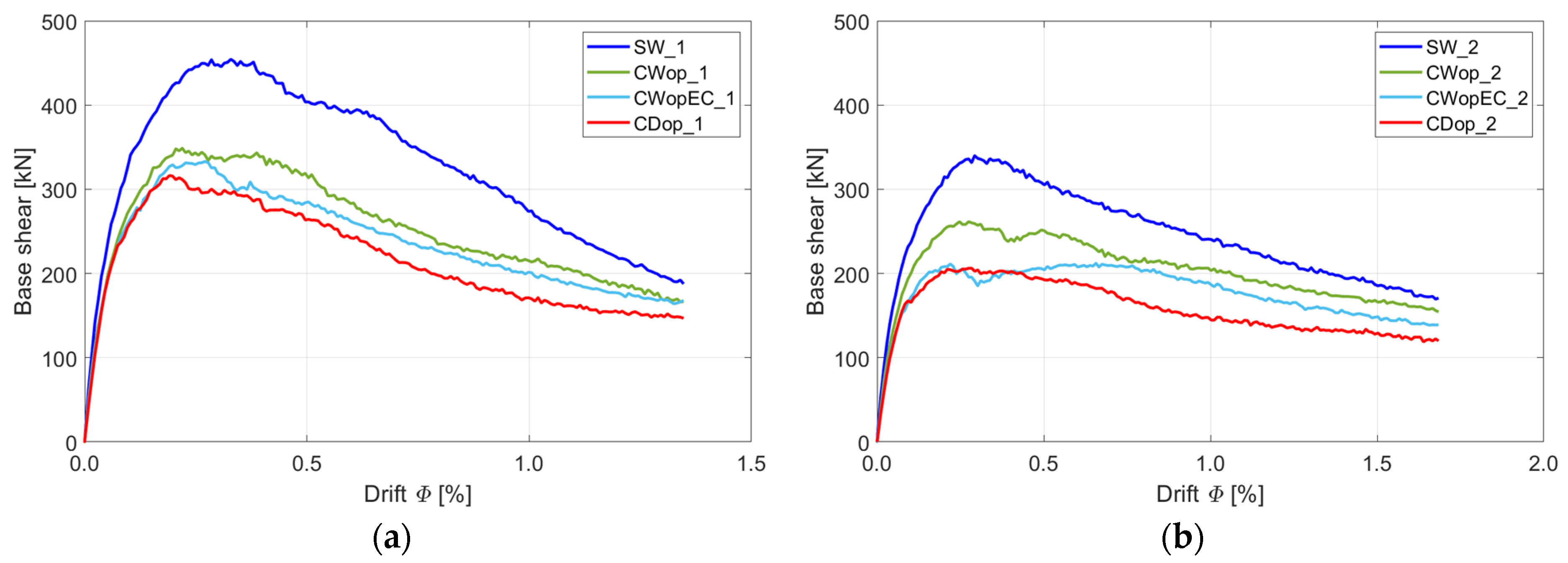
To examine the influence of opening size on the seismic response of CM walls, walls with a central position of the opening and no internal tie-columns were compared with the reference solid walls (shown in Figure 13). The pushover curves for the analyzed CM walls with varying opening sizes (window or door type) are shown in Figure 14. It is evident that the presence of openings significantly reduces the strength of the walls compared to the solid ones (SW1, SW2). For example, comparing the solid wall SW_1 with the wall containing a 10% opening (CWop_1), the reduction in strength is 23%. Similarly, for walls with AR = 0.71, the wall CWop_2, which has an opening of 8.6%, exhibits the same 23% reduction in strength compared to the solid wall SW_2. When comparing walls with larger openings, the strength loss becomes even more pronounced. For walls with AR = 0.5, there is an increase in opening size from 10% (CWop_1) to 12.5% (CWopEC_1), leading to a strength reduction of 27% compared to the solid wall SW_1. On the other hand, for walls with AR = 0.71, the effect of larger openings is more severe. For instance, increasing the opening size from 8.6% to 17.9% (CWopEC_2) results in a 38% strength loss compared to the solid wall SW2.

These findings highlight a clear relationship between the size of the openings, the aspect ratio (AR), and the reduction in wall strength. As the opening size increases, the strength reduction becomes more significant, with walls having AR = 0.71 experiencing a more substantial loss in load-bearing capacity, due to the amplified effect of larger openings.

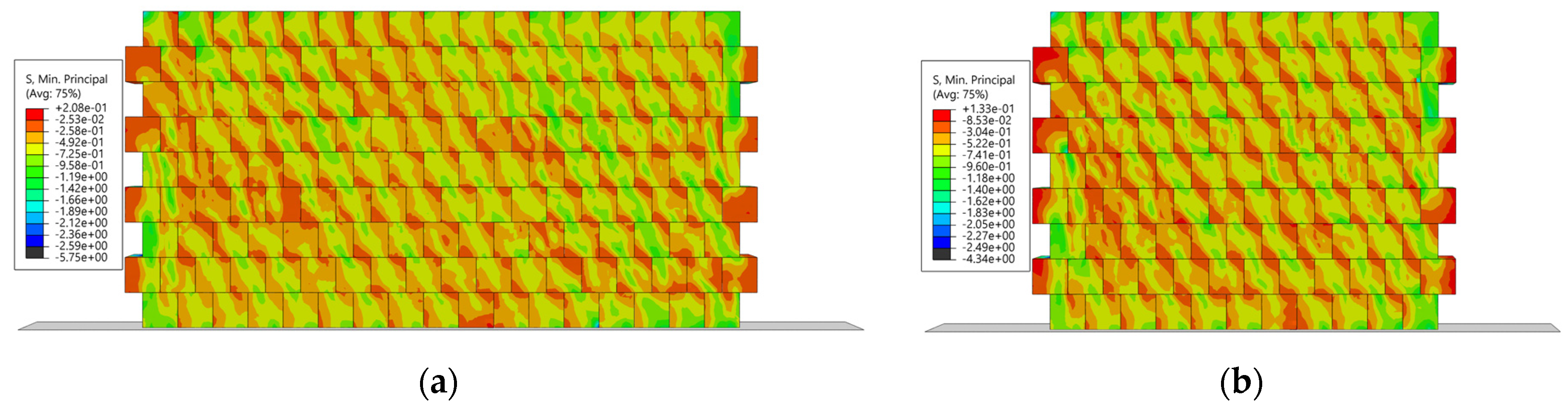
Figure 15 illustrates the distribution of minimum principal stresses at the maximum resistance for each of the considered CM wall configurations. The diagonal struts are clearly visible in the solid walls (SW_1 and SW_2), indicating an efficient transfer of forces through the masonry. Interestingly, the inclination and width of the struts are not affected by the aspect ratio, and appear to be only a function of the unit overlap between rows.

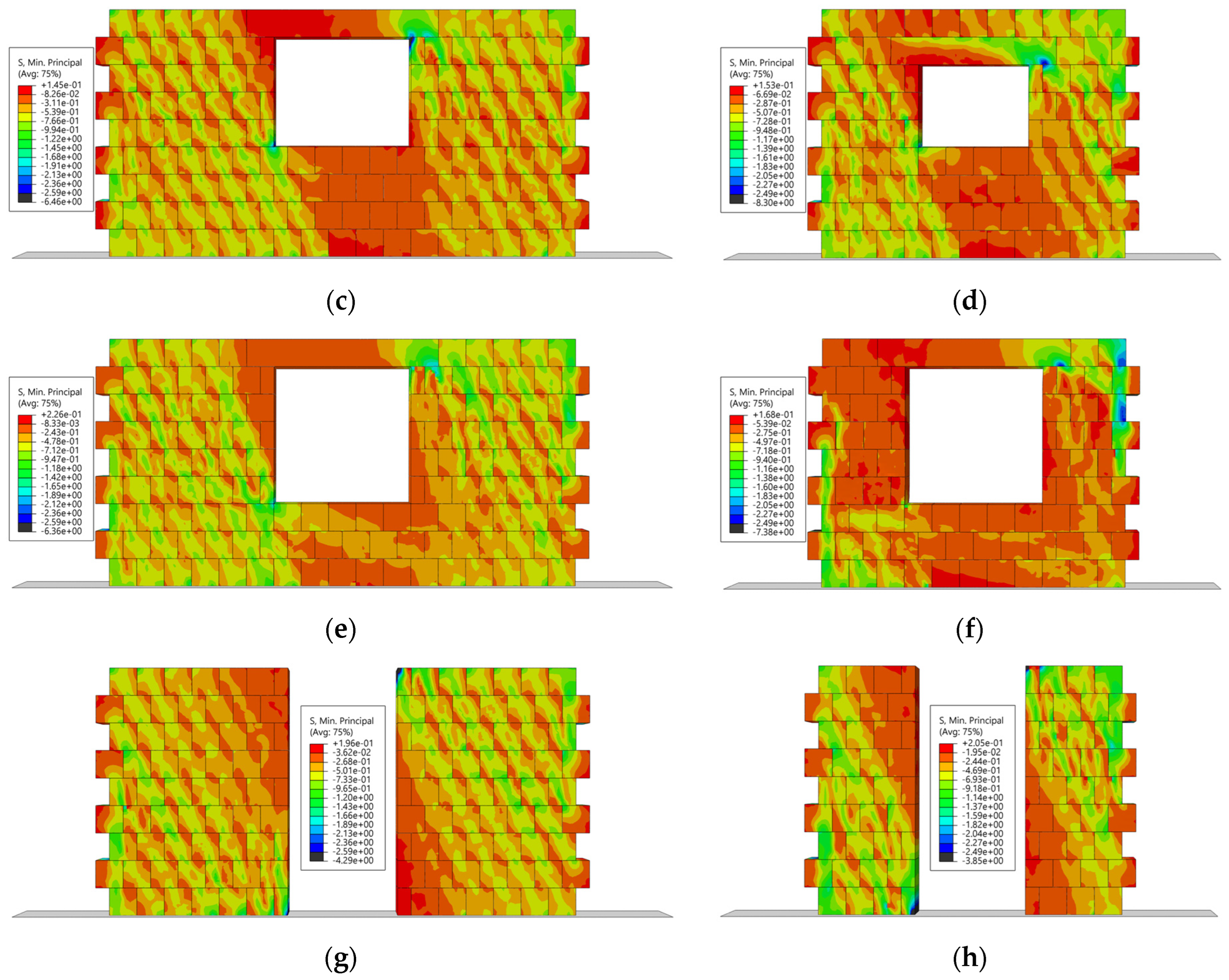
In CM walls with small openings, such as CWop_1 and CWop_2 (Figure 15c,d), the stress flow is interrupted around the openings. Diagonal struts are observed to the left and right of the central window, but no stress bands form directly around the opening. Instead, stress concentrations occur at the corners of the window, particularly near the top and bottom edges. A similar pattern is evident in CM walls with larger openings (A_p = 1.56 m²), such as CWopEC_1 and CWopEC_2 (Figure 15e,f). For CWopEC_2, with an AR of 0.71 (Figure 15f), the diagonal struts are no longer clearly visible.

For walls with door openings, such as CDop_1 and CDop_2, stress concentrations become evident around the lower-right and upper-left edges of the door openings, as seen in Figure 15g,h. These zones act as critical areas for stress accumulation, disrupting the continuity of the stress flow and significantly reducing the overall efficiency of force transfer through the wall.

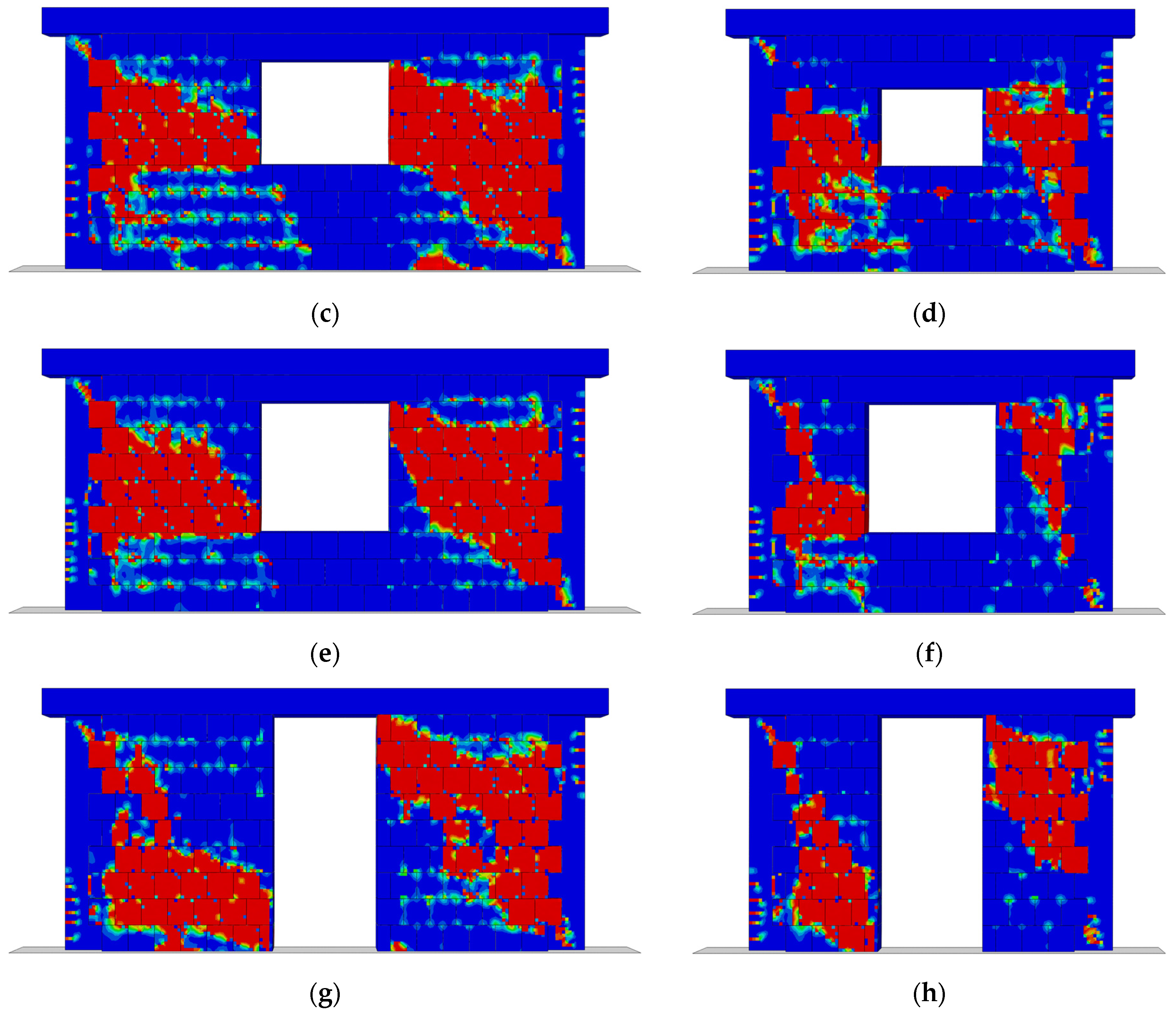
The damage patterns for the eight considered walls at 1.0% drift, illustrated in Figure 16, align closely with the stress distribution results. Solid CM walls (SW1, Figure 16a, and SW2, Figure 16b) exhibit distributed diagonal cracking, while walls with smaller openings, i.e., CWop_1 and CWop_2 (Figure 16c,d, respectively), show concentrated damage around the openings. The damage occurs primarily at the corners of the openings, with diagonal cracks extending toward the RC confining elements. Walls with door openings (CDop_1, CDop_2) show asymmetric damage through the wall.

The damage patterns in the tie-columns are consistent across all the considered configurations, showing bending damage concentrated at the lower part of the tie-columns. Additionally, a diagonal crack develops from the masonry into the upper corners of the RC tie-columns, eventually leading to shear failure within the tie-columns. This shear failure of tie-columns, however, does not appear to affect the pushover curves, which show no sudden drops.

4.1.2. Position of Window Opening

To further investigate the influence of window opening position on the seismic response of CM walls, four more configurations were analyzed by shifting the window opening left and right while keeping the opening size constant ($O_p=10\%$ for AR = 0.5, and $O_p=8.6\%$ for AR = 0.71), as shown in Figure 17. These configurations enabled the assessment of how shifting the window opening influenced the overall reduction in strength and damage patterns.

The pushover curves for the CM walls with varying window opening positions are presented in Figure 18. The results indicate that shifting the window opening affects both the peak base shear and the overall seismic response, but not by much. For walls with AR = 0.5 (Figure 18a), the left LWop_1 and right RWop_1 exhibit slightly higher strength compared to the centrally positioned window (CWop_1). A similar trend is observed for walls with AR = 0.71 (Figure 18b), where LWop_2 and RWop_2 demonstrate better performance compared to the CWop_2 wall configuration in terms of peak strength.

Interestingly, walls with a window opening on the right side (RWop_1 and RWop_2) exhibit a notable drop in capacity at larger drift levels. Specifically, for both aspect ratios, the pushover curves for the RWop configurations fall below those for the CWop and LWop configurations at approximately 0.8% drift. In case of an earthquake, the load acts in the push and pull directions, which means that the worst performing response indicates the expected result. In addition, the post-peak response of walls with offset openings is clearly worse than of those with cantered openings.

The observed differences in capacity can be partially attributed to the distribution of damage and the available wall area for diagonal strut formation. Damage patterns for these configurations at 1.0% drift are shown in Figure 19. For walls with a central opening, i.e., CWop_1 and CWop_2 (see Figure 16c,d, respectively), the reduced wall area around the opening limits the development of diagonal struts, leading to a lower base shear capacity compared to configurations with shifted openings. In contrast, when the window opening is shifted to the left or right, a larger portion of the wall becomes active in resisting the lateral (seismic) loads, resulting in slightly higher strengths for the LWop and RWop configurations.

4.1.3. Strength Reduction Factor for CM Walls Without Internal Tie-Columns

The strength reduction factor ($R_S$) is defined as the ratio of the strength of a wall with openings to that of a solid wall, and is one of the most important parameters for design. The obtained strength reduction values, according to the FEM model used in this study, were compared to the predictions of the model of Al-Chaar et al. [42] and the model of Basha et al. [43], as shown in

Table 5. Strength reduction factor.

Model No.	Model Name	${\mathit{F}}_{\mathit{m}\mathit{a}\mathit{x},\mathit{n}\mathit{u}\mathit{m}}$ [kN]	${\mathit{R}}_{\mathit{s}}$ [-]	${\mathit{A}}_{\mathit{r}}$ [-]	${\mathit{R}}_{\mathit{s},\mathit{A}\mathit{l}-\mathit{C}}$ [-]	${\mathit{R}}_{\mathit{s},\mathit{B}\mathit{A}}$ [-]	${\mathit{R}}_{\mathit{s},\mathit{A}\mathit{l}-\mathit{C}}/{\mathit{R}}_{\mathit{S}}$ [-]	${\mathit{R}}_{\mathit{s},\mathit{B}\mathit{A}}/{\mathit{R}}_{\mathit{S}}$ [-]
1	SW_1	454.33	1.0	0.0	1.0	1.0	1.0	1.0
3	CWop_1	348.71	0.77	0.1	0.85	0.78	1.10	1.01
5	CWopEC_1	332.97	0.73	0.125	0.81	0.74	1.10	1.01
7	CDop_1	316.26	0.70	0.18	0.73	0.67	1.05	0.97
9	LWop_1	359.61	0.79	0.1	0.85	0.78	1.07	0.98
11	RWop_1	368.87	0.81	0.1	0.85	0.78	1.04	0.96
2	SW_2	339.88	1.0	0.0	1.0	1.0	1.0	1.0
4	CWop_2	261.53	0.77	0.086	0.87	0.80	1.13	1.04
6	CWopEC_2	212.06	0.62	0.179	0.73	0.67	1.18	1.08
8	CDop_2	206.23	0.61	0.257	0.63	0.59	1.04	0.97
10	LWop_2	278.08	0.82	0.086	0.87	0.80	1.06	0.97
12	RWop_2	282.82	0.83	0.086	0.87	0.80	1.04	0.96

. Both models are explicit functions of the ratio of opening area to the area of the CM wall panel $A_r$. The model of Al-Chaar et al. [42] is given as follows:

$$R_{s,Al-C}=0.6 A_r^2-1.6 A_r+1$$

(15)

whereas the model of Basha et al. [43] is given as follows:

$$R_{s,BA}=1-A_r^{0.65}$$

(16)

The performance of both models is compared in Figure 20, which indicates that the model of Basha et al. [43] aligns better with the results of the FEM analyses.

4.2. Effect of Internal Tie-Columns

4.2.1. Walls with Windows

The considered wall configurations with two sizes of internal tie-columns (15 × 15 cm and 25 × 25 cm) are illustrated in Figure 21.

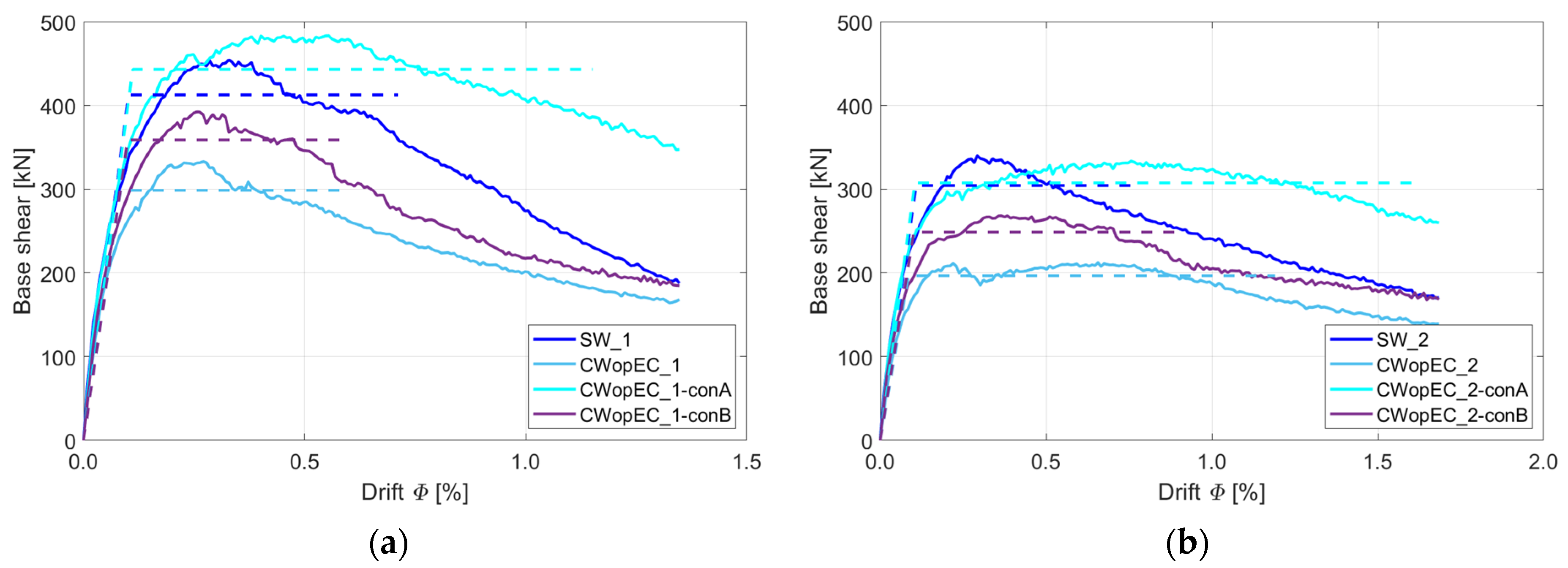
The pushover curves shown in Figure 22 show how much RC tie-columns around window openings improve peak strength and drift at peak strength, with larger tie-columns providing substantially larger improvements, as well as better post-peak behaviour.

For walls with AR = 0.5, the model with 25 × 25 cm tie-columns (cyan solid curve in Figure 22a) demonstrates an increase in peak strength of 45% relative to the model without tie-columns (light blue curve, Figure 22a). The drift at maximum strength is increased by 212%, from 0.26% for the model CWopEC_1 to 0.55% for the model CWopEC_1-conA. In contrast, the model with smaller 15 × 15 cm tie-columns demonstrates a more modest improvement, with an 18% improvement in strength and no change in drift at peak strength.

Similarly, for walls with AR = 0.71, the model with 25 × 25 cm tie-columns shows a 57% increase in peak strength (cyan and blue light solid curve in Figure 22b) and a 330% increase in drift at maximum strength. This notable increase in drift also highlights the enhanced ductility of the CM wall. On the other hand, the model with 15 × 15 cm tie-columns demonstrates a more limited improvement, with a 26% increase in peak strength and a 61% increase in drift, from 0.23% to 0.37%.

It is interesting to note that the addition of 25 × 25 cm tie-columns around window openings improves the seismic performance of the walls even compared to the solid wall. For walls with AR = 0.5, the strength increases by 7% compared to SW_1. For walls with AR = 0.71, 25 × 25 cm tie-columns give almost identical strength compared to the solid wall (SW_2).

To estimate the effect of tie-column sizes on the ductility of the considered walls with window openings, the response curves were idealized into bilinear curves, as shown in Figure 22. The idealization was performed by assuming stiffness at 60% of the peak strength, and the ultimate displacement at the point where the strength drops to 80% of its peak value. The idealized curve has equal energy to the original one (areas under both curves are the same). These results of the idealization are presented in

Table 6. Strength and ductility of CM walls with window openings and differently sized tie-columns around openings.

Model Name	Internal Tie-Column [cm]	Idealized Resistance [kN]	Relative to SW_1 [-]	Ductility [-]	Relative to SW_1 [-]
SW_1	-	412.6	-	7.0	-
CWopEC_1	-	298.6	0.72	7.0	1.00
CWopEC_1-conA	25 × 25	443.1	1.07	10.4	1.49
CWopEC_1-conB	15 × 15	358.8	0.87	5.8	0.83
SW_2	-	304.3	-	7.2	-
CWopEC_2	-	196.5	0.65	14.0	1.94
CWopEC_2-conA	25 × 25	307.5	1.01	15.5	2.15
CWopEC_2-conB	15 × 15	248.6	0.82	8.9	1.24

, and show that 25 × 25 cm tie-columns substantially improve ductility, whereas the effect is much less significant for walls with 15 × 15 cm tie-columns. Higher ductility indicates a much more gradual post-peak degradation and a higher capacity for energy dissipation.

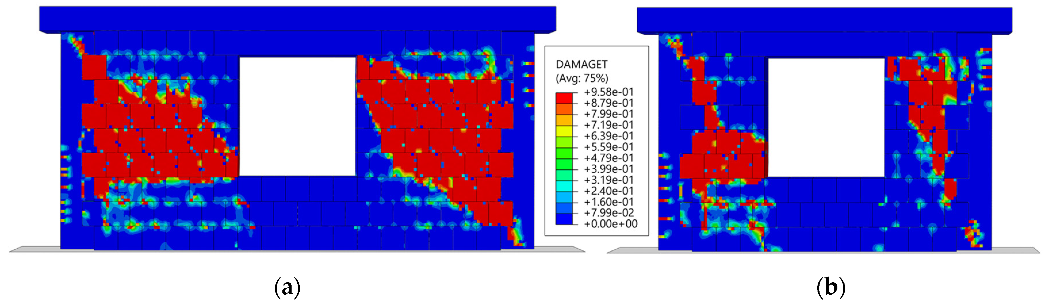
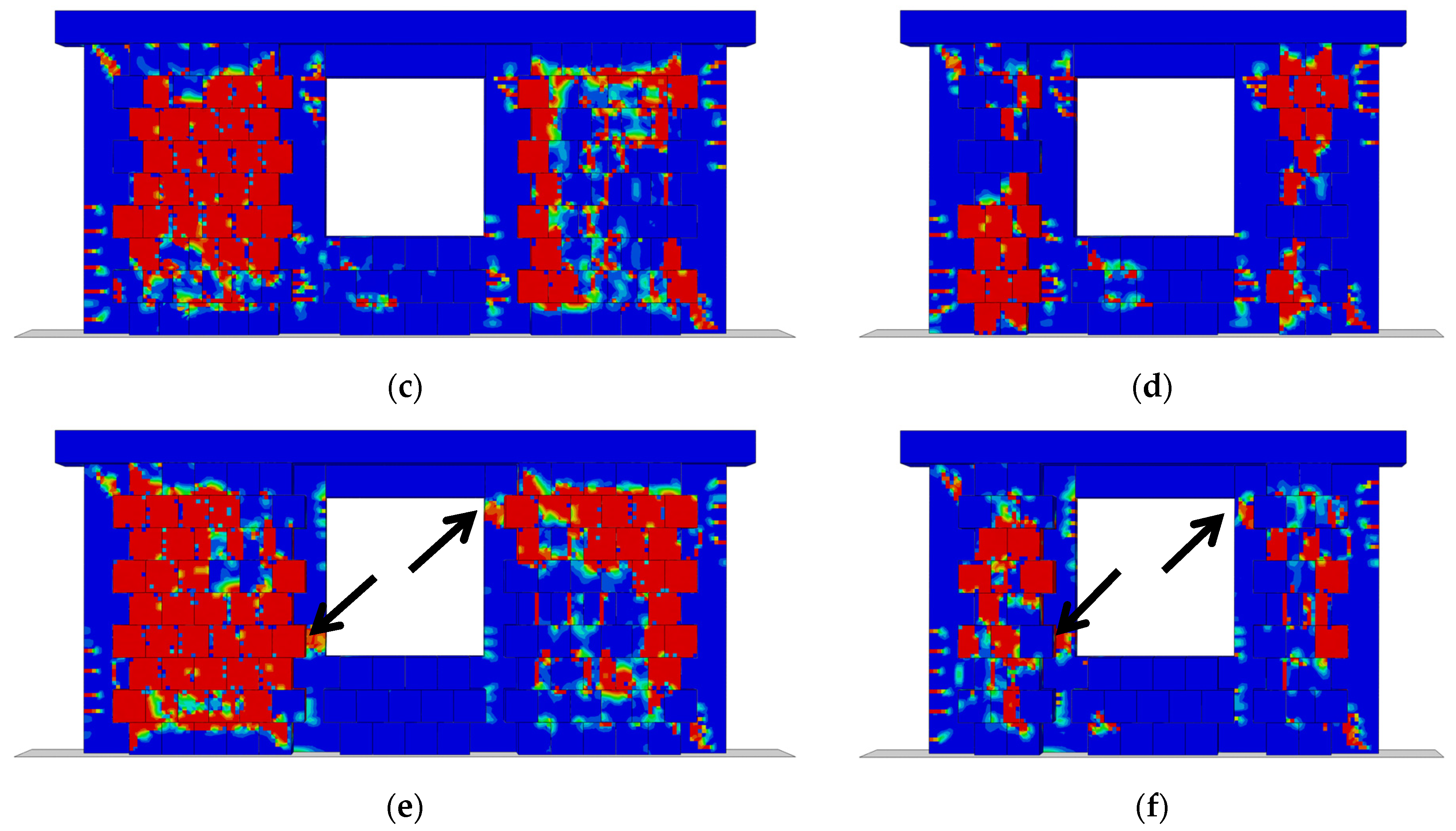
The damage patterns shown in Figure 23 highlight the key role of RC tie-columns in reducing and localizing damage around window openings. In models with tie-columns of 25 × 25 cm (Figure 23c,d), these confining elements effectively mitigated stress concentrations and prevented damage at the lower-left and upper-right corners of the window openings observed in the reference models (Figure 23a,b). In contrast, models with 15 × 15 cm tie-columns (Figure 23e,f) exhibited vast shear cracks at the lower-left and upper-right corners of the window for both ARs, as indicated by black arrows. Horizontal cracks were also observed at the lower end of the left tie-column and the upper end of the right tie-column, reflecting mixed-mode behaviour that combined flexural and shear damage in these elements.

Overall, the inclusion of larger tie-columns (25 × 25 cm) significantly improved the seismic performance of the walls by reducing damage concentrations, better distributing stress, and limiting crack propagation, compared to smaller tie-columns (15 × 15 cm) or reference models with unconfined window openings.

4.2.2. Walls with Doors

The configurations considered in this section are presented in Figure 24. RC tie-columns with dimensions of 25 × 25 cm and 15 × 15 cm were considered.

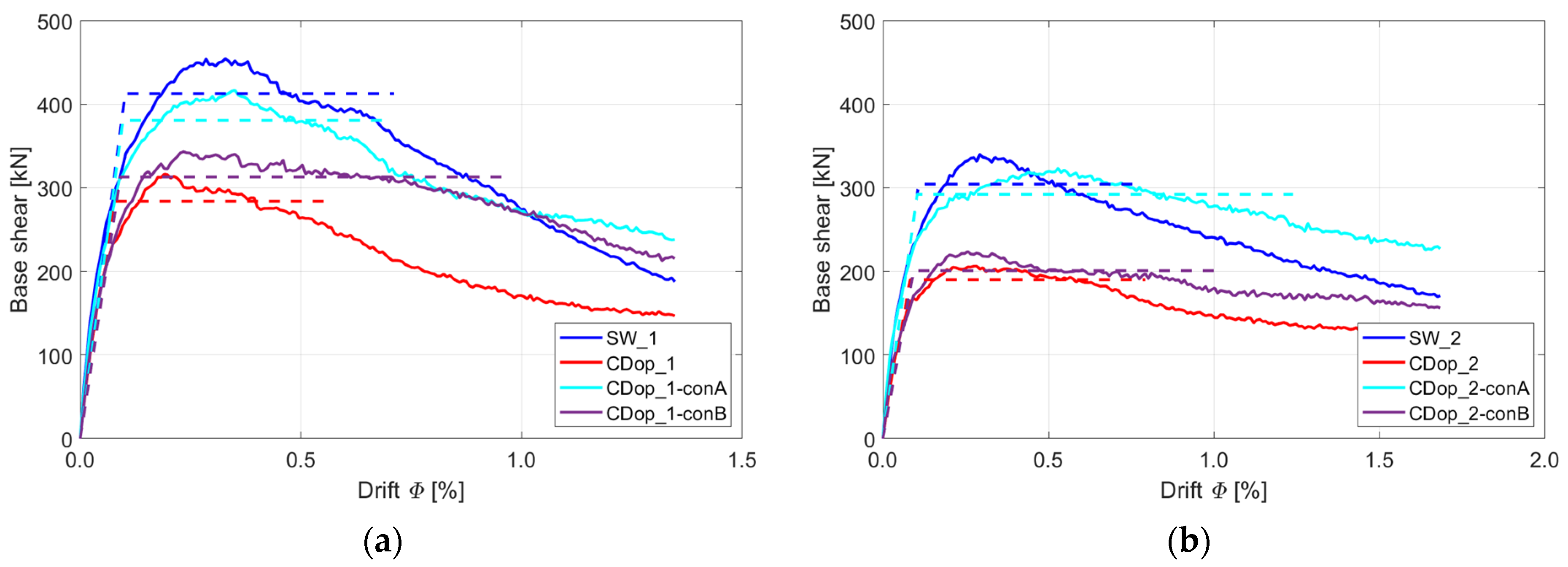
The pushover curves in Figure 25 highlight the crucial role of RC confining elements around door openings for preventing the degradation of the seismic performance of such walls. The models with larger tie-columns (25 × 25 cm) generally show superior performance compared to the model with 15 × 15 cm tie-columns. The difference in the post-peak region between models with 25 × 25 cm and 15 × 15 cm tie-columns is almost identical for walls with door openings (AR = 0.5). In contrast, for walls with the same AR but with window openings, the difference in post-peak behaviour is much more pronounced. However, it should be noted that the model with 25 × 25 cm tie-columns (AR = 0.71) shows greater ductility and improved post-peak behaviour.

The addition of 25 × 25 cm tie-columns in the wall with AR = 0.5 (cyan solid curve in Figure 25a) has increased peak strength by 32% compared to the base model (red curve in Figure 25a). Additionally, the drift at peak strength increases by 84%, rising from 0.19% in the reference model to 0.35% in the wall with 25 × 25 cm internal tie columns. In contrast, the smaller 15 × 15 cm tie-columns provide more modest improvements, with a 9% increase in strength and a 20% increase in drift level.

For walls with AR = 0.71, the model with 25 × 25 cm tie-columns shows a significant 57% increase in peak strength compared to the model without confinement around the opening (cyan and red solid curves in Figure 25b). In addition, the drift at peak strength rises by 204%, from 0.26% in the reference model to 0.53% in the model with internal tie-columns. The inclusion of 15 × 15 cm tie-columns leads to a slight improvement of 8% for both strength and drift at peak strength.

In contrast to the CM walls with window openings, where the addition of 25 × 25 cm tie-columns significantly enhances seismic performance (even exceeding that of the solid wall), the effect of this on walls with door openings is somewhat less pronounced. The models with 25 × 25 cm tie-columns in walls with AR = 0.5 and AR = 0.71 have ratios of peak strength compared to those of the reference walls of 0.92 and 0.95, respectively.

To analyze the effect of tie-columns sizes on ductility, the response curves were again idealized into bilinear curves, as depicted in Figure 25, with dashed lines in the same colours, to facilitate comparison. The corresponding values are summarized in

Table 7. Strength and ductility of CM walls with door openings and differently sized tie-columns around openings.

Model Name	Internal Tie-Column [cm]	Idealized Resistance [kN]	Relative to SW_1 [-]	Ductility [-]	Relative to SW_1 [-]
SW_1	-	412.6		7
CDop_1	-	283.8	0.69	7.32	1.05
CDop_1-conA	25 × 25	380.6	0.92	7.07	1.01
CDop_1-conB	15 × 15	312.9	0.76	10.73	1.53
SW_2	-	304.3		7.2
CDop_2	-	190.0	0.62	9.64	1.34
CDop_2-conA	25 × 25	292.1	0.96	11.96	1.66
CDop_2-conB	15 × 15	200.8	0.66	10.74	1.49

. In this case, the small tie-columns improved ductility for both ARs. The large tie-columns, on the other hand, were effective only for the wall with AR = 0.71.

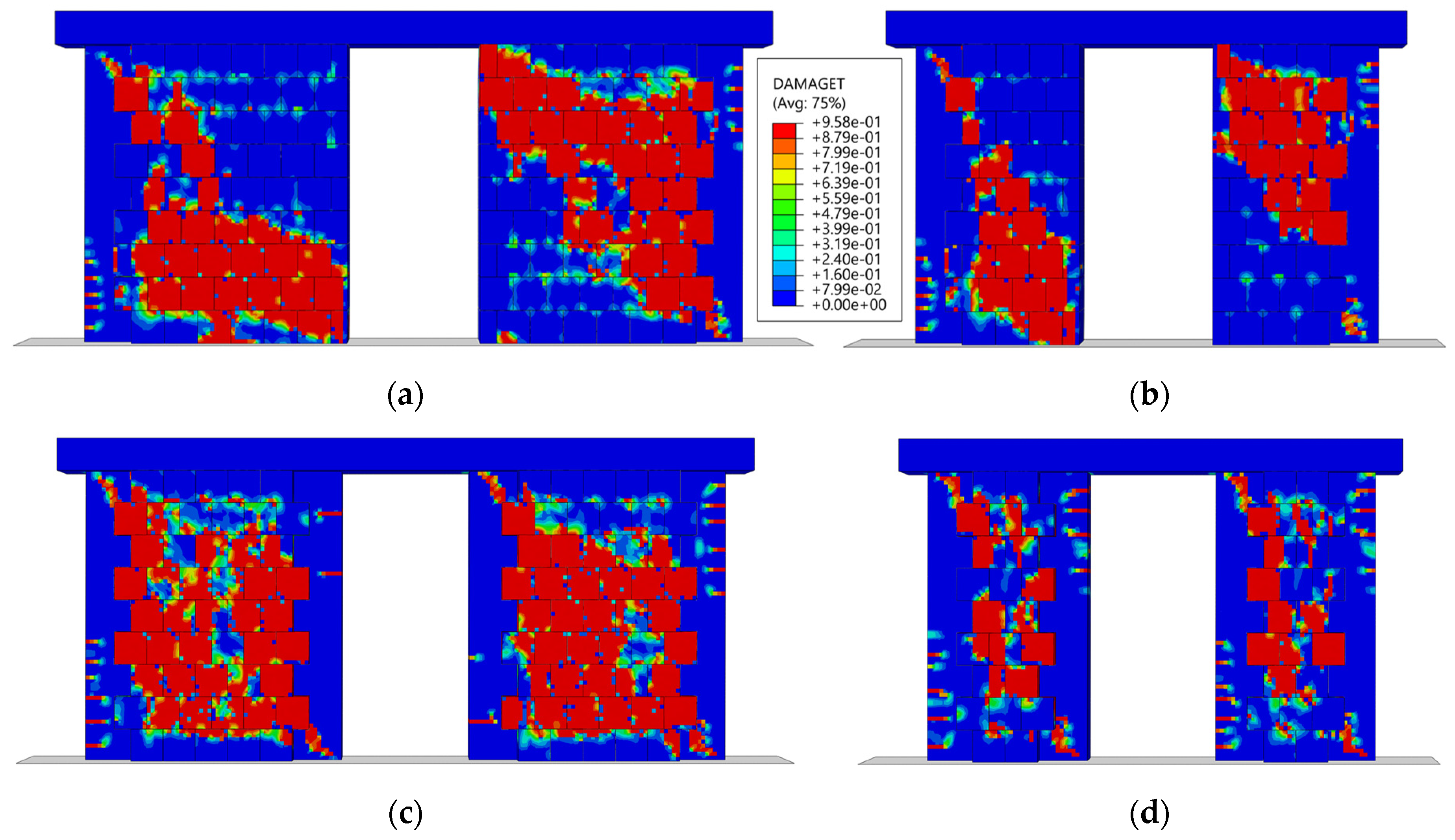
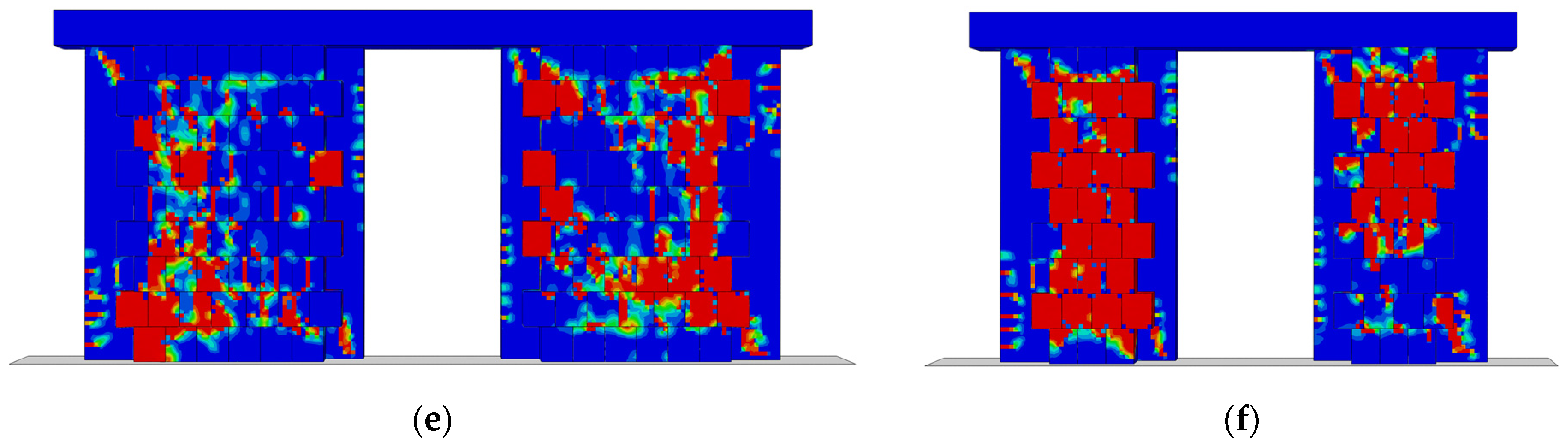
The damage distribution patterns, illustrated in Figure 26, reveal the role of RC tie-columns in managing stress concentration and localizing damage near door openings. Based on the results, similar observations can be made as for the CM walls with windows. For the model with AR = 0.5, which has 25 × 25 cm tie-columns (Figure 26c), more extensive damage is observed along the left and right piers, compared to the model with 15 × 15 cm tie-columns (Figure 26e). This includes shear cracks that extend from the masonry piers into the surrounding tie-columns, both externally and internally. Conversely, for the model with AR = 0.71 and 15 × 15 cm tie-columns, the damage is more widespread compared to the model with 25 × 25 cm tie-columns. Additionally, in the model with AR = 0.71 and 25 × 25 cm tie-columns, the internal tie-columns exhibit significantly more activity, with horizontal cracks observed at the upper part of the interior left column and the lower part of the interior right column, as seen in Figure 26c,d. It is believed that the damage patterns observed for these models with AR = 0.5 (25 × 25 and 15 × 15 cm tie-columns) are consistent with the behaviour seen in the post-peak region of the pushover curves, where nearly identical performance is noted for both models (cyan and purple solid curves in Figure 25a).

5. Conclusions

The paper studies the effects of openings and tie-columns on the response of CM walls using a validated micro-FEM model. The type of masonry considered in this study is novel, and has not been analyzed in this manner before.

The results indicate that openings have a very detrimental effect on the seismic performance of CM walls, regardless of their size. Even in cases when the area of the opening was less than 10% of the CM wall area, the resistance decreased by more than 15%. The post-peak response and ductility were affected as well. Additionally, the results show that adding tie-columns next to windows proves to be an effective measure for reducing the detrimental effect of openings. However, because the thickness of the considered masonry is 38 cm, the size of additional the tie-columns should be at least 25 × 25 cm. When smaller tie-columns were used (e.g., 15 × 15 cm), they were much less effective.

For walls with AR = 0.5, the model with 25 × 25 cm internal tie-columns showed an increase in peak strength of 45% relative to the model without tie-columns. The drift at maximum strength increased by 212%, from 0.26% for the model CWopEC_1 to 0.55% for the model CWopEC_1-conA. In contrast, the model with smaller 15 × 15 cm internal tie-columns demonstrated a more modest improvement, with an 18% improvement in strength and no change in drift at peak strength.

Similarly, for walls with AR = 0.71, the model with 25 × 25 cm internal tie-columns showed a 57% increase in peak strength and a 330% increase in drift at maximum strength. This notable increase in drift also highlights the enhanced ductility of this CM wall. On the other hand, the model with 15 × 15 cm internal tie-columns demonstrated a more limited improvement, with a 26% increase in peak strength and a 61% increase in drift, from 0.23% to 0.37%.

It has been shown in this paper that the strength reduction factor due to openings, as obtained from the present analysis, aligns quite well with the predictions of the model of Basha et al. [43], which confirms the suitability of this model for the considered type of masonry.

The position of the window opening in CM walls was also analyzed. It was determined that an offset position resulted in slightly greater strength due to clearer transfer of stresses in the masonry, but that this position resulted in worse post-peak behaviour due to the tie-columns being more stressed.

It should be noted that all of the conclusions presented here are relevant only for the considered type of masonry, and are solely based on numerical simulations. Further experimental tests should be conducted to fully validate these conclusions.

References

1. Pérez Gavilán, J.J.; Flores, L.; Alcocer, S. An Experimental Study of Confined Masonry Walls with Varying Aspect Ratios. Earthq. Spectra 2015, 31, 945–968. [Google Scholar] [CrossRef]
2. Moroni Yadlin, M.O.; Gomez, C.; Astroza, M. Confined Block Masonry Building. In A Report Prepared for the Confined Masonry Network; Earthquake Engineering Research Institute: Oakland, CA, USA, 2010. [Google Scholar]
3. Eurocode 8: Design of Structures for Earthquake Resistance—Part 1: General Rules, Seismic Actions and Rules for Buildings. Available online: https://www.phd.eng.br/wp-content/uploads/2015/02/en.1998.1.2004.pdf (accessed on 3 December 2024).
4. Marques, R.; Lourenço, P. Structural Behaviour and Design Rules of Confined Masonry Walls: Review and Proposals. Constr. Build. Mater. 2019, 217, 137–155. [Google Scholar] [CrossRef]
5. Gams, M.; Triller, P.; Jäger, A. In-plane seismic behaviour of URM and confined masonry built from vertically perforated blocks and polyurethane glue. Structures 2023, 58, 105528. [Google Scholar] [CrossRef]
6. Marques, R.; Pereira, J.M.; Lourenço, P.B. Lateral in-plane seismic response of confined masonry walls: From numerical to backbone models. Eng. Struct. 2020, 221, 111098. [Google Scholar] [CrossRef]
7. Borah, B.; Kaushik, H.B.; Singhal, V. Evaluation of modeling strategies for gravity and lateral load analysis of confined masonry structures. Bull. Earthq. Eng. 2022, 21, 1273–1301. [Google Scholar] [CrossRef]
8. DIANA FEA BV. DIANA FEA, 2017; DIANA FEA BV: Hague, The Netherlands. Available online: https://dianafea.com (accessed on 10 December 2024).
9. Abaqus. Abaqus/Explicit CAE, Dassault Systèmes Simulia Corp.: Providence, RI, USA, 2023. Available online: https://www.3ds.com/products/simulia/abaqus (accessed on 10 December 2024).
10. Weber, M.; Thoma, K.; Hofmann, J. Finite element analysis of masonry under a plane stress state. Eng. Struct. 2021, 226, 111214. [Google Scholar] [CrossRef]
11. Chourasia, A.; Singhal, S.; Chourasia, A. Numerical simulation of laterite confined masonry building subjected to quasi-static monotonic lateral loading. J. Struct. Integr. Maint. 2023, 8, 1–11. [Google Scholar] [CrossRef]
12. Lourenço, P.B. Computational Strategies for Masonry Structures. PhD Thesis, TU Delft, Delft, The Netherlands, 1996. [Google Scholar]
13. Gams, M.; Bohinc, U.; Tomaževič, M. Experimental tests and constitutive laws for unit-mortar interfaces. In Proceedings of the Vienna Congress on Recent Advances in Earthquake Engineering and Structural Dynamics, Vienna, Austria, 28 August–30 August 2013. [Google Scholar]
14. Tripathy, D.; Singhal, V. Estimation of in-plane shear capacity of confined masonry walls with and without openings using strut-and-tie analysis. Eng. Struct. 2019, 188, 290–304. [Google Scholar] [CrossRef]
15. Meguro, K.; Tagel-Din, H. Applied element method for structural analysis: Theory and application for linear materials. Struct. Eng. Earthq. Eng. 2000, 17, 21–35. [Google Scholar] [CrossRef]
16. Domaneschi, M.; Cimellaro, G.P.; Scutiero, G. A simplified method to assess generation of seismic debris for masonry structures. Eng. Struct. 2019, 186, 306–320. [Google Scholar] [CrossRef]
17. Meli, R.; Brzev, S.; Astroza, M.; Boen, T.; Crisafulli, F.; Dai, J.; Farsi, M.; Hart, T.; Mebarki, A.; Moghadam, A.S.; et al. Seismic Design Guide for Low-Rise Confined Masonry Buildings. In World Housing Encyclopedia Report; Earthquake Engineering Research Institute: Oakland, CA, USA, 2011. [Google Scholar]
18. Brzev, S.; Astroza, M.; Moroni Yadlin, M.O. Performance of Confined Masonry Buildings in the 27 February 2010 Chile Earthquake. In A Report Prepared for the Confined Masonry Network; Earthquake Engineering Research Institute: Oakland, CA, USA, 2010. [Google Scholar]
19. Brzev, S.; Mitra, K. Earthquake-Resistant Confined Masonry Construction, 3rd ed.; National Information Center on Earthquake Engineering: Kanpur, India, 2018. [Google Scholar]
20. Pérez Gavilán, J.J.; Brzev, S.; Quiun, D.; Ganzerli, S.; Espinosa Cazarin, E.; Reiter, M.; Borseth, M.; Olewski, B. Seismic behaviour and design of confined masonry buildings: A review. In Proceedings of the 14th Canadian Masonry Symposium, Montréal, QC, Canada, 16–20 May 2021. [Google Scholar]
21. Yáñez, F.; Astroza, M.; Holmberg, A.; Ogaz, O. Behavior of Confined Masonry Shear Walls with Large Openings. In Proceedings of the 13th World Conference on Earthquake Engineering, Vancouver, BC, Canada, 1–6 August 2004. [Google Scholar]
22. Kuroki, M.; Kikuchi, K.; Nonaka, H.; Shimosako, M. Experimental Study on Reinforcing Methods Using Extra RC Elements for Confined Masonry Walls with Openings. In Proceedings of the 15th World Conference on Earthquake Engineering, Lisbon, Portugal, 24–28 September 2012. [Google Scholar]
23. Gupta, A.; Singhal, V. Experimental investigation of confined masonry walls with openings. J. Struct. Eng. 2024, 150, 04024136. [Google Scholar] [CrossRef]
24. Okail, H.; Abdelrahman, A.; Abdelkhalik, A.; Metwaly, M. Experimental and analytical investigation of the lateral load response of confined masonry walls. HBRC J. 2016, 12, 33–46. [Google Scholar] [CrossRef]
25. Maheri, M.R.; Moslemi, A.; Najafgholipour, M.A. The effects of brick wall and RC tie variables on the seismic performance of low-rise confined masonry buildings. J. Build. Eng. 2024, 95, 110289. [Google Scholar] [CrossRef]
26. Shandilya, A.N.; Kumar, V.; Haldar, A.; Mandal, S. Influence of opening shape, size and position on the ultimate strength, stiffness and energy dissipation of confined brick masonry walls. Bull. Earthq. Eng. 2024, 22, 7015–7045. [Google Scholar] [CrossRef]
27. Eurocode 6: Design of Masonry Structures—Part 1-1: Genereal Rules for Reinforced and Unreinforced Masonry Structures. Available online: https://www.phd.eng.br/wp-content/uploads/2015/02/en.1996.1.1.2005.pdf (accessed on 3 December 2024).
28. Tomaževič, M. Earthquake-Resistant Design of Masonry Buildings; Imperial College Press: London, UK, 1999. [Google Scholar]
29. Krtinić, N.; Gams, M.; Marko, M. Experimental and numerical investigation of the seismic response of confined masonry walls. In Proceedings of the 9th International Conference on Computational Methods in Structural Dynamics and Earthquake Engineering (COMPDYN), Athens, Greece, 12–14 June 2023. [Google Scholar]
30. Stavridis, A.; Shing, P.B. Finite-element modeling of nonlinear behavior of masonry-infilled RC frames. J. Struct. Eng. 2010, 136, 285–296. [Google Scholar] [CrossRef]
31. Nazir, S.; Dhanasekar, M. A non-linear interface element model for thin layer high adhesive mortared masonry. Comput. Struct. 2014, 144, 23–39. [Google Scholar] [CrossRef]
32. Kaushik, H.B.; Rai, D.C.; Jain, S.K. Stress-strain characteristics of clay brick masonry under uniaxial compression. J. Mater. Civ. Eng. 2007, 19, 728–739. [Google Scholar] [CrossRef]
33. Marinković, M.; Butenweg, C. Numerical analysis of the in-plane behaviour of decoupled masonry infilled RC frames. Eng. Struct. 2022, 272, 114959. [Google Scholar] [CrossRef]
34. Lubliner, J.; Oliver, J.; Oller, S.; Oñate, E. A plastic-damage model for concrete. Int. J. Solids Struct. 1989, 25, 299–326. [Google Scholar] [CrossRef]
35. Lee, J.; Fenves, G.L. Plastic-damage model for cyclic loading of concrete structures. J. Eng. Mech. 1998, 124, 892–900. [Google Scholar] [CrossRef]
36. Pavlović, M. Resistance of Bolted Shear Connectors in Prefabricated Steel-Concrete Composite Decks. PhD Thesis, Faculty of Civil Engineering, University of Belgrade, Belgrade, Serbia, 2013. [Google Scholar]
37. Eurocode 2: Design of Concrete Structures—Part 1-1: General Rules and Rules for Buildings. Available online: https://www.phd.eng.br/wp-content/uploads/2015/12/en.1992.1.1.2004.pdf (accessed on 3 December 2024).
38. Hordijk, A. Tensile and tensile fatigue behavior of concrete; experiments, modeling and analyses. Heron 1992, 37, 3–79. Available online: https://trid.trb.org/View/366922 (accessed on 15 December 2024).
39. CEB-FIP. CEB-FIP Model Code 2010. In Model Code for Concrete Structures; International Federation for Structural Concrete (fib): Lausanne, Switzerland, 2010. [Google Scholar]
40. López Almansa, F.; Alfarah, B.; Oller Martínez, S.H. Numerical simulation of RC frame testing with damaged plasticity model. Comparison with simplified models. In Proceedings of the 2nd European Conference on Earthquake Engineering and Seismology, Istanbul, Turkey, 24–29 August 2014. [Google Scholar]
41. Krtinić, N.; Marinković, M.; Gams, M. Numerical investigation of the seismic response of a new confined masonry system. J. Build. Eng. 2024; submitted for publication. [Google Scholar]
42. Al-Chaar, G.; Lamb, G.; Abrams, D. Effect of openings on structural performance of unreinforced masonry infilled frames. ACI Spec. Publ. 2003, 211, 247–262. [Google Scholar]
43. Basha, S.H.; Surendran, S.; Kaushik, H.B. Empirical models for lateral stiffness and strength of masonry-infilled RC frames considering the influence of openings. J. Struct. Eng. 2020, 146, 04020021. [Google Scholar] [CrossRef]
Figure 1. (a) Masonry unit (dimensions in millimetres) and (b) application of PU glue.
Buildings 15 00424 g001
Figure 2. (a) Geometry of CM wall test specimen (all dimensions in cm); (b) wall and tie-column reinforcement [5].
Buildings 15 00424 g002
Figure 3. LSs of tested CM wall specimen W8, identified with DIC system: (a) damage LS, (b) max. resistance LS, and (c) near-collapse LS. Red colour indicates cracks, while blue colour indicates undamaged area. Adapted from Krtinić et al. [29].
Buildings 15 00424 g003
Figure 4. (a) Experimental envelope curves of tested CM walls (W7 and W8), with different LSs highlighted; damage to protruding masonry due to tie-columns during test at (b) 0.5% and (c) 1.3% drift.
Buildings 15 00424 g004
Figure 5. Schematic representation of FE model built in Abaqus: (a) geometry and (b) loads.
Buildings 15 00424 g005
Figure 6. Mesh of FE model.
Buildings 15 00424 g006
Figure 7. CM wall with defined interaction properties.
Buildings 15 00424 g007
Figure 8. (a) Stress–strain curve for concrete under compression; (b) stress–displacement curve for concrete under tension. Uppercase letters indicate characteristic points on the graphs.
Buildings 15 00424 g008
Figure 9. (a) Stress–strain curve for masonry units in compression; (b) stress–displacement curve for masonry units in tension. Uppercase letters indicate characteristic points on the graphs.
Buildings 15 00424 g009
Figure 10. Damage evolution curves for concrete: (a) compression and (b) tension.
Buildings 15 00424 g010
Figure 11. Damage evolution curves for masonry units: (a) compression and (b) tension.
Buildings 15 00424 g011
Figure 12. Numerical vs. experimental force–drift envelope curves.
Buildings 15 00424 g012
Figure 13. Typical CM wall configurations: (a) SW_1, (b) SW_2, (c) CWop_1, (d) CWop_2, (e) CWopEC_1, (f) CWopEC_2, (g) CDop_1, and (h) CDop_2.
Buildings 15 00424 g013aBuildings 15 00424 g013b
Figure 14. Pushover curves for CM walls with different size of openings: (a) AR = 0.5 and (b) AR = 0.71.
Buildings 15 00424 g014
Figure 15. Distribution of minimum principal stresses at drift corresponding to max. resistance of considered CM wall configurations: (a) SW_1, (b) SW_2, (c) CWop_1, (d) CWop_2, (e) CWopEC_1, (f) CWopEC_2, (g) CDop_1, and (h) CDop_2.
Buildings 15 00424 g015aBuildings 15 00424 g015b
Figure 16. Damage patterns for considered wall configurations at 1.0% drift: (a) SW_1, (b) SW_2, (c) CWop_1, (d) CWop_2, (e) CWopEC_1, (f) CWopEC_2, (g) CDop_1, and (h) CDop_2.
Buildings 15 00424 g016aBuildings 15 00424 g016b
Figure 17. CM wall configurations: (a) LWop_1, (b) LWop_2, (c) RWop_1, and (d) RWop_2.
Buildings 15 00424 g017
Figure 18. Pushover curves for CM walls with different positions of window openings: (a) AR = 0.5 and (b) AR = 0.71.
Buildings 15 00424 g018
Figure 19. Damage patterns for considered opening positions in wall configurations at 1.0% drift: (a) LWop_1, (b) LWop_2, (c) RWop_1, and (d) RWop_2.
Buildings 15 00424 g019
Figure 20. Effect of openings on R s and comparison to models of Al-Chaar et al. [42] (black solid line) and Basha et al. [43] (black dashed line).
Buildings 15 00424 g020
Figure 21. CM wall configurations: (a) CWopEC_1-conA, (b) CWopEC_2-conA, (c) CWopEC_1-conB, and (d) CWopEC_2-conB.
Buildings 15 00424 g021aBuildings 15 00424 g021b
Figure 22. Pushover curves for CM walls (with window opening) with or without vertical confinement around openings: (a) AR = 0.5 and (b) AR = 0.71. Bilinear curves are marked with dashed lines in same colour.
Buildings 15 00424 g022
Figure 23. Damage patterns for considered CM wall configurations at 1.0% drift: (a) CWopEC_1, (b) CWopEC_2, (c) CWopEC_1-conA, (d) CWopEC_2-conA, (e) CWopEC_1-conB, and (f) CWopEC_2-conB. Black arrows indicate shear cracks in the internal tie-columns.
Buildings 15 00424 g023aBuildings 15 00424 g023b
Figure 24. CM wall configurations: (a) CDop_1-conA, (b) CDop_2-conA, (c) CDop_1-conB, and (d) CDop_2-conB.
Buildings 15 00424 g024
Figure 25. Pushover curves for CM walls (with door opening) with or without vertical confinement around openings: (a) AR = 0.5 and (b) AR = 0.71. Bilinear curves are marked with dashed lines in same colour.
Buildings 15 00424 g025
Figure 26. Damage patterns for considered CM wall configurations at 1.0% drift: (a) CDop_1, (b) CDop_2, (c) CDop_1-conA, (d) CDop_2-conA, (e) CDop_1-conB, and (f) CDop_2-conB.
Buildings 15 00424 g026aBuildings 15 00424 g026b