An Optimization Procedure for Improving the Prediction Performance of Failure Assessment Model

Abstract

Improving the Prediction Performance (PP) of crack pipeline Failure Assessment Model (FAM) is of great significance for the safety of pipeline structure and engineering. However, conventional optimizations for PP always focus on either safety or accuracy, failing to balance the overall requirements of structural applications. Therefore, this paper proposes an optimization procedure for comprehensively improving FAM’s PP. The establishment of the procedure can be divided into three parts: 1. setting a rational and robust optimization target, where the Improved Guo-Ni Model (IGNM) is raised to provide an absolute score s for fully quantifying FAM’s PP in terms of the multi-dimensional performances, including stability and Distributional Location Characterizations (DLCs) of FAM’s prediction results; 2. determining the candidate solutions which are selected as the Critical Safety Factor (CSF) values related to FAM’s prediction confidence level (R₁) in this paper; 3. constructing the optimization framework based on the Particle Swarm Optimization algorithm to search for the optimal CSF (OCSF) that can maximize s. Finally, empirical verification results show that the procedure enhances the overall s values of BS 7910:2019 and CorLAS models by 3.32% and 6.09%, respectively, through balancing DLCs, which increases the applicability of FAM across different projects and provides a new approach for the optimization control of FAM’s overall performance.

1. Introduction

Pipelines are of great practical value in industrial construction and energy transportation [1,2]. However, during pipeline operation, the structure may develop axial cracks on the external surface under high-pressure conditions, which destroys structural integrity and severely threatens engineering safety [3,4]. Therefore, developing high-quality Failure Assessment Models (FAMs) for cracked pipelines is significant for evaluating structural reliability and reducing accident risks. Until now, many highly recognized FAMs have been developed to assess the integrity, reliability and safety of pipelines [5], such as GB/T 2019 [6], BS 7910:2019 [7], Battelle [8], CorLAS [9], etc. However, different FAMs lead to varying results, making it necessary to evaluate and optimize FAM’s Prediction Performance (PP) for improving their availability.

To assess FAM’s PP, many scholars have already conducted lots of studies with various assessment criteria. For instance, Cosham et al. [10] used means and variance to evaluate FAM’s accuracy. Yan et al. [8] employed means and coefficient of variation (COV) to research the FAM error. Yan et al. [11] utilized the mean and standard deviation of 12 in-service and 63 hydrostatic test pipe ruptures to explore the distinct performance characteristics of seven FAMs. Guo et al. [12] proposed seven indicators to comprehensively investigate FAM’s PP based on 250 cracked pipeline experiments. Notably, in contrast to previous studies which employed simple statistical parameters to compare PP differences among FAMs, Guo et al.’s indicators contain stability and Distribution Location Characteristics (DLCs), which can more fully and effectively meet the practical application requirements of FAMs. Therefore, the subsequent PP quantification model Guo-Ni Model (GNM) proposed by Guo et al. [13], which established an Evaluation Indicator System (EIS) based on the above indicators, also demonstrated significant advantages in evaluation comprehensiveness and engineering guidance. However, the GNM treats PP quantification as a multi-criteria decision-making problem, and its evaluation results are subject to the type of decision-making model employed, which implies that GNM fails to establish a unified performance standard. This limits its applicability in PP optimization. Hence, the Improved Guo-Ni Model (IGNM) is proposed in this paper to directly present PP with a single final score, which simultaneously takes four multi-criteria decision-making models, including Sum Weight Method (SWM) [14], Technique for Oder Preference by Similarity to the Ideal Solution (TOPSIS) [15], Vlsekriterijumska Optimizacija I Kompromisno Resenjie (VIKOR) [16] and Preference Ranking Organization Method for Enrichment of Evaluations II (PROMETHEE II) [17] into account, thereby providing a robust and comprehensive optimization objective for PP enhancement. This transition from FAM’s pure evaluation to systematic optimization guidance constitutes the core theoretical innovation of this paper.

As for the optimization of FAM’s PP, traditional methods always rely on adjusting prediction results by the Critical Safety Factor, i.e., the ratio of recommended predicted to experimental values [18]. However, this way aims to control prediction risk, and it tends to yield overly conservative results, leading to material wastage, which significantly impedes models’ widespread acceptance and utilization within the engineering field. Moreover, to optimize the prediction accuracy, numerous novel FAMs have been developed for failure prediction in recent years. For instance, Kiswendsida et al. [19] corrected the prediction results of the modified Ln-Sec mode [20] by introducing a correction factor and the effect of correction was evaluated based on the model error standard deviation, thereby enhancing prediction accuracy. Su et al. [21] proposed a multi-layer deep neural network (DNN) model and analyzed the influences of DNN model parameters on the prediction accuracy of failure pressure for defective pipelines. Sun et al. [22] employed multiple machine learning models to predict failure modes in pipeline structures containing longitudinal surface cracks. Ren et al. [23] developed the Genetic Algorithm-Back Propagation Neural Network prediction model to assess pipeline safety. Huang et al. [24] built a hybrid network model based on Convolutional Neural Network (CNN) and Bidirectional Gated Recurrent Unit (BiGRU), while introducing the Squeeze-and-Excitation (SE) mechanism to optimize features within the convolutional module, thereby significantly enhancing the efficacy of structural damage identification. However, these FAMs focus on minimizing errors while neglecting other practical requirements for PP optimization, making them fail to balance the conservatism, riskiness and robustness of prediction results and constraining the practical applicability of models. Essentially, the limitations of previous PP optimization studies partly stem from basing optimization on incomplete PP assessment, which hinders the ability to balance the overall requirements of structural applications. There is an urgent need to propose a procedure that can fully optimize FAM’s PP.

Therefore, this paper presents an optimization procedure for comprehensively improving FAM’s PP based on IGNM and Particle Swarm Optimization (PSO) [25]. Here, IGNM is raised to set the fitness for optimization, which can provide an absolute score s for fully quantifying FAM’s PP by integrating the multi-dimensional performance in FAM’s prediction results. PSO is used to build an iterative framework for searching the optimal overall PP, consisting of candidate solutions and fitness which are defined based on CSF and the overall s, respectively. Notably, PSO exhibits well-proven efficacy in solving continuous single-objective optimization problems, which aligns perfectly with the one-dimensional search requirement for optimal CSF (OCSF) in this paper. Compared to other intelligent algorithms such as Genetic Algorithms (GA) [26], Sailfish Optimization (SFO) [27] and Moth-Flame Optimization (MFO) [28], PSO is generally more easily implemented and converges faster when dealing with low-dimensional smooth problems. Therefore, considering both research target and computational cost, PSO is selected as the optimization tool for this procedure. Finally, it is verified through case study that the procedure can effectively enhance FAM’s PP by balancing DLCs including risk, conservatism, robustness and accuracy, which provides a new idea for the optimization control of FAM’s overall performance.

The paper is organized as follows: after introduction, the establishment principles and flowchart of IGNM are presented in Section 2. Section 3 gives PSO’s theory and Section 4 introduces the PP optimization procedure by its basic definitions and flowchart. Section 5 gives the case study to show the rationality of fitness setting, the optimization effect and the applicability for different preferences of the procedure. Section 6 presents the conclusions.

2. Improved Guo-Ni Model (IGNM)

Improved Guo-Ni Model (IGNM) is an enhanced quantification model for FAM’s Prediction Performance (PP) based on the Guo-Ni Model (GNM) [13], which can present PP directly with an overall score covering four different multi-criteria decision-making models’ results. In this section, IGNM is presented by the establishment principles and the flowchart to illustrate the acquisition of the final score.

2.1. Establishment Principles

The establishment principles of IGNM can be divided into three parts, including Evaluation Indicator System (EIS), Evaluation Mathematical Models (EMMs) and integration processing as presented in this section.

2.1.1. Evaluation Indicator System (EIS)

Evaluation Indicator System (EIS) raised by Guo. et al. in 2022 [13] is the basis of IGNM scoring, which provides comprehensive assessment criteria for quantifying PP. EIS consists of two aspects: stability (correlation C₁, multi-modality C₂ and dispersion C₃) and Distribution Location Characterizations DLCs (risk C₄, conservatism C₅, robustness C₆ and accuracy C₇). Note that EIS is based on the uncertainty of FAM’s Prediction Accuracy (PA) which is defined as

$$PA={\displaystyle \frac{P_{\mathrm{pre}}}{P_{\exp }}},$$

(1)

where P_pre is pipeline’s predicted burst pressure determined by FAM; P_exp is experimental burst pressure.

• Stability is the FAM’s inherent characteristic reflecting the cognitive level, which consists of three indicators: correlation (C₁), multi-modality (C₂) and dispersion (C₃). C₁ represents the correlation coefficient (R_n) between PA and the experimental burst pressure P_exp. C₂ represents the distributional properties of PA’s probability density. In details, C₂ = 1 when the best-fit distribution is clearly single-peaked, while C₂ = 3 when the generic single-peaked distributions are rejected or C₂ = 2 otherwise. C₃ is the Coefficient of Variation (COV) of PA.
• Distributional Location Characterizations (DLCs) are superficial properties that are easy to observe and obtain. DLCs consist of four indicators: risk (C₄), conservatism (C₅), robustness (C₆) and accuracy (C₇). C₄ is the probability that the PA is greater than 1, C₅ is the probability that the PA is less than 0.5 and C₆ is the probability that the PA is between 0.5 and 1. C₇ is the absolute difference between 1 and the meaning of PA.

Notably, the above evaluation indicators can be divided into benefit and cost indicators. The larger the benefit indicators and the smaller the cost indicators, the better the FAM’s PP. Here, all indicators are cost indicators except robustness C₆.

2.1.2. Evaluation Mathematical Models (EMMs)

Evaluation Mathematical Models (EMMs) used in GNM are the main components for calculating PP’s sub-scores, which regard the quantification of FAM’s PP as a multi-criteria decision-making problem. The specific quantification process consists of two steps.

Step 1: Determining the weights of the seven indicators in EIS by the Best-Worst Method (BWM) [29]. In response to users’ needs, the relative degrees BO and OW between different indicators defined in Equations (2) and (3), are determined based on the nine-scale method [30], and then the weights of the indicators in EIS are calculated based on the calculation steps of BWM which are not presented here because they have been demonstrated in detail in Reference [13].

$$BO=(a_{\mathrm{B}1}, a_{\mathrm{B}2}, \dots , a_{\mathrm{Bn}}),$$

(2)

$$OW={(a_{1\mathrm{W}}, a_{2\mathrm{W}}, \dots ,a_{\mathrm{nW}})}^{\mathrm{T}},$$

(3)

where a_Bj (j = 1, 2…, n) represents the relative preference of the most important indicator over the j-th indicator; a_jW represents the relative preference of the j-th indicator over the least important indicator.

Step 2: calculating FAM’s scores based on the weights and the seven indicators’ values determined by FAM’s PA. Here, four scores s₁, s₂, s₃ and s₄ are computed by SWM [14], TOPSIS [15], VIKOR [16] and PROMETHEE II [17], respectively. Their calculation processes are described in detail in Reference [13]. Notably, except for s₃, the larger scores mean the better FAM’s PP.

2.1.3. Integration Processing

Distinguished from GNM, IGNM provides an overall score (s) integrating four multi-criteria decision-making models’ scores (s₁, s₂, s₃ and s₄ computed by SWM, TOPSIS, VIKOR and PROMETHEE II, respectively). Notably, the four models represent four classical and complementary philosophies in multi-criteria decision-making. Specifically, SWM provides an absolute performance reference based on linear aggregation; TOPSIS measures proximity to the ideal solution through geometric spatial distance; VIKOR focuses on seeking compromise solutions that maximize the group utility while minimizing individual regret; PROMETHEE II characterizes complex superiority relationships between solutions through pairwise comparisons and preference flows. IGNM integrates these four models to establish a robust framework capable of evaluating PP from multiple, complementary perspectives. This combination ensures that assessment simultaneously encompasses the four core dimensions of ‘linear aggregation’, ‘balanced approximation’, ‘compromise optimization’ and ‘preference ranking’, thereby effectively avoiding evaluation biases or perspective limitations caused by relying on a single decision model and providing comprehensive, multidimensional guidance for subsequent PP optimization.

The challenge of the integration processing lies in the fact that different decision-making models’ scores may differ either in their numerical ranges or in their interpretive properties for PP quantification. To ensure that the final score s reasonably balances the evaluation effect of each sub-score, it is essential to fully understand the mathematical properties of s_i (i = 1, 2, 3, 4).

Firstly, in terms of the commonality, all s_i values are related to the ideal solutions, including Positive Ideal Solution (PIS) and Negative Ideal Solution (NIS). To obtain the scores enabling performance comparisons between different FAMs under a specific decision-making method, the evaluated objects must be compared with the specified PIS and NIS, whose values for all evaluation indicators can be found Reference [13].

Regarding specific characteristics, SWM’s s₁ and TOPSIS’s s₂ are near-absolute scores between 0 and 1; the closer to 1, the better. Notably, s₂ is not only related to PIS and NIS but also related to the number of objects to be evaluated, which is three, including PIS, NIS and the FAM to be evaluated in this paper. As for VIKOR’s s₃, it is a relative compromise value between 0 and 1, which can also be used for PP comparison. While the closer s₃ becomes to 0, the better, which is opposite to s₁ and s₂. Hence, s₃ is normalized with Equation (4) in IGNM. Compared to other scores, PROMETHEE II’s s₄, which represents the relative preference strength, is specialist because its range is variable. So s₄ is normalized with Equation (5).

After unifying the characteristics, arithmetic averaging is employed for integrating all scores to a final score s defined as Equation (6). This approach is adopted primarily for both enhancing the robustness of the assessment and ensuring methodological practicality. Arithmetic averaging, as the most direct, parameter-free integration method, avoids the subjectivity and over-fitting risks associated with introducing additional weights or complex aggregation rules, ensuring transparency and objectivity in the integration process. In addition, from an engineering practice perspective, arithmetic averaging offers excellent explainability and usability. It maintains the simplicity and practicality of the integration to the greatest extent possible while retaining preferences for different evaluations. In summary, the IGNM output, based on arithmetic average integration, is able to smooth out the random fluctuations or extreme outputs that may exist in a single model, thereby providing a more stable and consensus-based target for subsequent optimization.

$${s_3}^{\prime }=1-s_3,$$

(4)

$${s_4}^{\prime }={\displaystyle \frac{s_4-s\left(\mathrm{NIS}\right)}{s\left(\mathrm{PIS}\right)-s\left(\mathrm{NIS}\right)}},$$

(5)

$$s={\displaystyle \frac{s_1+s_2+{s_3}^{\prime }+{s_4}^{\prime }}{4}}.$$

(6)

2.2. Flowchart

The flowchart of IGNM is summarized in Figure 1 to demonstrate the acquisition of PP’s overall score s, which consists of three steps as follows.

• Step 1: Calculate the values of seven PP evaluation indicators in EIS based on experimental pressure P_exp and FAM’s PA. EIS describes FAM’s PP from multiple dimensions consisting of stability (correlation C₁, multi-modality C₂ and dispersion C₃) and Distribution Location Characterizations DLCs (risk C₄, conservatism C₅, robustness C₆ and accuracy C₇). Therefore, the subsequent EIS-based overall score s output by IGNM can represent the various engineering adaptability of PP to the greatest degree.
• Step 2: Obtain sub-scores s_i (i = 1, 2, 3, 4) with the weights output by the Best-Worst Method (BWM) and four multi-criteria decision-making models acknowledged by numerous experts, including SWM, TOPSIS, VIKOR and PROMETHEE II. Notably, BO and OW’s settings in BWM are able to affect indicators’ weights, thereby adjusting the contribution of each indicator to the overall score.
• Step 3: Integration processing to obtain the overall s, where the characteristics of s_i (i = 1, 2, 3, 4) output from step 2 must first be unified with Equations (4) and (5) before integrating by the averaging method with Equation (6). Notably, IGNM’s output s covers various core decision perspectives, ranging from absolute scoring to relative comparison and from comprehensive capacity to weakness avoidance, thereby significantly enhancing the credibility and acceptability of PP evaluation and quantification.

3. Particle Swarm Optimization (PSO)

Particle Swarm Optimization (PSO) is a global optimization algorithm to search for the optimal solution in a multidimensional space. The problem solving with PSO can be described using Equation (7).

$$x_{\mathrm{opt}} | f(x_{\mathrm{opt}})\le f(x),\forall x\in {\mathrm{R}}^D$$

(7)

where f(•) is defined as the fitness which quantifies the optimal degree of a candidate solution; x_opt is the optimal candidate solution which minimizes f. Notably, each candidate solution called a particle represents a point in a D-dimensional space constrained by minimum and maximum values (pop_min and pop_max). In addition, the total number of particles is presented as N.

Obviously, optimization boils down to finding x_opt. In searching for the optimal solution to the problem, the particles iteratively update their positions based on Equations (8) and (9) with a velocity within [−v_max, v_max]. And the iterative process is repeated until the iteration number t achieves a prespecified maximum (M).

$$x_i(t+1)=x_i(t)+v_i(t+1),$$

(8)

$$v_i(t+1)=w\times v_i(t)+c_1\times (p_i-x_i(t\left)\right)\times r_1+c_2\times (g-x_i(t\left)\right)\times r_2,$$

(9)

$$v_{\max }=\mathrm{k}\times {\displaystyle \frac{po{p}_{\max }-po{p}_{\min }}{2}},\mathrm{k}\in (0,1]$$

(10)

where t and t + 1 indicate two successive iterations; v_i is the velocity of the i-th particle along the D dimensions within [−v_max, v_max]; v_max is the maximum speed of particles defined in Equation (10); w is the inertia taken as 0.8; c₁ is the cognitive component taken as 2; c₂ is the social component taken as 2; p_i and g are the local optimal particle and the global optimal particle corresponding to the minimum f values obtained so far by the specific individual and the swarm, respectively; pop_min and pop_max are minimum and maximum particle values; k is a speed control constant taken as 0.1 in this paper.

Generally, defining an optimization problem requires two steps: step 1, defining the fitness (f); step 2, finding the determinants of f to determine the particles, i.e., the candidate solutions. In addition, there are still five parameters to be defined when using the PSO to optimize a task: the dimension of particles (D), the minimum and maximum of particles (pop_min and pop_max), the number of particles (N) and the maximum number of iterations (M).

4. Optimization Procedure

The optimization procedure for improving FAM’s Prediction Performance (PP) is established on Improved Guo-Ni Model (IGNM) and Particle Swarm Optimization (PSO). It maximizes the overall score s for FAM’s PP calculated by IGNM. In this section, the basic definitions and flowchart of the optimization procedure are presented to illustrate the working mechanism.

4.1. Basic Definition

As mentioned before, the basic definitions of optimization consist of fitness (f) and particles. They are presented in this section.

4.1.1. Fitness

The fitness (f) is defined as the negative value of the FAM overall performance score (s) calculated by IGNM in Section 2.2, i.e., f = −s. This setting is because the larger s means the better FAM’s PP, while PSO introduced in Section 3 seeks for the minimum f value. In summary, the optimization procedure searches for the min(−s), i.e., the max(s), to suit the goal of optimizing PP.

4.1.2. Particles

The particle is defined as the Critical Safety Factor (CSF) whose definition formula is shown in Equation (11). And in the optimization procedure, CSF affects f values by correcting the predicted pressure P_pre with Equation (12), thereby modifying the input data of IGNM, i.e., FAM’s Prediction Accuracy (PA) by Equation (13).

$$CSF={\displaystyle \frac{P_{\mathrm{rpre}}}{P_{\exp }}},$$

(11)

$${P_{\mathrm{pre}}}^{\prime }={\displaystyle \frac{P_{\mathrm{pre}}}{CSF}},$$

(12)

$${PA}^{\prime }={\displaystyle \frac{{P_{\mathrm{pre}}}^{\prime }}{P_{\exp }}}={\displaystyle \frac{1}{P_{\exp }}}{\displaystyle \frac{P_{\mathrm{pre}}}{CSF}}={\displaystyle \frac{1}{CSF}}{\displaystyle \frac{P_{\mathrm{pre}}}{P_{\exp }}}={\displaystyle \frac{PA}{CSF}},$$

(13)

where P_rpre is pipeline’s internal burst pressure recommended in pipeline design, i.e., predicted failure pressure; P_exp is the experimental burst pressure; P_pre is predicted burst pressure determined by FAM; P_pre’ is the corrected predicted pressure; PA is the original Prediction Accuracy of FAM; PA’ is the modified PA.

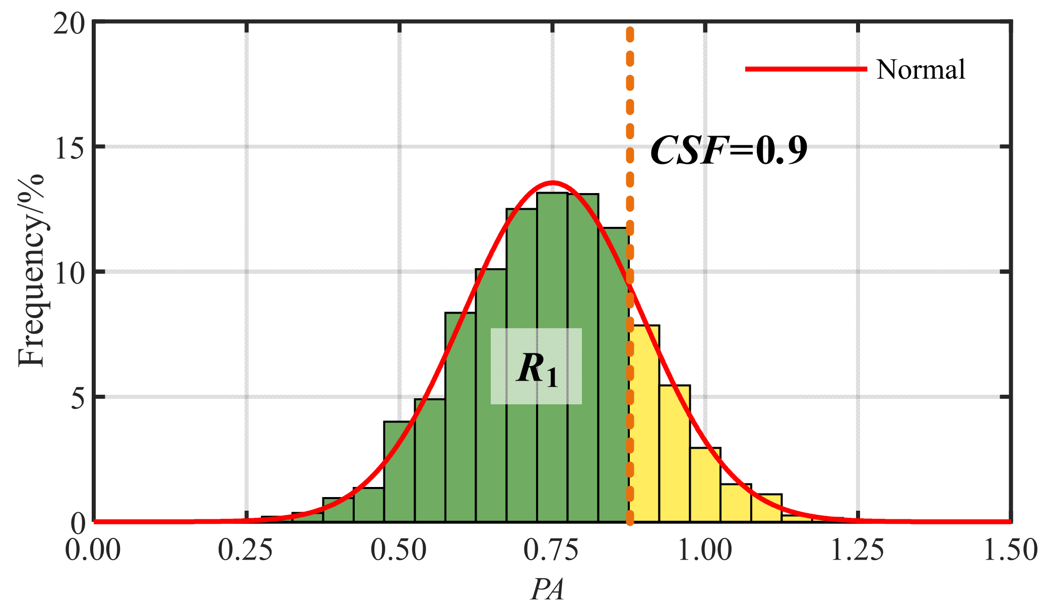
Obviously, the CSF formula Equation (11) is very similar to the PA formula presented in Equation (1). Indeed, CSF represents a critical threshold for PA, and it is considered that when PA does not exceed CSF, the P_pre calculated by FAM is of practical significance. This is because, for a specific set of PA from FAM, a smaller PA implies a smaller P_pre with P_exp being certain, while using a smaller P_pre to guide structural design is conservative and safe. Therefore, the determination of CSF is closely related to the confidence level (R₁) of FAM prediction [31], and their relationships are shown in Equations (14) and (15) and Figure 2. It is clear that CSF represents the upper bound of the most PA values for a FAM when R₁ is close to 1, and this paper suggests CSF falling within the range where R₁ is set at [80.000%, 99.999%], i.e., $\left[CS{F}_{R_1=80.000\%}, CS{F}_{R_1=99.999\%}\right]$.

$$R_1=Pr\left(PA\le CSF\right)={\displaystyle \underset{0}{\overset{CSF}{\int }}PDF(PA)\mathrm{d}PA},$$

(14)

$$CSF=PD{F}^{-1}(R_1),$$

(15)

where Pr(•) is the probability; PDF(•) is the Probability Density Function; PDF⁻¹(•) is the inverse function of PDF.

Notably, CSF can be for comparison with the Safety Factor (SF) calculated by Equation (16) in design to assess structural safety. This assessment method argues that when SF exceeds CSF, which is equivalent to P_op being less than P_exp, the structure is safe. The derivation process is shown in Equation (17), which excludes the influence of predicted values.

$$SF={\displaystyle \frac{P_{\mathrm{rpre}}}{P_{\mathrm{op}}}},$$

(16)

$$Pr(SF>CSF)=Pr({\displaystyle \frac{P_{\mathrm{rpre}}}{P_{\mathrm{op}}}}>{\displaystyle \frac{P_{\mathrm{rpre}}}{P_{\exp }}})=Pr({\displaystyle \frac{1}{P_{\mathrm{op}}}}>{\displaystyle \frac{1}{P_{\exp }}})=Pr(P_{\mathrm{op}}<P_{\exp }),$$

(17)

where P_rpre is the recommended predicted pressure in design; P_op is the operational pressure; Pr(•) is the probability.

Ideally, P_pre should always equal P_exp, with the corresponding CSF being 1. In this case, the structure is regarded as safe when SF exceeds 1, and unsafe otherwise. However, due to potential prediction errors in FAM, P_pre usually does not equal P_exp. If the P_rpre used for design is less than P_exp, i.e., CSF is less than 1, it is considered that the structure fails when SF is less than 1, while P_op has not yet reached P_exp at this time. This design tends to be conservative. Conversely, if CSF is larger than 1, it is assumed that SF exceeds 1 and the structure may not yet be damaged. However, in practice, when SF exceeds 1, P_op has already surpassed P_pre, making the design risky. Therefore, to ensure the safety requirement of structural reliability assessment, the ideal CSF value should preferably not exceed 1. Considering the constraints imposed by the R₁ of FAM prediction, this paper argues that at least $CS{F}_{R_1=80.000\%}$ should be guaranteed not to exceed 1, ensuring basic 80% safety level for structural reliability assessment. It is evident that after scaling the original PA using CSF with Equation (13), PA’ necessarily satisfies the requirement that $CS{F_{R_1=80.000\%}}^{\prime }$ is no more than 1, indicating the rationality and reliability of the optimization procedure in mechanism.

4.2. Flowchart

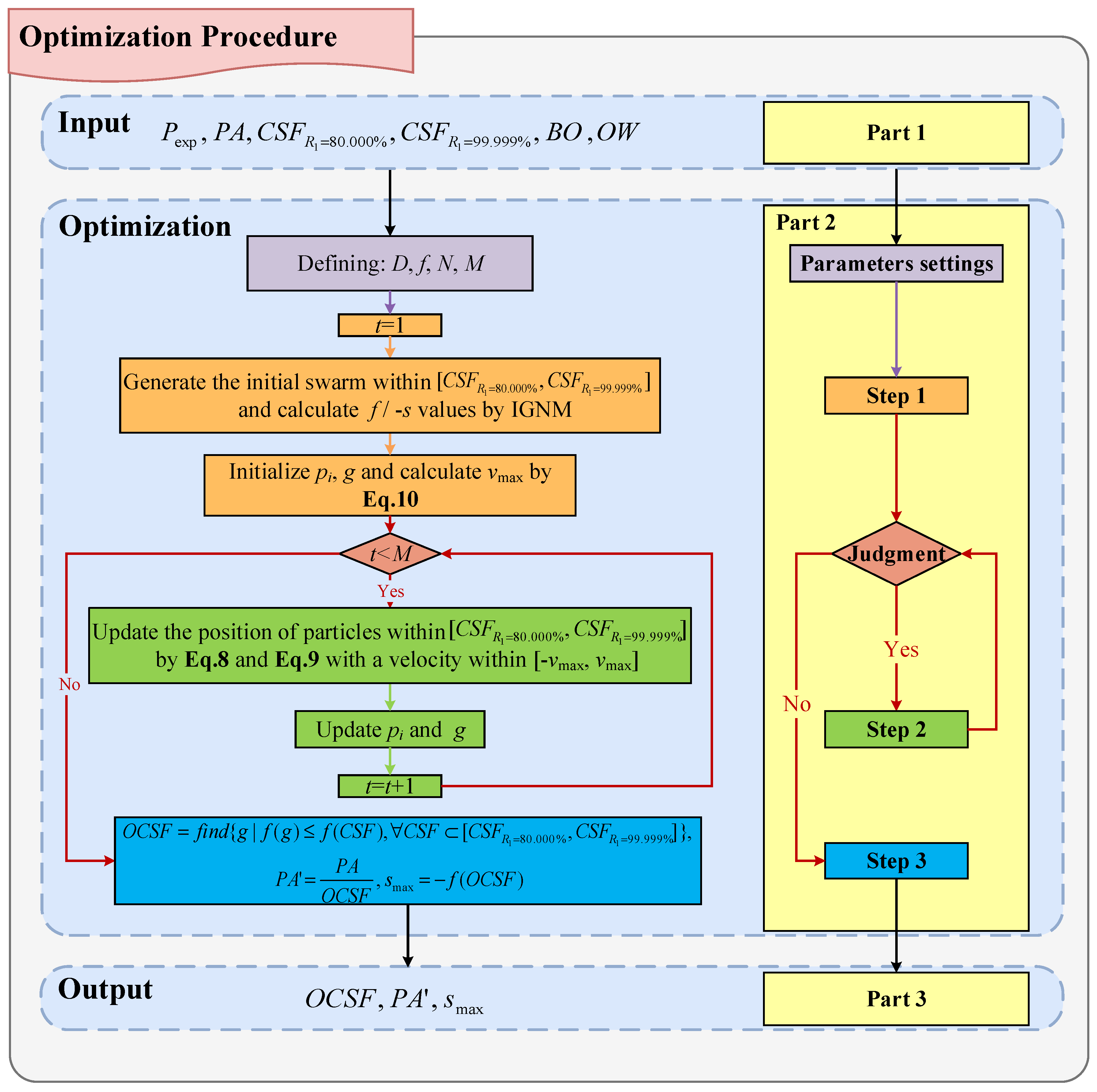
The optimization procedure can be constructed based on basic definitions, which can be divided into three parts: input, optimization and output, as shown in Figure 3.

(1)

Part 1: Input. Input parameters cover six elements, including the experimental pressure (P_exp), FAM’s Prediction Accuracy (PA), minimum and maximum CSF values ($CS{F}_{R_1=80.000\%} \mathrm{and} CS{F}_{R_1=99.999\%}$) and relative importance degrees among different indicators in EIS (BO and OW). Specifically, PA is calculated by Equation (1) where the P_pre values are determined by FAMs. $CS{F}_{R_1=80.000\%} \mathrm{and} CS{F}_{R_1=99.999\%}$ are suggested by the values corresponding to FAM’s confidence level (R₁) equaling to 80.000% and 99.999%, respectively. BO and OW are determined by users’ needs.

(2)

Part 2: Optimization. The optimization is carried out by PSO. Four optimization parameters are still required before iteration, including the dimension of particles (D), fitness (f), particles number (N) and the maximum number of iterations (M), as shown in purple box of part 2 in Figure 3. Specifically, D is defined as 1, since the particle is defined as an individual element CSF in the optimization procedure. f defined as −s, is calculated with IGNM. N and M’s default settings are 50 and 50, respectively, which can be adjusted by users’ needs. Next, the optimization process is divided into the following three steps, as shown in part 2 of Figure 3.

• Step 1: Initialization. The part covers three sub-steps as indicated in the orange boxes in part 2 of Figure 3. Firstly, the number of iterations t is set as 1. Then, the procedure generates the initial swarm within $[CS{F}_{R_1=80.000\%}, CS{F}_{R_1=99.999\%}]$ and calculates f, i.e., −s by IGNM. Finally, it initializes the local optimal particle p_i of individual particle and the global optimal particle g of the swarm. Here, p_i equals the particle’s own initial value. g is determined by the position of the minimum f value in the swarm. In addition, the maximum speed of particles v_max is determined by Equation (10).
• Step 2: Iteration. When the judgment condition (t is less than the maximum number of iterations M) is satisfied, the iteration is carried out, as shown in the pink area at part 2 of Figure 3. Iteration covers three sub-steps as indicated in the green boxes in part 2 of Figure 3. Firstly, the positions of particles are updated by Equations (8) and (9) in $[CS{F}_{R_1=80.000\%}, CS{F}_{R_1=99.999\%}]$ by a velocity in [−v_max, v_max]. Then, update the positions of p_i and g corresponding to the latest minimum f value by that specific individual and the swarm, respectively. Finally, update t with t + 1 for next iteration.
• Step 3: Calculation. When this judgment condition (t is less than the maximum number of iterations M) is not satisfied, the calculation begins. Calculation includes three aspects as presented in a blue box in part 2 of Figure 3. Firstly, the optimal CSF (OCSF) is calculated, which equals to g value at the last iteration, i.e., the found CSF value corresponding to the minimum f value in $[CS{F}_{R_1=80.000\%}, CS{F}_{R_1=99.999\%}]$. The second one is PA’ which is the ratio of the original input PA to OCSF calculated by Equation (13) and the last one is the maximum s_max, i.e., −f(OCSF).

(3)

Part 3: Output. Output includes 3 parameters: OCSF, PA’ and s_max.

5. Empirical Verification

To exhibit the validity and advantages of the procedure in improving FAM’s Prediction Performance (PP), BS 7910:2019 (short in BS7910 in this paper) and CorLAS were used as two examples for optimization, whose computational theories could be found in Reference [12]. To conduct the optimization, six input parameters presented in Section 4.2 were set as follows.

The P_exp values used here were collected based on 250 full-scale burst tests on cracked pipes [32,33,34,35,36,37,38,39,40,41,42], with specific data provided in Reference [12]. Considering the limited applicability of different FAMs, the number of test data sets available for BS7910 and CorLAS is 239 and 245, respectively. The calculated original Prediction Accuracy (PA) values were calculated with FAMs’ P_pre and the P_exp database by Equation (1). As for $[CS{F}_{R_1=80.000\%}, CS{F}_{R_1=99.999\%}]$ limited by the confidence level (R₁) of FAM prediction, the ranges for BS7910 and CorLAS were set as [0.48, 1.04] and [1.22, 2.63], respectively [31]. BO and OW between (C₁, C₂, C₃, C₄, C₅, C₆, C₇) varied depending on the analysis objective and the initial values adopted for optimization were set as (1, 2, 2, 3, 4, 7, 9) and (9, 8, 8, 7, 6, 3, 1), respectively.

5.1. Rationality of Fitness Setting

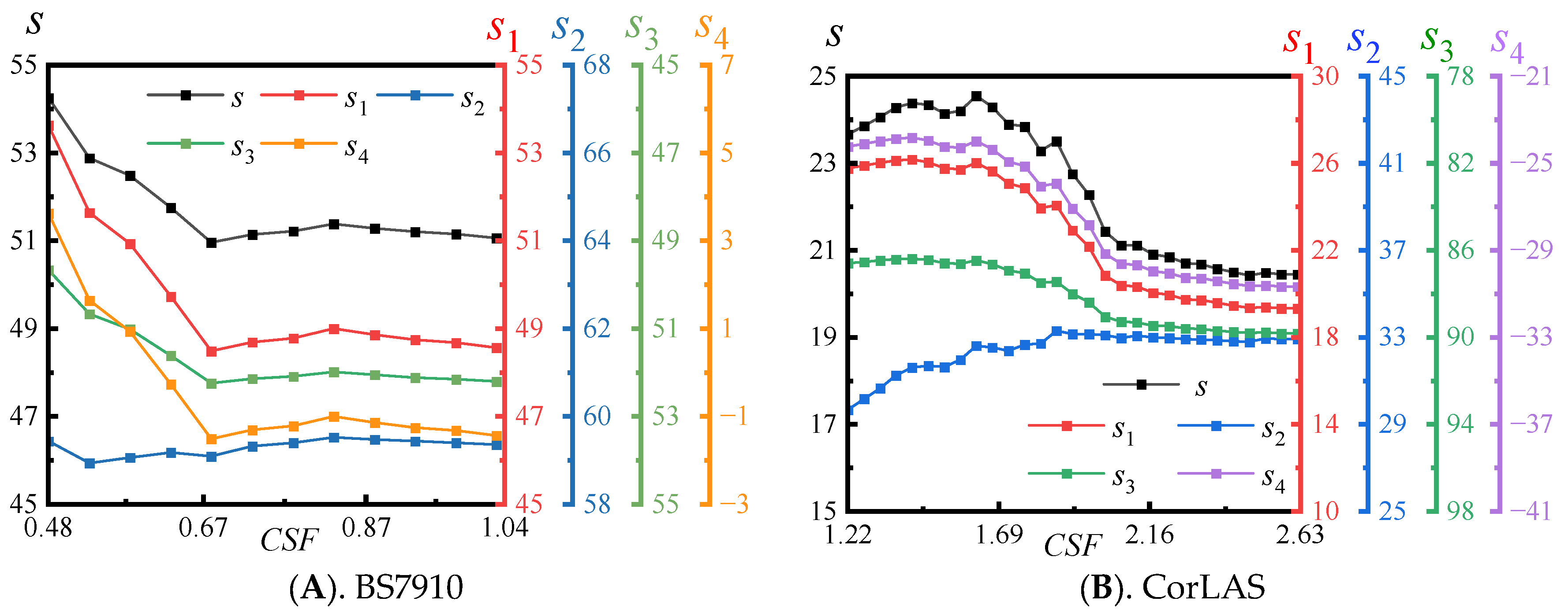
The rationality of fitness (f) setting for the optimization procedure is mainly reflected in the convexity of f-function. Therefore, BS7910 and CorLAS have been first employed to explore whether there is a unique solution during optimization process by analyzing the relationship between CSF and f values with initial parameter settings. Notably, CSF values were taken at 0.05 intervals within specific $[CS{F}_{R_1=80.000\%}, CS{F}_{R_1=99.999\%}]$. f has been defined as the opposite of IGNM’s score (−s). In order to facilitate the demonstration, s was directly used for the convexity analysis here, which could be computed with the original P_exp and the modified Prediction Accuracy (PA’) by IGNM. Given the above assumptions, the relationships between CSF and s for BS7910 and CorLAS were presented in Figure 4. Note that the scores (s₁, s₂, s₃, s₄) computed by GNM have also been included to demonstrate the superiority of the IGNM-based f setting. Except for s₃, higher scores (s, s₁, s₂, s₄) indicate enhancer PP of FAMs.

From Figure 4, it is evident that there is a unique max s in each sub-figure, signifying that the fitness function is convex to CSF no matter for BS7910 or CorLAS. Specifically, BS7910’s s sharply declines with CSF’s increase, followed by a slight variation with the CSF over 0.67, reaching its only maximum around the minimum CSF, i.e., CSF = 0.48. This trend is consistent with s₁, s₄ and −s₃, whose values are positively correlated with PP. Notably, s₂ varies slightly with CSF’s change, indicating a poor sensitivity to CSF. This demonstrates the shortcoming of single decision-making model scoring, which may lead to ineffective optimization. In contrast, s is more suitable for PP’s comprehensive optimization, which integrates the primary characteristics of various decision-making models. As for CorLAS, its s increases slightly and then decreases with the increase in CSF, peaking near CSF = 1.60. The other scores here showcase this similar pattern, except that s₂ continuously increases at a decreasing rate. This indicates that s exhibits most of the variability in sub-scores, thereby mitigating the risk of single-method bias.

In summary, the results above illustrate the convexity of the fitness function based on IGNM, ensuring the uniqueness of the optimization solution. More importantly, not only can the fitness mitigate the potential biases and limitations of a single decision-making model to some extent, improving the accuracy and generalization ability of PP’s overall evaluation, but it can also fully integrate the characteristics of various decision-making models, thereby enhancing the comprehensiveness and robustness of the subsequent optimization. These findings further validate the feasibility of the IGNM’s arithmetic averaging integration method, as well as the rationality and advantages of the optimization procedure proposed in this study.

5.2. Optimization Effect

To prove the validity of the procedure, the optimization effects for BS7910 and CorLAS under the initial parameter settings were both presented in two aspects: FAMs’ PP scores and their PA distribution.

5.2.1. PP Scores

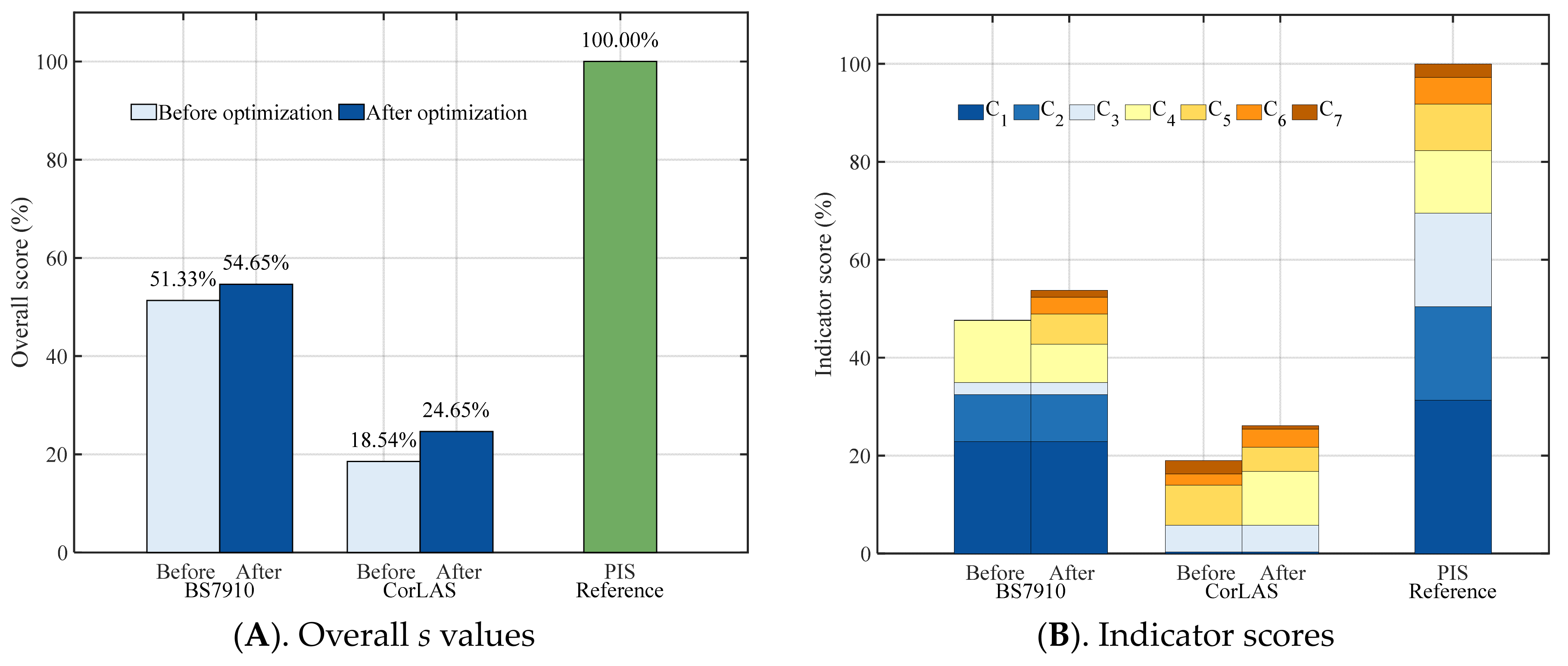
After optimization, the changes in PP’s overall score s calculated by IGNM for BS7910 and CorLAS are presented in Figure 5A. Furthermore, to analyze the optimization’s influences on the multi-dimensional characteristics of PP, the scores of indicators within Evaluation Indicator System (EIS) before and after optimization calculated by SWM were presented in Figure 5B. Here, SWM provided intuitive absolute scores directly correlated with indicator changes, enabling the comparison of each indicator’s sensitivity to optimization.

From Figure 5A, it is clear that s values optimized appear to increase for both BS7910 and CorLAS, proving the validity of the procedure. Specifically, s values of BS7910 and CorLAS are effectively improved from 51.33% to 54.65% with up to 3.32% increase and 18.54% to 24.65% with up to 6.09% increase, respectively.

Moreover, as shown in Figure 5B, the total indicator scores of the two optimized FAMs, i.e., the s₁ values calculated by SWM, also exhibit improvements consistent with the overall s, which can be confirmed by the fact that s and s₁ exhibit nearly identical variation characteristics with CSF changes, as presented in Figure 4. Specifically, the stability indicators’ scores for both models, including correlation C₁, multi-modality C₂ and dispersion C₃, show no variation. Meanwhile, the scores of DLCs comprising risk C₄, conservatism C₅, robustness C₆ and accuracy C₇ exhibit distinct significant changes. For BS7910, the scores of C₅, C₆ and C₇ have noticeably increased, while the score of C₄ has decreased. As for CorLAS, C₄ and C₆ scores show significant increases, while C₇ and C₅ scores exhibit decreases. Notably, although the specific score changes in DLCs differ for different FAMs, the total values have been raised. In addition, the changes in C₄ and C₅ scores for both models are more significant than those in C₆ and C₇. This is related to the higher importance of C₄ and C₅ when setting the relative degrees BO and OW for Best-Worst Method (BWM), resulting in their larger weights compared to C₆ and C₇. Hence, C₄ and C₅ contribute more to the changes in PP scores.

In summary, the changes in PP scores initially reveal that the procedure achieves overall performance enhancement by modifying DLCs whose influences on scoring are associated with parameter settings, while not changing the stability. This may be related to the way in which the independent variable CSF optimizes PP, i.e., overall scaling PA values, which could not alter the numerical values of correlation C₁, multi-modality C₂ and dispersion C₃ from a mathematical perspective.

5.2.2. PA Distribution

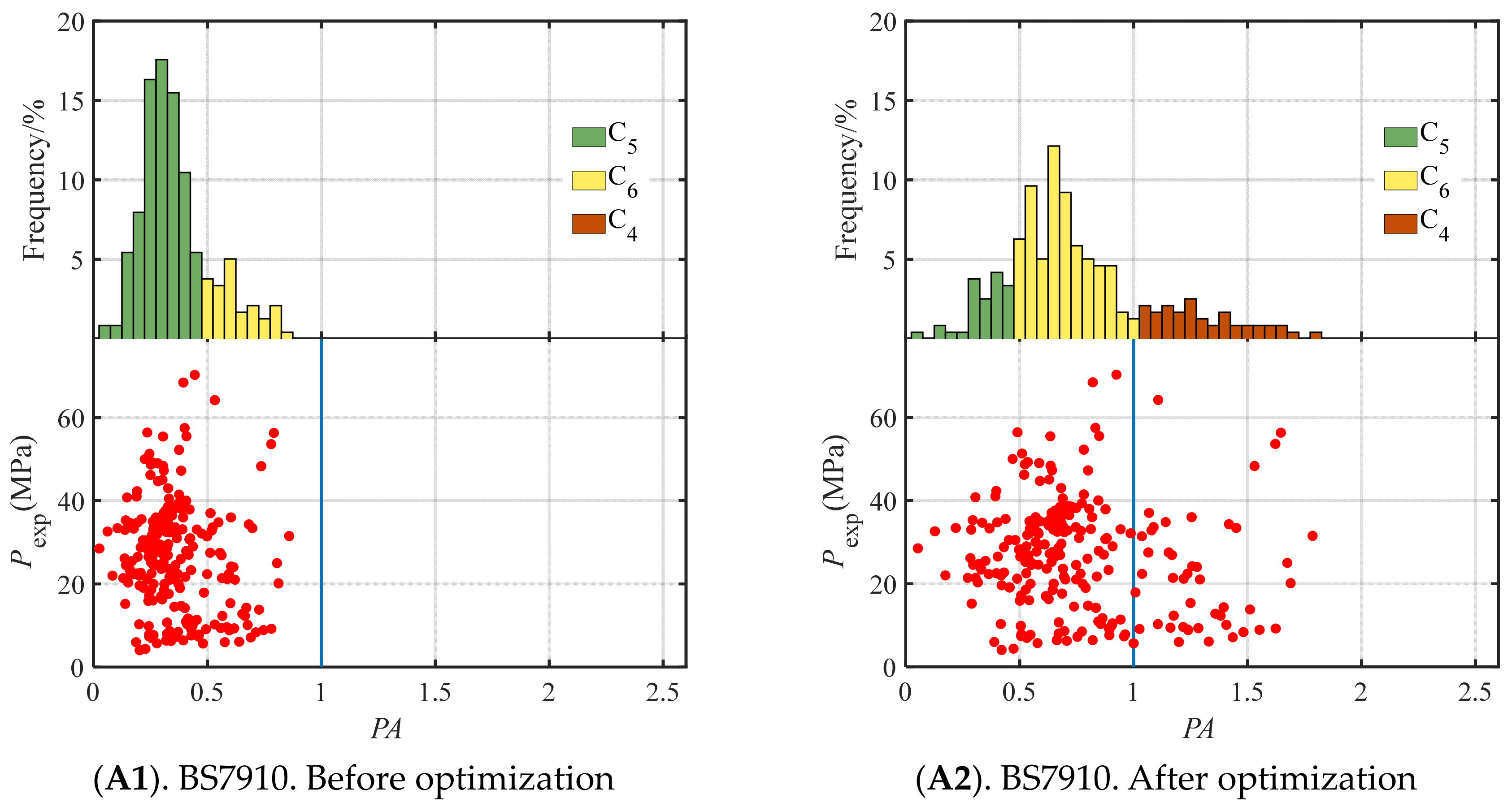
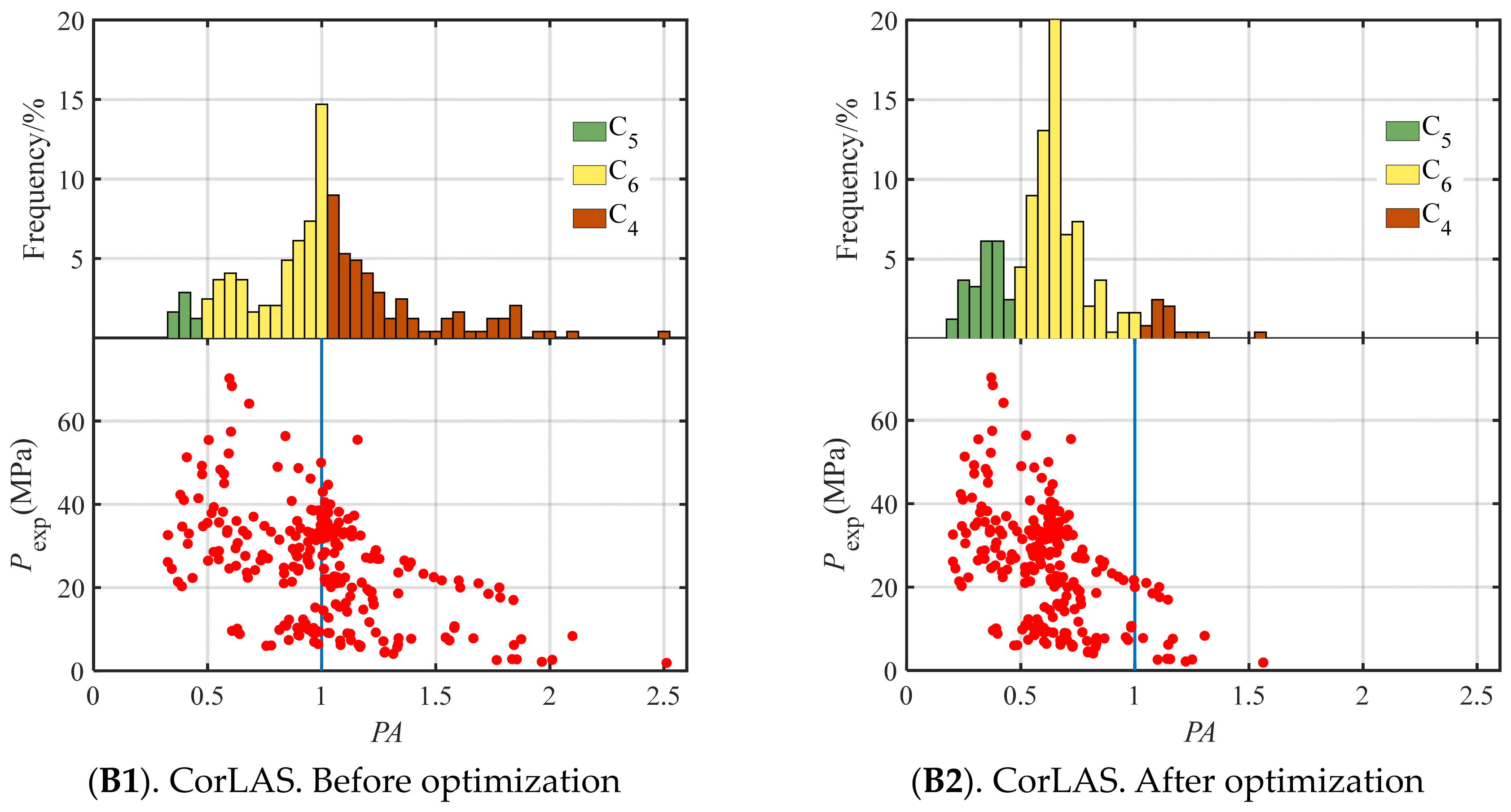
The PA distributions of BS7910 and CorLAS have changed significantly before and after the optimization as visualized in Figure 6.

From Figure 6, the optimized PA values distribute more evenly across the conservatism C₅, robustness C₆ and risk C₄. Both the over conservatism of BS7910’s PP and the high risk of CorLAS’s PP have been corrected, demonstrating greater balance compared to the stage before optimization. As for the value of accuracy C₇, it may decrease or increase depending on whether the overall distribution is closer to or farther from 1.

Specifically, for BS7910, PA values overall bias to the right because the optimal CSF (OCSF) found is 0.4809 less than 1 and the modification for PA by Equation (13) enlarges the values. Corresponding to the DLCs, the percentage of C₅ has decreased, while that of C₄ and C₆ has increased after the optimization. In addition, accuracy C₇ value has decreased since the originally conservative results are scaled up to around 1. Moreover, considering C₄, C₅ and C₇ are cost indicators and C₆ is a benefit indicator, the changes in C₅, C₆ and C₇ are beneficial to the improvement of BS7910’s PP, which can correspond to the increases in indicators’ scores presented in Figure 5B. Meanwhile, although the increased C₄ brings a deduction for the overall performance based on its weight calculated by BWM, the overall PP has still been improved by accommodating comprehensive characteristics. Furthermore, the OCSF of BS7910 at 0.4809 is very close to the lower bound of the CSF search range at 0.4800. This is primarily because the model’s original PA values are overly conservative, as shown in Figure 6(A1), leaving significant room for improvement in the corresponding C₅ score. The procedure tends to output larger and more balanced PA’ with Equation (13), resulting in a smaller OCSF that approaches the lower bound.

As for CorLAS, the output OCSF is 1.6071 larger than 1, resulting in an overall reduction in PA values, which differs from BS7910. This is mainly caused by the fact that CorLAS’s PP has a high-risk level, and the performance improvement is achieved by decreasing C₄ while increasing C₆. However, this modification process also involves unfavorable changes, including the increases in C₅ and C₇. Nevertheless, the final comprehensive PP is still significantly enhanced.

In summary, the optimization procedure has been proven to enhance FAM’s PP and the improvement is achieved by modifying the DLCs of PA. Notably, the changes in C₄, C₅, C₆ and C₇ during the optimization process often create different effects on the overall PP score. While the preferences for specific indicators can be adjusted through parameter settings, enabling the procedure to suit various application requirements. In addition, the OCSF values obtained for both models through PSO correspond well with the peak values of overall s shown in Figure 4, sufficiently demonstrating the effectiveness of PSO and the validity of the optimization procedure.

5.3. Tests on Application Preferences

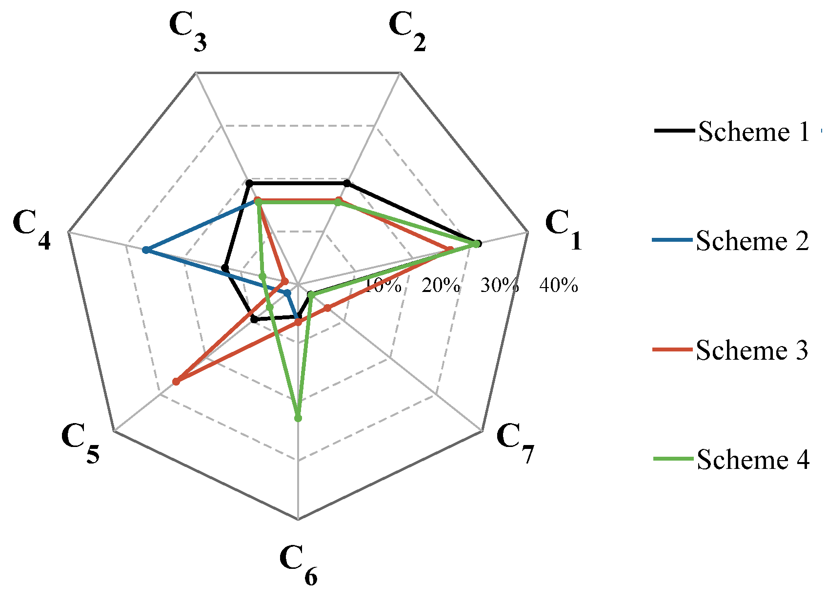
To further exhibit the generalization capability of the optimization procedure, this section introduced three additional schemes which differed in their FAM application preferences for high conservatism, high risk and high robustness, respectively. The optimization tests were conducted for CorLAS and the four parameter settings, together with the initial optimization Scheme 1 discussed in Section 5.1 and Section 5.2, were summarized in

Table 1. Different settings of indicators’ relative importance degrees.

Scheme	BO (C1, C2, C3, C4, C5, C6, C7)	OW (C1, C2, C3, C4, C5, C6, C7)
Scheme 1-Initial	(1, 2, 2, 3, 4, 7, 9)	(9, 8, 8, 7, 6, 3, 1)
Scheme 2-Conservatism	(1, 2, 2, 1, 9, 5, 5)	(9, 8, 8, 9, 1, 5, 5)
Scheme 3-Risk	(1, 2, 2, 9, 1, 5, 5)	(9, 8, 8, 1, 9, 5, 5)
Scheme 4-Robustness	(1, 2, 2, 5, 5, 1, 5)	(9, 8, 8, 5, 5, 9, 5)

. Specifically, the newly added Scheme 2 preferred prediction results with high conservatism by reducing the importance of conservatism C5 and increasing that of risk C4. Scheme 3 prioritized high risky prediction results, which was achieved through the opposite operations of Scheme 2. Scheme 4 preferred high robustness, which was performed by increasing the importance of C6. Here, the added schemes set the importance of non-preferred DLCs to the intermediate value of 5, while keeping the stability unchanged relative to Scheme 1. Based on these assumptions, the weights of each scheme’s indicators calculated by BWM were shown in Figure 7.

From Figure 7, it is evident that compared to the initial Scheme 1, each added scheme significantly increases the weight of its high-importance indicator. Notably, Schemes 2 and 3 also significantly reduce the weights of low-importance indicators at the same time. Hence, compared to Scheme 4, which assigns non-preferred DLCs intermediate importance levels, Schemes 2 and 3 exhibit more significant reductions in the weights of C5 and C4, respectively, relative to the original Scheme 1, thereby better emphasizing overall performance preferences.

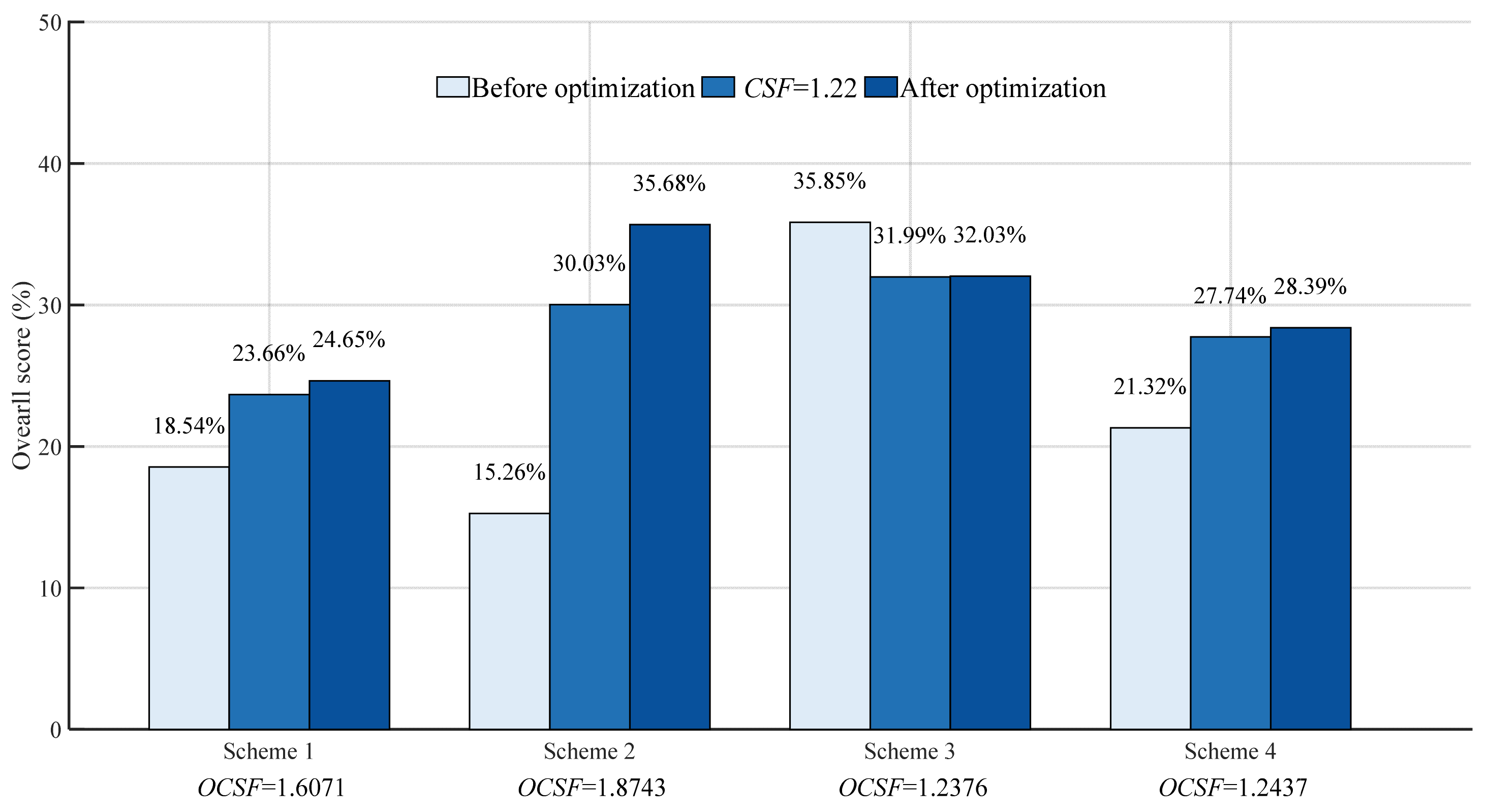
After the procedure optimization, the OCSF found for each scheme and the changes in the overall s values calculated by IGNM were presented in Figure 8. Notably, Figure 8 not only presents the PA scores before and after optimization, but also introduces an additional score corresponding to the case where the independent variable CSF is taken as $CS{F}_{R_1=80.000\%}$, which can guarantee that the $CS{F_{R_1=80.000\%}}^{\prime }$ of the optimized PA’ is no more than 1. This is related to the previously mentioned CSF range for CorLAS, limited by R₁, which was set as [1.22, 2.63]. Obviously, the initial PA of CorLAS, corresponding to CSF equal to 1 and less than 1.22, fails to meet the basic safety requirement for structural reliability assessment, i.e., guaranteeing that at least 80% of the predicted results from FAM bias towards safety in design. As shown in Figure 6(B1), CorLAS’s initial PA distribution is mostly risk-biased, failing to achieve the requirement that at least 80% of PA values fall within 1, while the CSF set by the optimization procedure is mechanically capable of ensuring that the optimized prediction results satisfy the basic safety requirement for design as presented in Section 4.1.2. Hence the functionality of the optimization procedure can actually be subdivided into two aspects: guaranteeing basic safety requirement and improving PP scores. Therefore, to align with the needs of practical application, this section also presents the PP scores corresponding to CSF taken as 1.22 for simultaneous references.

As shown in Figure 8, each added preference scheme has found its own OCSF distinct from the initial scheme and exhibits different changes in scores. Specifically, for Scheme 2, its OCSF, 1.8743, is larger than that of Scheme 1, i.e., 1.6071. This is mainly because Scheme 2 tends to produce more conservative prediction results, while the larger OCSF exerts a stronger reduction effect when modifying P_pre with Equation (12). In terms of the optimization mechanism, parameter adjustments in Scheme 2 reduce the weight of C₅ and increase that of C₄, thereby weakening the effect of C₅’s increased proportion on lowering the PP score and enhancing the score improvement effect from C₄’s decreased proportion. These effects enable the optimization to prefer a smaller PA’ distribution when balancing DLCs. As for the overall s improvement, Scheme 2 demonstrates a more significant PP optimization effect compared to Scheme 1. On one hand, this is because the revised weights of indicators tend to amplify the scoring contribution of cost indicator C₄, resulting in a lower initial score for the original over-risk prediction results. On the other hand, the simultaneous adjustments for C₄ and C₅ have deepened the procedure’s optimization degree to some extent.

For Scheme 3, its OCSF, 1.2376, is noticeably lower than that of Schemes 1 and 2. Similarly, this mainly stems from Scheme 3’s preference for high risk, which tends toward larger P_pre, naturally leading to the search of a smaller CSF for adjustment. However, different from Scheme 2 which further optimized PP relative to Scheme 1, Scheme 3’s score optimized even decreased compared to the original score. This is due to Scheme 3’s pursuit of high risk excessively raising the score of the original PP. While from the application perspective, the basic safety of design guidance from the prediction results should be ensured first, and then the scope for optimization could be considered. Thus, the ‘initial score’, now used to assess whether PP has been improved, should be the score 31.99%, corresponding to CSF taken as 1.22, not the original 35.85%, and the procedure still accomplishes the PP improvement task for Scheme 3.

As for Scheme 4, its OCSF is also relatively small for the preference of robustness concentrating most PA within [0.5, 1]. Although the original PA distribution as shown in Figure 6(B1) contains many risky points, its highest frequency cluster lies near 1. Therefore, a CSF value slightly above 1 can achieve both data concentration and bring the densely distributed region into the robustness range. In addition, it is evident that the robustness preference requires less adjustment intensity for prediction results. Reflected in score optimization, the procedure’s enhancement effect for Scheme 4 is weaker than that for Scheme 2, while similar to that for the initial Scheme 1 with no distinct preferences.

In summary, the optimization procedure has been proven to be adaptable to various application preference situations, demonstrating excellent adaptability. By adjusting the importance degrees of specific indicators, the PP’s emphasis of them and sensitivity to their changes can be altered, thereby achieving the goal of promoting or suppressing specific performance aspects. Notably, although preference settings may be too extreme in some cases, the optimization procedure still ensures that the output results can meet the basic safety requirement for design, further demonstrating the reliability and engineering value of the procedure.

6. Discussion

The optimization procedure based on Improved Guo-Ni Model (IGNM) and Particle Swarm Optimization (PSO) proposed in this paper has been proven to effectively increase the overall Prediction Performance (PP) of FAM by balancing Distributional Location Characterizations (DLCs) in case applications. Notably, the optimization for the overall PP score s essentially reflects an aggregate improvement through incorporating the variations in four indicators, including risk (C₄), conservatism (C₅), robustness (C₆) and accuracy (C₇). This means the practical value of the procedure lies not only in the increase in s values, but more significantly in its adjustment and balancing of DLCs. For instance, although BS7910 shows a seemingly modest s improvement of 3.32% under the initial optimization parameters, this net gain results from substantial increases in C₅, C₆ and C₇ scores, which offset the reduction in C₄. When examining the changes in indicator scores, the increases are actually obvious (as shown in Figure 5B). Furthermore, the procedure allows users to adjust their application preferences through parameter settings, enabling flexible modifications for the PA distribution range to suit different engineering requirements. However, despite the procedure’s generalization capability and practical value, several inherent limitations remain to be addressed in future work.

Firstly, the procedure essentially applies linear scaling to the Prediction Accuracy (PA) via a single factor Critical Safety Factor (CSF), which mathematically fails to alter FAM’s inherent cognitive uncertainty related to data structure and PA distribution pattern. Consequently, the optimization could not enhance FAM’s stability indicators, including correlation (C₁), multi-modality (C₂) and dispersion (C₃). This limitation constrained the depth of optimization, and subsequent research could incorporate factors related to the intrinsic properties of FAM itself as independent variables, such as the key calculation parameters for the predicted result P_pre and the selection of computational methods. Enriching the dimensions of candidate solutions could enable the non-linear adjustment of the PA and allow the fundamental optimization for FAM’s inherent characteristics.

Secondly, while the optimization procedure can flexibly adjust FAM’s prediction results according to user preferences regarding DLCs, the overall PA offset always fails to make all modified PA’ values less than 1 when balancing various indicators. Future work could consider integrating physical constraints into the optimization process, such as adding a risk penalty term to the objective function or limiting the range of PA’ in deterministic form. Notably, the constraints should ideally be combined with the previously mentioned non-linear PA correction which is achieved by introducing additional independent variables. This makes it possible for the final optimized PA’ values to be entirely less than 1 while not being excessively conservative, thereby ensuring that the output results fully satisfy the safety requirement for structural reliability assessment in design.

Thirdly, although PSO demonstrates high adaptability for the specific one-dimensional optimization task of this paper, for future work that could increase the dimension of candidate solutions, it may be preferred to compare the performance of PSO with novel intelligent optimization algorithms better suited to high-dimensional optimization, such as Sailfish Optimization (SFO) and Moth-Flame Optimization (MFO), and select the most appropriate optimization tool.

Finally, the optimization procedure has adopted a static optimization framework in the application cases, that is, all the optimal CSFs (OCSFs) are calculated based on a fixed historical experimental dataset to calibrate the model performance. However, in practical engineering, data evolve continuously. Real-time updates of the test sets and corresponding prediction information in the procedure input part may affect the evaluation and adjustment of FAM’s PP. Thus, in order to increase the robustness of the procedure in practical applications, subsequent work could consider periodically re-executing the optimization process based on new datasets or setting up a re-optimization triggering mechanism based on the deviation significance of overall score s or the basic indicators’ scores.

Acknowledging these limitations does not diminish the contributions of this research. Rather, it serves to clearly delineate its application boundaries and chart a path for future studies.

7. Conclusions

In this paper, an optimization procedure for improving the Prediction Performance (PP) of FAM is presented. The procedure is established based on Improved Guo-Ni Model (IGNM) and Particle Swarm Optimization (PSO). IGNM is raised to set fitness for optimization, which can provide an absolute score s for fully quantifying FAM’s PP in terms of the indicators in Evaluation Indicator System (EIS), including stability and Distributional Location Characterizations (DLCs) of FAM’s prediction results. PSO builds an iterative framework for optimization consisting of candidate solutions and fitness. Considering that the s values can be affected by the Critical Safety Factor (CSF), the comprehensive optimization for PP across multiple dimensions can be achieved through searching for the optimal CSF (OCSF), i.e., maximizing s. The conclusions are as follows:

(1)

The convexity tests conducted for the fitness functions of BS7910 and CorLAS demonstrate that the IGNM-based fitness can not only successfully avoid the problem of ineffective optimization targeting a single decision-making model, but also effectively integrate the characteristics of various decision-making models for enhancing the comprehensiveness and robustness of the subsequent optimization. These findings validate the rationality and advantages of the optimization procedure.

(2)

Based on the procedure, BS7910 and CorLAS have been optimized with a set of initial parameters showing no significant preference for DLCs. The results indicated that, for PP’s overall scores, there is an s value improvement up to 3.32% for BS7910 and CorLAS’s s is also effectively improved with up to 6.09% increase, proving the validity of the procedure. For the specific scores in EIS, the scores for DLCs including risk C₄, conservatism C₅, robustness C₆ and accuracy C₇ have significantly changed, while stability shows no variation, revealing that the procedure achieves overall performance enhancement by modifying DLCs. As for Prediction Accuracy (PA) distribution, the optimized PA values of both FAMs show better balance for DLCs.

(3)

Three added application preference optimization tests conducted for CorLAS indicate that the optimization results can satisfy different prediction preferences which can be adjusted by modifying the relative importance degrees of DLCs, demonstrating the procedure’s excellent generalization capability. Furthermore, it is noteworthy that the procedure can guarantee that the output results always meet the basic safety requirement for design of the mechanism, further proving the reliability and engineering value of the procedure.

(4)

The optimization procedure has been proven to effectively increase the PP of FAM by balancing DLCs, providing a new idea for the optimization control of FAM’s overall performance, i.e., utilizing a comprehensive evaluation model to set the goal about PP optimization. While the procedure has failed to change the stability of FAM prediction by scaling PA with CSF. The future research will continue to explore incorporating additional factors influencing the PA and other algorithms better suited to multidimensional optimization. Enriching the candidate solution dimensions enables non-linear adjustment of PA, thereby fundamentally optimizing the inherent characteristics of FAM. Furthermore, adding some physical constraints during the optimization process may allow the final optimized PA values to be fully less than 1 without being overly conservative, thus ensuring the output results fully meet the safety requirements for structural reliability assessment in the design. Additionally, considering the real-time nature of the input data, periodic optimization can be considered to enhance the procedure robustness.

References

1. Guo, L.; Zhou, J.; Dai, Y. Time-dependent failure probability analysis of corroded pipelines based on different stochastic degradation processes. Acta Pet. Sin. 2019, 40, 1542–1552. (In Chinese) [Google Scholar]
2. Shuai, Y.; Zhang, Y.; Shuai, J.; Xie, D.; Zhu, X.; Zhang, Z. A novel framework for predicting the burst pressure of energy pipelines with clustered corrosion defects. Thin-Walled Struct. Part A 2024, 205, 112413. [Google Scholar] [CrossRef]
3. Okodi, A.; Lin, M.; Yoosef-Ghodsi, N.; Kainat, M.; Hassanien, S.; Adeeb, S. Crack propagation and burst pressure of longitudinally cracked pipelines using extended finite element method. Int. J. Press. Vessel. Pip. 2020, 184, 104115. [Google Scholar] [CrossRef]
4. Vishnuvardhan, S.; Murthy, A.R.; Choudhary, A. A review on pipeline failures, defects in pipelines and their assessment and fatigue life prediction methods. Int. J. Press. Vessel. Pip. 2023, 201, 104853. [Google Scholar] [CrossRef]
5. Gong, C.; Guo, S.; Zhang, R.; Frangopol, D.M. Prediction of burst pressure of corroded thin-walled pipeline elbows subjected to internal pressure. Thin-Walled Struct. 2024, 199, 111861. [Google Scholar] [CrossRef]
6. GB/T 19624-2019; Safety Assessment for in-Service Pressure Vessels Containing Defects. China Standards Press: Beijing, China, 2019. (In Chinese)
7. BS 7910:2019; Guide to Methods for Assessing the Acceptability of Flaws in Metallic Structures. British Standards Institution: London, UK, 2019.
8. Yan, Z.; Zhang, S.; Zhou, W. Model error assessment of burst capacity models for energy pipelines containing surface cracks. Int. J. Press. Vessel. Pip. 2014, 120-121, 80–92. [Google Scholar] [CrossRef]
9. Zhang, X.; Zheng, Q.; Leung, J.; Adeeb, S. Reliability-based assessment of cracked pipelines using monte carlo simulation technique with CorLAS™. In Proceedings of the ASME Pressure Vessels and Piping Conference, Las Vegas, NV, USA, 17–22 July 2022; p. V002T03A051. [Google Scholar]
10. Cosham, A.; Hopkins, P.; Leis, B. Crack-like Defects in Pipelines: The Relevance of Pipeline-specific Methods and Standards. In Proceedings of the International Pipeline Conference, Calgary, AB, Canada, 24–28 September 2012. [Google Scholar]
11. Yan, J.; Zhang, S.; Kariyawasam, S.; Pino, M.; Liu, T. Validate Crack Assessment Models with In-Service and Hydrotest Failure. In Proceedings of the International Pipeline Conference, Calgary, AB, Canada, 24–28 September 2018. [Google Scholar]
12. Guo, L.; Niffenegger, M.; Jing, Z. Statistical inference and performance evaluation for failure assessment models of pipeline with external axial surface cracks. Int. J. Press. Vessel. Pip. 2021, 194, 104480. [Google Scholar] [CrossRef]
13. Guo, L.; Niffenegger, M.; Zhou, J. A novel procedure to evaluate the performance of failure assessment models. Reliab. Eng. Syst. Saf. 2022, 226, 108667. [Google Scholar] [CrossRef]
14. Seyedmohammadi, J.; Sarmadian, F.; Jafarzadeh, A.A.; Ghorbani, M.A.; Shahbazi, F. Application of SAW, TOPSIS and fuzzy TOPSIS models in cultivation priority planning for maize, rapeseed and soybean crops. Geoderma 2018, 310, 178–190. [Google Scholar] [CrossRef]
15. Lin, S.-S.; Shen, S.-L.; Zhou, A.; Xu, Y.-S. Novel model for risk identification during karst excavation. Reliab. Eng. Syst. Saf. 2021, 209, 107435. [Google Scholar] [CrossRef]
16. Cristóbal, J.R.S. Multi-criteria decision-making in the selection of a renewable energy project in spain: The Vikor method. Renew. Energy 2011, 36, 498–502. [Google Scholar] [CrossRef]
17. Jia, X.; Wang, X. A PROMETHEE II method based on regret theory under the probabilistic linguistic environment. IEEE Access 2020, 99, 1. [Google Scholar] [CrossRef]
18. Zhang, H.; Dong, S.; Ling, J.; Zhang, L.; Cheang, B. A modified method for the safety factor parameter: The use of big data to improve petroleum pipeline reliability assessment. Reliab. Eng. Syst. Saf. 2020, 198, 106892. [Google Scholar] [CrossRef]
19. Kiswendsida, K.J.; Huang, Q. Probabilistic burst pressure prediction model for pipelines with single crack-like defect. Int. J. Press. Vessel. Pip. 2024, 207, 105084. [Google Scholar]
20. Kiefner, J.F. Modified Ln-Secant equation improves failure prediction. Oil Gas J. 2008, 106, 64–66. [Google Scholar]
21. Su, Y.; Li, J.; Yu, B.; Zhao, Y.; Yao, J. Fast and accurate prediction of failure pressure of oil and gas defective pipelines using the deep learning model. Reliab. Eng. Syst. Saf. 2021, 216, 108016. [Google Scholar] [CrossRef]
22. Sun, H.; Zhou, W. Classification of failure modes of pipelines containing longitudinal surface cracks using mechanics-based and machine learning models. J. Infrastruct. Preserv. Resil. 2023, 4, 5. [Google Scholar] [CrossRef]
23. Ren, M.; Zhang, Y.; Fan, M.; Xiao, Z. Numerical simulation and ANN prediction of crack problems within corrosion defects. Materials 2024, 17, 3237. [Google Scholar] [CrossRef]
24. Huang, M.; Wan, N.; Zhu, H. Reconstruction of structural acceleration response based on CNN-BiGRU with squeeze-and-excitation under environmental temperature effects. J. Civ. Struct. Health Monit. 2025, 15, 985–1003. [Google Scholar] [CrossRef]
25. Sharma, R.; Matharu, J.S.; Parmar, K.S. A survey on Particle Swarm Optimization: Evolution, adaptations and practical implementations. Appl. Soft Comput. 2026, 186, 114016. [Google Scholar] [CrossRef]
26. Huang, M.; Gül, M.; Zhu, H. Vibration-Based Structural Damage Identification under Varying Temperature Effects. J. Aerosp. Eng. 2018, 31. [Google Scholar] [CrossRef]
27. Huang, M.; Ling, Z.; Sun, C.; Lei, Y.; Xiang, C.; Wan, Z.; Gu, J. Two-stage damage identification for bridge bearings based on sailfish optimization and element relative modal strain energy. Struct. Eng. Mech. 2023, 86, 715–730. [Google Scholar]
28. Huang, M.; Li, X.; Lei, Y.; Gu, J. Structural damage identification based on modal frequency strain energy assurance criterion and flexibility using enhanced Moth-Flame optimization. Structures 2020, 28, 1119–1136. [Google Scholar] [CrossRef]
29. Liang, F.; Brunelli, M.; Rezaei, J. Consistency issues in the best worst method: Measurements and thresholds. Omega 2020, 96, 102175. [Google Scholar] [CrossRef]
30. Saaty, T.L. Fundamentals of the analytic network process- dependence and feedback in decision-making with a single network. J. Syst. Sci. Syst. Eng. 2004, 13, 129–157. [Google Scholar] [CrossRef]
31. Guo, L. The Study on Failure Assessment of Defect Pipes; Dalian University of Technology: Dalian, China, 2022. (In Chinese) [Google Scholar]
32. Kiefner, J.F.; Maxey, W.A.; Eiber, R.J.; Duffy, A.R. Failure stress levels of flaws in pressurized cylinders. ASTM Spec. Tech. Publ. 1973, 536, 461–481. [Google Scholar]
33. Hosseini, A.; Cronin, D.; Plumtree, A.; Kania, R. Experimental Testing and Evaluation of Crack Defects in Line Pipe. In Proceedings of the International Pipeline Conference, Calgary, AB, Canada, 27 September–1 October 2010. [Google Scholar]
34. Ruggieri, C.; Dotta, F. Numerical modeling of ductile crack extension in high pressure pipelines with longitudinal flaws. Eng. Struct. 2011, 33, 1423–1438. [Google Scholar] [CrossRef]
35. Mannucci, G.; Demofonti, G. Fracture Properties of API X 100 Gas Pipeline Steels; Europipe: Mülheim an der Ruhr, Germany, 2002. [Google Scholar]
36. Rana, M.D.; Selines, R.J. Structural integrity assurance of high-strength steel gas cylinders using fracture mechanics. Eng. Fract. Mech. 1988, 30, 877–894. [Google Scholar] [CrossRef]
37. Staat, M. Plastic collapse analysis of longitudinally flawed pipes and vessels. Nucl. Eng. Des. 2004, 234, 25–43. [Google Scholar] [CrossRef]
38. Keller, H.P.; Junker, G.; Merker, W. Fracture analysis of surface cracks in cylindrical pressure vessels applying the two-parameter fracture criterion (TPFC). Int. J. Pres. Ves. Pip. 1987, 29, 113–153. [Google Scholar] [CrossRef]
39. Brocks, W.; Kunecke, G.; Wobst, K. Stable crack growth of axial surface flaws in pressure vessels. Int. J. Pres. Ves. Pip. 1989, 40, 77–90. [Google Scholar] [CrossRef]
40. Shuai, J.; Xu, K. Validation of failure assessment curve of linepipe containing cracks. J. Mech. Strength 2003, 25, 251–253. (In Chinese) [Google Scholar]
41. Rana, M.D. Experimental verification of fracture toughness requirement for leak- before-break performance for 155-175ksi strength level gas cylinders. J. Press. Vessel Technol. 1987, 109, 435–439. [Google Scholar] [CrossRef]
42. Rana, M.D.; Smith, J.H.; Tribolet, R.O. Technical basis for flawed cylinder test specification to assure adequate fracture resistance of ISO high-strength steel cylinder. J. Press. Vessel. Technol. 1997, 119, 475–480. [Google Scholar] [CrossRef]
Figure 1. IGNM Flowchart. The flowchart is divided into step 1, step 2 and step 3 separated by gray boxes. Within each step, sub-computational modules are separated by blue dashed boxes. Notably, the data transmission within each step is presented by black arrows, while those between steps are indicated by green arrows.
Buildings 15 04488 g001
Figure 2. The relationship between CSF and R1 in PA distribution. The horizontal and vertical axes represent PA and PA’s frequency, respectively. The red curve represents the PA normal distribution and the orange dashed line is PA = 0.9 as an example. The columns below the red curve include two parts separated by the orange dashed line: the part in green reflects Pr(PACSF), i.e., R1; conversely, the part in yellow means that PA values exceed CSF, which indicates FAM is failure.
Buildings 15 04488 g002
Figure 3. Optimization procedure flowchart. The flowchart is divided into part 1, part 2 and part 3 separated by blue dashed boxes. Notably, part 2 is divided into five sub-parts: part 1 is parameter settings before iteration colored in purple; part 2 is step 1 colored in orange; part 3 is the judgment condition colored in pink; part 4 and part 5 are step 2 colored in green and step 3 colored in blue, respectively.
Buildings 15 04488 g003
Figure 4. The relationship between CSF and scores. (A) BS7910. The horizontal axis represents the Critical Safety Factor (CSF). Five vertical axes are displayed: the black axis on the left denotes the total score (s) calculated by IGNM, while the other four on the right represent scores computed by SWM (s1) in red, TOPSIS (s2) in blue, VIKOR (s3) in green and PROMETHEEII (s4) in orange. All scores are presented as percentages. Note that the s3 vertical axis is inverted compared to the other scores, decreasing from bottom to top. (B) CorLAS. The details in this figure are the same as those in (A), apart from the different ranges of horizontal and vertical coordinates.
Buildings 15 04488 g004
Figure 5. The PP scores of BS7910 and CorLAS before and after the optimization. (A) Overall s values. The horizontal axis represents three major object groups including BS7910, CorLAS and Reference. The vertical axis denotes the overall s values (%). In the first two FAM groups, the light blue bars on the left and dark blue bars on the right represent the overall s values before and after optimization, respectively. Meanwhile, the third group presented by a green bar, is the score for Positive Ideal Solution (PIS), i.e., 100%, as a reference. (B) Indicator scores. The horizontal axis shares the same definition as that of (A), while the vertical axis here represents the scores of indicators (%). In addition, a different set of bar colors is employed, which includes blue and yellow portions. Specifically, the blue portions represent stability, and the dark, medium and light blue represent correlation C1, multi-modality C2 and dispersion C3, respectively; the yellow portions represent the Distributional Location Characterizations DLCs, and the light, medium, orange and dark yellow represent risk C4, conservatism C5, robustness C6 and accuracy C7, respectively.
Buildings 15 04488 g005
Figure 6. The PA distributions of BS7910 and CorLAS before and after the optimization. (A1) BS7910. Before optimization. This figure for BS7910 consists of two sub-figures, the upper and lower parts. The upper part is the frequency distribution histogram of PA with the horizontal axis representing PA and the vertical axis representing PA distribution frequency (%). The green, yellow and brown bars indicate the PA interval [0, 0.5], (0.5, 1] and (1, +∞), which reflect FAM’s conservatism C5, robustness C6 and risk C4, respectively. The lower part is the scatter plot distribution of PA with the horizontal axis same as the upper part and the vertical axis representing Pexp (MPa). The blue line is PA = 1. (A2) BS7910. After optimization. The details in this figure are same as those in (A1). (B1) CorLAS. Before optimization and (B2) CorLAS. After optimization. The details are same as those of (A1), except that the Pexp and PA are of CorLAS.
Buildings 15 04488 g006aBuildings 15 04488 g006b
Figure 7. The weights of indicators for four schemes. The heptagonal radar chart covers the seven indicators in EIS, and the smaller the indicator weights (%), the closer the points are to the center; conversely, the closer they are to the chart’s vertices. In addition, the indicator weights for Schemes 1, 2, 3 and 4 are represented in black, blue, red and green, respectively.
Buildings 15 04488 g007
Figure 8. The OCSF values and changes of overall scores for CorLAS in four schemes. The horizontal axis represents four schemes and their corresponding OCSF. The vertical axis denotes the overall s values (%). In each scheme, the bars in light, medium and dark blue represent the s values before optimization, when CSF taken as 1.22, and after optimization, respectively.
Buildings 15 04488 g008