Article

Investigation on Electricity Flexibility and Demand-Response Strategies for Grid-Interactive Buildings


1
School of Energy and Power Engineering, University of Shanghai for Science and Technology, Shanghai 200093, China
2
Department of Building Environment and Energy Engineering, The Hong Kong Polytechnic University, Hong Kong, China
*
Author to whom correspondence should be addressed.
Buildings 2025, 15(23), 4368; https://doi.org/10.3390/buildings15234368

Submission received: 9 November 2025 / Revised: 27 November 2025 / Accepted: 27 November 2025 / Published: 2 December 2025

Abstract

In line with the global goal of achieving climate neutrality, a flexible energy system capable of accommodating the uncertainties induced by renewable energy sources becomes vitally important. This paper investigates the electricity demand flexibility characteristics and develops demand-response (DR) control strategies for grid-interactive buildings. First, a building’s flexible loads are classified into three types, interruptible loads (ILs), shiftable loads (SLs), and adjustable loads (ALs). The load flexibility characteristics, including real-time response capabilities, the time window range, and the adaptive adjustment ratios, are investigated. Second, DR control strategies and their features, which form the basis for achieving different optimization objectives, are detailed. Finally, three DR optimization objectives are proposed, including maximizing load reduction, maximizing economic benefits, and ensuring stable load reduction and recovery. Through case studies of a residential building and an office building, the results demonstrate the effectiveness of these DR strategies for load reduction and cost savings under different DR objectives. For the residential building, our results showed that over 50% of the electricity load could be shifted, resulting in electricity bill savings of over 17.6%. For office buildings, various DR control strategies involving zone temperature resetting, lighting dimming, and water storage utilization can achieve a total electricity load reduction of 28.1% to 63.6% and electricity bill savings of 7.39% to 26.79%. The findings from this study provide valuable benchmarks for assessing electricity flexibility and DR performance for other buildings.

1. Introduction

1.1. Summary

Buildings make up a substantial share of total electricity consumption and a significant proportion of carbon emissions around the world. The building sector is a promising candidate to provide demand responses (DRs) and benefit the low-carbon energy system transitions owing to three reasons: (1) intensive energy demand, buildings are responsible for about 37% of global energy use and energy-related carbon emissions [1]; (2) high energy flexibility—up to 21% of total energy demand in buildings is considered as flexible loads that can be adjusted without sacrificing indoor thermal comfort and operational requirements [2,3,4]; and (3) possible technology implementation—buildings are easily equipped with smart meters and automative controls [5,6]. Consequently, these meters and controls enable the use of energy flexibility through DR.
Building DR technologies are underpinned by two crucial foundations, namely the hardware infrastructure based on smart meters and the software framework encompassing DR standards and control algorithms. Significant advancements in building automation and smart metering have substantially enhanced the hardware foundation. Concurrently, software development has progressed with the establishment of DR communication protocols like OpenADR [7] and the formulation of various building response technical standards. For instance, the 2025 Nonresidential Compliance Manual in California, USA, outlines baseline configuration requirements for nonresidential buildings across heating, ventilation, and air conditioning (HVAC) systems; lighting systems; and other electrical loads to facilitate DR participation [8]. For residential buildings, DR is typically implemented through Home Energy Management Systems (HEMSs), which enable bidirectional communication between the power grid and household appliances, thereby coordinating responses to grid signals [9]. Recent developments in smart grids and smart homes have paved the way for seamless information and flow control within HEMS. Unlike unidirectional energy systems in traditional buildings, grid-interactive buildings facilitate bidirectional information and energy flow, which is conducive to implementing and controlling building DR, optimizing load scheduling, and enhancing energy efficiency on the consumer demand side [10]. These foundational supports enable more efficient load control and energy management in building DR.
Currently, numerous building DR control strategies exist, predominantly focusing on HVAC systems and household appliance load management. Specific DR control techniques for HVAC systems include temperature resetting, pre-cooling, adjustment of pump and fan frequency, and chiller sequence scheduling [11,12]. Notably, the widespread adoption of building pre-cooling techniques in recent years has enhanced the energy flexibility of HVAC systems [13].
In addition, more advanced AI-enabled technologies have been proposed in recent years, such as data-driven predictive modeling [14], advanced reinforcement learning [15], digital-twin technologies [16], and LLM-based agents [17,18]. These technologies, exhibiting superior adaptability and performance and facilitating robust and scalable DR projects, are promising for the future smart grid. However, these advanced technologies still face some potential limitations in practical deployment, such as communication costs and privacy concerns. DR for buildings primarily involves load shifting and scheduling at the current stage. To achieve optimized and practical DR control, a thorough understanding of the flexible load resources and their flexibility characteristics of various building electrical equipment is the foundational work, as these characteristics form the basis for effective DR optimization and control.

1.2. Load Flexibility Classification

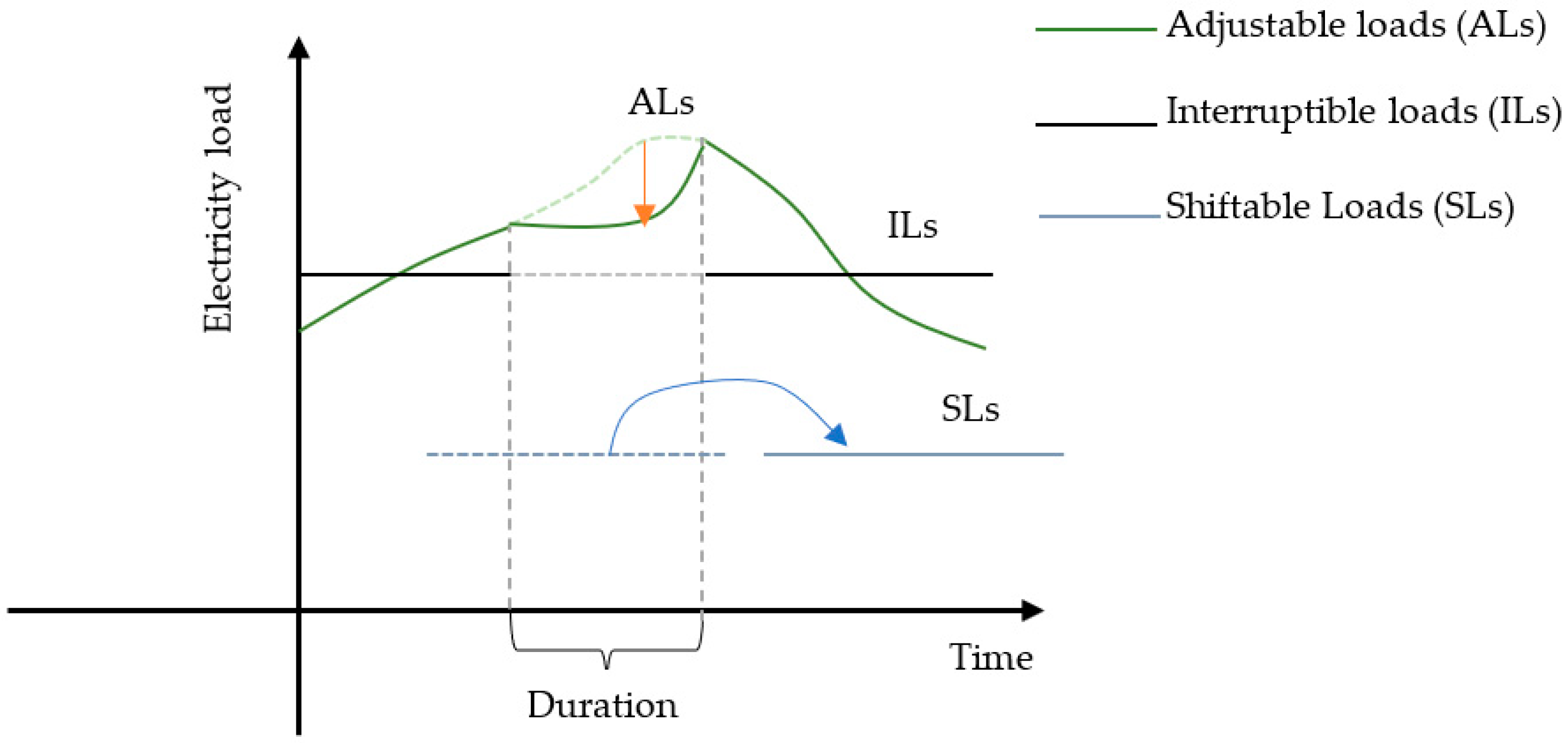
The classification of flexible loads based on a literature review can be seen in Figure 1. Interruptible Loads (ILs), which can be quickly curtailed under economic incentives, are common in industrial buildings. Shiftable loads (SLs) can be moved from peak to off-peak periods within a specified time window that we introduce in Section 2.2, offering flexibility without task compromise, and adjustable loads (ALs), found in both fixed equipment (e.g., lighting) and HVAC systems, whose power consumption can be regulated during peak demand periods.

1.2.1. Interruptible Loads (ILs)

ILs typically represent an ideal flexible resource, as they have relatively low reliability requirements from the power grid. Under certain economic compensation conditions, it can be conditionally curtailed during specific periods, enabling rapid DR [19]. ILs are prevalent in industrial buildings; for example, industrial production lines may be temporarily shut down during summer peak electricity demand periods to obtain DR subsidy [20]. The capacity and interruption duration of ILs are two evaluation factors for this flexible load type.

1.2.2. Shiftable Loads (SLs)

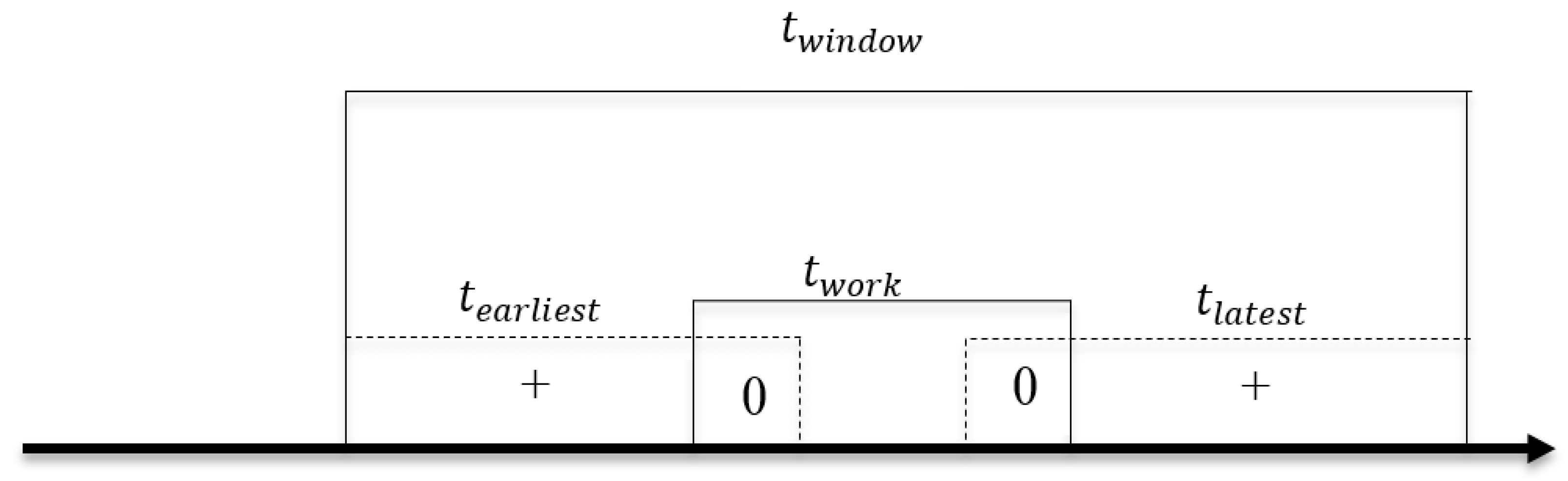
SLs refer to electrical equipment whose operation can be moved from peak load periods to off-peak periods and which typically do not operate continuously throughout the day. The precondition for equipment providing load shifting flexibility is that its time window (as shown in Figure 2) for operation is greater than its actual working duration. The concepts of time window and working window can be found in our previous study [3,21] and in Section 2.2. If an SL’s working window does not overlap with peak electricity demand periods, it may not provide effective load flexibility. Within the designated time window, SLs can be freely configured, offering load flexibility without compromising tasks. Examples include washing machines, dishwashers, energy storage devices, electric vehicles and so on.
SLs are widely used in residential buildings [22]. In DR programs, the SL device usually operates in two modes. Continuous operation, where the device, once started, cannot be interrupted until the task is completed, and interruptible operation, where the device can be paused if the scheduled task can be completed within the time window.

1.2.3. Adjustable Loads (ALs)

ALs refer to loads whose power consumption can be regulated during the DR period. Two types of AL commonly exist in buildings: fixed loads, such as lighting, and variable loads, influenced by external environmental conditions, such as HVAC loads. The load reduction ratio, which represents the proportion of load that can be regulated, is a key factor for ALs. Previous research indicates that lighting in office buildings can achieve a load reduction ratio of up to 0.8 during peak hours, with an average daily value of 0.2 [23]. For HVAC systems, load adjustment, such as resetting the zone temperature, can yield a load reduction ratio ranging from 0.1 to 0.5 [11]. When employing pre-cooling techniques, the load reduction ratio during peak periods can be even higher [24].
This paper introduces a comprehensive framework for optimizing building DR strategies by categorizing flexible loads and defining DR optimization objectives. Three DR objectives include maximizing load reduction, maximizing economic benefits, and ensuring stable load reduction with smooth recovery, addressing the control problems in real-world DR programs. The effectiveness of these strategies is demonstrated through case studies of both residential and office buildings, providing quantitative insights into achievable load reductions and cost savings under diverse scenarios, which serve as a valuable benchmark for future DR implementations. Finally, recommended DR control methods based on load flexibility characteristics are offered for grid-interactive buildings. Compared with previous studies utilizing simulation tools such as EnergyPlus and TRNSYS, the innovation of this work lies in proposing a formulation framework to quantify the flexibility capacity of various building loads, as well as developing more easily deployable control strategies for practical DR projects.
The remainder of this paper is organized as follows. Section 2 details DR control strategies, establishes electricity flexibility quantification formulations, and defines three DR optimization objectives. Section 3 presents two case studies, a residential building in Potsdam (winter DR) and an office building in Shanghai (summer DR). Section 4 summarizes the key findings and gives limitations and future research directions.

2. Methodology

This section introduces the methods used in this paper. First, four control strategies are introduced, including global zone temperature resetting, pre-cooling, smooth system recovery strategy, and others such as lighting dimming and water storage utilization. Second, three DR optimization objectives, including maximizing load reduction (Objective 1), maximizing economic benefits (Objective 2), and ensuring stable load reduction with smooth recovery (Objective 3), are proposed.

2.1. DR Control Strategies

2.1.1. Global Zone Temperature Resetting

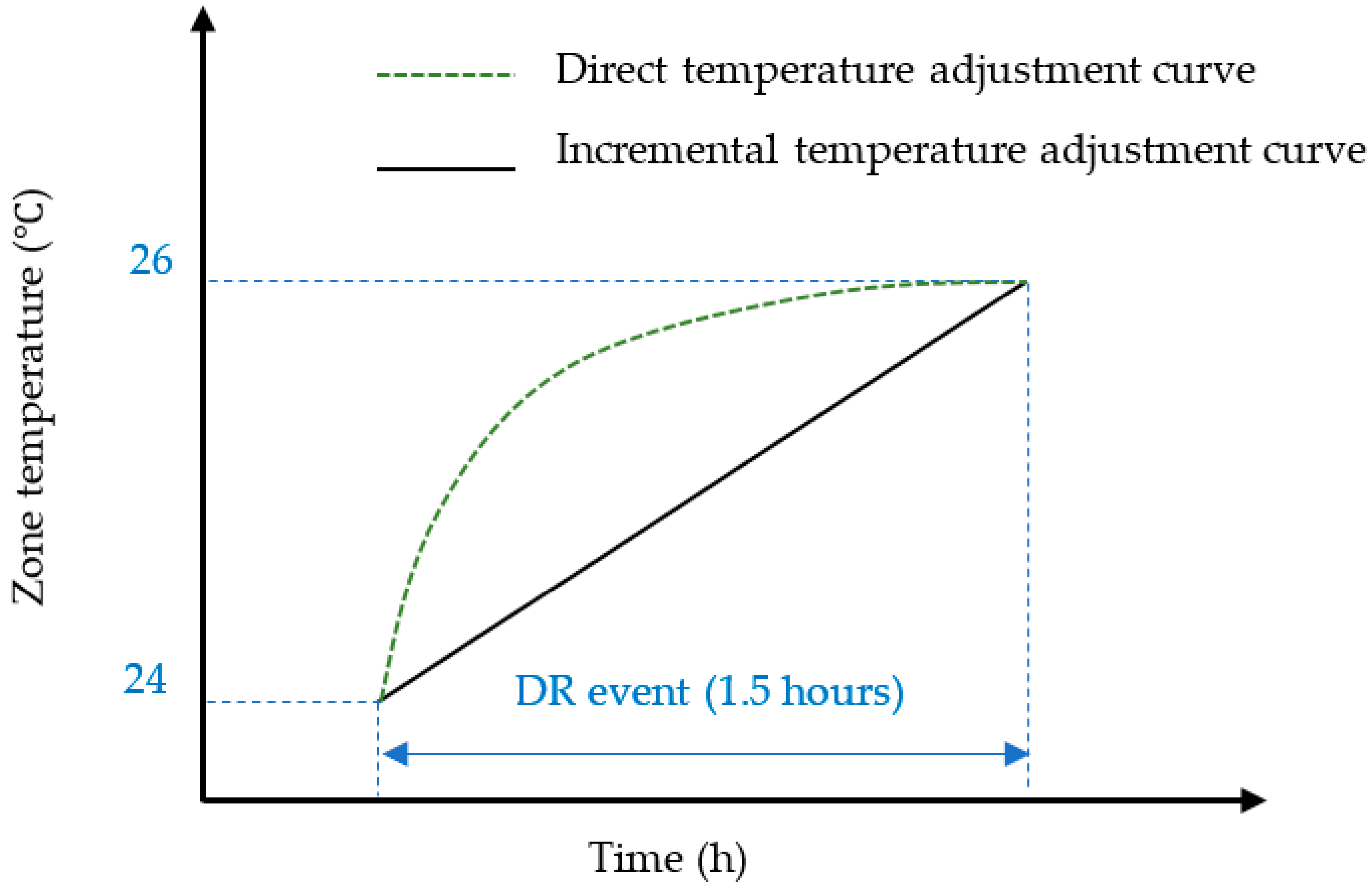
Zone temperature resetting relates to modifying the zone setpoint temperature. During DR events, for example, the maximum temperature adjustment typically does not exceed 3 °C to avoid occupant discomfort. However, with economic incentives for different occupants, a larger temperature adjustment range might be acceptable [3]. Based on the adjustment method, direct adjustment and incremental adjustment are introduced. Direct temperature adjustment means immediately setting the zone temperature to the target temperature. Incremental adjustment, conversely, utilizes a control system to gradually increase the temperature over a specified period, for example, a 2 °C increase within 1.5 h, as illustrated in Figure 3. Incremental adjustment allows for a more uniform temperature rise, mitigating the risk of thermal discomfort for occupants and facilitating smooth load reduction.

2.1.2. Pre-Cooling

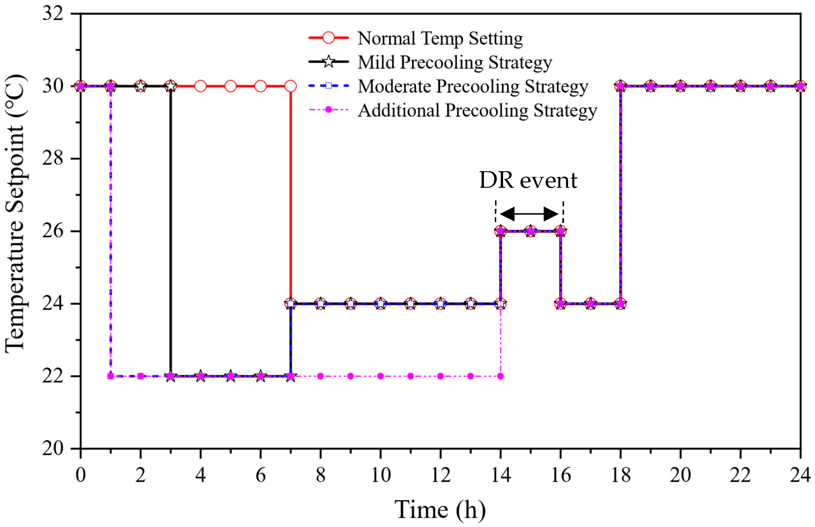
Pre-cooling is a strategy to cool the building envelope and internal thermal mass during off-peak electricity periods to reduce the building’s peak cooling load. Through pre-cooling, the peak cooling load can be shifted to off-peak periods, thereby leveraging the thermal inertia of the building’s thermal mass to decrease peak cooling demand. Figure 4 illustrates the hourly zone temperature setpoint under four different pre-cooling strategies, normal, mild, moderate, and additional pre-cooling, where the zone setpoint temperature during peak load periods is a consistent setting (e.g., 26 °C). The normal temperature setting serves as the baseline for comparison. Mild and moderate pre-cooling strategies consider setting the zone temperature to a lower value (e.g., 22 °C) before zone occupancy to moderately pre-cool the building. During zone occupancy, the setpoint temperature is set to a higher value (e.g., 24 °C or 26 °C) during peak periods. As shown in Figure 4, mild pre-cooling begins at 3:00 AM, while moderate pre-cooling starts earlier, at 1:00 AM. Additional pre-cooling also begins at 1:00 AM but aims to maintain the pre-cooled state until the peak load period.
Due to additional losses associated with cold storage and heat transfer, pre-cooling strategies typically result in an increase in total building energy consumption. However, they enable the shifting of a portion of the peak load to valley periods. For both building owners and society, electricity generated during peak periods is often the most expensive and polluting. Therefore, different pre-cooling strategies can lead to varying optimization approaches, either maximizing load reduction or maximizing economic benefits.

2.1.3. Smooth System Recovery Strategy

The smooth system recovery strategy is a method to prevent rebound peaks, primarily encompassing two approaches: gradual temperature recovery and extended DR control duration. For instance, after a DR event ends, room temperature recovery can be implemented incrementally, as shown in Figure 3. Extending the DR control duration typically means extending the DR control period beyond the end of the DR event, when the electricity load has already decreased, thereby avoiding the occurrence of a secondary peak demand to the power grid.

2.1.4. Other Strategies

To achieve bigger electricity load reduction, DR control for other equipment is also considered. This primarily includes reducing lighting intensity, utilizing energy storage systems, and extending the time windows of electrical equipment. Detailed control strategies are presented in Table 1.

2.2. Electricity Flexibility Quantification

For different load types, the quantification method differs. ILs are easy to quantify, as their flexibility equals the power load of the interruptible equipment. The other two types of SLs and ALs are described below in detail.

2.2.1. SLs Flexibility

SLs such as washing machines, dishwashers, dryers, and electric vehicles can be easily rearranged if the time window is longer than their operating time (working window). An illustration of the time window and working window is provided in Figure 2. No flexibility exists when the time window equals the working window, while a longer time window is more conducive to improving the flexibility of SLs, as it allows more space for load shifting and rescheduling. Equation (1) is used to calculate the electrical flexibility of SLs.
F s l = i = 1 n   P i t · γ i t
γ t = 0                 t t w o r k t e a r l i e s t + ( t w o r k t l a t e s t ) 1                 t t w i n d o w t w o r k 1                 t t w o r k t e a r l i e s t t l a t e s t
where twork is the work window and twindow is the time window; twork, can be freely moved inside the time window; tearliest and tlatest are the earliest and latest working windows, respectively; P i t is the appliances’ power; and γ i ( t ) is the flexibility state, which is defined in Equation (2).

2.2.2. ALs Flexibility

For ALs such as HVAC systems, when the thermal zone setting temperature changes, the HVAC system’s load is influenced. The HVAC systems’ electricity flexibility is coupled with the parts of thermal mass i = 1 n α i C i T r a n g e / ( t d C O P A C ) , which are explained in our previous work [3]; heat gain reduction from lights ( k 0 P l i g h t s ); room air heat inertia ( ρ a V r c a t d T r a n g e ); fresh air processing ( m ˙ c a T r a n g e ); and heat transferred from exterior walls ( U A T r a n g e ). The electricity flexibility of the HVAC systems is defined as Equation (3). Furthermore, the storage tank can be charged by chillers during the night or low-electricity-price time and can discharge stored heating/cooling load during peak electric time or high-electricity-price time. With the storage tank, the HVAC systems can provide a higher flexibility potential and longer flexibility response span. The electricity flexibility of the storage tank is defined as Equation (4).
F A L , H V A C = i = 1 n α i C i T r a n g e / ( t d C O P A C ) + [ k 0 P l i g h t s + ( ρ a V r c a t d + U A + m ˙ c a ) T r a n g e ] / C O P A C
F A L , t a n k = c w · ρ w · V t a n k · T t a n k ,     t 0 T t a n k ,   t d t d / C O P A C
where T r a n g e is the comfort temperature setting range; t d is the response span for the flexibility evaluation period or the demand-response period; C i is the total heat capacity of the building thermal mass; α i is the heat release ratio of thermal mass; C O P A C is the coefficient of performance of the air conditioning system; k 0 is the appliance power reduction ratio; ρ a is the density of air; c a is the heat capacity of air; V r is the thermal zone volume; U A is the overall heat transfer coefficient; m ˙ is the mass flow of fresh air; c w is the heat capacity of water; ρ w is the density of water; V t a n k is the volume of the tank; and T t a n k ,   t 0 and T t a n k ,   t d are the initial tank temperature and tank temperature after time span t d , respectively.

2.3. DR Optimization Objectives

Three optimization control objectives, including maximizing load reduction (Objective 1), maximizing economic benefits (Objective 2), and maintaining stable load reduction and recovery (Objective 3), are proposed. Objective 1 aims to achieve the largest total load reduction. Objective 2 seeks to maximize the economic gains for the building by considering DR subsidies and electricity bill savings. Objective 3 focuses on maintaining a smooth reduction while achieving the target reduction during the response period, particularly avoiding the occurrence of a secondary peak load after the DR event. These three optimization objectives are detailed below, and the common control variables and their bounds can be seen in Table 2.

2.3.1. Objective 1: Maximizing Load Reduction

In situations such as extreme weather events, natural or human-made disasters, and temporary equipment failures, the grid often requires users to reduce their electricity load as much as possible within a short period. The duration of such DR events is usually short, typically lasting from half an hour to several hours. The following formulation is presented with the Objective 1 of maximizing load reduction during DR.
m a x   Q t o t a l = Q I L + Q S L + Q A L
m a x   Q t o t a l = 0 t d F I L + F S L + F A L d t
where Q I L , Q S L , Q A L are the total load reductions (kJ) for ILs, SLs and ALs, respectively. Equation (6) defines the relationship between load reduction and electrical flexibility. F represents the electrical flexibility of different building flexible loads (W) under DR scenarios.
SLs are constrained by their time windows. The problem of maximizing SLs’ reduction can be transformed into minimizing the actual required load during the DR period, as shown in the following equation:
m a x     Q S L =   m i n i n θ = t d , s t d , e X i , θ P S L , i ( θ )
where i corresponds to the shiftable device; θ is the time step; X i , θ is the operating state of the shiftable device (0 for off, 1 for on); P S L , i ( θ ) is the power consumption of the shiftable device (W).
The problem is to minimize the overlap between the working window t w o r k in the DR period t d within the shiftable time window t w i n d o w , as shown in Figure 2. This overlap minimization problem can be further transformed into maximizing the distance from the center, i.e., maximizing the distance from the center of the t d and t w o r k , with the following equation:
m a x i = 1 n X i 2 t d , s + t d 2
The above equation can be converted into solving a non-linear minimization problem as follows:
m i n i = 1 n ( X i 2 t d , s + t d 2 ) 2
s . t .         X i + t w o r k 2   t w i n d o w , e
X i + t w o r k 2 t w i n d o w , s
where X i is the center position of the equipment’s working time and s , e are the start and end time markers, respectively. The above optimization problem can be conveniently solved using non-linear solvers. For instance, the fmincon function in Matlab, a gradient-based solver, can be employed.
For ILs, the primary consideration is the maximum interruptible duration. For ALs, both the power reduction duration and the ratio need to be considered. The reduction ratio should comprehensively account for the risk of sacrificing user comfort and the upper and lower limits of equipment adjustability. The optimization equation is as follows:
max Q I L , Q A L   =   m i n i n θ = t d , s t d , e ( 1 S i , θ k i , θ ) P S L , i ( θ )
s . t .         θ = t d , s t d , s + t d X i , θ Δ θ = M i
S i , θ = 0,1
where k i , θ is the power reduction ratio for each piece of equipment. For ILs, k i , θ = 1 ; X i , θ is the adjustable status of each piece of equipment (0 for not adjustable, 1 for adjustable); Δ θ is the time step, calculated based on the adjustable frequency of the equipment, which can be in minutes or hours; and M i is the maximum allowable total reduction duration for each piece of equipment.
Usually, equipment is not allowed for frequent power adjustments over short periods, such as frequent starts and stops. Therefore, when solving such problems, the time step should not be too short. The choice of time step can be estimated based on the equipment’s adjustable frequency, which can be on a minute or hour scale.

2.3.2. Objective 2: Maximizing Economic Benefits

The U.S. Department of Energy categorizes DR into two types: incentive-based DR and price-based DR [25]. Incentive-based DR refers to a response where users reduce electricity consumption to receive compensation. Price-based DR occurs when users decrease electricity demand in response to rising electricity prices and increase demand during periods of lower prices. For building energy managers, different DR types necessitate distinct DR control strategies to maximize energy efficiency and economic benefits.
The following analysis examines optimal control strategies when the building’s DR objective is to maximize economic benefits. Unlike the problem of Objective 1, the economic benefit maximization problem, due to the shifting of some loads to other periods, should consider the overall daily revenue. The equation for this problem is as follows:
m i n C o s t = m i n θ = 0 1440 ζ θ P I L , θ + P S L , θ + P A L , θ θ = t d , s t d , e ψ θ P I L , θ + P S L , θ + P A L , θ / 60
s . t .         θ = 0 1440 P S L , θ = P S L , t o t a l   θ = 0 1440 P I L , θ = P I L , t o t a l θ = t 1 t 2 P I L , θ   θ = 0 1440 P A L , θ = k ¯ P A L , t o t a l
where ζ θ is the electricity tariff; ψ θ is the DR subsidy; k ¯ is the average power reduction ratio; and t 2 t 1 is the interruption duration.

2.3.3. Objective 3: Smooth Load Reduction and Recovery

Objective 3 of smooth load reduction and recovery implies that the grid requires users participating in DR to maintain a stable reduction throughout the response period, while also avoiding the occurrence of a secondary peak after the DR event. This is crucial because if multiple users simultaneously open their loads, it can lead to new grid instabilities or even higher secondary peak loads, which is detrimental to the stable operation of the power grid. Therefore, certain restrictions are imposed on the load reduction during the DR event. This objective, while aiming to achieve the maximum reduction target, as described in Equation (5), is also constrained by the conditions in Equation (12).
( P t 1 P t 2 ) ( t 2 t 1 ) ξ P t 1
where P t is the electrical load (W) at time t and ζ is the maximum allowable reduction percentage. The calculation time step can be in minutes, and the specific reduction ratio needs to comply with the grid’s specific requirements.

3. Results and Discussion

This section presents two case studies of a residential building and an office building to investigate the proposed control strategies and objectives for different building types participating in DR. The analysis focuses on the contribution of the three flexible load types under different control objectives, providing guidance for the efficient operation of a practical DR program. It is worth noticing that the real electricity tariff of these two cases is not the dynamic price and we used the real-time tariff, while for the other building case using a dynamic tariff, the proposed method can be implemented with no difference.

3.1. Residential Building Case Study

This residential building is located in Potsdam, northern Germany, and comprises eight apartments, representing a typical residential building type in the temperate climatic zone of central Europe. This study selects one apartment with a floor area of 110 m2 for analyzing different optimization objectives. Typically, this building has no cooling demand throughout the year. The research methodology presented in this paper is also applicable to heating scenarios; thus, this study investigates the heating load demand and its electrical flexibility, providing a reference for winter DR projects. The building’s HVAC systems consists of a heat pump system with a thermal storage tank, utilizing an electric heater to provide heat demand. Table 3 provides detailed information on the equipment. The building’s flexible loads originate from shiftable and adjustable equipment, with no interruptible flexible loads.
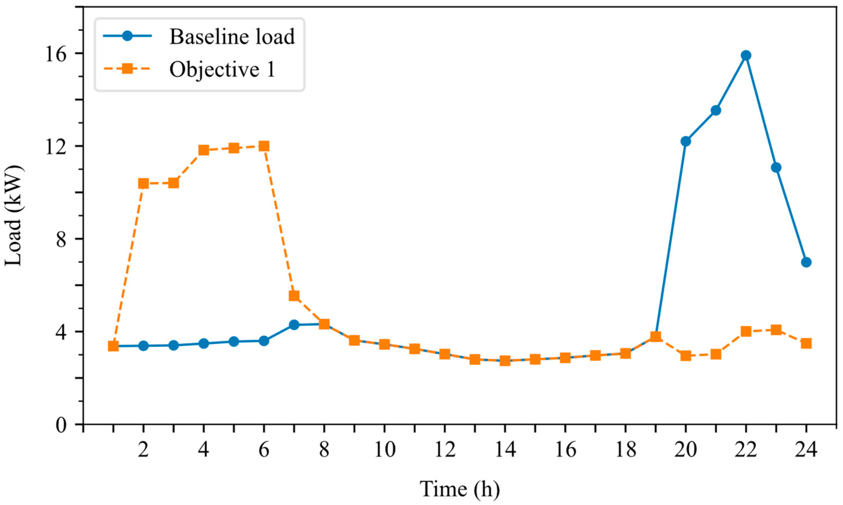
Unlike summer DR programs, the triggering period for residential building DR often occurs in the evening [26]. We analyze a common DR event from 19:00 to 21:00. To achieve different control objectives during this period, varying control strategies will be employed. For Objective 1, Figure 5 shows the load reduction curve during the DR period. Through SLs and Als control, the electricity load in the 19:00–21:00 period decreased from a baseline load of 12.87 kW to 2.60 kW, achieving a reduction of 79.83%. We considered that electric vehicles can only be charged in our study; if electric vehicles are considered capable of bidirectional interaction with the grid (i.e., both charging and discharging), the reduction would be even bigger.
Usually, some households do not own electric vehicles. Therefore, the analysis also considers scenarios without electric vehicles, as shown in Figure 6. Through SL and Al control, the electricity load in the 19:00–21:00 period decreased from a baseline load of 5.87 kW to 3.00 kW, representing a reduction of 49.02%, which is significantly lower than the scenario with an electric vehicle.
We can also observe that most of the load is shifted to the period between 4:00 AM and 6:00 AM, rather than late at night. This is because the load reduction maximization control algorithm maximizes the energy consumption of equipment within its time window to be as far as possible from the DR period. Load shifting to late-night hours, for example, between 0:00 AM and 4:00 AM, is desired by both the grid and users, and this can be achieved through economic benefit maximization methods.
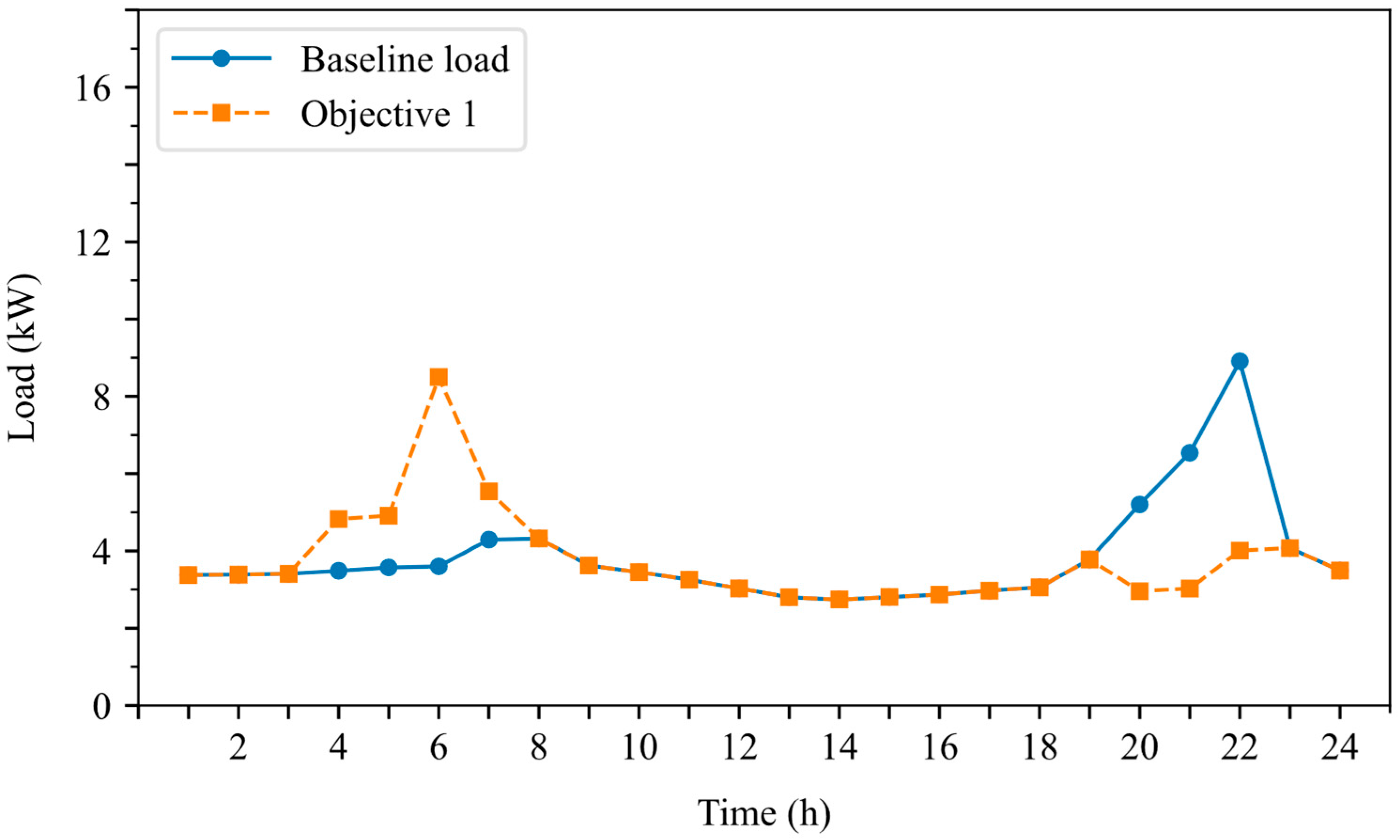
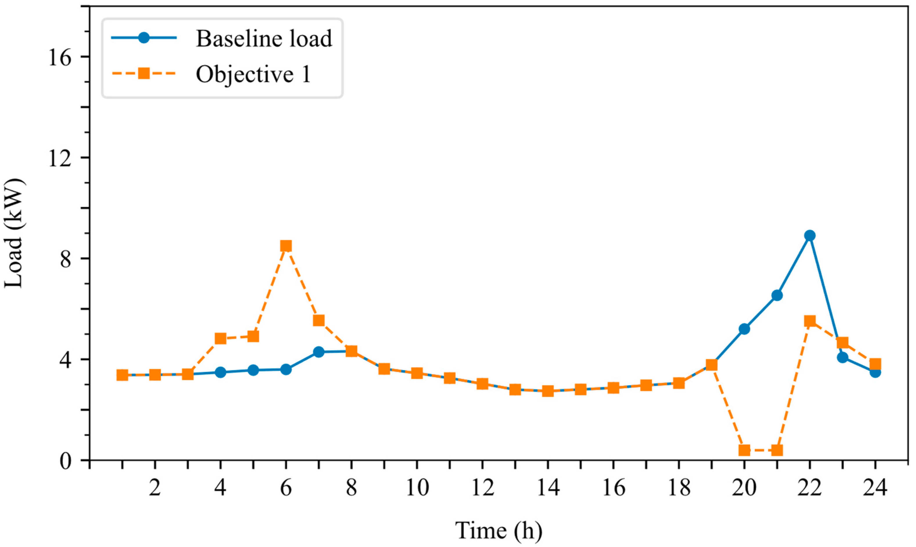
As the HVAC systems in this case study include a water storage tank, heating can be supplied to the system through the storage tank during the DR period, allowing the electric heater to be closed to reduce electricity demand. At the end of the DR (21:00), due to the lower tank temperature, the electric heater load rapidly increases, as shown in Figure 7. During the DR period, the building’s electricity load decreases from the baseline load of 5.87 kW to 0.40 kW. After the DR, the electricity load is 5.51 kW.
For Objective 2, electricity tariffs are a primary influencing factor. Currently, German residential electricity prices are fixed. Thus, this study simulates and analyzes using an electricity tariff and DR subsidy policies based on Shanghai. The peak and off-peak tariffs are 0.617 and 0.307 CNY/kWh, respectively. The peak period is from 6:00 to 22:00, and the off-peak period is from 22:00 to 6:00 the next day. The DR subsidy of 0.8 CNY/kWh is used.
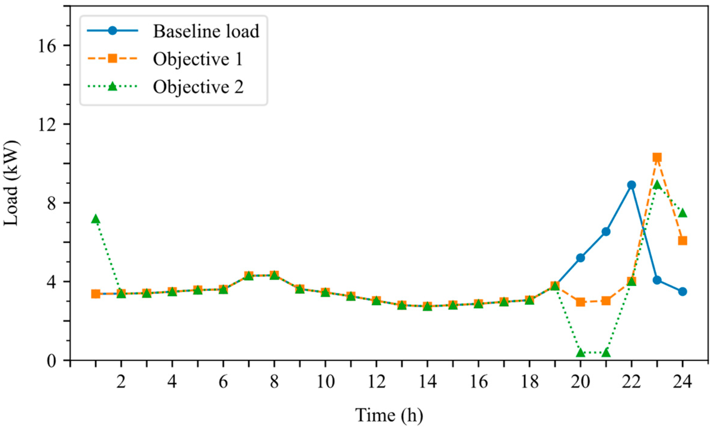
Without considering scenarios with electric vehicles (the same DR controls in Figure 7), this paper presents the optimized electricity load curve under Objective 2 control, and the results are shown in Figure 8. Compared to Objective 1, Objective 2 shifts most of the load to between 22:00 and 24:00, rather than the early morning hours. This is because a uniform off-peak electricity price is in effect from 22:00 to 6:00 the next day, and the control strategy prioritizes completing assigned tasks for each piece of equipment as early as possible within this off-peak window. With Objective 2 optimization control, the total electricity bills are 33.3 CNY and 39.5 CNY with and without the storage tank, achieving cost savings of 17.6% and 30.5%, respectively, compared to the total daily cost of CNY 47.9 without a DR event.
Since shiftable flexibility exhibits an on–off characteristic, it is not suitable for smooth reduction control. Therefore, the analysis of Objective 3 was conducted in the office building case only.

3.2. Office Building Case Study

The office building case is an office building in Shanghai. The total building area is 51,072 m2, with an air-conditioned area of 40,320 m2. This office building is equipped with a centralized air conditioning system with two chillers. The internal heat gains from occupancy, lighting, and equipment are 16 W/m2, 11 W/m2, and 13 W/m2, respectively. The heat transfer coefficients (U-values) of the external wall is 0.95 W/(m2·K). During DR events, load reduction in this office building is mostly from ALs, such as HVAC systems and lighting, with no ILs and SLs. Table 4 provides the information on the ALs in this building.
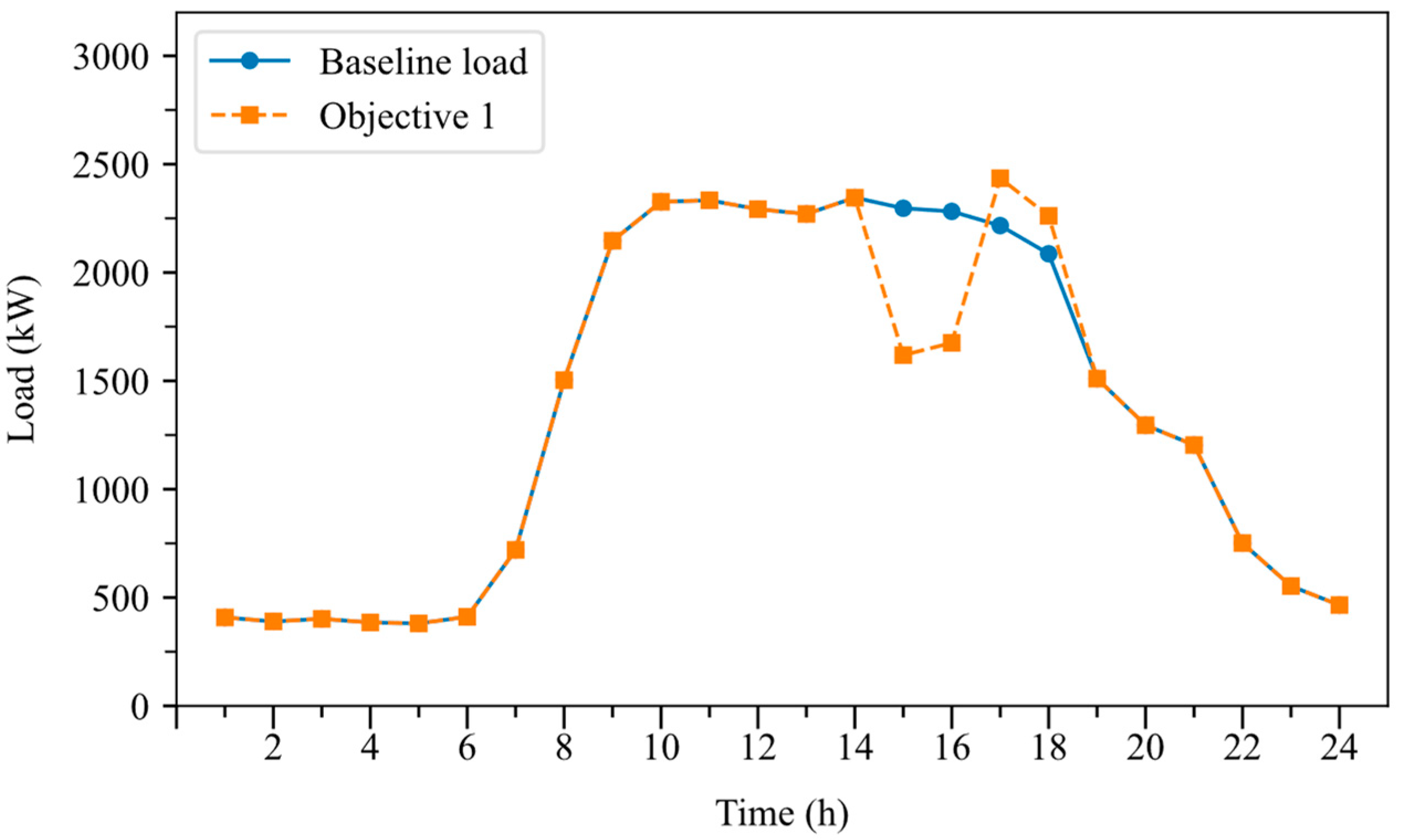
This paper analyzes a summer DR event from 14:00 to 16:00. The adopted DR control strategies include adjusting the HVAC systems, dimming the lighting, and utilizing water storage. The zone temperature is adjusted from 24 °C at the start of the DR (14:00) to 26 °C and then reset to 24 °C after the DR ends (16:00). During this period, lighting intensity is reduced by 40%. Figure 9 shows the load reduction curve for this building. As shown in the figure, significant load reduction occurs during the DR event, with the average electricity load decreasing from 2289 kW to 1647 kW, a reduction of 28.1%. After the zone temperature is reset to 24 °C, a secondary peak load of 2435 kW occurs.
Comparing the maximum load reduction for residential buildings, the office building shows a smaller peak load reduction. This is because SLs in residential buildings can shift most of the load to off-peak periods. However, for office buildings, incorporating water storage and considering higher acceptable zone temperature setting (e.g., 27 °C) could lead to bigger load reductions.
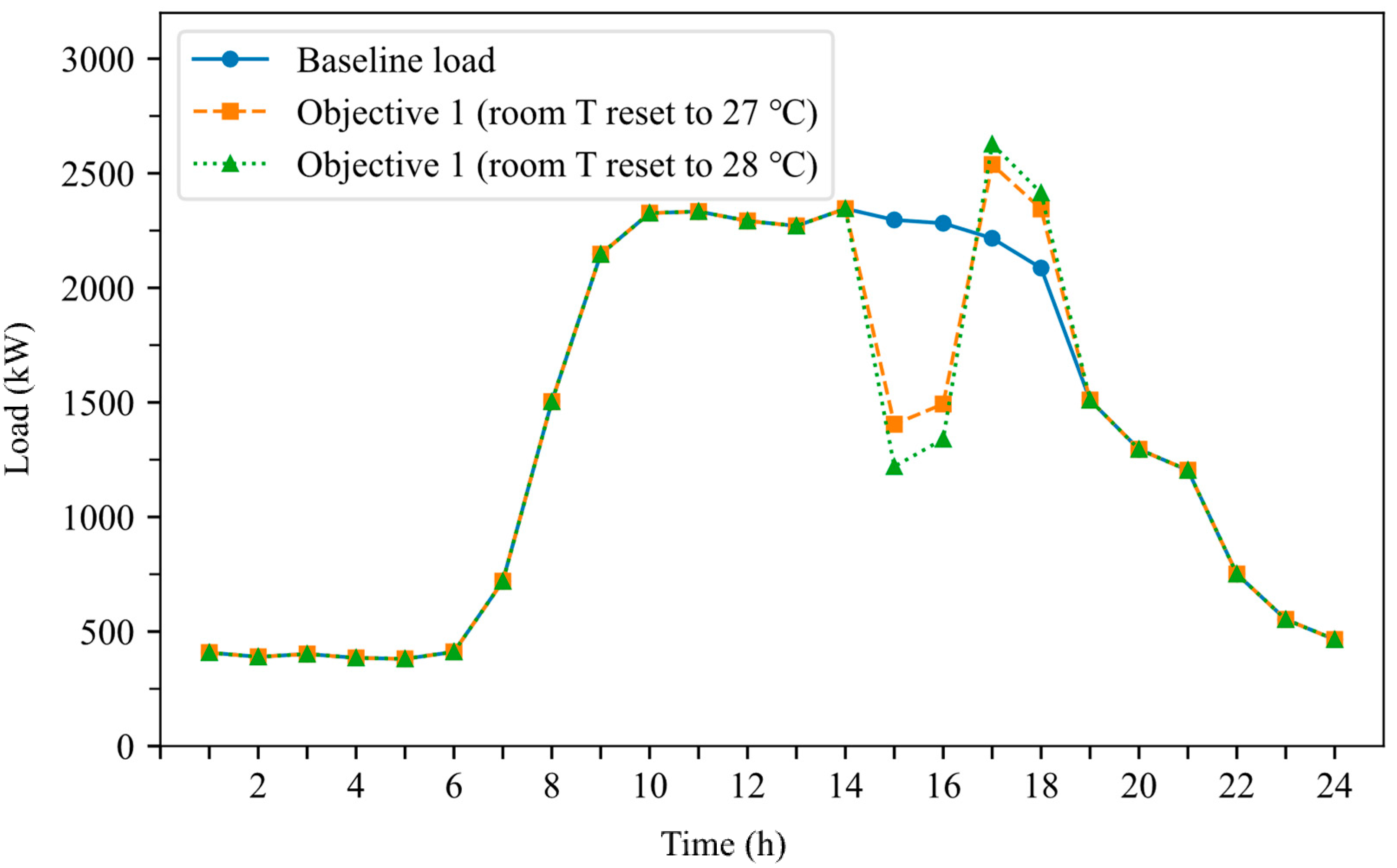
This case analyzes two scenarios with higher acceptable zone temperatures: one where the acceptable upper limit is set to 27 °C, and another where it is 28 °C. After the DR ends, the zone temperature setpoint is reset to 24 °C. Figure 10 shows the load reduction for these two scenarios. The average electricity load decreases from 2289 kW to 1450 kW and 1280 kW, respectively, corresponding to total electricity reduction rates of 36.7% and 44.1%. When the zone temperature is reset to 24 °C, secondary peak loads of 2538 kW and 2628 kW occur.
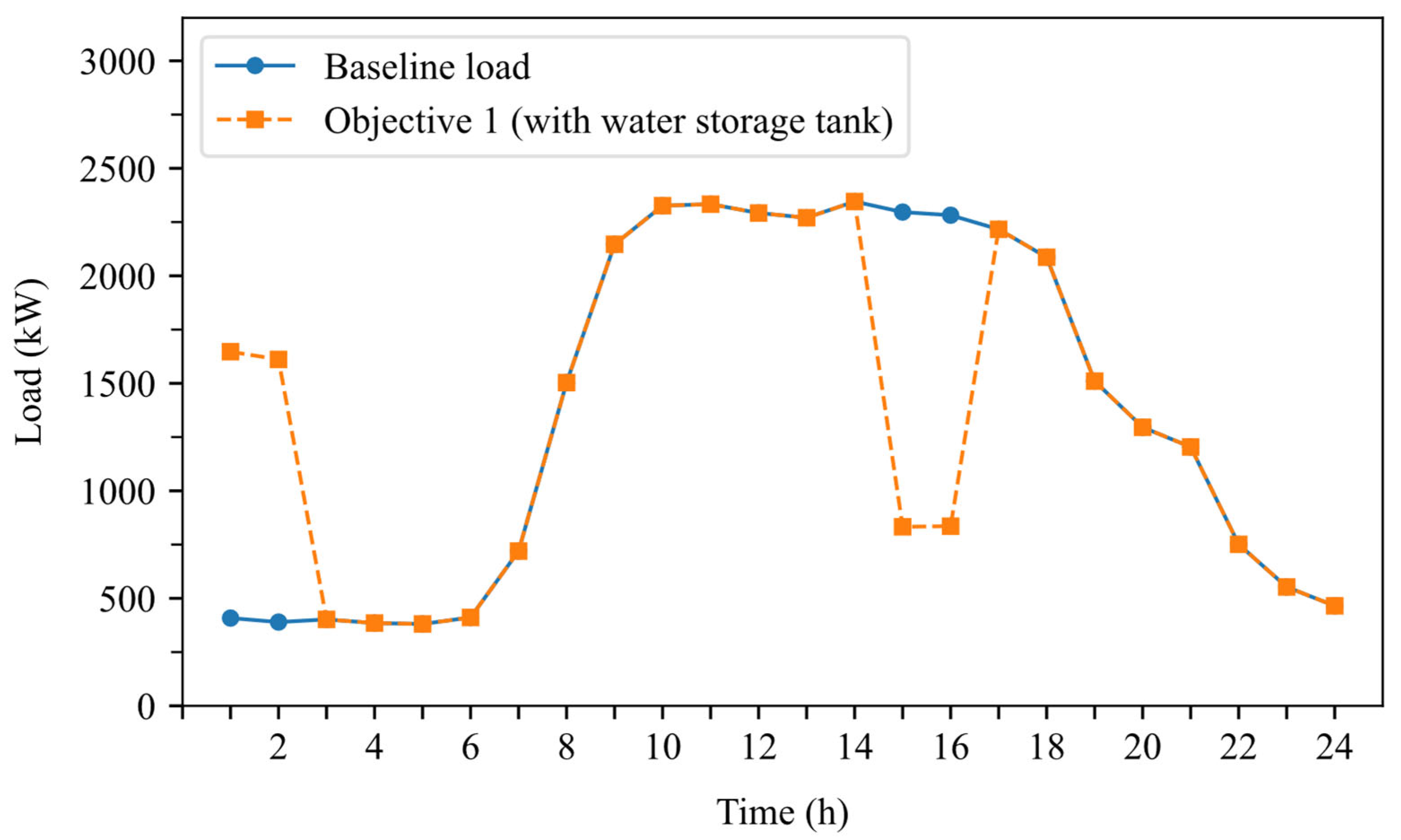
When the HVAC systems are integrated with chilled water storage, its reduction capability can be further enhanced. In this case study, the volume of the HVAC system’s water tank is 223.2 m3. When the water tank is used for cooling, the chillers can be shut down. In this scenario, the maximum HVAC system reduction equals the electricity load of the chiller. Figure 11 shows the load curve reduced by utilizing the energy storage tank. The average electricity load decreases from 2289 kW to 834 kW, representing a reduction of 63.6%. As shown in this figure, the peak load is shifted to the off-peak time, with the water storage tank utilizing off-peak electricity for cold storage.
To investigate DR control for maximizing benefits across different control strategies. Shanghai’s commercial summer electricity tariff for peak, flat, and valley periods are 1.257, 0.787, and 0.299 CNY/kWh, respectively. The peak, flat, and valley periods are divided as follows: peak periods are 8:00–11:00, 13:00–15:00, and 18:00–21:00; flat periods are 6:00–8:00, 11:00–13:00, 15:00–18:00, and 21:00–22:00; and valley period is 22:00–6:00 the next day. A value of 2 CNY/kWh of DR subsidy is considered.
Without DR control, the building’s daily electricity cost is approximately CNY 32,632. The electricity cost savings under different scenarios are shown in Table 5. Scenario 1 implements only adjusting the HVAC load by increasing the zone setpoint temperature by 2 °C, resulting in a total electricity cost saving of approximately 7.39%. If the temperature is increased by 4 °C (Scenario 2), the electricity cost saving increases to 13.88%. Considering a 40% reduction in lighting intensity together (Scenario 3 and Scenario 4), the electricity cost savings are 11.87% and 18.36%, respectively. Utilizing the chilled water storage tank for cooling (Scenario 5) achieves the maximum benefit, reaching 26.79%.
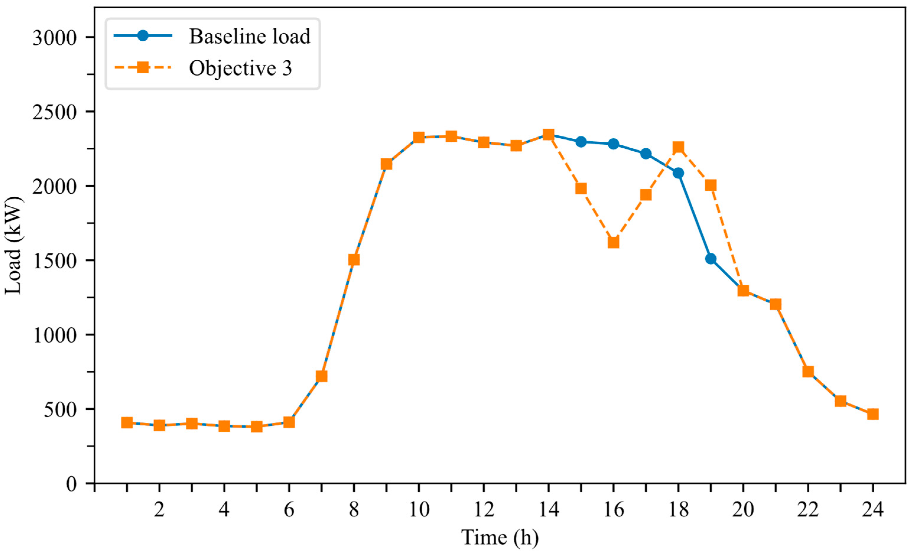
Regarding Objective 3, smooth load reduction and recovery, the DR program requires a gradual adjustment of room temperature, including temperature recovery after the DR ends. In this case, the indoor temperature setpoint gradually increases from 24 °C at the start of the DR to 26 °C over two hours. At the end of the DR, the temperature setpoint then recovers to 24 °C over another two hours. The smooth reduction curve is shown in Figure 12. The reduction ratio during the DR period is 21.4%, which is lower than the 28.1% reduction ratio for Objective 1. Compared to the control strategy for Objective 1, Objective 3 exhibits a smoother load reduction, with load reduction rates of −11.3 kW/min and −5.2 kW/min, respectively. The load increase rates after temperature recovery are 12.5 kW/min and 5.4 kW/min, respectively.

3.3. DR Control Recommendation

Based on the overall analysis, Table 6 presents recommended control methods for different DR optimization objectives, offering guidance for practical DR projects.

4. Conclusions

This study systematically categorized building electricity flexibility into interruptible loads (ILs), shiftable Loads (SLs), and adjustable loads (ALs) and subsequently developed and demonstrated optimal DR strategies based on their flexibility characteristics. The analysis elucidated the distinct response capabilities of each flexible load type. Namely, ILs offer rapid, real-time curtailment; SLs provide substantial peak shifting potential contingent on operational time windows; and ALs allow for modulated power consumption based on defined adjustment ratios and environmental conditions. Collectively, these flexible resources are pivotal for enhancing the grid-interactive capabilities. Furthermore, this study evaluated three critical DR optimization objectives: maximizing load reduction, an imperative for grid stability during peak events; maximizing economic benefits, a key motivation for building occupants and operators; and ensuring stable load reduction with smooth recovery, a crucial requirement to prevent secondary peaks and maintain grid reliability.
Through case studies of a residential building and an office building, we quantitatively illustrated the effectiveness of these DR strategies and optimization objectives. For the residential building, dominated by shiftable flexible loads including household appliances and electric vehicles, our optimization models achieved over 50% electricity load shifting during a 19:00–21:00 DR event, providing electricity bill savings exceeding 17.6%. In the office building case study, a 14:00–16:00 DR event leveraging integrated zone temperature resetting, lighting dimming, and water storage, demonstrated total electricity load reductions ranging from 28.1% to 63.6%, and associated electricity bill savings between 7.39% and 26.79%. These empirical results provide valuable benchmarks for assessing DR performance across diverse buildings and control strategies. Ultimately, this study not only establishes an overall formulation for the characterization and classification of building energy flexibility but also provides evidence-based practical guidelines for the deployment of effective DR control strategies. Consequently, simplified flexibility quantification methods and easy deployment control algorithms facilitate the realization of bidirectional coordination between the power grid and grid-integrated building energy systems.
This study has several limitations that warrant consideration for future research. First, the analysis relies on deterministic assumptions for weather conditions and occupancy patterns, overlooking the inherent variability of these factors in real-world scenarios, which may affect the robustness of the proposed DR strategies. Second, the current flexibility quantification framework does not account for uncertainties in equipment performance degradation, which may impact practical deployment. Future work should address these gaps by (1) incorporating stochastic weather and occupancy models to enhance strategy adaptability; (2) integrating personalized comfort models and user behavior dynamics to balance flexibility and occupant satisfaction; and (3) exploring the potential of AI-driven real-time optimization to further unlock building energy flexibility.

Author Contributions

Conceptualization, Y.C.; Methodology, Y.C. and Z.C.; Validation, H.Y.; Writing—original draft, H.Y.; Writing—review & editing, Y.C. and Z.C.; Visualization, H.Y.; Supervision, Y.C.; Funding acquisition, Y.C. All authors have read and agreed to the published version of the manuscript.

Funding

The authors greatly acknowledge the support from the National Natural Science Foundation of China (No. 52208116).

Data Availability Statement

The original contributions presented in the study are included in the article, further inquiries can be directed to the corresponding author/s.

Conflicts of Interest

The authors declare no conflict of interest.

References

  1. OECD. IEA Roadmap for Energy-Efficient Buildings and Construction in ASEAN: Timelines and Actions Towards Net Zero-Carbon Buildings and Construction; OECD: Paris, France, 2022; ISBN 978-92-64-44421-8. [Google Scholar]
  2. Ahmed, B.; Ahmed, A.; Zhang, H.-N.; Li, X.-B.; Qu, K.-Y.; Li, F.-C. Characterization, Quantification and Application of Energy Flexibility in Office Building: A Comprehensive Review. Energy Build. 2025, 347, 116306. [Google Scholar] [CrossRef]
  3. Chen, Y.; Chen, Z.; Xu, P.; Li, W.; Sha, H.; Yang, Z.; Li, G.; Hu, C. Quantification of Electricity Flexibility in Demand Response: Office Building Case Study. Energy 2019, 188, 116054. [Google Scholar] [CrossRef]
  4. Han, B.; Li, H.; Wang, S. A Probabilistic Model for Real-Time Quantification of Building Energy Flexibility. Adv. Appl. Energy 2024, 15, 100186. [Google Scholar] [CrossRef]
  5. Wang, H.; Wang, S.; Tang, R. Development of Grid-Responsive Buildings: Opportunities, Challenges, Capabilities and Applications of HVAC Systems in Non-Residential Buildings in Providing Ancillary Services by Fast Demand Responses to Smart Grids. Appl. Energy 2019, 250, 697–712. [Google Scholar] [CrossRef]
  6. Chen, Z.; Xiao, F.; Chen, Y. Multi-Objective Online Optimization of Building Energy Systems for Improved Control Smoothness and Efficiency. Autom. Constr. 2026, 181, 106604. [Google Scholar] [CrossRef]
  7. OpenADR: Connecting Smart Energy to the Grid. Available online: https://www.openadr.org/ (accessed on 8 November 2025).
  8. Newsom, G. 2025 Nonresidential Compliance Manual; California Energy Commission: Sacramento, CA, USA, 2025.
  9. Zhou, B.; Li, W.; Chan, K.W.; Cao, Y.; Kuang, Y.; Liu, X.; Wang, X. Smart Home Energy Management Systems: Concept, Configurations, and Scheduling Strategies. Renew. Sustain. Energy Rev. 2016, 61, 30–40. [Google Scholar] [CrossRef]
  10. Han, Y.; Gao, W.; Wang, Z.; Zhao, Q. Optimizing Grid-Interactive Buildings Demand Response: Sequence-Based Decision-Making Multi-Agent Policy Decomposition Deep Reinforcement Learning. Energy Build. 2025, 347, 116198. [Google Scholar] [CrossRef]
  11. Aduda, K.O.; Labeodan, T.; Zeiler, W.; Boxem, G.; Zhao, Y. Demand Side Flexibility: Potentials and Building Performance Implications. Sustain. Cities Soc. 2016, 22, 146–163. [Google Scholar] [CrossRef]
  12. Chen, Z.; Zhang, J.; Xiao, F.; Xu, K.; Chen, Y. Development of a Probabilistic Cooling Load Prediction-Based Robust Chiller Sequencing Strategy and Its Real-World Implementation. Appl. Energy 2025, 382, 125213. [Google Scholar] [CrossRef]
  13. Wang, T.; He, J.; Li, Y. Cooling Demand Response-Based Collaborative Optimization on the Supply and Demand Side of District Cooling System under Extreme Heat. Sustain. Cities Soc. 2025, 130, 106550. [Google Scholar] [CrossRef]
  14. Chen, Z.; Xiao, F.; Xiao, Z.; Chen, Y. Bridging the Gap between Data-Driven Baselines and Energy Saving Uncertainty for Building Retrofit. Energy 2025, 340, 139292. [Google Scholar] [CrossRef]
  15. Wu, H.; Qiu, D.; Zhang, L.; Sun, M. Adaptive Multi-Agent Reinforcement Learning for Flexible Resource Management in a Virtual Power Plant with Dynamic Participating Multi-Energy Buildings. Appl. Energy 2024, 374, 123998. [Google Scholar] [CrossRef]
  16. Cao, L.; Hu, P.; Li, X.; Sun, H.; Zhang, J.; Zhang, C. Digital Technologies for Net-Zero Energy Transition: A Preliminary Study. Carbon Neutrality 2023, 2, 7. [Google Scholar] [CrossRef]
  17. Xu, K.; Chen, Z.; Xiao, F.; Zhang, J.; Zhang, H.; Ma, T. Semantic Model-Based Large-Scale Deployment of AI-Driven Building Management Applications. Autom. Constr. 2024, 165, 105579. [Google Scholar] [CrossRef]
  18. Lee, J.; Li, J.; Yoon, S. From Design to Operation: Multi-Agent AI for Virtual in-Situ Modeling of Digital Twins in BIM. Autom. Constr. 2025, 179, 106477. [Google Scholar] [CrossRef]
  19. Chen, Y.; Zhang, L.; Xu, P.; Di Gangi, A. Electricity Demand Response Schemes in China: Pilot Study and Future Outlook. Energy 2021, 224, 120042. [Google Scholar] [CrossRef]
  20. Wang, J.; Bloyd, C.N.; Hu, Z.; Tan, Z. Demand Response in China. Energy 2010, 35, 1592–1597. [Google Scholar] [CrossRef]
  21. Yongbao, C. Study on Electricity Flexibility and Flexibility Evaluation of Demand Response Buildings; Tongji University: Shanghai, China, 2020. [Google Scholar]
  22. Berg, B.; Kunwar, N.; Guillante, P.; Vanage, S.; Mahmud, R.; Cetin, K.; Jahanbani Ardakani, A.; McCalley, J.; Wang, Y. Occupant-Driven End Use Load Models for Demand Response and Flexibility Service Participation of Residential Grid-Interactive Buildings. J. Build. Eng. 2024, 96, 110406. [Google Scholar] [CrossRef]
  23. Sehar, F.; Pipattanasomporn, M.; Rahman, S. An Energy Management Model to Study Energy and Peak Power Savings from PV and Storage in Demand Responsive Buildings. Appl. Energy 2016, 173, 406–417. [Google Scholar] [CrossRef]
  24. Turner, W.J.N.; Walker, I.S.; Roux, J. Peak Load Reductions: Electric Load Shifting with Mechanical Pre-Cooling of Residential Buildings with Low Thermal Mass. Energy 2015, 82, 1057–1067. [Google Scholar] [CrossRef]
  25. U.S. Department of Energy. Benefits of Demand Response in Electricity Markets and Recommendations for Achieving Them; U.S. Department of Energy: Washington, DC, USA, 2006.
  26. Nan, S.; Zhou, M.; Li, G. Optimal Residential Community Demand Response Scheduling in Smart Grid. Appl. Energy 2018, 210, 1280–1289. [Google Scholar] [CrossRef]
Figure 1. Illustration of different flexible loads.
Buildings 15 04368 g001
Figure 2. Illustration of the time window and the working window. (+ means positive flexibility, 0 means no flexibility).
Buildings 15 04368 g002
Figure 3. Illustration of direct and incremental temperature adjustment.
Buildings 15 04368 g003
Figure 4. Temperature setting of different pre-cooling strategies.
Buildings 15 04368 g004
Figure 5. Load curve under objective 1 (DR strategies: controlled equipment includes washing machine, dishwasher, dryer, electric vehicle, lighting, and HVAC systems).
Buildings 15 04368 g005
Figure 6. Load curve under objective 1 (DR strategies: controlled equipment includes washing machine, dishwasher, dryer, lighting, and HVAC systems).
Buildings 15 04368 g006
Figure 7. Load curve under objective 1 (DR strategies: controlled equipment includes washing machine, dishwasher, dryer, lighting, HVAC systems, and water storage).
Buildings 15 04368 g007
Figure 8. Load curve under objective 2 (DR strategies: controlled equipment includes washing machine, dishwasher, dryer, lighting, HVAC systems, and water storage).
Buildings 15 04368 g008
Figure 9. Load curve under objective 1 (DR strategies: indoor temperature reset from 24 °C to 26 °C; lighting intensity reduced by 40%).
Buildings 15 04368 g009
Figure 10. Load curve under objective 1 (DR strategies: indoor temperature adjusted from 24 °C to 27 °C and 28 °C, respectively; lighting intensity reduced by 40%).
Buildings 15 04368 g010
Figure 11. Load curve under objective 1 (DR strategies: chiller shut down, direct cooling from water storage tank; lighting intensity reduced by 40%, and zone temperature is 24 °C).
Buildings 15 04368 g011
Figure 12. Load curve under objective 3 (DR strategies: incremental indoor temperature adjustment; lighting intensity reduced by 40%).
Buildings 15 04368 g012
Table 1. Other DR control strategies.
DR Control StrategySpecific Implementation Methods
Reduce lighting intensity
(lighting dimming)
  • Reduce lighting intensity (e.g., 40%) during DR event;
  • Turn off lighting when natural light intensity reaches 500 lx.
Utilize energy storage
  • Install water storage tank for cooling and heating;
  • Install battery storage systems.
Extend time window
  • Extend dishwasher time window (e.g., 20:00–7:00 am next day);
  • Extend washing machine time window (e.g., 19:00–7:00 am next day);
  • Extend electric vehicle charging time window (e.g., 18:00–8:00 am next day);
  • Appropriately extend time windows for other electrical equipment.
Table 2. Detailed information on the control variables.
Variable NameDescriptionValue Bounds
Zone temperature settingThe comfortable and acceptable temperature setting in the zoneCooling case: 22–26 °C
Heating case:18–23 °C
Temperature   setting   range   T r a n g e The change in temperature settings 0–2 °C
Time window twindowThe time range when the appliances can be workingBased on appliance types and users’ preference
Working window tworkThe total working hours of the appliancesBased on appliance types and users’ preference
Power   reduction   ratio   k 0 The ratio of total power that can be reduced 0.2–0.6
Table 3. Parameters for flexible equipment types in the residential building case.
Equipment TypeEquipment
Name
Rated Power (kw)Daily Working Window (h)Time Window (h) (End Time)
Shiftable flexible loads
(SLs)
Washing machine1.342.0 (19:00–21:00)7.5 (4:00 am)
Dishwasher1.252.0 (20:00–22:00)8.5 (6:00 am)
Dryer3.651.0 (21:00–22:00)8.0 (5:00 am)
Electric vehicle (nissan leaf 30 kwh, 7 kw charging power)7.004.5 (19:00–23:30)8.5 (5:00 am)
Adjustable flexible loads
(ALs)
Equipment nameRated power (kw)Load reduction ratioAdjustable duration
Lighting0.660.4 (6:00–8:00, 18:00–23:00)Throughout DR event
HVAC systems (heat pump& storage tank)4.500.2 (all day, reduce heating load when unoccupied)Throughout DR event
Table 4. Parameters for ALs in the office building case.
Equipment NameRated Power
(kW)
Load Reduction RatioAdjustable Duration
Adjustable flexible loads (ALs)Lighting5620.4 (8:00–20:00)Throughout DR event
Chiller561 × 2Based on flexibility capabilities
(8:00–20:00)
Throughout DR event
Other HVAC System493.5Based on cooling and fresh air demand (8:00–20:00)Throughout DR event
Table 5. Economic benefits under different DR control scenarios.
Demand-Response Control ScenarioOptimized Electricity Cost (CNY)Electricity Cost Savings (CNY)Electricity Cost Savings Ratio
Scenario 1: room temperature resetting from 24 °C to 26 °C30,22224107.39%
Scenario 2: room temperature resetting from 24 °C to 28 °C28,103452913.88%
Scenario 3: lighting intensity reduced by 40% and room temperature resetting from 24 °C to 26 °C28,758387411.87%
Scenario 4: lighting intensity reduced by 40% and room temperature resetting from 24 °C to 28 °C26,640599318.36%
Scenario 5: lighting intensity reduced by 40% and chilled water storage cooling23,890874226.79%
Table 6. Recommended DR control strategies for different optimization objectives.
DR Optimization ObjectivesRecommended DR Control Strategies by Priority
Objective 1: maximize load reduction
(1)
Direct reset zone temperature: increase the zone setpoint temperature by 2 °C; if permitted by users, 3–4 °C could be acceptable.
(2)
Pre-cooling: set lower room temperatures (e.g., 22 °C) at night or before peak electricity demand to cool the internal thermal mass of the building.
(3)
Install energy storage devices: include thermal water storage tanks in cooling and heating systems and battery storage in energy systems.
(4)
Reduce lighting intensity: reduce room lighting load by 20–60%under sufficient natural light conditions, while ensuring that room illumination remains within a comfortable range (above 500 lx).
(5)
Extend equipment time window: for household appliances like washing machines and dishwashers, and charging devices, schedule their operation to avoid the DR period.
Objective 2: maximize economic benefits
(1)
Adjust zone temperature and pre-cooling.
(2)
Install energy storage devices.
(3)
Reduce lighting intensity.
(4)
Extend equipment time window.
Objective 3: smooth load reduction and recovery
(1)
Incremental temperature adjustment: gradually increase the zone setpoint temperature, e.g., a 2 °C increase over two hours.
Disclaimer/Publisher’s Note: The statements, opinions and data contained in all publications are solely those of the individual author(s) and contributor(s) and not of MDPI and/or the editor(s). MDPI and/or the editor(s) disclaim responsibility for any injury to people or property resulting from any ideas, methods, instructions or products referred to in the content.