Linking Visual Perception of Urban Greenery to Resident Preference in High-Density Residential Areas Through Mobile Point-Cloud-Based Assessment

Abstract

Urban greenery is essential for environmental quality, visual comfort, and residents’ well-being, and it becomes especially critical in high-density residential compounds where outdoor space is limited. This study proposes a pedestrian-scale visibility framework that integrates solid 3D models (DEM, extruded buildings, water) with voxelized LiDAR point clouds to reconstruct fine-resolution outdoor scenes and to quantify visual perception indicators, including green view factor (GVF), sky view factor (SVF), and average green distance (AGD). A residential community in Nanjing is used as the case study. Line-of-sight sampling was performed on 223 viewpoints distributed across three empirically identified activity zones, and a resident questionnaire was conducted in parallel (279 valid responses). The results show that the visually open zone, characterized by relatively high SVF, moderate GVF, and larger vegetation setback (higher AGD), is also the zone most preferred by residents, whereas the zone with the highest GVF but strong enclosure is least preferred. This consistency between modeled indicators and survey responses confirms that excessive, close-range planting may reduce usability, while a balanced combination of greenery and openness better supports everyday outdoor activities. The proposed Point-Cloud-Based approach, therefore, provides a data-driven basis for planning, evaluating, and managing outdoor environments in dense urban residential areas, and ultimately reaching the purpose of more livable urban communities in the era of intelligent and sustainable cities.

1. Introduction

Urban greenery plays a vital role in shaping environmental quality, visual comfort, and residents’ well-being, serving as a key component of sustainable and health-oriented urban design. In China, the process of rapid urbanization has reshaped the spatial structure of cities and increased the prevalence of high-density built environments. According to publicly available data, China’s urbanization ratio (i.e., the share of population living in urban areas) reached 67% by the end of 2024 [1]. In rapidly urbanising cities, high-density built environments may harm residents’ mental health and emotional well-being [2,3,4], but empirical and epidemiological studies show that sufficient exposure to urban greenery can mitigate these psychological impacts [5,6]. Urban greenery is one of the effective pathways to achieving healthy and sustainable cities, and it is particularly critical in high-density urban environments where greenery strongly influences residents’ outdoor activities and their physical and mental health.

The importance of residential vegetation lies in its multifaceted benefits for resident well-being and neighborhood environments. Ecologically, vegetation improves microclimates through canopy shading and transpiration, lowers temperatures, captures airborne particulates, and reduces noise, thereby improving thermal and environmental comfort [7,8,9,10]. Besides, seeing more greenery in urban areas can help people enhance cooling, improve perceived thermal comfort in warm environments [11]. Socially, urban greenery provides shaded, activity-friendly settings for neighborly interaction, fostering community cohesion and a sense of belonging for neighborhoods [12,13,14]. From a health perspective, convenient access to nature promotes outdoor physical activity and, by relieving psychological stress and supporting attention restoration, leads to positive impacts on mental and physical health [15,16]. Specifically, the Attention Restoration Theory (ART) suggests that certain visual complexity and coherence in landscapes support cognitive restoration [17]. Various pieces of evidence show that residential greenery can bring multiple positive outcomes for residents through visual perception.

In urban residential areas, greenery affects people through its size, type, spatial configuration, and morphological attributes [18,19]. Recent studies typically quantify neighborhood greenery using spatial or image-based analytics, then relate these metrics to activity patterns or health outcomes to identify features with positive impacts [20]. Most existing indicators are derived from geospatial or spatial-analysis techniques that capture two-dimensional (2D) attributes of urban greenery. Common measures include Normalized Difference Vegetation Index (NDVI), Leaf Area Index (LAI), and Green View Index (GVI) obtained from satellite imagery or street-view images [21,22,23], defined as 2D data. These 2D metrics are useful for mapping general patterns of greenery, but they do not fully capture the three-dimensional structure of vegetation or the subjective visual experience of residents. These 2D metrics, while useful, fail to describe the visual experience of greenery precisely and comprehensively. Indicators such as NDVI and green-space ratio, typically derived from satellite remote sensing [24,25], capture only surface-level vegetation characteristics. Their spatial resolution is also limited compared with centimetre-scale 3D data. Image-based GVI, which relies on photographs, 360° panoramas, or human-rated images [26], is constrained by camera placement, sampling bias, and simplified depth modelling. These limitations suggest that 2D indicators should be complemented by three-dimensional representations. Three-dimensional indicators can describe the actual spatial characteristics in a more detailed and comprehensive way. This makes it easier to identify which specific spatial features may underlie people’s experiences when they use outdoor spaces.

There is growing recognition that linking geometric visibility analysis with human preference data is essential to support human-centered design in dense urban contexts. However, traditional 2D methods can not describe the visual characteristics of the greenery in dense urban contexts with increasingly complex environments [27]. Recent advances in Light Detection and Ranging (LiDAR) and 3D modeling offer a promising pathway to better quantify visual exposure to greenery [28,29]. LiDAR technology enables rich 3D representation of urban scenes, providing point clouds that encode spatial positions, heights, and surface reflectance [30]. This capability supports visibility and visual exposure analyses that go beyond 2D, image-based methods. LiDAR point clouds capture millimeter-level structural detail for vegetation, buildings, and terrain [31,32]. These features of point-cloud data make it possible to model line of sight, occlusion, and visual-field metrics from a realistic human perspective [33]. As the vegetation is hard to represent, recent studies have integrated vegetation point clouds into urban scenes for capturing a real urban form to get real urban characteristics, considering vegetation [34,35,36]. By integrating point clouds with solid 3D models, one can compute indicators describing the visual and spatial features of highly dense urban environments from a pedestrian-level perspective [37,38,39]. These methods employing LiDAR point clouds collectively demonstrate that point-cloud approaches can more accurately simulate the visual interface between human observers and complex urban vegetation and built features, accounting for occlusions, layering, and depth, which are difficult to capture with traditional 2D methods.

Most existing 2D, image-based metrics and conventional visibility analyses fail to represent pedestrian-level 3D visibility or the distance to visible vegetation. Despite the methodological advances, relatively few empirical studies have fully combined point-cloud-derived visual metrics reflecting precise 3D spatial characteristics with direct resident preference data in high-density residential neighborhoods. It remains unclear which vegetation configurations most strongly align with residents’ perceptual judgments in such contexts. Besides, 3D visibility methods are rarely linked to residents’ stated preferences in dense urban residential areas.

To fill this gap, the present study proposes an integrated analytical framework that quantifies the visual characteristics of urban greenery via point-cloud-based modeling and links visual perception assessments and resident preference. This study applies the proposed framework to a residential area in Nanjing as a case study. Guided by our expectations for dense settings, we test whether preference is positively associated with visible greenery (H1) and whether residents favor spaces where vegetation is closer to them (H2). First, we reconstruct fine-scale 3D scenes and compute vegetation-related visibility metrics from pedestrian viewpoints to evaluate H1 and H2. Then we gather survey data on residents’ perceptions of visual greenery and environmental preference. Finally, we use multiple statistical analyses to identify which vegetation features most influence perceptual preference, and to evaluate how alternative greenery configurations in a dense residential setting align with those preferences. The results not only deepen understanding of human–environment interaction in dense residential settings, but also provide data-driven guidance for designing and managing healthier, greener, more livable urban communities.

2. Materials and Methods

2.1. Study Area and Viewpoint Generation

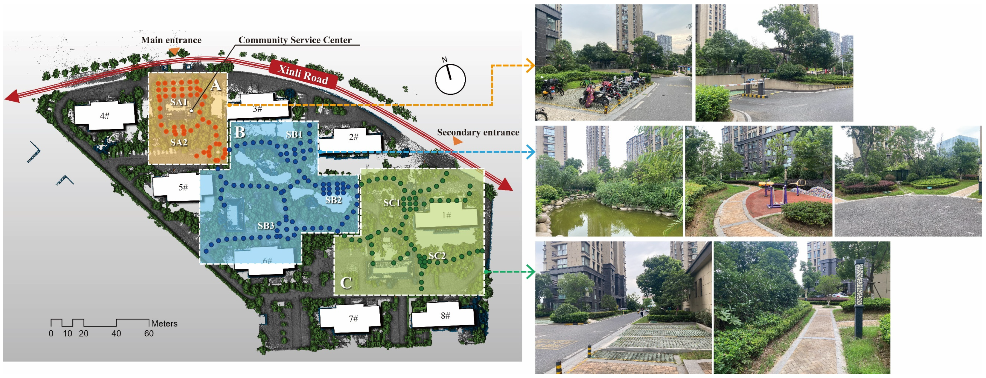
Aifei residential community (ARC) is located in Pukou District (Nanjing, China), north of Lixin Road, and was completed around 2017. It comprises 15 residential buildings with approximately 800 households. The internal building stock is predominantly high-rise. There are 8 buildings in ARC with 22–26 stories (Figure 1), considered as a dense residential area. The site area is about 75,777.5 m², and the total building floor area is about 19,497.3 m². The building coverage is approximately 22%, and the greening coverage is about 40%.

To characterize pedestrian-level visibility in a high-rise residential compound, viewpoints were sampled every 5 m along road centerlines, along plaza edges, and within plaza interiors, for a total of 223 viewpoints. In areas where finer detail was needed to represent walkable space, the spacing was locally reduced below 5 m. A 5-m step is sufficiently fine-grained to register significant alterations in the visual field caused by urban elements [40]. The viewpoints were elevated by 1.6 m above the ground surface to simulate eye height.

Preliminary on-site surveys show that the ARC residential landscape consists of three zones (Figure 2), each offering open areas for outdoor activities with distinct spatial characteristics. Zone A is the activity space near the main entrance. The main plaza is located to the north of the community service center, and the internal road loops around this center. The entire zone is shaded by relatively abundant vegetation. Zone B constitutes the main internal landscape, centered on small plazas, garden paths, and a central pond, with relatively dense planting. Zone C is the open space on the southeast side ARC, north of Buildings 7 and 8, characterized by broad roads and plazas with comparatively abundant vegetation. A total of 223 viewpoints were assigned to the three zones. Zone B contained the largest number of viewpoints, with 95 points (42.60%); Zone A contained the fewest, with 54 points (24.22%); and Zone C contained 74 points (33.18%). There are seven squares in ARC, designated according to the zoning as SA1 and SA2 in Zone A, SB1, SB2, and SB3 in Zone B, and SC1 and SC2 in Zone C.

2.2. Resident Questionnaire Survey

This study administered a structured questionnaire to assess residents’ perceptions and use of outdoor spaces in a high-density residential community. The full questionnaire is provided in Appendix A.1. The instrument comprised two sections with 10 questions: (i) basic demographics (4 questions) and (ii) evaluations of outdoor space quality and health-related experiences (6 questions). The second section included items on preferred outdoor activities, typical time of day, visit frequency, and duration, perceived importance of outdoor spaces for mental and physical restoration, recent experiential outcomes, including stress relief, increased energy, improved sleep, and location preferences within three mapped zones (A, B, C). Respondents also identified perceived environmental features of the outdoor spaces, for instance, vegetation richness, seating availability, spaciousness, quietness, privacy, etc. All items used closed-ended response formats with single- or multiple-choice options and clearly defined time bands. The instrument was developed based on prior literature on restorative environments and urban outdoor activity, then adapted to the local context through site reconnaissance and pilot checks. We collected 310 questionnaires. To reduce selection bias, the initial sample balanced sex with 155 men and 155 women, and more than 90% participants are adults. After preliminary screening and data cleaning, 279 questionnaires (90%) were deemed valid.

2.3. Hybrid-Model-Based Visibility Analysis

A hybrid spatial model integrating voxelized point clouds and solid 3D models (including terrain surface, water body, and buildings) is applied in this study [38]. The visibility analysis was conducted in ArcGIS Pro (version 3.3.0) for the solid models and in Python (3.11.7) for the point-cloud data.

2.3.1. LiDAR Point Cloud Collection and Voxelization

The point cloud data were acquired using a ZEB-HORIZON handheld 3D laser scanner (GeoSLAM, Nottingham, UK). For a fuller assessment of how residential greenery influences people, data collection was conducted in summer when vegetation is most developed. The raw point cloud contained all scene information and was classified into ground, vegetation, buildings, and other objects on Trimble Realworks with auto and manual classification. The original data were stored in LAZ format, with a file size of about 2.52 GB and approximately 1.358 billion points in total, of which vegetation points accounted for about 1.194 billion. The positional accuracy was approximately 1 cm. Vegetation points were extracted and converted into 100 mm voxels; after voxelization, the vegetation dataset was reduced to 493 MB (LAZ) with 15,263,664 points. Ground points were used to generate the digital elevation model (DEM), and building footprints were extracted from the point-cloud outlines of individual buildings.

2.3.2. 3D Hybrid Model Construction

The hybrid model in this study is composed of a solid model and a voxel model of vegetation point clouds. The solid model built consists of DEM, building masses, and water surfaces. As described in Section 2.3.1, we voxelized the vegetation points at a resolution of 100 mm, so that the resulting vegetation voxel model could better represent canopy volume and occlusion relationships. Using a 3D hybrid model for visibility analysis in high-density urban areas not only takes full advantage of the detailed information in point cloud data, but also helps overcome some LiDAR acquisition limitations, such as missing information on surfaces that laser beams penetrate or poorly capture, including water and glass.

As shown in Figure 3, we constructed the hybrid model in four steps. First, we classified the point cloud in Trimble RealWorks 10.4 using automatic processing with manual editing, assigning points to buildings, ground, vegetation, and others. Second, we removed non-target objects such as parked vehicles and pedestrians. Third, ground points were used to generate the terrain DEM, while building points were used to extract the footprint and maximum height of each building based on classified point clouds. Because the original point clouds were relatively sparse in upper stories and often missed façade details such as windows, we extruded the building footprints in ArcGIS Pro to create continuous 3D building blocks, compensating for those gaps. At the same time, we verified the water boundaries in Zone B through field surveys and satellite imagery, and created a corresponding 3D multipatch in ArcGIS Pro to represent the water surface. Finally, the DEM, building blocks, and water surface formed the solid model, which we overlaid with the voxelized vegetation model to produce the complete 3D hybrid scene for subsequent visibility analysis.

2.3.3. Line-of-Sight Analysis

Viewpoint locations were first defined and set to eye level (1.6 m), as described in Section 2.1. Human vision was simulated with a 360° horizontal field of view and a vertical field of view from −30° to 60° (0° = eye plane), as depicted in Figure 4a. From each viewpoint, a spherical set of 3D rays was generated with a maximum line-of-sight (LoS) length of 100 m (Figure 4b). The angular step was 3° in both azimuth and elevation, so each viewpoint produced 3388 rays. These rays discretize the pedestrian visual field and serve as “pixels” for computing visual perception indicators and for visualizing the scene.

Restricting the vertical range reduces low-value ground hits and aligns the simulated view with natural perception. The 3° sampling was chosen to balance computational load and the ability to capture fine elements such as tree canopies and building edges. All visibility computations were run in a single Python (v3.12) workflow. ArcGIS Pro was invoked through the arcpy library to perform LoS analysis on the solid model (Figure 4c). The resulting visible rays were then rechecked in Python against the vegetation voxel model with a size of 100 mm. Using 100 mm voxels provides sufficiently accurate estimates within tree canopies. [41]. If a ray intersected a voxel first, it was marked as blocked by vegetation and the hit point was recorded.

In the analysis, the object type at the first ray–object intersection is recorded. In other words, the feature that blocks the line of sight is stored as an attribute of that ray, so it can be used later for computing the visual exposure indicators. And any ray that encounters no obstruction within the set range is classified as sky.

2.3.4. Visual Perception Indicators

To characterize how residents perceive outdoor space in a dense residential compound, three visual perception indicators were defined at the pedestrian level. Based on the literature review in Section 1, SVF and GVF are considered important indices relating to human perception. Therefore, these two indicators are considered in this study. Besides, for fully using the advantage of point cloud data, a spatial indicator is proposed for evaluating the visual enclosure [42], which is hard to compute in 2D images. Each indicator is calculated from the classified first-hit results of the LoS rays, so every value directly reflects what a person standing at that viewpoint is most likely to see. Furthermore, temporary objects such as parked vehicles and moving pedestrians were identified as noise and removed, so that the indicators reflect stable built and vegetated structures.

(1)

Sky View Factor (SVF)

SVF is the proportion of the sky hemisphere visible from a given point near the ground and a standard descriptor of openness/enclosure at the pedestrian level [9,43]. In this study, it can be measured as the proportion of rays that reach the sky without being blocked. It is computed as

$$\mathrm{SVF}={\displaystyle \frac{N_{\mathit{sky}}}{N_{\mathit{total}}}}$$

(1)

where $N_{total}$ is the total number of LoS rays generated from a viewpoint, which equals 3388 in this case; $N_{sky}$ is the number of rays unobstructed by any object, which terminate at the sky. A higher SVF indicates a more open, less enclosed space, which is often associated with better daylight access and a weaker sense of confinement. In dense estates, SVF helps distinguish between highly enclosed courtyard spaces and more open plazas or road corridors.

(2)

Green View Factor (GVF)

In urban studies, GVF (or green view index, GVI) is a common concept. It quantifies the proportion of a pedestrian’s visual field occupied by vegetation [22,44]. Conceptually, it is the share of the observable scene covered by green elements (trees, shrubs, lawns). GVF ranges from 0 to 1 and reflects perceived greenness. It is calculated as

$$\mathrm{GVF}={\displaystyle \frac{N_{\mathit{green}}}{N_{\mathit{total}}}}$$

(2)

where $N_{Green}$ is the number of rays intercepted by vegetation. Higher GVF values mean that trees, shrubs, or other green elements are closer to the observer or occupy a larger part of the view. GVF is useful for identifying places with stronger biophilic qualities and for comparing how planting layouts affect perceived greenness.

(3)

Average Green Distance (AGD)

To measure the degree of green enclosure, we introduce Average Green Distance (AGD), a 3D visibility metric that captures the average distance between the viewpoint and all vegetation intercepted by first-hit rays. While GVF reflects “how much” greenery is visible, AGD reflects “how near” that greenery is. It is defined as

$$\mathrm{AGD}={\displaystyle \frac{1}{N_{\mathit{green}}}}\sum _{i=1}^{N_{\mathit{green}}}{l}_i$$

(3)

where $l_i$ denotes the length of the $i$-th ray that terminates at vegetation, that is, the distance between the viewpoint and the vegetation voxel that blocks the line of sight. A smaller AGD means vegetation is distributed closer to the observer and produces a stronger sense of green enclosure. This indicator compensates for the limitation of purely percentage-based metrics, which cannot distinguish near greenery from far greenery.

2.4. Statistical Analysis

Three spatial zones (Zone A, Zone B, and Zone C) were delineated a priori on the basis of field investigation, observed activity patterns, and the current functional organization of the site. These zones represent empirically defined usage areas, and the subsequent statistical analysis was intended to examine whether they also differ in terms of visual perception indicators.

Spearman correlation analysis was applied to investigate the relationship among three indicators. For each usage-based zone, descriptive statistics (mean, standard deviation, and number) were first calculated for the three visual indicators. Group differences were examined using a t-test and one-way analysis of variance (ANOVA). When the ANOVA indicated a significant overall effect (p < 0.05), pairwise comparisons between zones were performed using two-sample t-tests. To assess the magnitude of the observed differences, eta squared (η²) was computed for each ANOVA as the sum of squares between groups (SSB) divided by the total sum of squares (SST), representing the proportion of variance in the indicator explained by the zoning scheme. Following Cohen [45], η² values of approximately 0.01, 0.06, and 0.14 were interpreted as small, medium, and large effects, respectively. All statistical analyses were performed in R (version 4.5.2). The significance level was set at $p=0.05$, and statistical significance was reported as *$p<0.05$, **$p<0.01$, and ***$p<0.001$.

3. Results

3.1. Residential Landscape Preference

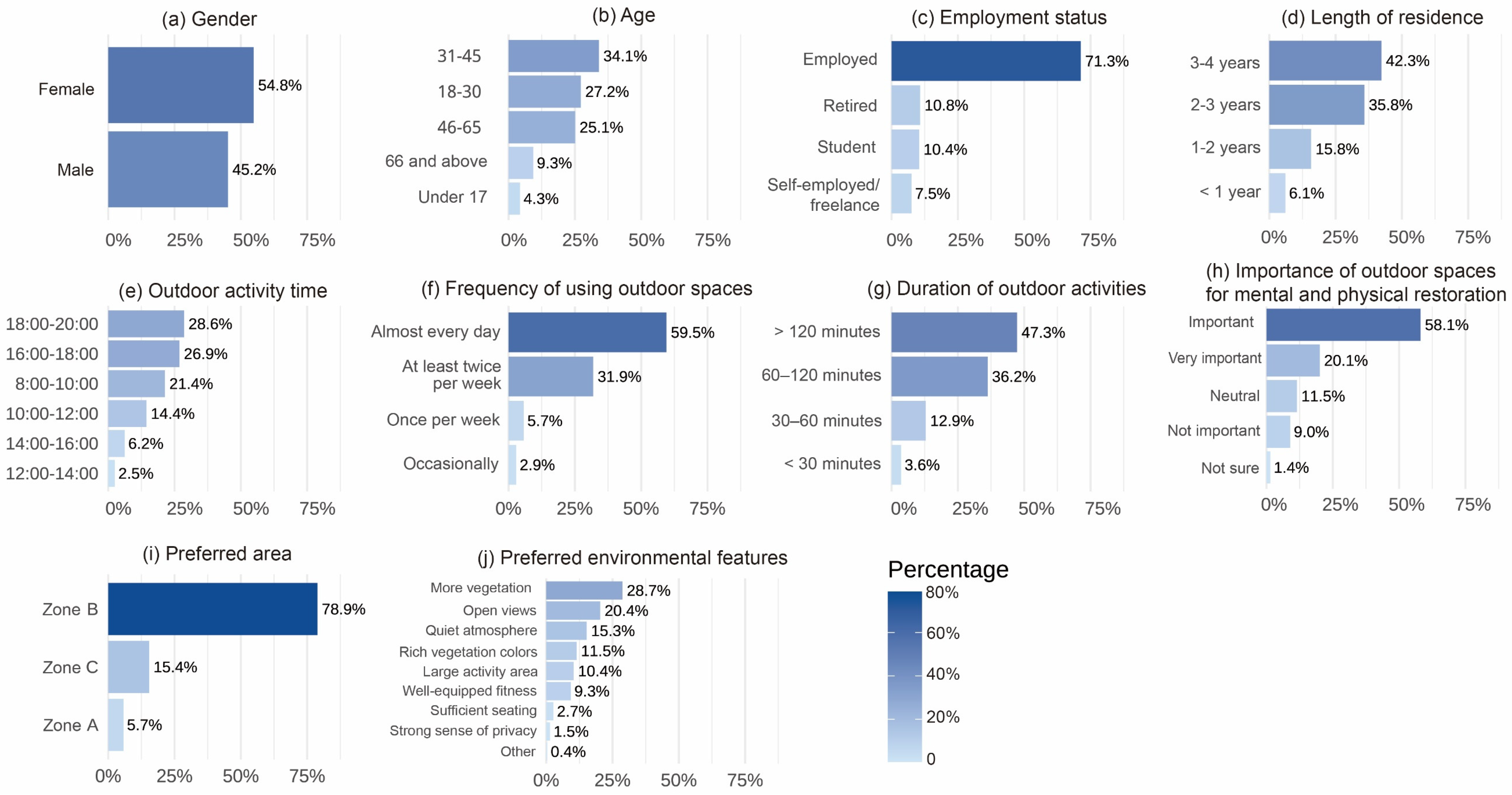
We randomly sampled 310 residents living in ARC, each from a different household. To base evaluations on substantial first-hand experience and enhance ecological validity, the questionnaire was distributed to long-term residents of the study area, over 94% of whom had resided there for more than one year (Figure 5d). A total of 310 questionnaires were distributed and collected, of which 279 were valid (90%). The descriptive statistics of 279 questionnaires reveal a relatively homogeneous and active user group (Appendix A.2). Survey-based profiles of users and their outdoor spatial preferences can be found in Figure 5. Females slightly outnumber males, and most respondents are working-age adults, with the largest share in the 31–45 group, followed by 18–30 and 46–65 years.

From Figure 5f,g, it is clear that the residential outdoor space is a primary place for daily activities. Nearly 60% of respondents reported going outdoors almost every day in the community, and 47.3% stayed outside for 1–2 h each time. Importantly, outdoor space is widely regarded as restorative. It is reported that close to 80% rated it as “important” or “very important” for mental and physical recovery. These items together show that residential outdoor spaces are both frequently used and regarded as highly important by residents.

A clear spatial preference emerges. Among the three activity zones, Zone B was overwhelmingly preferred at nearly 80%, Zone C received a moderate share, and Zone A was chosen by only a small number of users. Preference for environmental features further supports this interpretation: respondents most often selected items such as “more vegetation” and “open view,” while more detailed or facility-oriented attributes were chosen less frequently.

3.2. Mapping Visual Perception Indicators

In the calculation, six outliers were identified. At these viewpoints, the rays were completely wrapped by vegetation voxels, resulting in SVF = 0, GVF = 1, and AGD < 0.1 m. These points represent highly occluded edge positions that are not typical of general pedestrian viewpoints, and removing them prevents distortion of the descriptive statistics while exerting only a minor influence on the overall patterns reported in the Results. After removing these points, 217 valid viewpoints remained. Figure 6 illustrates the spatial pattern of the three visual perception indicators along the walking routes, and the descriptive statistics (

Table 1. Descriptive statistics of visual perception indicators by zone.

Indicator	Value	Zone A (n = 54)	Zone B (n = 90)	Zone C (n = 73)	Total (n = 217)
SVF	Min	0.005	0.007	0.002	0.002
	Max	0.357	0.378	0.321	0.378
	mean (SD)	0.127 (0.091)	0.162 (0.058)	0.131 (0.068)	0.143 (0.072)
GVF	Min	0.016	0.083	0.093	0.016
	Max	0.931	0.924	0.906	0.931
	mean (SD)	0.598 (0.241)	0.507 (0.173)	0.524 (0.200)	0.535 (0.203)
AGD	Min	1.370	1.033	0.519	0.519
	Max	11.395	13.785	17.721	17.721
	mean (SD)	5.380 (2.430)	6.810 (3.010)	6.600 (3.010)	6.380 (2.923)

Note: SD = standard deviation. Bold values indicate the highest mean within each row.

) confirm that the three usage-based zones correspond to different visual–spatial conditions. Focusing on the square spaces across the three zones, most of them exhibit a common pattern of relatively high SVF and low GVF, indicating generally open views with limited close-range greenery. This is especially true for SB2 and SB3, where vegetation is set back from the main activity area, resulting in better openness and a stronger sense of spatial freedom. In contrast, SB1 in Zone B shows more moderate values of SVF, GVF, and AGD, suggesting that Zone B contains a mix of square types and thus offers more diverse spatial experiences.

SVF values are mainly higher along the central and eastern paths, which are largely located in Zone B. This is consistent with the statistics: Zone B records the highest mean SVF (0.162 ± 0.058), whereas Zone A (0.127 ± 0.091) and Zone C (0.131 ± 0.068) show lower and very similar averages. Zone B also reaches the global maximum (0.378), indicating that this zone contains the most open viewpoints with limited vertical obstruction. The larger SD in Zone A suggests that this zone mixes locally open and locally shaded segments.

The GVF map shows an almost opposite pattern. High green visibility is concentrated in the northern and inner landscaped strips, which are mainly assigned to Zone A. Zone A has the highest mean GVF (0.598 ± 0.241) and also the overall maximum (0.931), meaning some viewpoints are strongly enclosed by vegetation. Zone B has the lowest mean GVF (0.507 ± 0.173), and Zone C is intermediate (0.524 ± 0.200), indicating that Zones B and C are visually less dominated by vegetation than Zone A. According to previous studies, a GVF greater than 0.35 is already considered very high [46,47]. In our case, the GVF across the entire study area exceeds 0.50, indicating that the ARC residential community is highly and uniformly greened.

AGD is greater along the southern belt and parts of the central route, corresponding mainly to Zones B and C. Statistically, Zone B shows the largest mean AGD (6.81 ± 3.01 m), followed by Zone C (6.60 ± 3.01 m), while Zone A has the smallest value (5.38 ± 2.43 m). Since a larger AGD means that vegetation is, on average, farther away from the viewpoint, this pattern confirms that Zones B and C are visually more open toward surrounding greenery, whereas Zone A is closer to, and more frequently surrounded by, vegetation.

Overall, the spatial maps and numerical summaries tell a coherent story: Zone B represents the most open visual environment, Zone A represents a vegetation-enclosed environment, and Zone C functions as an intermediate type that shares part of the openness of Zone B but does not reach its sky visibility. This spatial–numerical consistency supports the validity of the usage-based zoning.

3.3. Differences of Visual Perception Indicator Between Zones

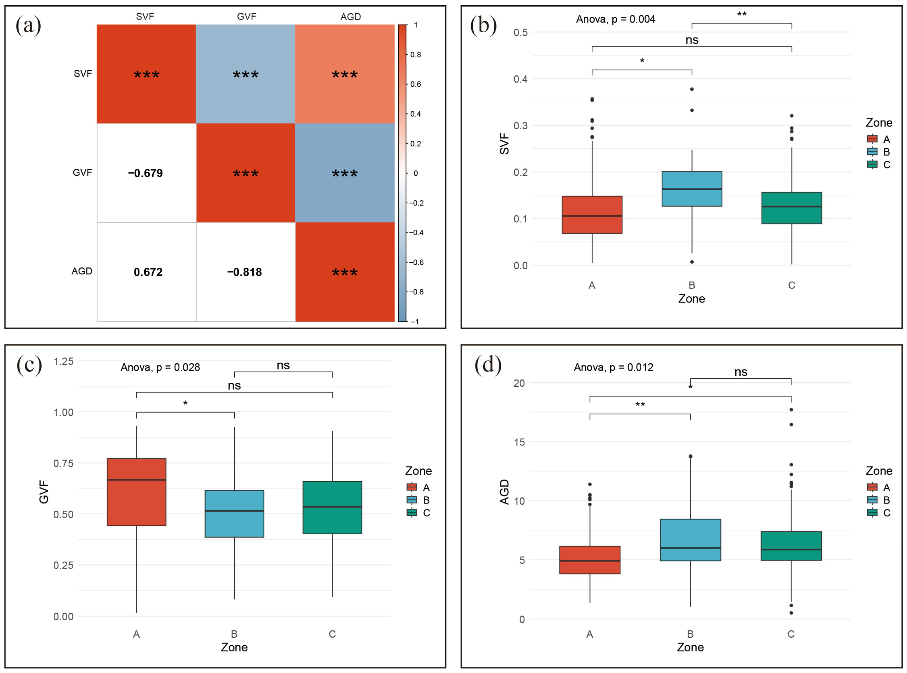
The results show that the empirically defined zones are also statistically distinguishable in terms of visual perception. As illustrated in Figure 7a, the three indicators are strongly and systematically related. SVF is negatively correlated with GVF and positively correlated with AGD, while GVF is strongly and negatively correlated with AGD (all p < 0.001). This pattern is consistent with actual spatial visual experience: the way vegetation is arranged directly affects how large or enclosed a space feels. When vegetation is dense and located close to the observer, GVF tends to be high, while SVF and AGD are correspondingly low. This confirms that the indicators jointly describe an openness–enclosure gradient, where high sky visibility coincides with low green enclosure and vegetation located farther from the viewpoint.

When this gradient is examined by zone (Figure 7b–d), clear distributional differences emerge. Zone B tends to occupy the more visually open space of the distribution, showing higher SVF and larger AGD, whereas Zone A is characterized by higher GVF and shorter AGD, indicating a vegetation-enclosed condition. Zone C generally lies between the other two zones. Pairwise t-tests displayed on the boxplots further clarified the differences between zones. The open-use zone (Zone B) had significantly higher SVF and greater vegetation distance than at least one of the other zones, while the vegetation-dominated zone (Zone A) had significantly higher GVF than Zone B. Together, these results demonstrate that the field-based zoning is consistent with quantitative visual perception measures and that the three indicators converge to describe the same spatial structure.

These visual patterns are supported by the one-way ANOVA (

Table 2. One-way ANOVA results for visual perception indicators.

Indicator	SSB	SST	F	p-Value	η2 = SSB/SST
SVF	0.057	1.132	5.668	0.004	0.050
GVF	0.293	8.902	3.639	0.028	0.033
AGD	74.515	1845.492	4.502	0.012	0.040

). SVF, GVF, and AGD all differed significantly among zones. The corresponding effect sizes were small to moderate (η² = 0.033–0.050), meaning that the zoning scheme explains about 3–5% of the variance in these indicators. Overall, the ANOVA results and the patterns in Figure 6 show that the three zones differ in both behavior and visual form. Zone B is the most open. Zone A is more enclosed by vegetation. Zone C falls in between.

4. Discussion

4.1. Implications and Potential Applications

This study combined street-level visual indicators with on-site behavioral data to test whether usage-based zoning in a high-density residential compound is also legible in visual–spatial terms. Methodologically, three layers of analysis were integrated: (1) objective indicators derived at viewpoint level, sky view factor (SVF), green view factor (GVF), and average green distance (AGD), which together describe an openness–enclosure gradient similar to what has been reported for visual greenery and perceived comfort in residential settings [26,48]; (2) statistical tests to verify whether the three empirically defined zones differ in these indicators; and (3) a resident survey that profiled users’ socio-demographics, outdoor-use patterns, and preferences for zones and environmental features. This mixed strategy allowed us to link what space looks like to how it is actually chosen and used.

Taken together, survey results with visibility analysis results, a clear spatial preference emerges. Based on the results, we found that all three indicators differed significantly among zones, with small-to-moderate effect sizes, and the most open zone (Zone B) was also the most preferred one. Regular users tend to choose outdoor spaces that offer both greenery and good visual openness, and under the current layout Zone B fits this condition best. Among the three activity zones, about 79% of respondents preferred Zone B, while Zone C received a moderate share and Zone A was selected by only a few users. This pattern is consistent with the visual–spatial analysis, which shows that Zone B provides a more open and comfortable environment. Zone B scored higher in SVF and AGD and lower in GVF, which offered a more spacious, visually permeable setting with vegetation. The evidence does not support H1 or H2 in this context. However, this configuration aligns well with residents’ stated preferences for “open view” and with restorative-environment theory, which argues that visual access, depth, and moderate natural elements support restoration and lingering [49,50]. In this study, Average Green Distance (AGD) emerges as a key predictor of resident preference—an eye-level proximity metric that image-based approaches cannot readily quantify. Our finding echoes Saadativaghar et al., who reported that the indirect effect of vegetational variables on restoration through the mediator variable of being away was confirmed [51], consistent with attention-restoration pathways. In short, the findings imply that not only how much greenery is visible (measured by GVF), but also how far it sits from the observer, helps explain preference.

By contrast, Zone A showed the opposite visual signature, higher GVF, lower SVF, shorter green distance, corresponding to a more vegetated but more enclosed experience, and it was chosen far less often in the survey. Although 28.73% of respondents said they prefer outdoor spaces with more vegetation, our analysis shows that Zone A, with the highest GVF, was the least preferred. The finding implies that “more green” is not generally preferable, which accords with earlier work showing a negative relationship between GVF and Physiological Equivalent Temperature (PET) [52]. When vegetation becomes too dense and too close, it can create excessive visual enclosure and even block desired views, which in turn reduces people’s willingness to use this space. Only 1.5% of residents preferred more private, highly enclosed spaces. This suggests that most residents do not want outdoor areas in the community to be too closed. Zone A shows the lowest AGD, which means vegetation is very close to the viewpoints and the space is more enclosed. This may explain why Zone A was the least frequently chosen. Zone C, with intermediate values, also attracted intermediate levels of preference.

For high-density residential environments, there are two practical implications. First, not all outdoor space has to be equally greened; what users rewarded here was structured openness with accessible greenery, not maximal enclosure. Designers and managers can therefore purposefully reserve some circulation spines or central lawns as high-SVF, long-distance views, while locating denser planting, seats, or semi-private corners in secondary zones. Second, residents of different ages may prefer different types of outdoor spaces. Design strategies can therefore be tailored to specific age groups to create an age-friendly residential outdoor environment. For example, open, view-rich areas for everyday, cross-age use, and more vegetated, sheltered pockets for older or quieter users, echoing age-sensitive open-space recommendations in dense Asian residential areas [53,54]. This suggests that viewpoint-level visual indicators are not only analytic tools but can be embedded in design guidelines to check whether planned spaces will reproduce the resident-favored pattern observed here.

4.2. Limitations and Future Work

At the same time, several limitations point to directions for further work. First, the present preference analysis was linked to administratively/empirically defined zones; in future studies, preferences could be mapped directly onto clusters derived from the visual perception indicators themselves. For instance, clustering viewpoints by SVF–GVF–AGD and then testing which clusters users favor. That would tell us whether people are responding to our planning units or to finer-grained visual patterns. Second, the indicator set was intentionally concise; high-density outdoor space could be described more fully by adding façade enclosure, ground permeability, or even semantic/image features, which would allow a more nuanced guidance for design. Third, our analysis draws on one residential community and a context of high density with ample greenery; these conditions may limit how broadly the results apply. Applying the same workflow to more cases with different building layouts, greening ratios, and resident profiles would help establish how generalizable the residence-favored pattern really is, and whether demographical context shifts the optimum.

Future studies will include seasonal variation in vegetation, with multi-season spatial and survey campaigns to better capture the spatiotemporal dimensions of residents’ green-space perception. While this study examined associations between outdoor greenery morphology and stated preferences, it did not unpack the underlying mechanisms. As a next step, we will test potential mediators, including microclimatic conditions (for instance, air radiant temperature and wind distribution) and environmental-psychology constructs (for instance, stress recovery, attention restoration and comfort), using mediation, structural equation or multilevel models to clarify how greenery shapes preference.

5. Conclusions

This study set out to verify whether a usage-based spatial subdivision in a high-density residential compound is also legible in quantitative visual terms, and whether such visual patterns are consistent with residents’ stated preferences. We combined three levels of evidence: (i) visual perception indicators, including sky view factor (SVF), green view factor (GVF), and average green distance (AGD), to describe an openness–enclosure gradient, following earlier work on street-level greenery and visual comfort; (ii) one-way ANOVA with effect sizes to test whether the three empirically defined zones actually differ; and (iii) a questionnaire capturing socio-demographics, outdoor-use rhythms, and preferences for zones and environmental features. This multi-source design made it possible to connect how spaces look, how they are structured, and what residents report they prefer. Based on the questionnaire and the quantitative visual analysis, this study found a preliminary preference pattern for outdoor space in high-density residential areas. When overall greening is high, residents tend to favor spaces with greater visual openness rather than spaces that are heavily wrapped by vegetation.

Beyond the case itself, the workflow we developed, integrating solid 3D models with voxelized LiDAR point clouds and linking them to resident survey data, offers a technical path that fits well with the vision of future, intelligent cities. It shows how fine-grained spatial data can be used to “see” urban space from the pedestrian’s perspective and to test design options digitally before implementation. Such data-driven visibility analysis can be embedded in smart planning platforms, support low-carbon community renewal by optimizing existing greenery instead of overplanting, and help reconfigure public interaction spaces, green courtyards, and linear parks to better serve health-oriented urban life. As cities move toward intelligent management, 3D scene reconstruction and point-cloud-based assessment can become routine tools for evaluating livability, micro-scale walkability, and visual comfort.

This study offers direct guidance for outdoor landscape design in high-density residential areas. The results suggest configuring vegetation with an appropriate setback from pedestrian paths so that people experience adequate openness while still perceiving greenery. Designers should avoid dense, close plantings that create excessive enclosure. The framework links 3D, pedestrian-level visual indicators to resident preference and helps identify spatial configurations that better meet user needs. It can support sustainable urban planning and smart-city workflows by testing planting layouts, spatial configuration for greenery, and view management before implementation. In this sense, the proposed framework is not only a method for one residential community, but also a transferable component for future-city toolkits to identify urban spatial morphologies that better meet people’s needs, supporting sustainable land use, healthy-city goals, and human-centered urban renewal in increasingly dense environments.

References

1. Bai, X.; Shi, P. China’s urbanization at a turning point—Challenges and opportunities. Science 2025, 388, eadw3443. [Google Scholar] [CrossRef] [PubMed]
2. Wang, F.; Liu, S.; Chen, T.; Zhang, H.; Zhang, Y.; Bai, X. How urbanization affects residents’ health risks: Evidence from China. Environ. Sci. Pollut. Res. 2023, 30, 35554–35571. [Google Scholar] [CrossRef] [PubMed]
3. Liu, Z.; Chen, X.; Cui, H.; Ma, Y.; Gao, N.; Li, X.; Meng, X.; Lin, H.; Abudou, H.; Guo, L.; et al. Green space exposure on depression and anxiety outcomes: A meta-analysis. Environ. Res. 2023, 231, 116303. [Google Scholar] [CrossRef] [PubMed]
4. Ventriglio, A.; Torales, J.; Castaldelli-Maia, J.M.; De Berardis, D.; Bhugra, D. Urbanization and emerging mental health issues. CNS Spectr. 2021, 26, 43–50. [Google Scholar] [CrossRef]
5. Huang, W.; Lin, G. The relationship between urban green space and social health of individuals: A scoping review. Urban For. Urban Green. 2023, 85, 127969. [Google Scholar] [CrossRef]
6. He, D.; Miao, J.; Lu, Y.; Song, Y.; Chen, L.; Liu, Y. Urban greenery mitigates the negative effect of urban density on older adults’ life satisfaction: Evidence from Shanghai, China. Cities 2022, 124, 103607. [Google Scholar] [CrossRef]
7. Peng, Z.; Bardhan, R.; Ellard, C.; Steemers, K. Urban climate walk: A stop-and-go assessment of the dynamic thermal sensation and perception in two waterfront districts in Rome, Italy. Build. Environ. 2022, 221, 109267. [Google Scholar] [CrossRef]
8. Zhang, S.; Zhao, X.; Zeng, Z.; Qiu, X. The Influence of Audio-Visual Interactions on Psychological Responses of Young People in Urban Green Areas: A Case Study in Two Parks in China. Int. J. Environ. Res. Public Health 2019, 16, 1845. [Google Scholar] [CrossRef]
9. Junsik, K.; Dong-Kun, L.; Robert, D.B.; Saehoon, K.; Jun-Hyun, K.; Sunyong, S. The effect of extremely low sky view factor on land surface temperatures in urban residential areas. Sustain. Cities Soc. 2022, 80, 103799. [Google Scholar] [CrossRef]
10. Xiong, W.; Wu, Q.; Qi, J.; Li, J.; Zhu, S.; Qiu, B. Spatiotemporal dynamics of land surface temperature and its drivers within the local climate zone framework. Sustain. Cities Soc. 2025, 133, 106859. [Google Scholar] [CrossRef]
11. Gao, S.; Ma, Y.; Wang, C.; Xue, H.; Zhu, K.; Hou, S.; Feng, C. Assessing urban greenery impact on human psychological and physiological responses through virtual reality. Build. Environ. 2025, 272, 112696. [Google Scholar] [CrossRef]
12. Macintyre, V.G.; Cotterill, S.; Anderson, J.; Phillipson, C.; Benton, J.S.; French, D.P. “I Would Never Come Here Because I’ve Got My Own Garden”: Older Adults’ Perceptions of Small Urban Green Spaces. Int. J. Environ. Res. Public Health 2019, 16, 1994. [Google Scholar] [CrossRef]
13. Elsadek, M.; Sun, M.; Sugiyama, R.; Fujii, E. Cross-cultural comparison of physiological and psychological responses to different garden styles. Urban For. Urban Green. 2019, 38, 74–83. [Google Scholar] [CrossRef]
14. Schmidt, T.; Kerr, J.; Schipperijn, J. Associations between Neighborhood Open Space Features and Walking and Social Interaction in Older Adults-A Mixed Methods Study. Geriatrics 2019, 4, 41. [Google Scholar] [CrossRef] [PubMed]
15. Mohr-Stockinger, S.; Sanft, S.J.; Büttner, F.; Butenschön, S.; Rennert, R.; Säumel, I. Awakening the sleeping giant of urban green in times of crisis-coverage, co-creation and practical guidelines for optimizing biodiversity-friendly and health-promoting residential greenery. Front. Public Health 2023, 11, 14. [Google Scholar] [CrossRef] [PubMed]
16. Aerts, R.; Vanlessen, N.; Dujardin, S.; Nemery, B.; Van Nieuwenhuyse, A.; Bauwelinck, M.; Casas, L.; Demoury, C.; Plusquin, M.; Nawrot, T.S. Residential green space and mental health-related prescription medication sales: An ecological study in Belgium. Environ. Res. 2022, 211, 8. [Google Scholar] [CrossRef]
17. Kang, Y.; Kim, E.J. Differences of Restorative Effects While Viewing Urban Landscapes and Green Landscapes. Sustainability 2019, 11, 2129. [Google Scholar] [CrossRef]
18. Krekel, C.; Kolbe, J.; Wüstemann, H. The greener, the happier? The effect of urban land use on residential well-being. Ecol. Econ. 2016, 121, 117–127. [Google Scholar] [CrossRef]
19. Chen, K.; Zhang, T.; Liu, F.; Zhang, Y.; Song, Y. How Does Urban Green Space Impact Residents’ Mental Health: A Literature Review of Mediators. Int. J. Environ. Res. Public Health 2021, 18, 11746. [Google Scholar] [CrossRef]
20. Bahr, S. The relationship between urban greenery, mixed land use and life satisfaction: An examination using remote sensing data and deep learning. Landsc. Urban Plan. 2024, 251, 105174. [Google Scholar] [CrossRef]
21. Martinez, A.d.l.I.; Labib, S.M. Demystifying normalized difference vegetation index (NDVI) for greenness exposure assessments and policy interventions in urban greening. Environ. Res. 2023, 220, 115155. [Google Scholar] [CrossRef]
22. Zhu, H.; Nan, X.; Yang, F.; Bao, Z. Utilizing the green view index to improve the urban street greenery index system: A statistical study using road patterns and vegetation structures as entry points. Landsc. Urban Plan. 2023, 237, 104780. [Google Scholar] [CrossRef]
23. Ren, Z.; Du, Y.; He, X.; Pu, R.; Zheng, H.; Hu, H. Spatiotemporal pattern of urban forest leaf area index in response to rapid urbanization and urban greening. J. For. Res. 2018, 29, 785–796. [Google Scholar] [CrossRef]
24. Pettorelli, N.; Vik, J.O.; Mysterud, A.; Gaillard, J.-M.; Tucker, C.J.; Stenseth, N.C. Using the satellite-derived NDVI to assess ecological responses to environmental change. Trends Ecol. Evol. 2005, 20, 503–510. [Google Scholar] [CrossRef] [PubMed]
25. Susaki, J.; Kubota, S. Automatic Assessment of Green Space Ratio in Urban Areas from Mobile Scanning Data. Remote Sens. 2017, 9, 215. [Google Scholar] [CrossRef]
26. Li, X.; Zhang, C.; Li, W.; Ricard, R.; Meng, Q.; Zhang, W. Assessing street-level urban greenery using Google Street View and a modified green view index. Urban For. Urban Green. 2015, 14, 675–685. [Google Scholar] [CrossRef]
27. Herbert, G.; Chen, X. A comparison of usefulness of 2D and 3D representations of urban planning. Cartogr. Geogr. Inf. Sci. 2015, 42, 22–32. [Google Scholar] [CrossRef]
28. Wu, B.; Yu, B.; Shu, S.; Liang, H.; Zhao, Y.; Wu, J. Mapping fine-scale visual quality distribution inside urban streets using mobile LiDAR data. Build. Environ. 2021, 206, 108323. [Google Scholar] [CrossRef]
29. Zhou, L.; Li, X.; Zhang, B.; Xuan, J.; Gong, Y.; Tan, C.; Huang, H.; Du, H. Estimating 3D Green Volume and Aboveground Biomass of Urban Forest Trees by UAV-Lidar. Remote Sens. 2022, 14, 5211. [Google Scholar] [CrossRef]
30. Urech, P.R.; Dissegna, M.A.; Girot, C.; Grêt-Regamey, A. Point cloud modeling as a bridge between landscape design and planning. Landsc. Urban Plan. 2020, 203, 103903. [Google Scholar] [CrossRef]
31. Jaalama, K.; Kauhanen, H.; Keitaanniemi, A.; Rantanen, T.; Virtanen, J.-P.; Julin, A.; Vaaja, M.; Ingman, M.; Ahlavuo, M.; Hyyppä, H. 3D Point Cloud Data in Conveying Information for Local Green Factor Assessment. ISPRS Int. J. Geo-Inf. 2021, 10, 762. [Google Scholar] [CrossRef]
32. Weinmann, M.; Urban, S.; Hinz, S.; Jutzi, B.; Mallet, C. Distinctive 2D and 3D features for automated large-scale scene analysis in urban areas. Comput. Graph. 2015, 49, 47–57. [Google Scholar] [CrossRef]
33. Zhao, Y.; Wu, B.; Wu, J.; Shu, S.; Liang, H.; Liu, M.; Badenko, V.; Fedotov, A.; Yao, S.; Yu, B. Mapping 3D visibility in an urban street environment from mobile LiDAR point clouds. GIScience Remote Sens. 2020, 57, 797–812. [Google Scholar] [CrossRef]
34. Münzinger, M.; Prechtel, N.; Behnisch, M. Mapping the Urban forest in detail: From LiDAR point clouds to 3D tree models. Urban For. Urban Green. 2022, 74, 127637. [Google Scholar] [CrossRef]
35. Zhang, G.; Verbree, E.; Wang, X. An Approach to Map Visibility in the Built Environment From Airborne LiDAR Point Clouds. IEEE Access 2021, 9, 44150–44161. [Google Scholar] [CrossRef]
36. Liu, X.; Li, J.; Nazeer, M.; Wong, M.S. Advanced point cloud completion for urban trees: A novel approach using enhanced SnowflakeNet. Urban For. Urban Green. 2025, 113, 129107. [Google Scholar] [CrossRef]
37. Klingberg, J.; Konarska, J.; Lindberg, F.; Johansson, L.; Thorsson, S. Mapping leaf area of urban greenery using aerial LiDAR and ground-based measurements in Gothenburg, Sweden. Urban For. Urban Green. 2017, 26, 31–40. [Google Scholar] [CrossRef]
38. Zhang, G.; Yang, D.; Cheng, S. Voxelized Point Cloud and Solid 3D Model Integration to Assess Visual Exposure in Yueya Lake Park, Nanjing. Land 2025, 14, 2095. [Google Scholar] [CrossRef]
39. Orozco Carpio, P.R.; Viñals, M.J.; López-González, M.C. 3D Point Cloud and GIS Approach to Assess Street Physical Attributes. Smart Cities 2024, 7, 991–1006. [Google Scholar] [CrossRef]
40. Benedikt, M.L. To take hold of space: Isovists and isovist fields. Environ. Plan. B 1979, 6, 47–65. [Google Scholar] [CrossRef]
41. Zong, X.; Wang, T.; Skidmore, A.K.; Heurich, M. The impact of voxel size, forest type, and understory cover on visibility estimation in forests using terrestrial laser scanning. GIScience Remote Sens. 2021, 58, 323–339. [Google Scholar] [CrossRef]
42. Stamps, A.E. Isovists, enclosure, and permeability theory. Environ. Plan. B-Plan. Des. 2005, 32, 735–762. [Google Scholar] [CrossRef]
43. Liu, Y.; Yu, Z.; Song, Y.; Yu, X.; Zhang, J.; Song, D. Psychological influence of sky view factor and green view index on daytime thermal comfort of pedestrians in Shanghai. Urban Clim. 2024, 56, 102014. [Google Scholar] [CrossRef]
44. Yin, D.; Hirata, T. Comprehensive Comparative Analysis and Innovative Exploration of Green View Index Calculation Methods. Land 2025, 14, 289. [Google Scholar] [CrossRef]
45. Cohen, J. Statistical Power Analysis for the Behavioral Sciences; Routledge: New York, NY, USA, 2013. [Google Scholar]
46. Huang, J.; Liang, J.; Yang, M.; Li, Y. Visual Preference Analysis and Planning Responses Based on Street View Images: A Case Study of Gulangyu Island, China. Land 2023, 12, 129. [Google Scholar] [CrossRef]
47. Li, T.; Zheng, X.; Wu, J.; Zhang, Y.; Fu, X.; Deng, H. Spatial relationship between green view index and normalized differential vegetation index within the Sixth Ring Road of Beijing. Urban For. Urban Green. 2021, 62, 127153. [Google Scholar] [CrossRef]
48. Zhang, Y.; Dong, R. Impacts of Street-Visible Greenery on Housing Prices: Evidence from a Hedonic Price Model and a Massive Street View Image Dataset in Beijing. ISPRS Int. J. Geo-Inf. 2018, 7, 104. [Google Scholar] [CrossRef]
49. Ulrich, R.S. View through a window may influence recovery from surgery. Science 1984, 224, 420–421. [Google Scholar] [CrossRef]
50. Kaplan, R.; Kaplan, S. The Experience of Nature: A Psychological Perspective; Cambridge University Press: New York, NY, USA, 1989. [Google Scholar]
51. Saadativaghar, P.; Zarghami, E.; Ghanbaran, A. Measuring restoration likelihood of tall building scapes: Physical features and vegetation. Landsc. Ecol. Eng. 2024, 20, 363–395. [Google Scholar] [CrossRef]
52. Wang, Q.; Sun, W.; Tang, S.; Zhou, X. SVI-GVI integration for thermal comfort in urban parks: A case study of Changchun in cold regions. Theor. Appl. Climatol. 2025, 156, 318. [Google Scholar] [CrossRef]
53. Shao, Y.; Yin, Y.; Xue, Z.; Ma, D. Assessing and Comparing the Visual Comfort of Streets across Four Chinese Megacities Using AI-Based Image Analysis and the Perceptive Evaluation Method. Land 2023, 12, 834. [Google Scholar] [CrossRef]
54. Jim, C.Y.; Chan, M.W.H. Urban greenspace delivery in Hong Kong: Spatial-institutional limitations and solutions. Urban For. Urban Green. 2016, 18, 65–85. [Google Scholar] [CrossRef]
Figure 1. Study area and viewpoint allocation: Numbers 1#–8# denote the corresponding residential buildings.
Buildings 15 04275 g001
Figure 2. The three principal activity spaces in the Aifei residential community and corresponding status-quo photographs: Zone A is the main entrance and plaza area (SA1, SA2), broadly shaded; Zone B is the internal landscape with small plazas (SB1–SB3), garden paths, and a central pond, with denser planting; Zone C is the southeast open area with broad roads and plazas (SC1, SC2). Colored dots indicate viewpoints and match the zone legend.
Buildings 15 04275 g002
Figure 3. The workflow of 3D hybrid model construction. Step 1: Classify the point cloud; Step 2: Clean the classified points; Step 3: Build the solid model from ground and building points; Step 4: Build the vegetation voxel model and integrate both to form the hybrid model.
Buildings 15 04275 g003
Figure 4. Line-of-Sight analysis based on 3D hybrid model. (a) Hemispherical modeling of the human visual field; (b) 3D sight lines simulating pedestrian visual space; (c) calculation of visible sight lines on the solid model using the Line of Sight function in ArcGIS Pro; (d) refinement of visible sight lines with vegetation voxels based on the ArcGIS Pro results.
Buildings 15 04275 g004
Figure 5. Percentage distribution of questionnaire responses: (a) gender; (b) age; (c) employment status; (d) length of residence; (e) outdoor activity time; (f) frequency of using outdoor spaces; (g) duration of outdoor activities; (h) importance of outdoor spaces for mental and physical restoration; (i) preferred area; and (j) preferred environmental features.
Buildings 15 04275 g005
Figure 6. Spatial distribution of visual perception indicators along the pedestrian network. (a) Sky View Factor (SVF): higher values cluster in the squares (SA1, SB1, SB2), while lower values are mostly along the roads.; (b) Green View Factor (GVF): high values concentrate along the roads in Zone A; (c) Average Green Distance (AGD): squares in Zone B show the greatest distances to surrounding greenery.
Buildings 15 04275 g006
Figure 7. Statistical analysis of the three indicators: (a) Correlation heatmap showing a strong negative correlation between GVF and both SVF and AGD, and a positive correlation between SVF and AGD; (b) boxplots and t-test results for SVF, with Zone B showing the highest values and Zone A the lowest; (c) boxplots and t-test results for GVF, with Zone A having the highest values and Zones B and C at lower, similar levels; (d) boxplots and t-test results for AGD, with the shortest distances in Zone A and longer distances in Zones B and C, and significant differences between Zone A and the other two zones. Note: *   p < 0.05 , **   p < 0.01 , and ***   p < 0.001 .
Buildings 15 04275 g007