Article

Benchmarking Conventional Machine Learning Models for Dynamic Soil Property Prediction

1
Department of Civil and Environmental Engineering, College of Engineering, University of Sharjah, Sharjah P.O. Box 27272, United Arab Emirates
2
Structural Engineering Department, Mansoura University, Al-Gomhoria Street, Mansoura P.O. Box 35516, Egypt
3
Department of Public Health, School of Health Sciences and Psychology, Canadian University Dubai, Dubai P.O. Box 117781, United Arab Emirates
*
Author to whom correspondence should be addressed.
Buildings 2025, 15(22), 4188; https://doi.org/10.3390/buildings15224188
Submission received: 8 September 2025 / Revised: 18 October 2025 / Accepted: 24 October 2025 / Published: 19 November 2025
(This article belongs to the Special Issue Research on Intelligent Geotechnical Engineering)

Abstract

Reliable estimates of soil stiffness and energy dissipation are essential for dynamic-response design. This study benchmarks machine learning models for predicting shear modulus (G) and damping ratio (D) using 2738 resonant-column measurements. After data quality control and F-test feature screening, five model families—decision trees and ensembles, support-vector machines, Gaussian-process regression, neural networks, and linear baselines—were trained under uniform 10-fold cross-validation and evaluated with R2, RMSE, MAE, and MSE, while recording training time to reflect practical constraints. Results show that model choice materially affects performance. For G, a bagged ensemble of trees delivered the best accuracy (R2 = 0.9827) with short training times; single trees provided transparent, fast screening models. For D, tree-based ensembles again performed strongly (R2 up to 0.8565), while a rational-quadratic Gaussian-process model offered competitive accuracy (R2 ≈ 0.81) together with prediction intervals that support risk-aware design. Feature influence aligned with soil mechanics: G was most sensitive to effective confining pressure (σ′0), initial void ratio (e0), and density (ρ); D was governed mainly by overconsolidation ratio (OCR), depth (z), σ′0, and plasticity, with notable interactions among stress, strain amplitude (γ), and moisture state. The findings provide practice-oriented guidance: use bagged trees for routine predictions of G and D, and add Gaussian-process regression when uncertainty quantification is required. The approach complements laboratory testing and supports safer, more economical dynamic-response design.

1. Introduction

Designing safe and economical foundations, earth-retaining systems, and vibration-sensitive facilities depends on reliable estimates of soil response under dynamic loading. Two parameters are central to this assessment: the shear modulus G , which governs stiffness and shear-wave speed, and the damping ratio D , which controls energy dissipation and vibration decay [1,2]. Laboratory methods such as the resonant-column (RC) test are widely used to characterize these properties over relevant strain ranges and stress states [3]. Yet substantial natural variability in geomaterials and site conditions complicates the prediction and design use of G   and D [4].
Through G   and D , soils directly shape soil–structure interaction (SSI) and overall structural response. The small-strain shear-wave velocity V s G / ρ sets site period and spectral amplification, so bias in G propagates into site-response analyses and code spectra [2,5]. For foundations, frequency-dependent complex impedances depend on G and D ; errors alter rocking/translation stiffness and radiation damping, shifting modal periods, base shears, and vibration criteria for buildings and equipment [6,7]. On the structural side, optimized gradient-boosted learners (e.g., XGBoost/CatBoost) have been shown to predict peak floor accelerations (PFA) of RC frames with high accuracy, reinforcing the need for reliable soil inputs and consistent SSI modeling [8]. Under design-level motions, cyclic strains traverse service to inelastic ranges; the reduction of G with strain and the increase of D with strain therefore control equivalent-linear iterations and nonlinear time-domain analyses [9,10,11]. Related structural surrogates show that SSI-aware ML can efficiently predict seismic limit-state capacities of steel Moment-Resisting Frames, reinforcing the value of accurate soil inputs [12].
More accurate G ( γ ) and D ( γ ) curves improve: (i) site-response predictions and code-compatible spectra; (ii) foundation impedance functions for shallow/deep foundations and machine bases; (iii) performance metrics (periods, drifts, accelerations) in SSI models; and (iv) cost and constructability, by avoiding over-conservatism in foundation sizing (pile numbers/lengths, mat thickness) when site-specific stiffness and damping are higher than generic charts imply.
Accurate estimation of dynamic soil properties remains challenging because G and D reflect a nonlinear interplay among index properties (e.g., plasticity, water content, density), stress history (preconsolidation pressure, overconsolidation ratio), current effective stress (confinement), and strain amplitude [9,13,14,15,16]. Classical charts and correlations—stiffness-reduction and damping-ratio curves normalized by plasticity or strain—are invaluable but often soil- and condition-specific, leading to scatter and limited transferability across sites and geological settings [2,9,17,18]. Recent compilations show systematic variation with engineering geological units, reinforcing the need for approaches that adapt to material heterogeneity and test conditions [19].
With growing data availability, machine learning (ML) has emerged as a promising route to model complex, multivariate relations in geotechnics, including parameter estimation and forward prediction tasks [20,21,22,23,24,25,26,27]. However, for dynamic parameters specifically, existing studies frequently exhibit at least one limitation: (i) narrowly scoped datasets (often small, single-site, or single-soil group) [9,15,16,17,18,19,28]; (ii) emphasis on one target only (typically stiffness reduction) rather than both G and D [9,15,17,28]; (iii) limited algorithmic breadth without a common evaluation framework [23,24,25]; (iv) inconsistent validation that hinders fair comparison and generalization [22,24,27]; (v) weak interpretability analyses [22,26]; and (vi) limited attention to practical constraints such as training time and computational cost, which matter for screening and design workflows [26,27]. Moreover, although probabilistic models like Gaussian process regression can provide uncertainty estimates, their role in dynamic-property prediction has not been benchmarked against tree-based, kernel-based, and neural-network alternatives within a unified protocol [29,30,31,32,33,34].
In light of the above, we conduct a rigorous, side-by-side benchmark of established ML families—trees/ensembles, support-vector machines, Gaussian-process regression, neural networks, and linear baselines—for predicting both shear modulus and damping ratio from readily measured descriptors (index properties, stress-history indicators, stress state, and strain measures) derived from RC testing, with transparent feature screening and consistent cross-validated evaluation [2,3,9,14,15,19,21,22,23,24,25,26,27,29,30,31,32,33,34]. The benchmark quantifies accuracy and computational effort, and relates model behavior to mechanistic expectations (e.g., influence of confining pressure, void ratio, and OCR), to produce practice-oriented guidance rather than case-specific correlations [4,9,14,15,17,26,27].

2. Research Objectives

This study benchmarks conventional machine learning approaches for predicting the shear modulus G and damping ratio D from RC/CTS data. The specific objectives are to
  • Curate the 2738-record multi-site RC/CTS archive, summarize variable ranges, and report descriptive statistics to contextualize observed variability in G and D .
  • Apply an F-test-based feature screening and basic sanity/coverage checks to identify influential inputs and specify the domain of applicability (e.g., ranges of σ 0 , e 0 , ρ , w , P I , O C R , z , and γ ).
  • Fit linear baselines, single trees, tree ensembles (bagging/boosting), SVMs, Gaussian process regression, kernel regression, and feed-forward ANNs using uniform 10-fold cross-validation with consistent preprocessing and hyperparameter tuning.
  • Compare models using R 2 RMSE, MAE, and MSE, while recording training time to quantify the accuracy–computational cost trade-off; evaluate all-feature.
  • Rank feature influence and generate partial-dependence trends to verify mechanics-consistent effects (e.g., G with σ 0 , G with e 0 ; D with γ ) and highlight key interactions (e.g., σ 0 × γ , O C R × σ 0 , P I × w ).
  • Determine a default operational model for routine use and a companion model for uncertainty (prediction intervals), and state input checks and usage conditions.
  • Demonstrate how model outputs produce code-compatible G ( γ ) and D ( γ ) curves and simple modifiers for existing design workflows (equivalent-linear site response, foundation impedances), enabling risk-aware design decisions.

3. Methodology

In this study, as presented in Figure 1, the structural methodology is designed to predict shear modulus and damping ratio in geotechnical engineering using several machine learning methodologies. A dataset consisting of 2738 entries from resonant-column and cyclic torsional shear (RC/CTS) tests was compiled from the peer-reviewed archive of Facciorusso [35] (Source: Zenodo 3600964). The archive covers 170 undisturbed, isotropically consolidated fine-grained specimens drawn from ~90 project sites across Central and Northern Italy, all tested over the past two decades in the same geotechnical laboratory at the University of Florence using one apparatus and standardized procedures. The soils are predominantly Holocene–Pleistocene fluvio-lacustrine clayey silts and clays (normally to over-consolidated (see Table 1 for parameters and description), OCR ≈ 1–9.4; PI ≈ 4–84%; Ic ≈ −1 to 1.9; e0 ≈ 0.175–2.456) with sampling depths from 1–75 m; a subset includes organic clays of low unit weight and high water content. Small-strain properties span G0 ≈ 21–292 MPa and D0 ≈ 0.8–5.1%, with imposed shear strains from 1.9 × 10⁻⁵% to 0.63% across RC/CTS steps. This multi-site, multi-fabric coverage explains the comparatively large standard deviations reported in Table 2 for both G and D and supports model generalization within the documented input ranges.
The data were preprocessed in MATLAB 2024a, addressing missing data and outliers, and were then split into training and testing sets for model development and evaluation. The F-test was employed as the feature selection method to identify the most influential input variables, streamlining the dataset for subsequent analysis. Machine learning models, including artificial neural networks (ANNs), support vector machines (SVMs), ensemble trees (ETs), random trees (RTs), genetic programming (GP), and kernel methods, are implemented in MATLAB for predicting shear modulus and damping ratio.
The hyperparameters of these models are optimized using cross-validation. The training phase involves monitoring convergence, adjusting learning rates, and applying regularization techniques to prevent overfitting. Model evaluation is conducted on the testing dataset, utilizing metrics such as mean squared error (MSE), R-squared, and accuracy. The strengths and weaknesses of each model are compared and analyzed. Further optimization is performed based on the evaluation results, and sensitivity analyses are carried out to understand the impact of input variables on model predictions. The study leverages MATLAB for its computational aspects and flexibility in implementing machine learning algorithms. The integration of results from descriptive statistics, the F-test for feature selection, and model assessments offers a comprehensive interpretation of the relationships between input variables and shear modulus, as well as damping ratio. The methodology concludes with detailed documentation and reporting, summarizing results, insights gained, and recommendations for geotechnical engineering applications. The validation process involves verifying the optimized models using an independent dataset to ensure their generalization to different geotechnical scenarios. The study acknowledges MATLAB as a pivotal tool in facilitating the analytical and computational aspects of the research. Limitations are discussed, and potential areas for future research are proposed within the context of MATLAB-based machine learning methodologies.
Table 1 presents the chosen attributes within each category, outlining the specific variables used in the analysis. The variables collected are depth of sample (z) in m, specific gravity (Gs, relative density of a substance compared to water). Soil density in Mg/m3 (mass per unit volume of soil), liquid limit in % (LL, moisture content at which soil transitions from a plastic state to a liquid state when it is mixed and agitated. It is a crucial factor in soil classification and behavior), plasticity index in % (PI, the range of moisture content over which a soil behaves as a plastic material), water content in % (w, the amount of water present in a soil sample), initial void ratio (e0, initial voids-to-solids ratio in a soil sample), preconsolidation pressure in kPa (the maximum past pressure to which a soil has been subjected before its current state of stress), overconsolidation ratio (over-consolidation occurs when the current stress state of a soil is less than the maximum stress it has experienced in the past), test confining pressure in kPa (the pressure applied to a soil sample during laboratory testing to simulate field conditions), elastic threshold in % (the stress level at which a soil begins to deform elastically, meaning it will return to its original shape when the stress is removed), volumetric threshold in % (the stress level at which a soil undergoes significant volume changes, such as compression), and shear strain amplitude measured during consolidation in % (a measure of how much a material deforms or shears under applied forces). Shear modulus, also known as the modulus of rigidity, is a measure of a material’s stiffness when subjected to shearing forces. It is used to characterize soil and other materials. Damping ratio is a measure of the rate at which oscillations or vibrations in a material decay over time. It is relevant in analyzing the dynamic behavior of soils and structures.
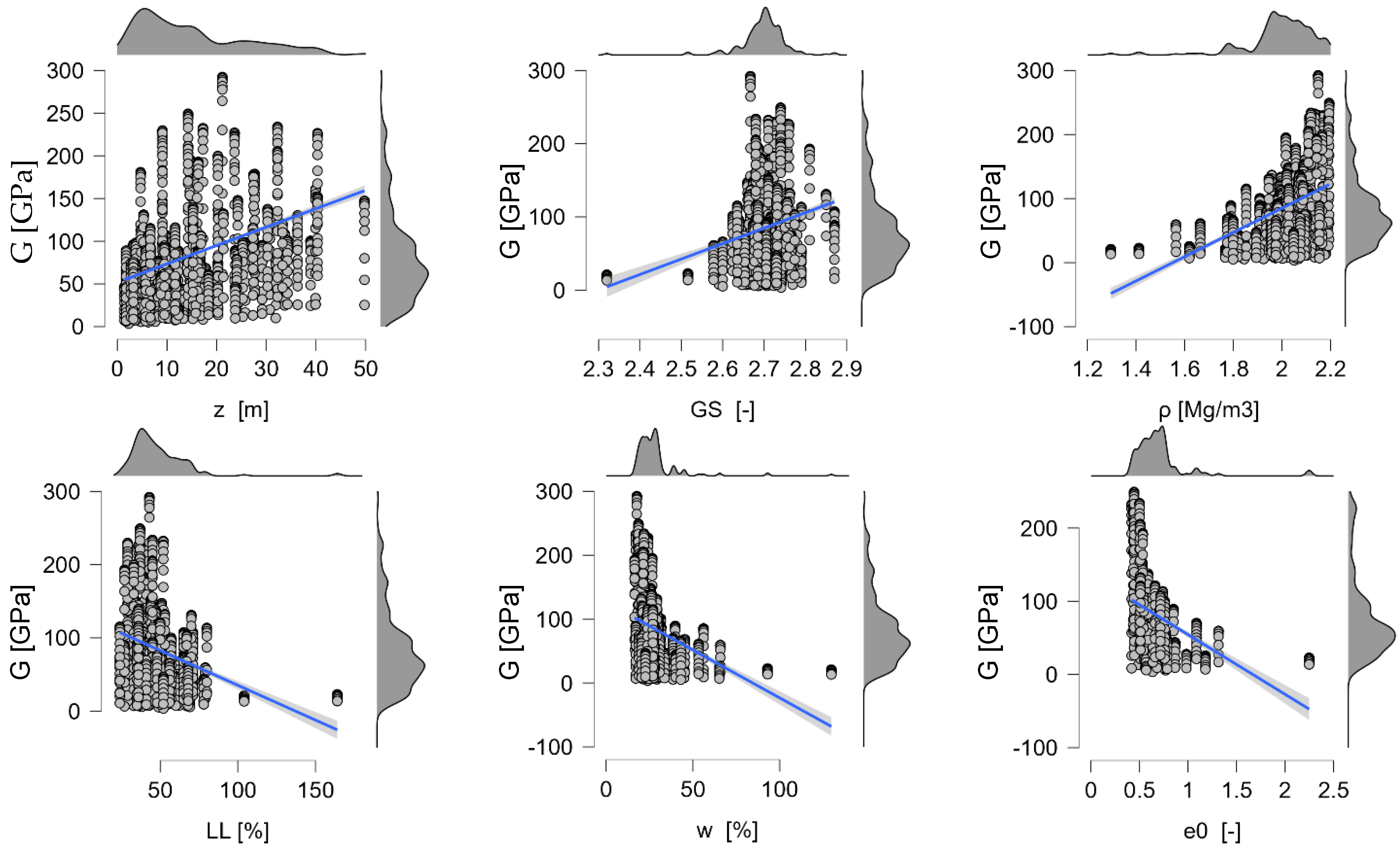
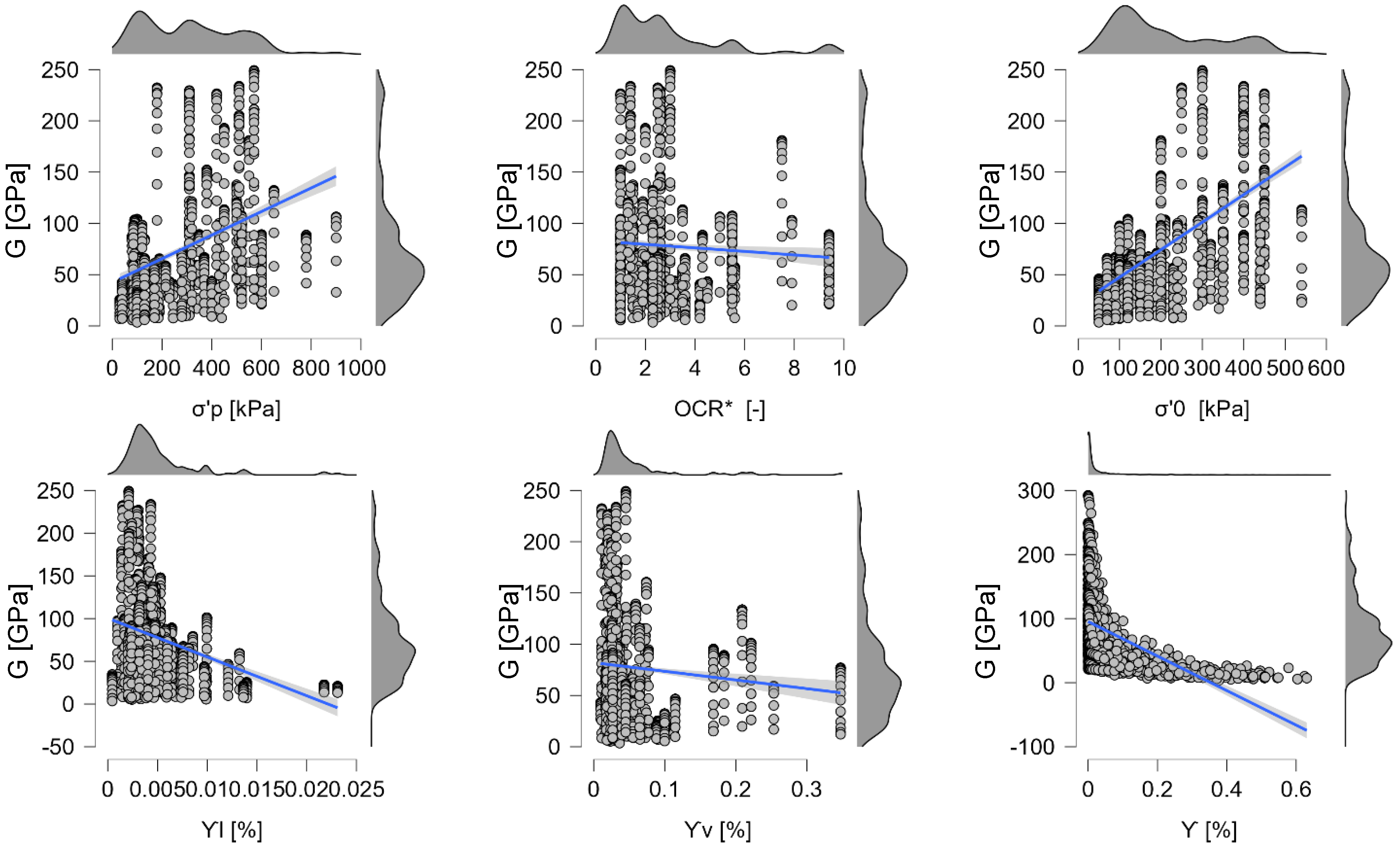
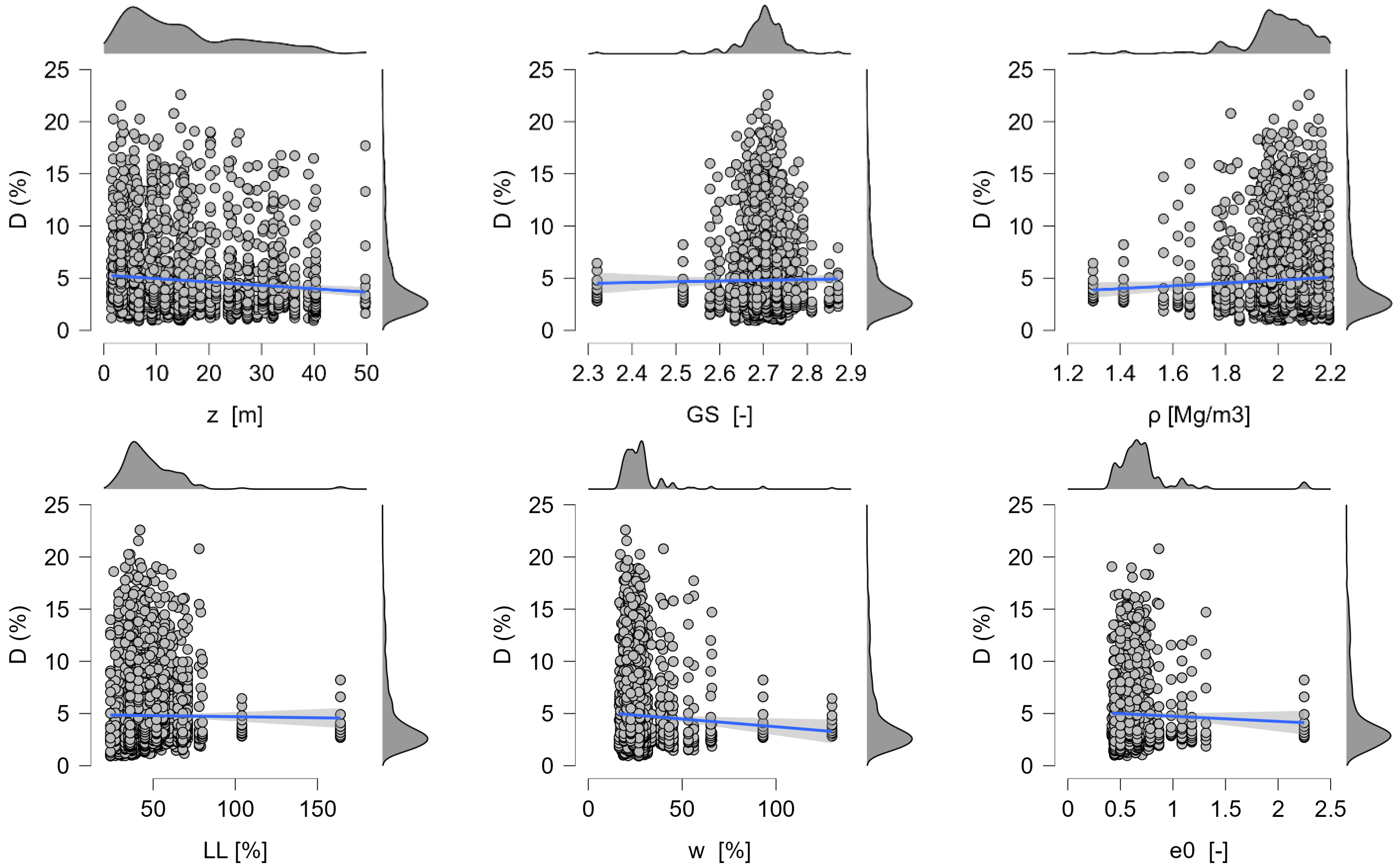
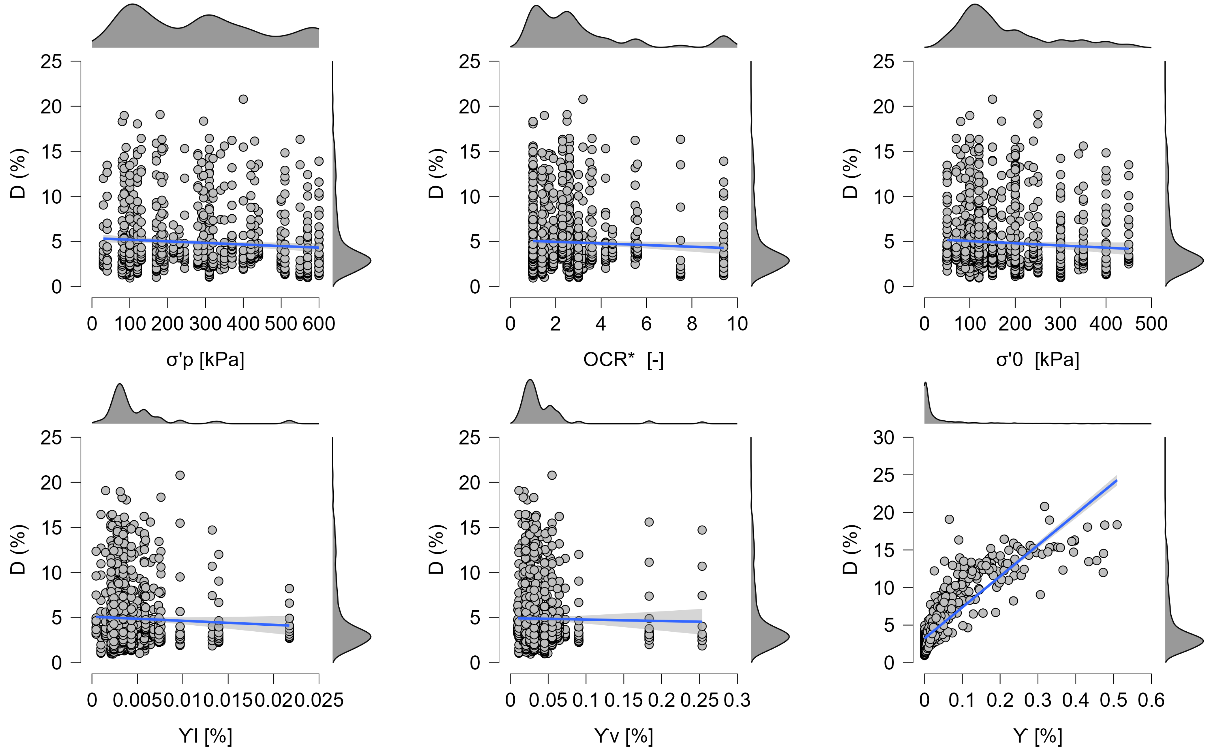
As shown in Table 2, a descriptive statistical summary of the retrieved features from the database is presented. One of the key parameters, G (shear modulus), stands out as a significant indicator of material stiffness. The mean value of 84,220, along with a standard deviation of 54,793, underscores the variability in stiffness among the tested materials. This variance in shear modulus implies that some materials are notably stiffer than others, which is a critical consideration for structural design. A higher shear modulus suggests that a material is less likely to deform under shear stress, making it suitable for load-bearing purposes. Conversely, the parameter D (damping) reflects the material’s ability to dissipate energy during dynamic loading. The average value of 4.8028, coupled with a standard deviation of 3.8141, indicates varying levels of energy dissipation capacity. Materials with higher damping ratios can better absorb and release energy during dynamic events, which is important for applications where vibrations or seismic forces need to be managed. The substantial standard deviation signifies that some materials exhibit significantly higher damping than others. Additionally, Figure 2 and Figure 3 shows the scatter relationship between G, D and other parameters. Grey areas illustrate the distribution of data points while indicate that there are no easily discernible patterns between shear modulus and damping versus the other input design factors. This suggests that conventional modeling techniques, such as linear regression, may not be sufficient to accurately model and investigate such relationships. Consequently, machine learning modeling techniques, which do not require predefined functional forms, appear to be a promising alternative.

4. Machine Learning Models (MLMs)

A framework known as machine learning (ML) includes a variety of algorithms and approaches that enable computers to learn from experience in a manner similar to how people naturally learn. Notably, ML algorithms can directly extract useful insights from data without the need for established mathematical models. Within machine learning, supervised and unsupervised learning are the two main subcategories. To train a model for predicting future outcomes using supervised methods, input and output data are used. The model might be discrete for classification tasks or continuous for regression tasks. In contrast, unsupervised techniques use only the input data and employ clustering to find patterns and structures in the data. In this study, a supervised regression ML approach was thought to be crucial for solving the current issue. In order to train a model that can forecast continuous output values, labeled data must be used. The authors have decided to use six distinct supervised regression approaches out of the many that are available: regression decision trees, support vector machines (SVMs), ensembles, Gaussian process regression (GPR), artificial neural networks (ANNs), and kernel methods. A brief description of each of these six ML algorithms will be provided in the paragraphs that follow.

4.1. Regression Decision Trees

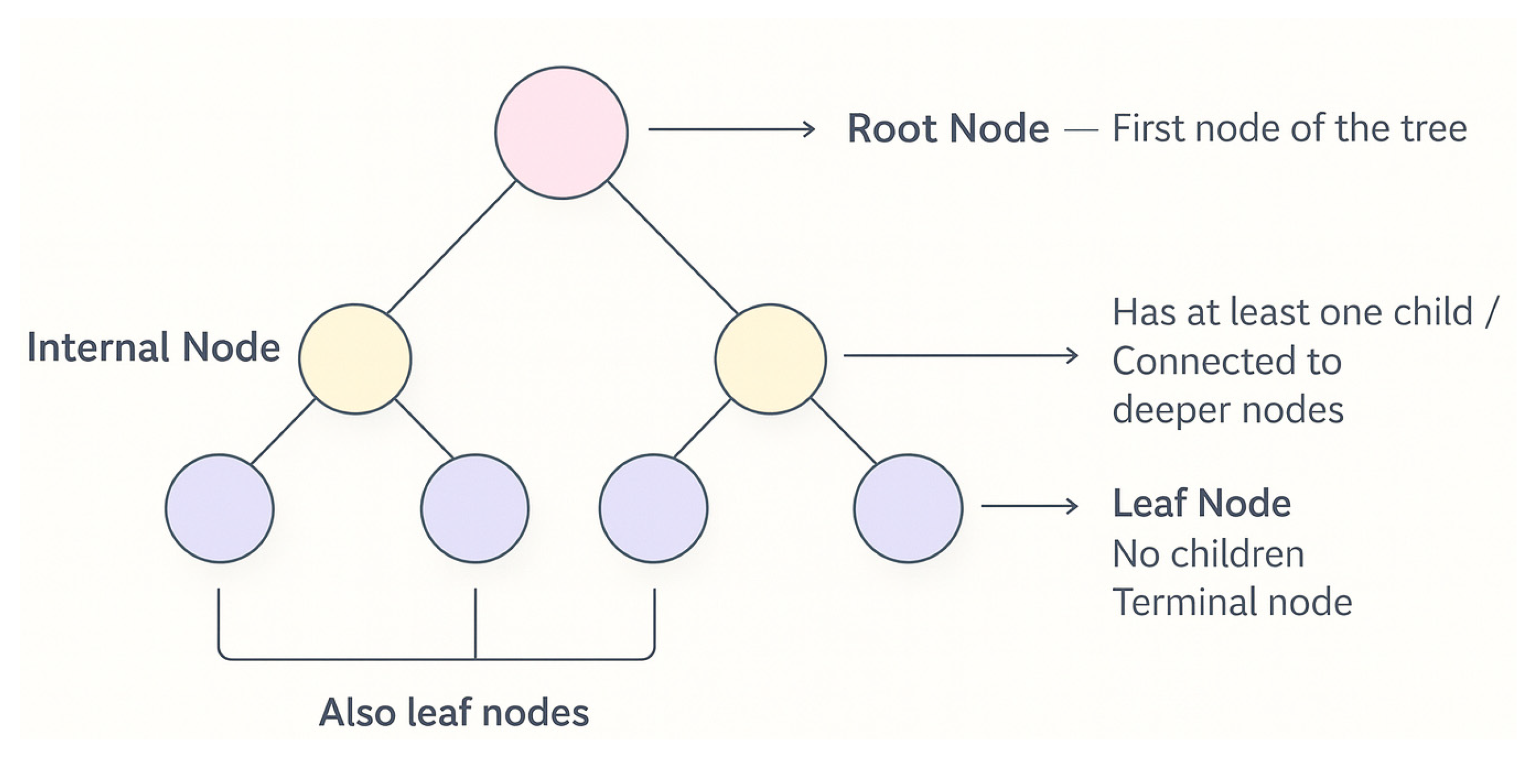
As seen in Figure 4, these regression trees, which resemble hierarchical structures with roots, branches, and leaves, are crucial for predicting numerical target variables [26,27].
In this application, the root node (the highest point in the tree) is where the regression decision tree algorithm starts the prediction process. The function performs conditional checks as it moves down the tree, passing through internal nodes, to choose the best branching path. This method is guided by a number of evaluation criteria, including the total sum of squared errors. The value assigned to the leaf node at the end of the calculated path ultimately determines the algorithm’s prediction result [36].
To divide and analyze data in a way that minimizes the deviation from the mean of the output characteristics is the key notion behind the methodology used in this study. This division is made possible by a sequence of splits, which essentially divide the data into various subgroups and allow the algorithm to spot underlying patterns and connections. Regression decision trees’ adaptability allows them to capture subtle variations in the data. As a result, they can be a powerful tool for predicting regression, especially when linear or nonlinear correlations between variables are difficult to detect. Regression decision trees are an important part of the process since they can help us find insights and improve the accuracy of the regression forecasts.
Regression tree construction is governed by the overall goal of minimizing the total deviation (DTotal) of the output features from the mean [37]. The equation serves as a representation of this idea.
D Total   = Y i Y 2
In this case, Yi stands in for the target feature and Y for the mean of the output features. The decrease in DTotal can be stated as follows since a segmentation point divides the data into two unique and nonoverlapping groups (left and right):
Δ j   Total   = D Total   D Right   + D Left  
Here, DRight and DLeft are the differences in deviation from subsets of the right and left, respectively.

4.2. Support Vector Machine

The support vector machine (SVM) method is usually utilized for efficient regression prediction. SVM is a sophisticated machine learning technique used to estimate numerical target outcomes and model complex relationships between variables. SVM is fundamentally based on the idea of structural risk minimization, which makes it possible to generalize effectively even with limited training data. The core idea of SVM entails generating a linear regression function in a higher-dimensional feature space where input data are transformed by nonlinear functions. Finding complicated correlations that might be concealed in the original data is made easier by this approach [38].
In this study, SVM has been tailored for applications involving regression, where it builds a regression model to forecast future outcomes based on existing input data. SVM does this by solving a convex quadratic optimization problem to optimize a regression model that fits with the knowledge and data patterns already known. The capacity of SVM to adapt to small sample sizes, which ensures accurate predictions even in circumstances with few data points, is one of its significant strengths. There are several SVM variations available, including linear, quadratic, and cubic SVMs, each of which has a unique set of kernel functions that determines how well the method performs. The scope and difficulty of the problem influence the choice of the kernel function, allowing us to adapt the approach to the particular regression prediction challenge.
The mathematical kernel function (k) expressed by the equation K (x, y) = [1 + (x, y)]P plays a role in several SVM models. The parameter P serves as a crucial determinant for the SVM kernel type, distinguishing between linear, quadratic, or cubic variations. Additionally, SVM can be categorized into fine, medium, and coarse Gaussian classes, with the kernel scale differentiating them. Specifically, for these classes, the kernel scale values are as follows: P/4 for the fine class, P for the medium class, and P^4 for the coarse class, with P representing the number of predictors used in the model.
While the fundamental concepts of the current SVM approach were initially proposed by Cortes and Vapnik in 1995 [39], SVMs have since gained widespread recognition and are now embraced by an expanding community of researchers [29,40].

4.3. Ensembles

In research, ensemble methods, which are well known for their capacity to combine information from various individual models, offer a practical means of increasing forecast accuracy. Particularly, ensemble trees, such as bagged trees and boosted trees, are promising in the current regression prediction procedure. These techniques make use of the combined knowledge of many decision trees, each of which adds a unique viewpoint to the overall predicted model [41,42].
Bootstrap aggregating, also known as bagging trees, is the process of building numerous decision trees using different bootstrapping samples of the dataset. Each tree makes a contribution to the final prediction, and the diversity of those predictions is cleverly used to produce a more reliable and accurate result. Bagged trees have the innate capacity to minimize overfitting by reducing the impact of outliers and noise in the data. Boosted trees, on the other hand, use an iterative process to improve the efficiency of each constituent tree. Instances that were incorrectly classified in earlier iterations are given more weight during boosting, instructing succeeding trees to concentrate on these difficult cases. This iterative learning procedure makes it possible to build a strong ensemble that continuously improves its predictions, leading to a regression model that is increasingly precise and well tuned [30,43].
Ensemble trees take advantage of the positive aspects of the individual components while minimizing the negative aspects. By combining the predictions of various trees, the ensemble can detect complex correlations in the dataset that individual models might miss. As a result, the ensemble tree technique improves the ability to generalize the developed regression models for prediction outside of the training set of data. The mathematical representation of an ensemble regression tree is expressed as follows:
y ˆ b a g ( x ) = 1 B b = 1 B   Y ˆ b ( x )
where y ˆ b a g ( x ) represents the target value obtained through averaging, Y ˆ b ( x ) signifies the predicted target value for observation x in the b-th bootstrap sample, and B denotes the total number of bootstrap samples.

4.4. Gaussian Process Regression

The effectiveness and adaptability of Gaussian process regression (GPR) have great potential in modeling the nonlinear behavior of dynamic properties. It utilizes the ideas of uncertainty quantification and nonparametric modeling. The foundation of GPR is the idea of using the adaptability of Gaussian processes to infer hidden correlations in data. GPR employs a more flexible strategy by learning directly from the data, in contrast to conventional regression algorithms that impose preset functional shapes. GPR’s versatility enables it to capture intricate and irregular patterns that could be difficult for parametric approaches to understand. GPR’s outstanding capacity to measure uncertainty is one of its most impressive features [44,45]. In this study, GPR offers estimates of associated uncertainty in addition to predictions. This information is extremely helpful, especially when dealing with real-world situations that are unpredictable by nature and have measurement noise. GPR instills a measure of confidence in its forecasts, improving the dependability of the regression models [46].
A Gaussian process is used in GPR to model the relationship between the input variables and the corresponding output values. A mean function and a covariance function, which express central tendency and spatial correlation, respectively, describe this process. Through Bayesian inference, GPR continuously improves its grasp of the underlying relationships and adjusts its predictions in accordance with the information at hand [47]. GPR also provides versatility thanks to its wide variety of kernel functions. GPR can be customized to fit the specifics of the collected dataset by choosing the right kernel function. According to smoothness, periodicity, or spatial correlation, each kernel represents a certain kind of link. This adaptability enables GPR to identify a wide range of complex patterns in the data.
Using a Gaussian distribution to simulate random variables, GPR modeling adopts a stochastic methodology. Squared exponential GPR, Matern GPR, exponential GPR, and rational quadratic GPR are all components of the Gaussian process. The choice of kernel function used in each scenario is what distinguishes these requirements, as seen below:
  • Squared Exponential Kernel:
K S E x , x = σ 2 exp ( x x ) 2 2 l 2
Here, l = characteristic length scale, and σ = constant value.
  • Matern Kernel:
K m = 1 2 v 1 T ( v ) 2 v l r v k v 2 v l r
Here, υ value depends on the input distance, and kυ denotes a modified Bessel function. The variables r and T are explained as follows:
T = l 2 r = x x
  • Exponential Kernel:
K E = e x p r l γ
Here, 0 < γ ≤ 2.
  • Rational Quadratic Kernel:
    K R Q = ( x , x ) = 1 + ( x x ) 2 2 α l 2 α
    where α depends on the input distance.

4.5. Artificial Neural Networks (ANNs)

Artificial neural networks (ANNs) provide a data-driven, universal-approximation approach that is well suited to capturing the nonlinear dependencies of G and D on stress, strain, and index properties. In this study, we used feed-forward multilayer perceptrons trained with supervised regression objectives (mean squared error) under 10-fold cross-validation. A typical network maps the standardized input vector x R p to the prediction y ^ via stacked affine transformations and nonlinear activations,
y ^ = W L ϕ ( ϕ ( W 2 ϕ ( W 1 x + b 1 ) + b 2 ) ) + b L ,
where W l ,   b l are layer weights and biases, and ϕ ( ) is a smooth nonlinearity (ReLU or tanh in our presets). To probe capacity–generalization trade-offs, we considered five presets consistent with MATLAB’s regression learners: narrow, medium, and wide single-hidden-layer networks (increasing neuron counts), and bilayered and trilayered deeper networks (two and three hidden layers, respectively). Training used scaled inputs, Glorot initialization, mini-batch gradient descent with adaptive learning rate, and l 2 weight decay; early stopping on a cross-validation fold prevented overfitting.
From a practical standpoint, ANNs can match top accuracy on G when sufficient data are available (Table 3), but they introduce additional hyperparameters (width, depth, learning rate, and regularization) and longer training times than single trees or bagged ensembles. Prior geotechnical applications of neural networks to cyclic/dynamic behavior further motivate their inclusion here [22,25,48].

4.6. Kernel Methods (Regularized Kernel Regression)

Kernel methods perform nonlinear regression by mapping inputs to a high-dimensional feature space where a linear estimator is learned implicitly through a positive-definite kernel k ( x , x ) . We adopt the regularized least-squares (kernel ridge) formulation, which yields the closed-form predictor:
f ^ ( x ) = k ( x ) ( K + λ I ) 1 y ,
where K i j = k ( x i , x j ) is the n × n Gram matrix over the training set, λ > 0 controls smoothness (penalizing model complexity), and k ( x ) = [ k ( x , x 1 ) , , k ( x , x n ) ] . This approach can approximate complex relationships while keeping a convex objective and a few hyperparameters.
Consistent with our SVM and GPR kernels, we evaluated standard choices for k : linear (baseline), polynomial (degree p ), and Gaussian/RBF with bandwidth (kernel scale) selected by cross-validation. We also tested MATLAB’s least-squares regression kernel preset used in Table 3 and Table 4. Inputs were standardized, λ and kernel scale were tuned within the 10-fold CV loop, and numerical stability was ensured by adding a small jitter to K when needed. Operationally, kernel regression is attractive for medium-sized datasets because it avoids iterative training of deep architectures and can capture smooth nonlinear effects of σ 0 , e 0 , ρ , γ , and plasticity indices. However, its O ( n 3 ) solve and sensitivity to kernel scale can limit scalability and robustness.

5. Results and Discussion

5.1. Feature Importance

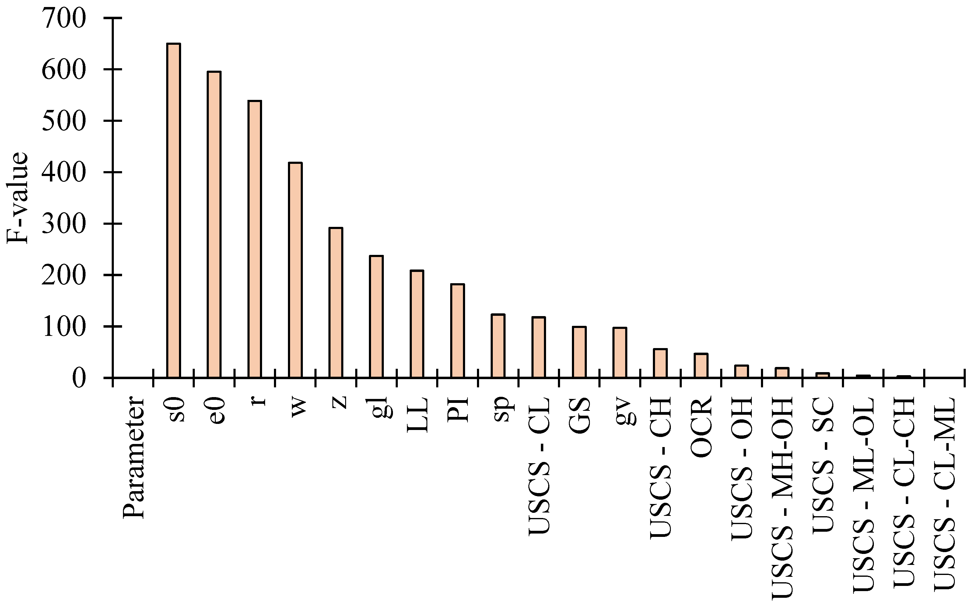
An F-test was conducted to assess the variability of different parameters, with the goal of identifying those that significantly influence shear modulus. Among the examined parameters, several stood out with notably high F-test values, indicating their strong influence on shear modulus.
According to Figure 5, test confining pressure (S0) demonstrated the highest F-test value of 649.8384, making it the most influential parameter for shear modulus. Following closely, the initial void ratio (e0) exhibited a substantial F-test value of 595.3, further emphasizing its significance in contributing to variation. Soil density also displayed a considerable F-test value of 538.8059, placing it among the top influential factors.
Additionally, parameters such as water content, depth of sample, elastic threshold, and liquid limit displayed substantial F-test results, suggesting their noteworthy contributions to the shear modulus variability. The F-test values for these parameters are 417.9, 291.8, 237.2, and 208.6, respectively.
On the other hand, while “USCS-CL” and specific gravity showed F-test values of 117.91 and 99.12, indicating moderate influence, the parameters such as volumetric threshold, “USCS-CH”, overconsolidation ratio, “USCS-OH”, “USCS-MH-OH”, “USCS-SC”, “USCS-ML-OL”, and “USCS-CL-CH” had relatively lower F-test values, suggesting less impact on shear modulus.
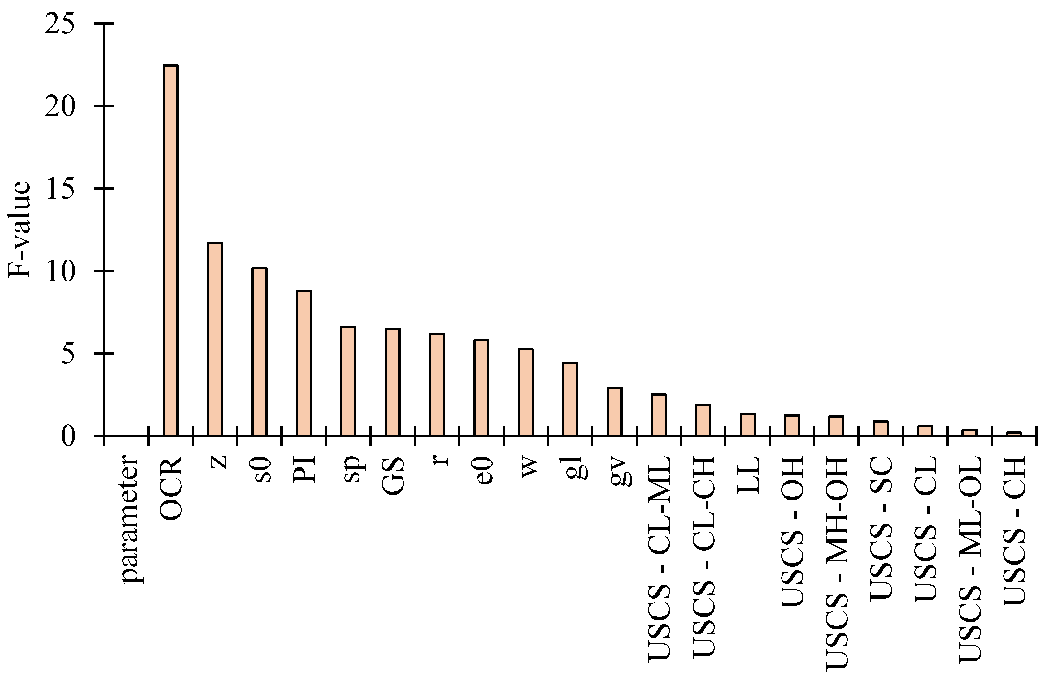
Figure 6 presents the results of an F-test analysis aimed at clarifying how different parameters influence the variability of damping, a crucial parameter in geotechnical engineering that gauges a material’s capacity to dissipate energy during deformation. The F-test values presented here reveal the relative importance of each parameter in elucidating the observed variations in damping behavior.
With an F-test value of 22.45, the overconsolidation ratio (OCR) emerges as the most influential parameter. Higher OCR values significantly affect damping characteristics, signifying the importance of this factor in damping variability. Depth of sample follows closely with an F-test value of 11.7, indicating its substantial influence on damping behavior. Variations in depth of sample can lead to notable changes in the damping properties. Test confining pressure ranks third in influence, with an F-test value of 10.2. It plays a vital role in shaping damping variability, and understanding its impact is crucial. Plasticity Index (PI): PI exhibits notable influence with an F-test value of 8.79. Higher PI values correlate with changes in damping behavior. Preconsolidation pressure demonstrates noticeable influence with an F-test value of 6.59. On the other hand, several parameters exert moderate influence, including specific gravity with a F-test value of 6.5, soil density with 6.20, initial void ratio with 5.8, water content with 5.25, volumetric threshold with 4.41, and elastic threshold with 2.93.

5.2. Shear Modulus Prediction Models

A comprehensive analysis was conducted in this section, which combines various machine learning techniques with traditional modeling approaches to predict shear modulus and damping. The models’ performances were evaluated using selected performance measures. The study of shear modulus prediction involves the utilization of diverse machine learning models, and a detailed analysis of these selected models was provided, considering key metrics such as RMSE, MSE, R2, MAE, and training time.
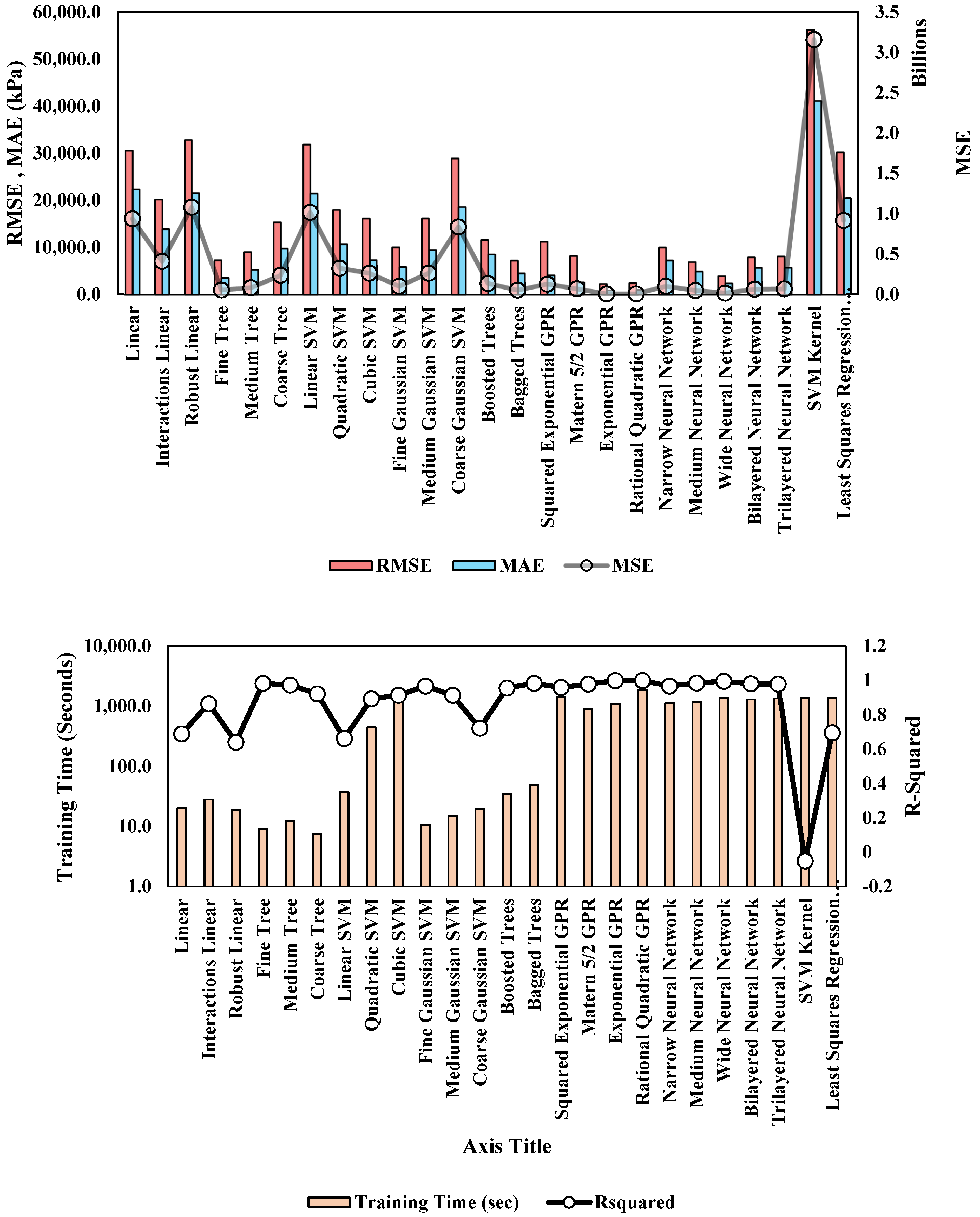
To mitigate the risk of over-fitting, a 10-fold cross-validation technique was employed for each model within both scenarios. Table 3 and Figure 7 show a visual comparison between the different specifications of each modeling technique for all-features. The following facts can be concluded:

5.2.1. Models’ Performance for Predicting Shear Modulus

The results demonstrate a wide range of performance among the models. Notably, the exponential GPR and rational quadratic GPR models stand out with exceptionally high R-squared values of 0.9983 and 0.9980, respectively. These models exhibit almost perfect fits to the data, highlighting their potential for precise shear modulus predictions.
Conversely, the SVM kernel model presents a unique challenge with a negative R-squared value of −0.0522. This unexpected result suggests a fundamental issue with its fit to the data, raising concerns about its applicability to the shear modulus prediction task.
The decision tree-based models, including fine tree, medium tree, and coarse tree, strike a balance between predictive accuracy and computational efficiency. With R-squared values ranging from 0.9214 to 0.9827, these models offer credible performance while requiring relatively shorter training times.
The neural network models, particularly the medium neural network and wide neural network, showcase strong predictive capabilities, with R-squared values ranging from 0.9667 to 0.9948. These models are appealing choices when precision is of utmost importance, even though they entail longer training times.

5.2.2. Partial Dependencies for Shear Modulus Models

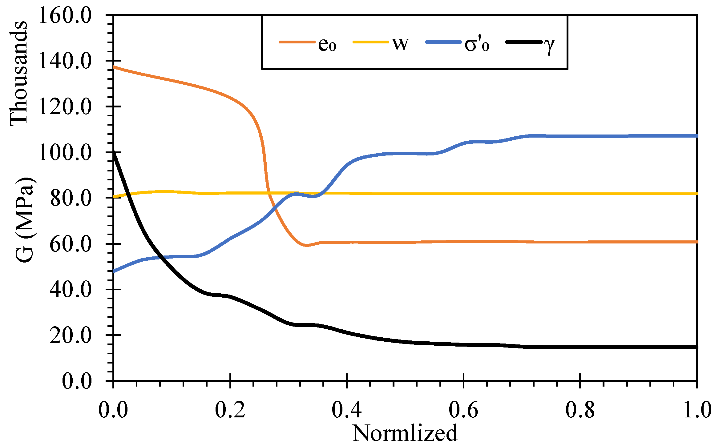
Figure 8 presents one-dimensional partial dependence (PD) curves for the four most influential predictors: initial void ratio e 0 , water content w , effective confining pressure s 0 (= σ 0 ), and shear-strain amplitude γ , computed from the operational bagged-tree model (10-fold CV). Predictors are normalized to [ 0 ,   1 ] ; each curve shows the marginal effect on G (MPa) after averaging over the empirical distribution of the remaining variables. Key trends align with soil mechanics:
  • G increases monotonically with s 0 and tends to plateau at higher normalized values, indicating diminishing stiffness gains once confinement is sufficiently high. This reflects stress-stiffening of the soil skeleton.
  • G decreases with e 0 . A sharper drop occurs across intermediate normalized values, consistent with the transition from denser to looser fabrics and loss of interparticle contact density.
  • G decays steeply at small strains, then approaches an asymptote, capturing the familiar stiffness-reduction behavior with increasing cyclic strain.
  • Within the sampled range, the marginal effect of w is weak to slightly negative after accounting for e 0 and plasticity indices, suggesting that the moisture state chiefly acts through correlated descriptors or interactions.

5.2.3. Computational Efficiency for Predicting Shear Modulus Models

Training times are a crucial consideration, especially in real-time or resource-constrained applications. Fine tree and coarse tree emerge as the quickest models to train, with training times of 8.94 s and 7.51 s, respectively. These models offer efficient solutions without sacrificing predictive accuracy.
On the other hand, Gaussian process regression (GPR) models, such as exponential GPR and rational quadratic GPR, demand more substantial computational resources, with training times of 1089.99 s and 1848.80 s, respectively. These models, while promising high accuracy, may be less practical in applications requiring real-time responsiveness.
Models like quadratic SVM and cubic SVM provide a trade-off between speed and accuracy, with training times of 443.44 s and 1238.73 s, respectively. They deliver credible predictive performance without the extended training times of GPR models.
In summary, the exponential GPR and rational quadratic GPR presets excel in predictive accuracy, while the fine tree model shines as the best option when considering both accuracy and training time.

5.3. Damping Prediction Models

5.3.1. Models’ Performance for Predicting Damping

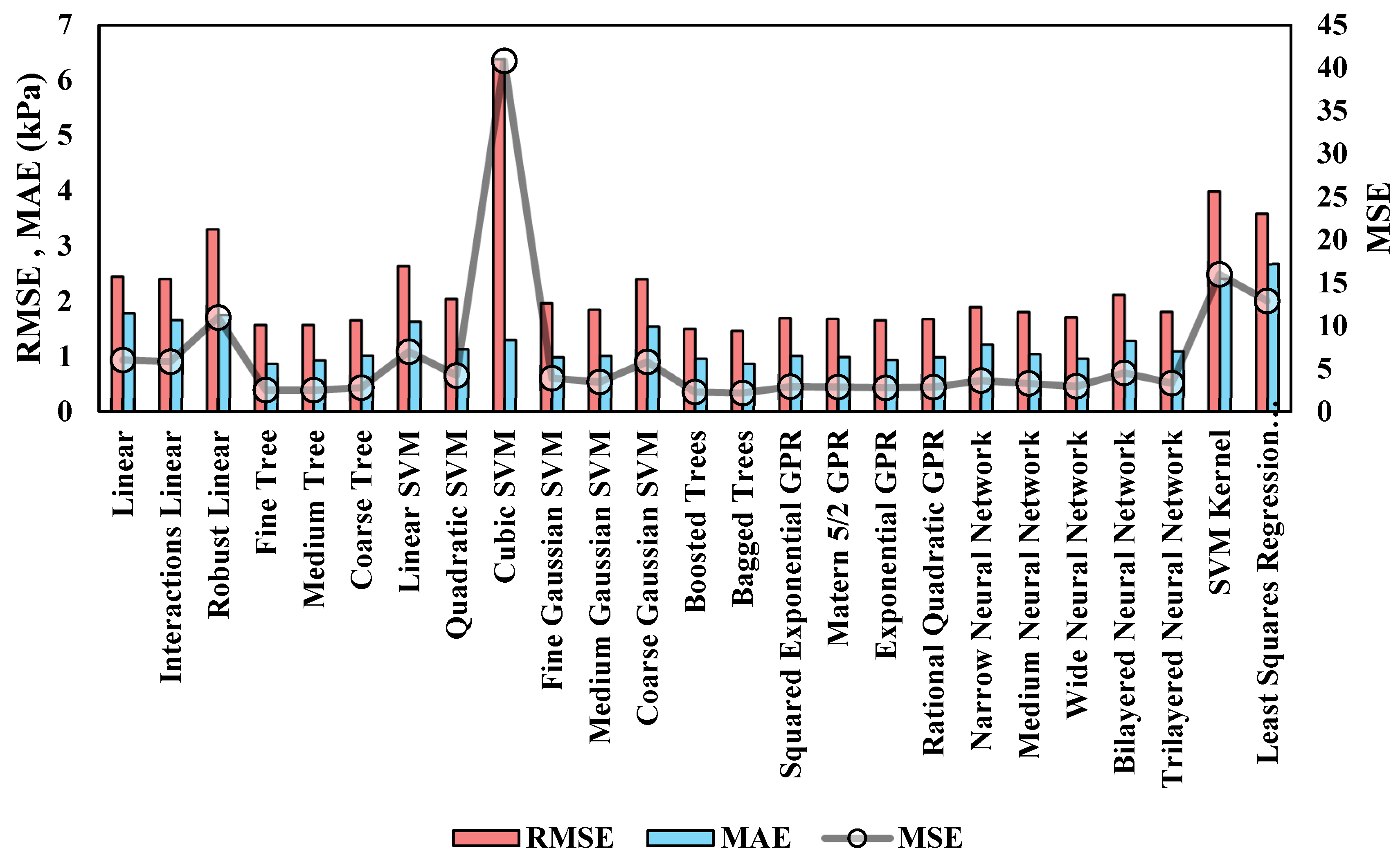
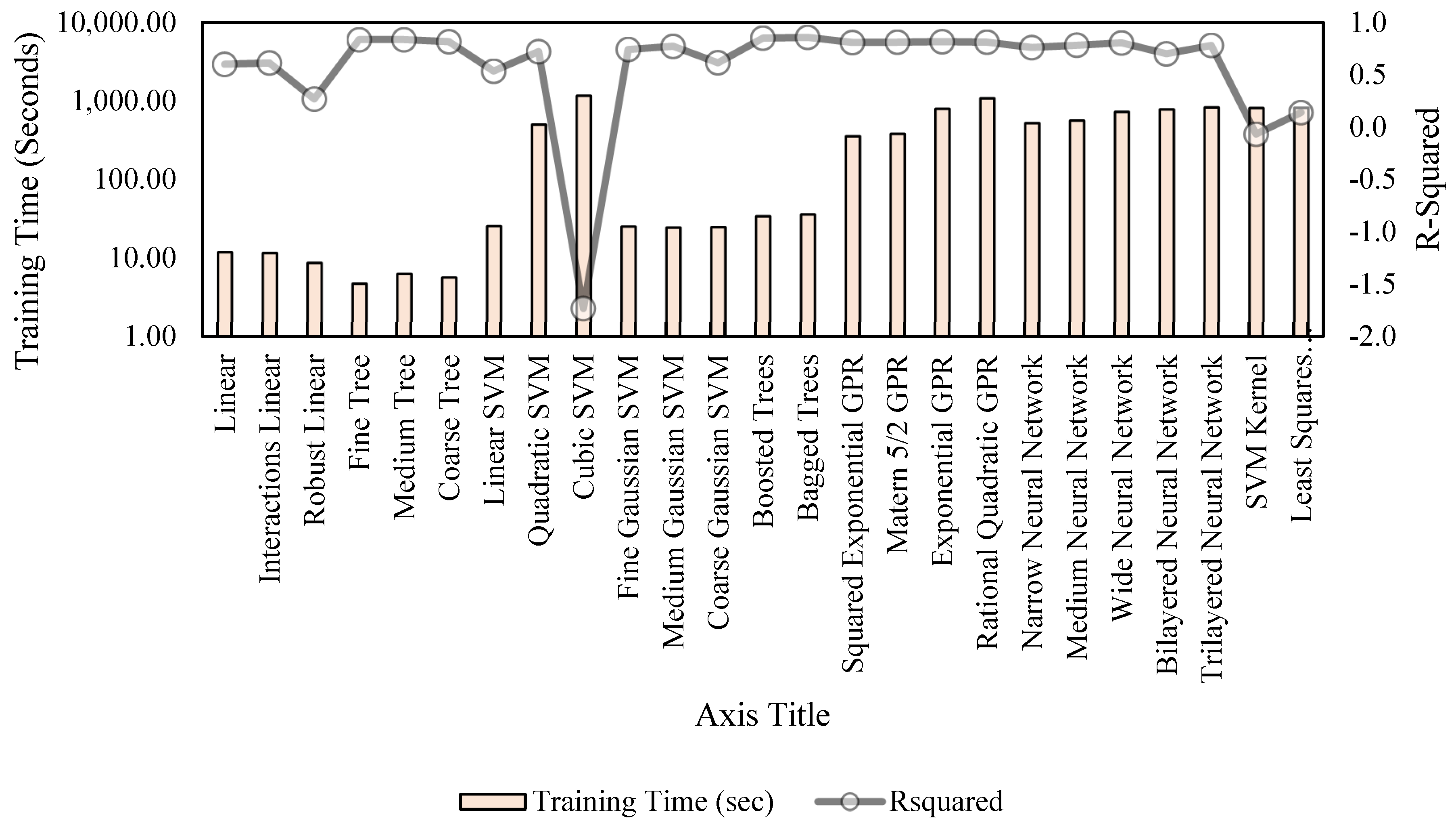
Table 4 and Figure 9 illustrate the results reveal a diverse spectrum of model performance. Notably, the bagged trees model shines as it boasts an impressive R-squared value of 0.8565, indicating a strong fit to the data. This model offers both accuracy and efficiency, with an RMSE of 1.4641 and an MAE of 0.8700. It demonstrates its potential as a practical choice for damping ratio prediction.
On the opposite end of the spectrum, the Cubic SVM model presents significant challenges with a negative R-squared value of −1.7334, indicating a poor fit to the data. This result raises concerns about the suitability of this model for accurate damping ratio predictions. Decision tree-based models, including fine tree, medium tree, and coarse tree, consistently offer a balanced performance, with R-squared values above 0.8. The fine tree model, in particular, stands out with an impressive R-squared of 0.8344. These models provide credible predictions without demanding extensive computational resources.

5.3.2. Partial Dependencies for Damping Models

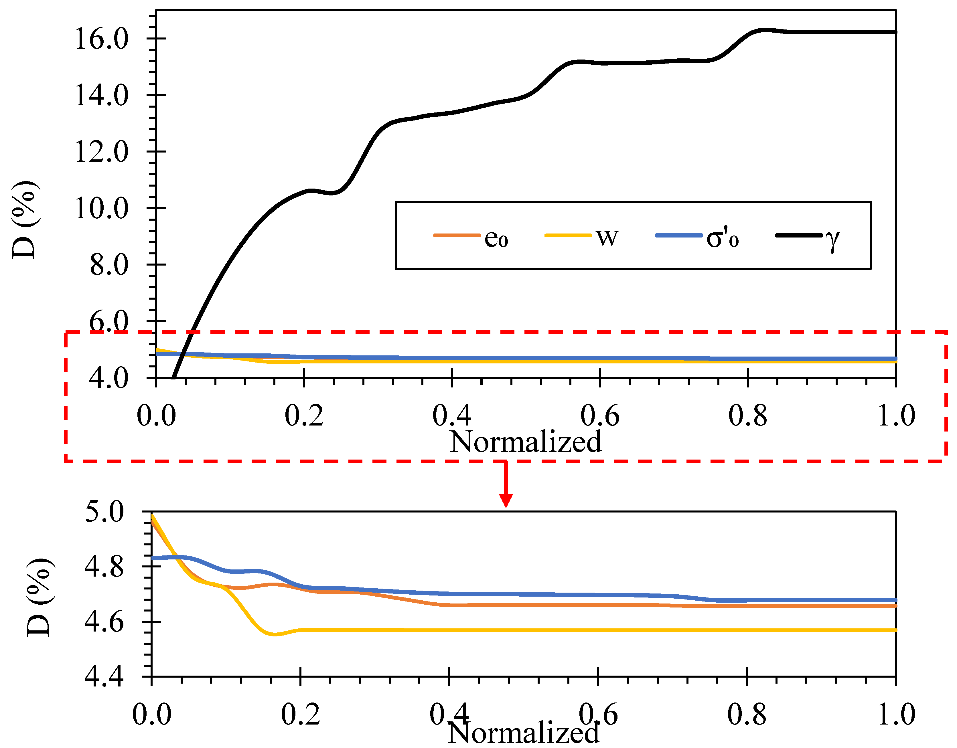
Figure 10 shows PD curves for D versus the same predictors ( e 0 , w , σ 0 , and γ ) from the bagged-tree model. The upper panel covers the full range; the lower panel magnifies the narrow band where the non- γ effects lie. Dominant and secondary behaviors are clear:
  • D increases strongly and monotonically with γ , approaching a gentle saturation at higher normalized strains. This reflects widening hysteresis loops and greater energy dissipation under larger cyclic strains.
  • A mild negative slope in s 0 suggests slightly lower D under higher confinement; consistent with tighter contacts and reduced micro-slip.
  • e 0 and w both exhibit small, smooth variations (sub-percent changes) over the observed range, indicating secondary roles once γ and s 0 are controlled. These effects may be partially mediated by plasticity and liquidity index, which interact with the moisture state.
Practically, the plots confirm that γ is the primary driver of D in this dataset, while s 0 exerts a modest moderating effect. The inset underscores that e 0 and w contribute only fine-scale adjustments useful for sensitivity checks but rarely decisive without concurrent changes in γ or plasticity.

5.3.3. Computational Efficiency for Damping Models

Training times play a crucial role in practical applications, particularly in real-time settings or those with resource constraints. Fine tree is the fastest model to train, taking just 4.7545 s. This combination of speed and accuracy makes it a compelling choice for scenarios where quick results are imperative. In contrast, Gaussian process regression (GPR) models like exponential GPR and rational quadratic GPR are time-consuming, with training times exceeding 800 s. While these models offer impressive accuracy, their computational demands may limit their applicability in time-sensitive situations. The quadratic SVM model stands out as a good compromise between accuracy and training time, with an R-squared of 0.7206 and a training time of 504.4546 s. This balance makes it a strong candidate for many practical applications.

5.4. Practical Implications and Recommendations

For engineering practice, model choice should balance accuracy, robustness, interpretability, and turnaround time. On that basis, bagged tree ensembles are recommended as the default operational model for both targets. They consistently achieve high accuracy for shear modulus (G) while training quickly and handling noisy, mixed-type inputs with minimal tuning. For damping ratio (D), bagged trees also perform strongly and are efficient enough for routine screening and parametric studies. When decisions are highly sensitive to the predicted value, particularly for D, where data scatter is typically larger, Gaussian process regression (GPR) with a rational-quadratic (or exponential) kernel is a valuable companion model because it delivers competitive point accuracy and, importantly, prediction intervals that can be carried into safety-factor and reliability checks. In time-critical settings or when interpretability is paramount (e.g., stakeholder reviews, quick field assessments), a fine or medium single decision tree provides transparent rules at modest accuracy loss and can serve as a diagnostic to sanity-check more complex learners. Support-vector machines and generic kernel regressors were less reliable in this application and generally require more careful scaling and tuning; neural networks can match top accuracy for G but add complexity without a clear practical advantage for most datasets of this size.
The predictors that most influence G in practice are the effective confining pressure (σ′0), initial void ratio (e0), and bulk density (ρ), with secondary but meaningful roles for water content (w), depth (z), and indices of clay mineralogy and consistency such as liquid limit (LL) and the elastic threshold (γl). These variables capture well-known mechanics: higher confinement and density stiffen the soil skeleton, while larger void ratio and higher water content reduce small-strain stiffness. The effect of strain amplitude (γ) is pivotal; stiffness reduction accelerates as γ increases, particularly under lower σ′0. Practitioners should therefore ensure that σ′0, e0, ρ, w, LL/PI, z, and γ are measured or estimated with care and are within the data ranges summarized in Table 2 before applying the model.
For D, overconsolidation ratio (OCR) and stress history (σ′p) emerge as primary controls alongside z, σ′0, and plasticity index (PI). These variables govern the breadth of hysteresis loops and microstructural rearrangements under cyclic loading. Interactions are often more informative than individual variables considered in isolation. In particular, the combinations σ′0 × γ (strain-dependent damping/stiffness at a given confinement), OCR × σ′0 (history-conditioned response under current stress), and PI × w are influential; the latter can be summarized as the liquidity index (LI ≈ (w − PL)/PI, with PL = LL − PI) to reflect proximity to the plastic–liquid transition. Where feasible, computing LI and including it (or monitoring the PI–w coupling) improves physical credibility and predictive stability. Although USCS classes help encode gross material type, their standalone importance is typically lower than that of the continuous stress, strain, and index descriptors; they should complement rather than replace those descriptors.
Two practical safeguards help ensure reliable deployment. First, respect the domain of applicability by enforcing input checks against the observed ranges (e.g., σ′0 ≈ 50–540 kPa, σ′p ≈ 30–900 kPa, PI ≈ 4–84%, LL ≈ 24–164%, w ≈ 16–130%, e0 ≈ 0.40–2.46, γ ≈ 1.9×10⁻⁵–0.63%), and flag extrapolations for engineering review. Second, because G and D are strain-dependent, results are more stable if predictions are segmented by strain band (e.g., γ < 0.01%, 0.01–0.1%, ≥0.1%) or if γ is explicitly retained and its monotonic influence verified. In model maintenance, periodic calibration with a small set of local resonant-column tests can correct site-specific bias with minimal effort. For assurance, simple interpretability diagnostics (e.g., permutation importance or partial-dependence trends) should be reviewed to confirm expected monotonic relations (e.g., G increasing with σ′0 at small strains, D increasing with γ over the working range).
For most workflows, the preferred application is to deploy bagged trees as the primary predictor for both G and D because they offer the best accuracy–speed–robustness trade-off, and to supplement with GPR when uncertainty quantification is needed for design-level decisions or when data are sparse. Emphasis should be placed on collecting high-quality measurements of σ′0, e0, ρ, w, LL/PI (or LI), OCR/σ′p, z, and γ, and on recognizing the key interactions among these variables. Adopting these recommendations will yield predictions that are both practically useful and consistent with soil mechanics, thereby supporting safer and more economical dynamic-response designs.

Using the Models to Advance Engineering Knowledge and Design Standards

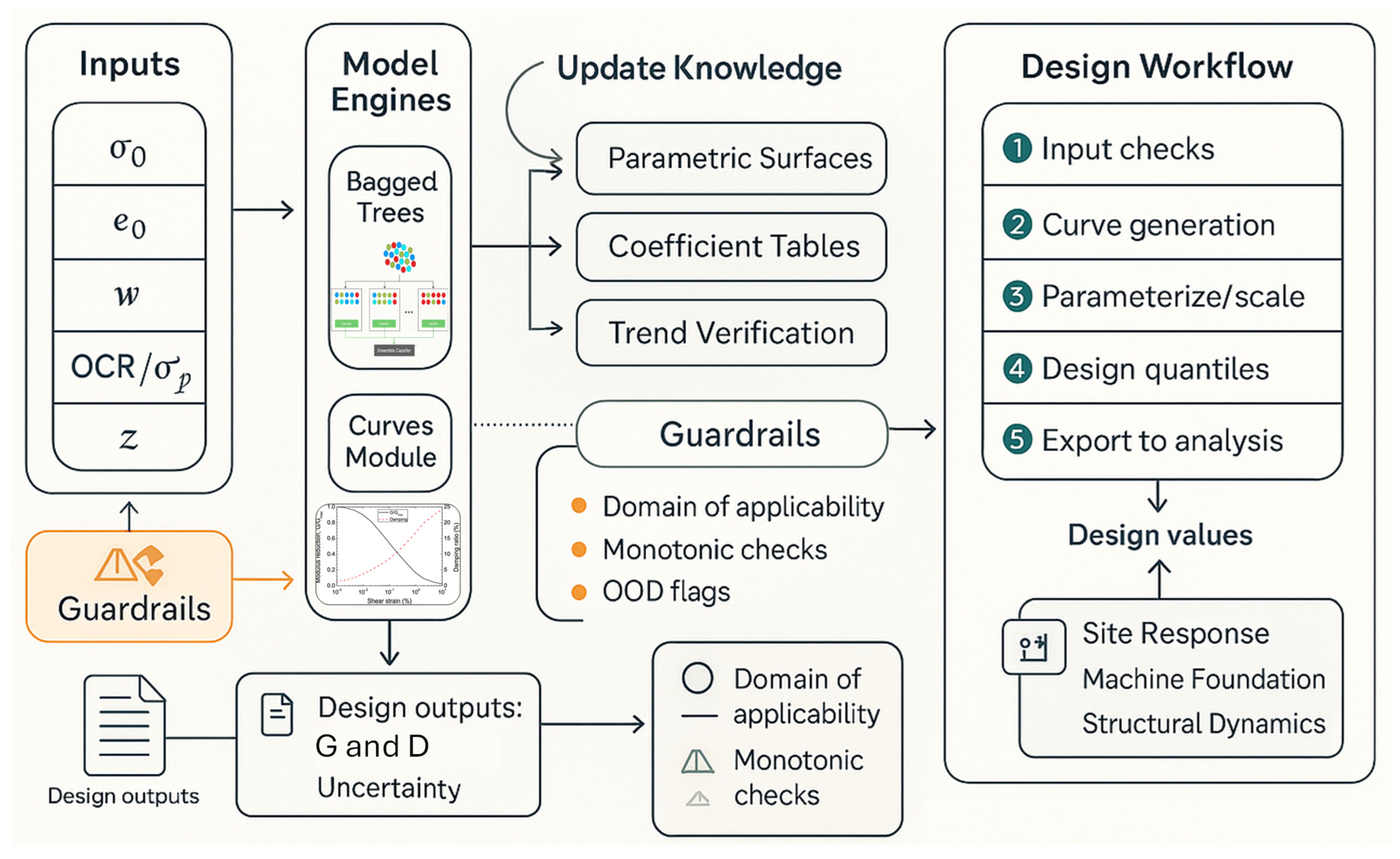
The bagged-tree predictor for G and the GPR companion for D convert routine descriptors: σ 0 , e 0 , ρ , w , L L / P I (or L I ), O C R / σ p , z , and γ into strain-compatible estimates with optional prediction intervals. This capability can (i) refine stiffness-reduction and damping-ratio knowledge with explicit dependence on stress, fabric, and moisture state; and (ii) provide code-ready inputs (or modifiers) that sit atop existing procedures rather than replacing them. An example of a framework-to-standards adoption is shown in Figure 11 and explained in detail as follows:
(A)
Updating modulus-reduction and damping knowledge
  • Mechanics-consistent trends, quantified through partial-dependence diagnostics, confirm expected monotonic relations: G with σ 0 , G with e 0 and γ ; D with γ , mild D with σ 0 . These trends can be published as parametric surfaces G ( γ , σ 0 , e 0 , ρ ) and D ( γ , σ 0 , O C R , P I ) , improving current charts that primarily index to plasticity or generic “soil type.”
  • From ML curves to compact parameters by code adoption and transparency, fit the ML-generated G ( γ ) and D ( γ ) grids to standard closed-form families (e.g., hyperbolic/sigmoidal for G / G m a x ; smooth saturating forms for D ). Publish coefficient tables as functions of σ 0 , L I (or w P I ), and O C R . This preserves code familiarity while embedding multivariate dependence learned from data.
(B)
Code-ready modifiers for existing standards
Let G chart ( γ ) and D chart γ be baseline curves from the current guidance. Multiplicative modifiers derived from the ML models are defined as follows:
α G ( σ 0 , e 0 , ρ , L I , ) = G ML ( γ 0 ) G chart ( γ 0 ) , β D ( σ 0 , O C R , P I , L I , ) = D ML ( γ \ * ) D chart ( γ \ * ) ,
which are evaluated at reference strains γ 0 (small-strain) and γ * (working-strain). α G and β D are applied across the full γ range (or with strain-band smoothing). This ML-informed scaling respects legacy workflows (equivalent-linear or nonlinear site response; machine foundation checks) while tailoring curves to site-specific stress history and index properties.
(C)
Uncertainty-aware design values
Where reliability or partial-factor formats are used, draw design values from quantiles of the GPR (for D ) or from conformalized ensembles (for G ):
  • Stiffness: G design ( γ ) = Q p   ( G ML ( γ ) ) with p chosen to align with code reliability targets;
  • Damping: D design ( γ ) = Q 1 p ( D ML ( γ ) ) .
    Report p , coverage diagnostics, and any conservatism factors so the selection is auditable.
(D)
A practical, code-compatible workflow
  • Verify all predictors lie within the trained domain (Table 2 ranges) and compute the liquidity index L I ( w P L ) / P I where available.
  • On a strain grid relevant to the analysis, compute G ( γ ) and D ( γ ) from the bagged-tree and GPR models; optionally segment by strain band ( < 0.01 % , 0.01 % 0.1 % and 0.1 % ).
  • Fit to the code’s chosen curve forms or compute α G , β D modifiers against baseline charts.
  • Choose p according to project criticality (e.g., standard vs. essential facilities) and extract quantile-based design values.
  • Provide tabulated G / G m a x ( γ ) and D ( γ ) pairs for site-response or machinery-vibration software, with a short model card (data ranges, CV metrics, and OOD flags).
  • If a few local RC or BE/Vs data exist, perform a light calibration step (bias correction or monotone-constrained refit) and re-export the curves.
(E)
Knowledge gaps made measurable
The models surface areas where present standards are weakest (e.g., combined effects of σ 0 × γ and P I × w ). By logging systematic deviations between ML-informed curves and code baselines, committees can prioritize targeted new testing (e.g., partially saturated states, frequency effects) and iterate the published parameter tables, thus turning the standard into a living, evidence-tracked artifact.

5.5. Limitations and Future Studies

The benchmark offers practical guidance, yet several constraints limit generalization and certainty. Addressing the following items would strengthen reliability, interpretability, and deployment value. Each limitation is paired with a targeted future direction.
  • Direct measures of soil fabric and microstructure, cementation/carbonate content, contact density/anisotropy, mineralogical fractions from X-ray diffraction (XRD), specific surface area and cation-exchange capacity (CEC), pore-size distribution and microcracks from scanning electron microscopy (SEM) and mercury intrusion porosimetry (MIP), and pore-fluid chemistry (salinity, pH) are absent and only indirectly proxied by LL/PI, water content, and USCS class. This omission likely explains part of the variance, especially in D , and can inflate the apparent role of covarying site variables (e.g., depth, σ 0 . Therefore, future studies should enrich datasets with these descriptors and quantify incremental value via ablation analysis and interpretable diagnostics (permutation importance, partial-dependence plots (PDPs), individual conditional expectation (ICE), and SHapley Additive exPlanations (SHAP)), verifying trends consistent with mechanics.
  • Degree of saturation, matric suction, loading frequency/strain-rate, and temperature are sparsely represented, restricting validity mainly to saturated, lab-controlled RC conditions within the tested bandwidths. Thus, future studies should incorporate partially saturated tests (reporting degree of saturation S r and suction), frequency/strain-rate sweeps, and temperature variation, and compare global models with strain-band models ( γ < 0.01 % , 0.01 0.1 % , 0.1 % ).
  • Alternative histories and anisotropic consolidations (e.g., varying K 0 ) are unevenly sampled; global fits can blur strain-dependent behavior. Therefore, future studies should expand stress-path coverage and encode it explicitly, or adopt multi-task/curve models to learn G ( γ ) and D ( γ ) with monotonicity checks ( G with σ 0 ; G with e 0 ; D with γ ).
  • Despite 2738 tests, some USCS classes are under-represented, and multiple specimens per site introduce correlation, making ordinary k-fold cross-validation optimistic for across-site transportability. Accordingly, future studies should apply grouped/site-wise, fully nested cross-validation with within-fold preprocessing, add site/campaign hold-outs, report dispersion across sites, and, where feasible, validate against independent field or small-strain lab measures (e.g., shear-wave velocity (Vs)-based G m a x , spectral analysis of surface waves (SASW), and bender-element (BE) tests).
  • Univariate F-tests are linear and do not capture interactions such as σ 0   ×   γ or P I   ×   w ; one-hot USCS encoding is coarse. Therefore, future studies should evaluate physics-motivated transforms and composites (e.g., log G ; normalization by mean effective stress p ; liquidity index L I ( w P L ) / P I , include interaction features, and address heteroscedasticity with variance-stabilizing targets.
  • Only Gaussian process regression yields native intervals; interval calibration and shift detection were not assessed systematically. Thus, future studies should implement quantile regression forests/boosting and conformal prediction to obtain calibrated coverage reporting prediction-interval coverage probability (PICP), mean prediction-interval width (MPIW), and continuous ranked probability score (CRPS) alongside simple range guards and out-of-distribution (OOD) detectors based on distance-to-training-manifold.
  • Tree-boosting variants common for tabular data (XGBoost, LightGBM, CatBoost) and probabilistic forests were not included; monotonic constraints aligned with mechanics were not enforced. Therefore, future studies should benchmark these families.

6. Conclusions

This study benchmarks widely used machine learning approaches for predicting two dynamic soil parameters, shear modulus (G) and damping ratio (D), from resonant-column data. Across 2738 tests and using uniform 10-fold cross-validation, linear models, decision trees, and ensembles, support-vector machines, Gaussian-process regression, and neural networks were evaluated using RMSE, MAE, MSE, and R2. The results indicate that algorithm choice materially affects performance and that no single method is uniformly superior across both targets.
For shear modulus, bagged tree ensembles delivered the most favorable accuracy–efficiency balance (R2 ≈ 0.98), offering high predictive fidelity with fast training and resilience to noisy, mixed-type inputs. For damping ratio, a rational-quadratic Gaussian-process model achieved the highest accuracy (R2 ≈ 0.81) and, uniquely, yields uncertainty estimates that can be propagated into design checks. These findings support a practical pairing: bagged trees as the operational model for routine predictions and Gaussian-process regression as a complementary tool when uncertainty quantification is required or when decisions are especially sensitive to D.
Feature-importance patterns align with geomechanics and provide guidance for data collection. Stiffness is governed primarily by effective confining pressure (σ′0), initial void ratio (e0), and density (ρ), with meaningful contributions from water content (w), depth (z), and plasticity measures. Damping behavior is driven by overconsolidation ratio (OCR) and stress history (σ′p) alongside σ′0, PI, and z. Interactions among these variables, particularly σ′0–γ (strain amplitude), OCR–σ′0, and PI–w (or liquidity index), are influential and should be represented explicitly or monitored to maintain physical credibility.
The models are most reliable within the observed input ranges and strain levels; extrapolation should be flagged for engineering review. Incorporating prediction intervals, segmenting by strain band, and performing light site-specific calibration when limited local tests are available can further increase reliability for design applications. Future extensions that embed physics-based constraints and monotonicity, expand datasets to additional soil groups and loading paths, and integrate field-scale measurements will enhance generalization and interpretability. Overall, the results demonstrate that carefully selected machine learning models can provide accurate, efficient, and defensible estimates of G and D, complementing conventional dynamic-soil analyses and supporting safer, more economical designs.

Author Contributions

Conceptualization, A.A., M.G.A., M.O. and E.A.; Methodology, A.A.; Software, A.A. and E.A.; Formal analysis, A.A. and M.G.A.; Investigation, M.G.A., M.O. and E.A.; Resources, M.O.; Data curation, M.O. and E.A.; Writing—original draft, A.A., M.G.A., M.O. and E.A.; Writing—review & editing, A.A., M.G.A., M.O. and E.A.; Visualization, A.A., M.G.A., M.O. and E.A.; Supervision, M.G.A., M.O. and E.A.; Project administration, M.G.A. and M.O. All authors have read and agreed to the published version of the manuscript.

Funding

This research received no external funding.

Data Availability Statement

The original contributions presented in the study are included in the article, further inquiries can be directed to the corresponding author.

Conflicts of Interest

The authors declare no conflict of interest.

References

  1. Terzaghi, K.; Peck, R.B.; Mesri, G. Soil Mechanics in Engineering Practice; John Wiley & Sons: Hoboken, NJ, USA, 1996. [Google Scholar]
  2. Seed, H.B.; Idriss, I.M. Soil moduli and damping factors for dynamic response analyses. Earthq. Eng. Struct. Dyn. 1970, 1, 7–26. [Google Scholar]
  3. ASTM D4015-15; Standard Test Method for Modulus and Damping of Soils by the Resonant-Column Method. ASTM International: West Conshohocken, PA, USA, 2015.
  4. Phoon, K.K.; Kulhawy, F.H. Characterization of geotechnical variability. Can. Geotech. J. 1999, 36, 612–624. [Google Scholar] [CrossRef]
  5. Kramer, S.L. Geotechnical Earthquake Engineering; Prentice Hall: Upper Saddle River, NJ, USA, 1996. [Google Scholar]
  6. Gazetas, G. Formulas and charts for impedances of surface and embedded foundations. J. Geotech. Eng. 1991, 117, 1363–1381. [Google Scholar] [CrossRef]
  7. Wolf, J.P. Foundation Vibration Analysis Using Simple Physical Models; Prentice Hall: Englewood Cliffs, NJ, USA, 1994. [Google Scholar]
  8. Demir, A.; Demir, S.; Sahin, E.K. Machine Learning Based Prediction of Peak Floor Acceleration in Low- to Mid-Rise RC Buildings Using Ground Motion Intensity Measures. Iran. J. Sci. Technol. Trans. Civ. Eng. 2025, 1–25. [Google Scholar] [CrossRef]
  9. Park, D.; Kishida, T. Shear modulus reduction and damping ratio curves for earth core materials of dams. Can. Geotech. J. 2019, 56, 14–22. [Google Scholar] [CrossRef]
  10. Vucetic, M.; Dobry, R. Effect of soil plasticity on cyclic response. J. Geotech. Eng. 1991, 117, 89–107. [Google Scholar] [CrossRef]
  11. Darendeli, M.B. Development of a New Family of Normalized Modulus Reduction and Material Damping Curves for Cohesive Soils. Ph.D. Dissertation, The University of Texas at Austin, Austin, TX, USA, 2001. [Google Scholar]
  12. Kazemi, F.; Jankowski, R. Machine learning-based prediction of seismic limit-state capacity of steel moment-resisting frames considering soil-structure interaction. Comput. Struct. 2022, 274, 106886. [Google Scholar] [CrossRef]
  13. Salgado, R.; Kim, D. Shear wave velocity and soil liquefaction. J. Geotech. Geoenviron. Eng. 2009, 135, 956–967. [Google Scholar]
  14. Kumar, S.S.; Krishna, A.M.; Dey, A. Parameters influencing dynamic soil properties: A review treatise. In Proceedings of the National Conference on Recent Advances in Civil Engineering, Kalavakkam, India, 15–16 November 2013; pp. 1–10. [Google Scholar]
  15. Kallioglou, P.; Tika, T.; Pitilakis, K. Shear modulus and damping ratio of cohesive soils. J. Earthq. Eng. 2008, 12, 879–913. [Google Scholar] [CrossRef]
  16. Lin, B.; Zhang, F.; Feng, D.; Tang, K.; Feng, X. Dynamic shear modulus and damping ratio of thawed saturated clay under long-term cyclic loading. Cold Reg. Sci. Technol. 2018, 145, 93–105. [Google Scholar] [CrossRef]
  17. Zhang, J.; Andrus, R.D.; Juang, C.H. Normalized shear modulus and material damping ratio relationships. J. Geotech. Geoenviron. Eng. 2005, 131, 453–464. [Google Scholar] [CrossRef]
  18. Kallioglou, P.; Tika, T.; Koninis, G.; Papadopoulos, S.; Pitilakis, K. Shear modulus and damping ratio of organic soils. Geotech. Geol. Eng. 2009, 27, 217–235. [Google Scholar] [CrossRef]
  19. Gaudiosi, I.; Romagnoli, G.; Albarello, D.; Fortunato, C.; Imprescia, P.; Stigliano, F.; Moscatelli, M. Shear modulus reduction and damping ratios curves joined with engineering geological units in Italy. Sci. Data 2023, 10, 625. [Google Scholar] [CrossRef]
  20. Dash, S.R.; Sharma, M.L. Applications of artificial intelligence in geotechnical engineering. In Handbook of Applications of Machine Learning; Springer: Berlin/Heidelberg, Germany, 2018; pp. 381–398. [Google Scholar]
  21. Pirnia, P.; Duhaime, F.; Manashti, J. Machine learning algorithms for applications in geotechnical engineering. In Proceedings of the GeoEdmonton, Edmonton, AB, Canada, 23–26 September 2018; pp. 1–37. [Google Scholar]
  22. Zhang, W.; Li, H.; Li, Y.; Liu, H.; Chen, Y.; Ding, X. Application of deep learning algorithms in geotechnical engineering: A short critical review. Artif. Intell. Rev. 2021, 54, 5633–5673. [Google Scholar] [CrossRef]
  23. Puri, N.; Prasad, H.D.; Jain, A. Prediction of geotechnical parameters using machine learning techniques. Procedia Comput. Sci. 2018, 125, 509–517. [Google Scholar] [CrossRef]
  24. Zhang, P.; Yin, Z.-Y.; Jin, Y.-F. Machine learning-based modelling of soil properties for geotechnical design: Review, tool development and comparison. Arch. Comput. Methods Eng. 2022, 29, 1229–1245. [Google Scholar] [CrossRef]
  25. Baghbani, A.; Choudhury, T.; Costa, S.; Reiner, J. Application of artificial intelligence in geotechnical engineering: A state-of-the-art review. Earth-Sci. Rev. 2022, 228, 103991. [Google Scholar] [CrossRef]
  26. Phoon, K.K.; Zhang, W. Future of machine learning in geotechnics. Georisk Assess. Manag. Risk Eng. Syst. Geohazards 2023, 17, 7–22. [Google Scholar] [CrossRef]
  27. Zhang, W.; Gu, X.; Tang, L.; Yin, Y.; Liu, D.; Zhang, Y. Application of machine learning, deep learning and optimization algorithms in geoengineering and geoscience: Comprehensive review and future challenge. Gondwana Res. 2022, 109, 1–17. [Google Scholar] [CrossRef]
  28. Zhong, X.G.; Zeng, X.; Rose, J.G. Shear modulus and damping ratio of rubber-modified asphalt mixes and unsaturated subgrade soils. J. Mater. Civ. Eng. 2002, 14, 496–502. [Google Scholar] [CrossRef]
  29. Ma, G.; Chao, Z.; Zhang, Y.; Zhu, Y.; Hu, H. The application of support vector machine in geotechnical engineering. In IOP Conference Series: Earth and Environmental Science; IOP Publishing: Bristol, UK, 2018; Volume 189, p. 022055. [Google Scholar]
  30. Loh, W.Y. Classification and regression trees. Wiley Interdiscip. Rev. Data Min. Knowl. Discov. 2011, 1, 14–23. [Google Scholar] [CrossRef]
  31. Wang, J. An intuitive tutorial to Gaussian processes regression. Comput. Sci. Eng. 2023, 25, 4–11. [Google Scholar] [CrossRef]
  32. Zhang, N.; Xiong, J.; Zhong, J.; Leatham, K. Gaussian process regression method for classification for high-dimensional data with limited samples. In Proceedings of the 2018 Eighth International Conference on Information Science and Technology (ICIST), Seville, Spain, 30 June–6 July 2018; pp. 358–363. [Google Scholar]
  33. Chen, T.; Ren, J. Bagging for Gaussian process regression. Neurocomputing 2009, 72, 1605–1610. [Google Scholar] [CrossRef]
  34. Nguyen-Tuong, D.; Seeger, M.; Peters, J. Model learning with local gaussian process regression. Adv. Robot. 2009, 23, 2015–2034. [Google Scholar] [CrossRef]
  35. Facciorusso, J. An archive of data from resonant column and cyclic torsional shear tests performed on Italian clays. Earthq. Spectra 2021, 37, 545–562. [Google Scholar] [CrossRef]
  36. Chou, J.-S.; Thedja, J.P.P. Metaheuristic optimization within machine learning-based classification system for early warnings related to geotechnical problems. Autom. Constr. 2016, 68, 65–80. [Google Scholar] [CrossRef]
  37. Egbueri, J.C. Use of joint supervised machine learning algorithms in assessing the geotechnical peculiarities of erodible tropical soils from southeastern Nigeria. Geomech. Geoengin. 2023, 18, 16–33. [Google Scholar] [CrossRef]
  38. Pei, T.; Qiu, T. Machine learning with monotonic constraint for geotechnical engineering applications: An example of slope stability prediction. Acta Geotech. 2023, 19, 3863–3882. [Google Scholar] [CrossRef]
  39. Zhao, H. A reduced order model based on machine learning for numerical analysis: An application to geomechanics. Eng. Appl. Artif. Intell. 2021, 100, 104194. [Google Scholar] [CrossRef]
  40. Firoozi, A.A.; Firoozi, A.A. Application of Machine Learning in Geotechnical Engineering for Risk Assessment. In Machine Learning and Data Mining Annual Volume 2023; IntechOpen: London, UK, 2023. [Google Scholar]
  41. Zhang, D.-M.; Zhang, J.-Z.; Huang, H.-W.; Qi, C.-C.; Chang, C.-Y. Machine learning-based prediction of soil compression modulus with application of 1D settlement. J. Zhejiang Univ. A (Appl. Phys. Eng.) 2020, 21, 430–444. [Google Scholar] [CrossRef]
  42. Xie, J.; Huang, J.; Zeng, C.; Huang, S.; Burton, G.J. A generic framework for geotechnical subsurface modeling with machine learning. J. Rock Mech. Geotech. Eng. 2022, 14, 1366–1379. [Google Scholar] [CrossRef]
  43. Xu, M.; Watanachaturaporn, P.; Varshney, P.; Arora, M. Decision tree regression for soft classification of remote sensing data. Remote Sens. Environ. 2005, 97, 322–336. [Google Scholar] [CrossRef]
  44. Bertsimas, D.; Dunn, J.; Paschalidis, A. Regression and classification using optimal decision trees. In Proceedings of the 2017 IEEE MIT Undergraduate Research Technology Conference (URTC), Cambridge, MA, USA, 3–5 November 2017; pp. 1–4. [Google Scholar]
  45. Chaudhuri, P.; Lo, W.D.; Loh, W.Y.; Yang, C.C. Generalized regression trees. Stat. Sin. 1995, 5, 641–666. [Google Scholar]
  46. Jakkula, V. Tutorial on Support Vector Machine (svm); School of EECS, Washington State University: Pullman, WA, USA, 2006; Volume 37, p. 3. [Google Scholar]
  47. Mavroforakis, M.; Theodoridis, S. A geometric approach to support vector machine (SVM) classification. IEEE Trans. Neural Netw. 2006, 17, 671–682. [Google Scholar] [CrossRef] [PubMed]
  48. Basheer, I.A.; Najjar, Y.M. Modeling cyclic constitutive behavior by neural networks: Theoretical and real data. In Proceedings of the 12th Engineering Mechanics Conference, La Jolla, CA, USA, 17–20 May 1998; pp. 952–955. [Google Scholar]
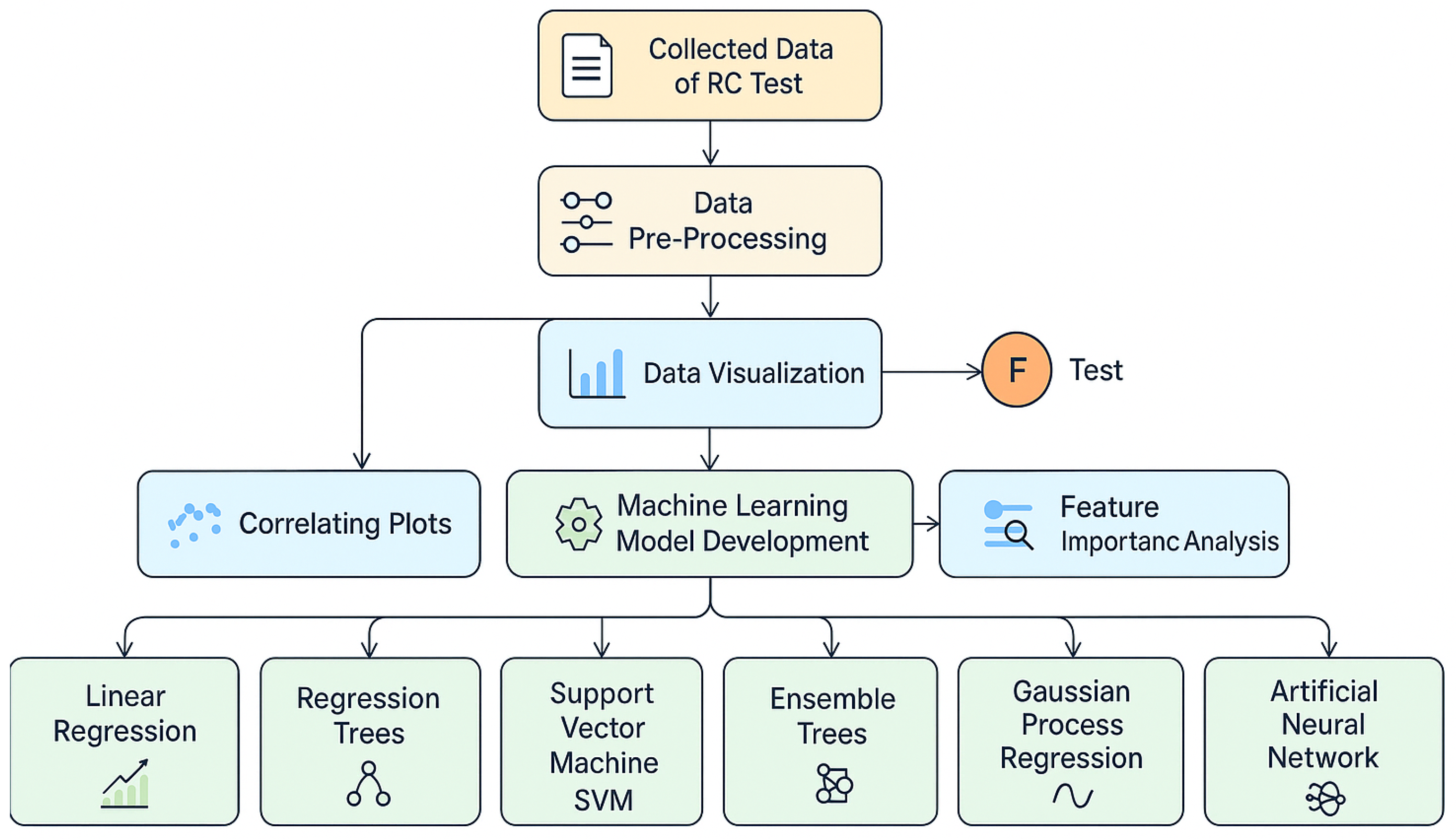
Figure 1. Methodology structure.
Buildings 15 04188 g001
Figure 2. Shear modulus (G) distribution versus numerical inputs.
Buildings 15 04188 g002aBuildings 15 04188 g002b
Figure 3. Damping (D) versus major input variables.
Buildings 15 04188 g003aBuildings 15 04188 g003b
Figure 4. Labeled diagram of decision tree node types: root, internal, and leaf.
Buildings 15 04188 g004
Figure 5. Feature importance (F-test–shear modulus).
Buildings 15 04188 g005
Figure 6. Feature importance (F-test–damping).
Buildings 15 04188 g006
Figure 7. Comparison between the machine learning models for shear modulus (G) prediction.
Buildings 15 04188 g007
Figure 8. Partial dependence of shear modulus G (MPa) on normalized e 0 , w , σ 0 , and γ .
Buildings 15 04188 g008
Figure 9. Comparison between the machine learning models for Damping (D) prediction.
Buildings 15 04188 g009aBuildings 15 04188 g009b
Figure 10. Partial dependence of the damping ratio D (%) on normalized e 0 , w , σ 0 , and γ .
Buildings 15 04188 g010
Figure 11. Model-to-standards integration framework.
Buildings 15 04188 g011
Table 1. Summary of collected data.
Data
Type
Data AttributeDescriptionBrief DefinitionNumber/ Categorical
Inputs z Depth of sample (m)Depth below ground levelNumber
G s Specific gravityRelative density of solids to waterNumber
ρ Soil density (Mg/m3)Bulk (wet) density of soilNumber
L L Liquid limit (%)Moisture content at plastic–liquid transitionNumber
P I Plasticity index (%)Moisture range for plastic behavior ( L L P L )Number
w Water content (%)Mass of water over dry soil massNumber
USCS-CHUSCS classification codeUSCS classifications for clay, silt, or sand typesCategorical
USCS-CLUSCS classification codeCategorical
USCS-MH-OHUSCS classification codeCategorical
USCS-SCUSCS classification codeCategorical
USCS-OHUSCS classification codeCategorical
USCS-ML-OLUSCS classification codeCategorical
USCS-CL-CHUSCS classification codeCategorical
USCS-CL-MLUSCS classification codeCategorical
e0Initial void ratioVoids-to-solids ratio at startNumber
σ′pPreconsolidation pressure (kPa)Maximum past effective vertical stressNumber
OCR*Overconsolidation ratio σ p / σ 0 Number
σ′0Test confining pressure (kPa)Applied an effective confining pressure in the testNumber
ϒlElastic threshold (%)Strain at the onset of elastic behaviorNumber
ϒvVolumetric threshold (%)Strain at the onset of significant volumetric changeNumber
ϒShear strain amplitude induced during RC or CTS test (%)Imposed shear strain during RC/CTSNumber
OutputGShear modulus measured during RC or CTS test (kPa)Stiffness measured in RC/CTS (small–medium strain)Number
DDamping ratio measured during RC or CTS test (%)Hysteretic energy dissipation measured in RC/CTSNumber
Table 2. Summary of statistical analysis.
MedianMeanStd. DeviationRangeMinimumMaximum
z [m]11.8715.0111.0348.301.4549.75
GS [-]2.702.700.060.552.322.87
ρ [Mg/m3]2.022.000.140.901.302.19
LL [%]45.0048.4218.31140.0024.00164.00
PI [%]24.0025.3311.3980.004.0084.00
w [%]26.0628.3213.42113.4016.40129.80
e0 [-]0.630.680.292.060.402.46
σ′p [kPa]310.00310.99187.57870.0030.00900.00
OCR* [-]2.502.992.268.401.009.40
σ′0 [kPa]200.00227.56125.72490.0050.00540.00
ϒl [%]0.000.010.000.024.5 × 10−40.02
ϒv [%]0.030.050.050.340.010.35
ϒ [%]0.010.040.090.631.9 × 10−50.63
G [MPa]70.4284.2254.79288.493.54292.02
D (%)3.284.803.8121.670.9222.59
Table 3. Performance measures of machine learning models for predicting shear modulus.
Model TypeSpecificationsRMSEMSER-Squared
Linear RegressionLinear30,612.70937,137,444.500.69
Interactions Linear20,238.44409,594,453.800.86
Robust Linear32,885.611,081,463,145.000.64
Regression TreeFine Tree7292.7153,183,572.950.98
Medium Tree9031.6781,571,082.400.97
Coarse Tree15,359.48235,913,499.000.92
SVMLinear SVM31,892.971,017,161,800.000.66
Quadratic SVM18,001.66324,059,642.900.89
Cubic SVM16,174.61261,617,886.700.91
Fine Gaussian SVM10,027.04100,541,590.300.97
Medium Gaussian SVM16,193.21262,220,042.700.91
Coarse Gaussian SVM28,942.11837,645,622.200.72
Ensemble TreeBoosted Trees11,600.99134,582,891.800.96
Bagged Trees7208.5151,962,677.320.98
Gaussian Process RegressionSquared Exponential GPR11,252.71126,623,457.000.96
Matern 5/2 GPR8226.0367,667,600.970.98
Exponential GPR2263.035,121,318.410.99
Rational Quadratic GPR2424.735,879,291.410.99
Neural NetworkNarrow Neural Network9994.0399,880,577.320.97
Medium Neural Network6918.2747,862,394.710.98
Wide Neural Network3935.1115,485,057.040.99
Bilayered Neural Network7940.9363,058,396.100.98
Trilayered Neural Network8127.1766,050,865.960.98
KernelSVM Kernel56,215.573,160,190,262.00−0.05
Least Squares Regression Kernel30,263.23915,863,154.300.70
Table 4. Performance measures of machine learning models for predicting damping ratio.
Model TypeSpecificationsRMSEMSER-Squared
Linear RegressionLinear2.455.990.60
Interactions Linear2.415.790.61
Robust Linear3.3110.940.27
Regression TreeFine Tree1.572.470.83
Medium Tree1.572.470.83
Coarse Tree1.662.750.82
SVMLinear SVM2.646.960.53
Quadratic SVM2.044.170.72
Cubic SVM6.3940.83−1.73
Fine Gaussian SVM1.973.860.74
Medium Gaussian SVM1.853.420.77
Coarse Gaussian SVM2.405.770.61
Ensemble TreeBoosted Trees1.502.260.85
Bagged Trees1.462.140.86
Gaussian Process RegressionSquared Exponential GPR1.702.880.81
Matern 5/2 GPR1.682.830.81
Exponential GPR1.662.750.82
Rational Quadratic GPR1.682.830.81
Neural NetworkNarrow Neural Network1.903.600.76
Medium Neural Network1.813.260.78
Wide Neural Network1.712.930.80
Bilayered Neural Network2.124.490.70
Trilayered Neural Network1.813.280.78
KernelSVM Kernel3.9915.95−0.07
Least Squares Regression Kernel3.5912.870.14
Disclaimer/Publisher’s Note: The statements, opinions and data contained in all publications are solely those of the individual author(s) and contributor(s) and not of MDPI and/or the editor(s). MDPI and/or the editor(s) disclaim responsibility for any injury to people or property resulting from any ideas, methods, instructions or products referred to in the content.