A Novel Active Learning Method Combining Adaptive Support Vector Regression and Monte Carlo Simulation for Structural Reliability Assessment

Abstract

Structural reliability analysis remains challenging when only a limited number of calls to expensive numerical models, such as finite-element solvers, are acceptable. In recent years, active learning (AL) metamodel methods have attracted considerable attention as they offer an efficient and accurate solution for reliability assessment. A common feature of these methods is that they initially construct a low-accuracy metamodel, which is then iteratively updated by sequentially enriching the training dataset according to specific learning functions. This paper proposes a novel active learning reliability method (ALRM) that combines the advantages of support vector regression (SVR) and Monte Carlo simulation (ASVR-MCS). A learning function based on the penalty function method is developed to identify optimal sampling points. To validate the efficacy and versatility of ASVR-MCS, it is applied to four representative structural reliability problems, which are characterized by multiple design points, disjoint failure regions, and implicit performance functions. The performance of ASVR-MCS is systematically compared with that of two other well-established ALRMs, i.e., AK-MCS (based on Kriging) and ASVM-MCS (based on Support Vector Machine). The numerical results demonstrate that the proposed ASVR-MCS method not only achieves high computational efficiency but also exhibits wider applicability in structural reliability analysis.

1. Introduction

Structural reliability analysis aims to compute the probability of failure-related events in engineering systems [1,2]. Probabilistic assessment is essential for ensuring structural safety when accounting for the uncertainties of input parameters [3,4,5,6]. For a probabilistic system of practical interest, uncertainties such as material properties, the size of structural elements, loads, and environmental factors are represented by an N-dimensional random vector $\mathbf{X}$ with a continuous joint probability density function $f_{\mathbf{X}}\left(\mathbf{x}\right)$, where $\mathbf{x}\in {\mathbb{R}}^N$ is a realization of the random variables $\mathbf{X}$ [7,8,9]. Failure is defined by a performance function $G\left(\mathbf{x}\right)$, generally determined by a combination of system responses and allowable thresholds, representing one or a composite of multiple failure modes. The physical meaning of $G\left(\mathbf{x}\right)$ depends on the specific problem under consideration. The failure probability can then be expressed as a multiple integral on the probabilistic space:

$$P_f={\int }_{{\mathbb{R}}^N}{I}_F\left(\mathbf{x}\right)f_{\mathbf{X}}\left(\mathbf{x}\right)d\mathbf{x},$$

(1)

where $I_F\left(\mathbf{x}\right)$ is the indicator function of failure domain $F=\left\{\mathbf{x}\right|G\left(\mathbf{x}\right)\le 0\}$, i.e., $I_F\left(\mathbf{x}\right)=1$ if $\mathbf{x}\in F$, and $I_F\left(\mathbf{x}\right)=0$ otherwise.

An analytical solution to Equation (1) is generally infeasible, especially when the performance function cannot be expressed as explicit, closed-form function of the input variables [10,11,12]. A popular technique for accessing structural reliability is the metamodel method (also known as the surrogate model method). Metamodel approaches seek to construct an approximate model to substitute the complicated real limit state function (LSF) based on a strategic design of experiments (DoE). However, the number of DoEs required is a critical issue in constructing metamodels. Consequently, adaptive metamodels have been proposed to reduce the size of DoEs. Various types of adaptive metamodels have been investigated, including moving least squares [3], polynomial chaos expansions (PCEs) [13,14], Kriging [5,15,16,17], artificial neural networks (ANNs) [18,19], SVM [20,21,22,23,24,25], and SVR [26,27].

It is worthwhile to mention the ALRMs, represented by AK-MCS [5], which combine an adaptive Kriging metamodel and Monte Carlo simulation. The efficiency of these ALRMs has been validated. They require only a few hundred or fewer number of calls to the true LSF while achieving accurate results compared to pure simulation methods, even in cases involving multiple most probable points (MPPs) and high nonlinearity [5,15,16]. ALRMs are powerful and promising due to their skillful combination of simulation methods and adaptive metamodels, specifically for three reasons: (1) The region approximated by the metamodel is restricted to a limited area covered by samples generated by the simulation method, avoiding attention being paid to regions with very low probability densities. (2) DoEs are sequentially enriched based on a learning function that integrates available information from the sample population and the updating metamodel. (3) The search for optimal points is limited to a discrete sample population, eliminating the need for expensive optimization algorithms. However, existing research on ALRMs has mostly focused on the Kriging metamodel [15,16,28,29,30,31,32,33], owing to its built-in prediction variance, which facilitates the construction of learning functions to guide the selection of subsequent training samples [19]. It should be noted that the Kriging metamodel may become less efficient when dealing with high-dimensional and highly nonlinear problems [7,34]. As a consequence, other metamodels such as PCE [35,36], ANN [19,34], RBF [37], SVM [20], and SVR [27,38,39] have been adopted to develop active learning methods for structural reliability analysis.

While the aforementioned metamodels each possess distinct advantages, they also exhibit certain limitations. For instance, ANNs are often susceptible to under- or overfitting. PCE can suffer from the “curse of dimensionality”, which restricts its applicability to low- or moderate-dimensional problems. Meanwhile, Kriging and RBF may struggle to accurately capture highly nonlinear LSFs. In contrast, SVM and SVR are grounded in statistical learning theory, which endows them with strong capabilities for handling nonlinearity and mitigating overfitting, often leading to superior generalization performance. These characteristics make SVR a particularly suitable choice for structural reliability analysis. The optimization strategy of SVM is to maximize the margin between two hyperplanes that separate the two classes of linearly separable training points, and its nonlinearly separable ability is extended by using the kernel mapping from the input space to a higher-dimensional space. SVR is an extension of SVM that demonstrates excellent performance in capturing nonlinearity by means of kernel mapping [40]. By balancing the minimization of error over training pairs and the complexity of the trained model, SVR aims to find a linear regression relationship among sparse input–output pairs in the original space or the mapping space (feature space). Compared to SVM, SVR is more informative as it is a regression model that fully exploits the response values, not just the sign of the performance function at a given input sample point [26]. Therefore, SVR is selected as the primary metamodel in this paper. The objective of this work is to propose a novel efficient reliability method: ASVR-MCS.

The effective application of SVR within ALRMs hinges on addressing two primary challenges: (1) developing an appropriate learning function that balances global exploration with local exploitation to train the metamodel effectively [38,41], and (2) establishing a robust stopping criterion that accurately monitors metamodel convergence, thereby avoiding either premature termination or unnecessary computational waste [39]. Concerning the learning function, a critical requirement is the construction of a reliable prediction variance, as standard SVR does not inherently provide uncertainty estimates. To bridge this gap, various methods have been proposed, such as those based on maximum Euclidean distance [20,27] and approaches utilizing cross-validation and Jackknifing [19,39]. However, distance-based variances primarily ensure that new samples are positioned far from existing DoEs and may not reflect the prediction uncertainty at candidate points [27,42]. Conversely, while prediction variances often demonstrate superior performance, they do not necessarily guarantee an even distribution of training samples. To overcome the limitations of both, the present study adopts a hybrid variance metric that integrates the distance to existing DoEs with the prediction variance at candidate samples. Furthermore, existing adaptive SVR methods frequently employ ratio-type learning functions (e.g., the U-function), which can lead to the selection of samples precisely on the LSF regardless of their prediction uncertainty [5,20,27]. This may result in an inefficient allocation of computational resources to samples that minimally enhance metamodel accuracy [20]. To mitigate this issue, we propose a novel weighted penalty learning function that incorporates the distance from a candidate sample to the predicted LSF in a linearly combined form. Regarding the stopping criterion, many existing studies rely on a single-indicator approach, often based on the stability of failure probability estimates [27,42]. Such a criterion can be sensitive to statistical noise. Alternative metrics, including the root mean square error (RMSE), the coefficient of determination ($R^2$), and the mean squared error (MSE), can also be employed to assess metamodel accuracy [43,44]. In this work, a composite stopping criterion is introduced that simultaneously considers the global convergence trend toward the true LSF and the local fitting accuracy of the metamodel. This integrated strategy fosters a more stable and robust active learning process.

The performance of the proposed method is compared with two other ALRMs based on the Kriging and SVM metamodels. Numerical examples verify that the proposed method leverages the advantages of SVR and MCS, providing accurate and efficient results for the reliability analysis of practical engineering structures. The remainder of this paper is organized as follows: First, a brief introduction to SVR is presented. Then, a novel pool-based adaptive metamodel method ASVR-MCS is proposed based on the AK-MCS framework. Subsequently, four numerical examples are given to compare the capability of handling various LSFs with two other existing ALRMs. Finally, conclusions are drawn.

2. The Proposed Method: ASVR-MCS

This section proposes a novel ALRM named ASVR-MCS that combines adaptive support vector regression with Monte Carlo simulation. Firstly, a brief introduction to SVR is presented; interested readers may refer to [40] for more details. Then, the framework of the proposed method adopting the active learning strategy is developed.

2.1. Support Vector Regression

Given m sets of training points $\{({\mathbf{x}}_i,y_i),i=1,2,\dots ,m\}$, the vector ${\mathbf{x}}_i\in {\mathbb{R}}^N$ is the input and the target value $y_i\in \mathbb{R}$ is the output. Since the input variables had been normalized within the physical problem formulation, they were used directly without scaling or transformation (i.e., no feature preprocessing was required). SVR aims to find a relationship between the input space ${\mathbb{R}}^N$ and the output space $\mathbb{R}$. Linear SVR can be applied to find a function with the form

$$\tilde{G}\left(\mathbf{x}\right)={\mathbf{w}}^{\mathrm{T}}\mathbf{x}+b,$$

(2)

where $\mathbf{w}$ is the weight vector perpendicular to hyperplane $\tilde{G}\left(\mathbf{x}\right)=0$ and b is a bias parameter. The model parameters are obtained by minimizing the flatness of the function while restricting the prediction deviation to be below a tolerance threshold $\epsilon$, i.e.,

$$\begin{array}{c}minJ\left(\mathbf{w}\right)={\displaystyle \frac{1}{2}}{∥\mathbf{w}∥}^2\\ \mathrm{s}.\mathrm{t}.\forall i:\left|y_i-\left({\mathbf{w}}^{\mathrm{T}}{\mathbf{x}}_i+b\right)\right|\le \epsilon \end{array}.$$

(3)

Since such a function may not exist, non-negative slack variables ${\xi }_i^{\pm }$ are introduced to soften the constraints for each training point. Equation (3) can be reformulated as

$$\begin{array}{c}\min J(\mathbf{w},{\xi }_i^{+},{\xi }_i^{-})={\displaystyle \frac{1}{2}}{∥\mathbf{w}∥}^2+C{\displaystyle \sum _{i=1}^m}({\xi }_i^{+}+{\xi }_i^{-})\\ \mathrm{s}.\mathrm{t}.\left\{\begin{array}{c}\forall i:y_i-({\mathbf{w}}^{\mathrm{T}}{\mathbf{x}}_i+b)\le \epsilon +{\xi }_i^{+}\\ \forall i:({\mathbf{w}}^{\mathrm{T}}{\mathbf{x}}_i+b)-y_i\le \epsilon +{\xi }_i^{-}\\ \forall i:{\xi }_i^{+},{\xi }_i^{-}\ge 0\end{array}\right.\end{array},$$

(4)

where C is the box constraint parameter that controls the trade-off between minimizing the complexity of the trained model and the amount of fitting error exceeding $\epsilon$. This optimization problem is more easily solved by converting the corresponding expression in Equation (4) into its Lagrange dual form:

$$\begin{array}{c}L({\alpha }_i,{\alpha }_i^{*})={\displaystyle \frac{1}{2}}{\displaystyle \sum _{i=1}^m}{\displaystyle \sum _{j=1}^m}\left({\alpha }_i-{\alpha }_i^{*}\right)\left({\alpha }_j-{\alpha }_j^{*}\right){\mathbf{x}}_i^{\mathrm{T}}{\mathbf{x}}_j\\ +\epsilon {\displaystyle \sum _{i=1}^m}\left({\alpha }_i+{\alpha }_i^{*}\right)+{\displaystyle \sum _{i=1}^m}{y}_i\left({\alpha }_i^{*}-{\alpha }_i\right)\\ \mathrm{s}.\mathrm{t}.{\displaystyle \sum _{i=1}^m}\left({\alpha }_i-{\alpha }_i^{*}\right)=0\mathrm{and}\forall i:{\alpha }_i,{\alpha }_i^{*}\in [0,C]\end{array},$$

(5)

where ${\alpha }_i$ and ${\alpha }_i^{*}$ are the non-negative Lagrange multipliers. The solutions to the primal problem in Equation (4) and its dual problems in Equation (5) are equivalent because the Karush–Kuhn–Tucker conditions are satisfied. In the dual formulation, the weight vector $\mathbf{w}$ can be described analytically as $\mathbf{w}={\displaystyle \sum _{i=1}^m}\left({\alpha }_i-{\alpha }_i^{*}\right){\mathbf{x}}_i$. Then, the regression function $\tilde{G}\left(\mathbf{x}\right)$ can be expressed as

$$\tilde{G}\left(\mathbf{x}\right)=\sum _{i=1}^m\left({\alpha }_i-{\alpha }_i^{*}\right){\mathbf{x}}_i^{\mathrm{T}}\mathbf{x}+b.$$

(6)

The nonlinear regression model is obtained by mapping the input variables $\mathbf{x}$ to a high-dimensional space via a transformation function $\varphi \left(\mathbf{x}\right)$. Kernel functions $K({\mathbf{x}}_i,{\mathbf{x}}_j)$ are introduced to reduce the computational burden of mapping operations, as they directly calculate the inner product of the transformed values, i.e., $K({\mathbf{x}}_i,{\mathbf{x}}_j)={\varphi }^{\mathrm{T}}\left({\mathbf{x}}_i\right)\varphi \left({\mathbf{x}}_j\right)$. Nonlinear SVR is developed by substituting the kernel function $K({\mathbf{x}}_i,{\mathbf{x}}_j)$ for the inner product ${\mathbf{x}}_i^{\mathrm{T}}\mathbf{x}$ in Equation (6):

$$\tilde{G}\left(\mathbf{x}\right)=\sum _{i=1}^m\left({\alpha }_i-{\alpha }_i^{*}\right)K(\mathbf{x},{\mathbf{x}}_i)+b.$$

(7)

Several models can be used to define kernel function, such as the polynomial, sigmoid, or Gaussian kernels. This paper adopts the widely used Gaussian kernel in the context of SVM. The SVR technique was implemented using the MATLAB R2019a Statistics and Machine Learning Toolbox, with default configurations for hyperparameter grid ranges and random-seed handling, ensuring reproducibility under standard platform settings.

2.2. Active Learning Reliability Method: ASVR-MCS

The straightforward extension of SVR to the AL framework of AK-MCS is restricted because SVR cannot measure the prediction error directly. To solve this issue, this paper introduces two existing learning functions [19,20] and a novel learning function based on the concept of weighting penalty. Additionally, a modified stopping criterion referring to the stability of the failure region is developed to stop active learning iteration.

2.2.1. Learning Function

In active learning iteration, the core procedure is to identify the next best sample. Bichon et al. [17] proposed an adaptive sequential sampling method referred as efficient global reliability analysis (EGRA), which adopts the expected feasibility function ($EFF$) to indicate how well a sample point is expected to locate in the vicinity of the limit state boundary. Since only the sign of the performance function is crucial in numerical simulation, Echard et al. [5] proposed a learning function named U to measure the potential risk of untried points crossing the predicted LSF. The expression is given as

$$U\left(\mathbf{x}\right)={\displaystyle \frac{\left|\tilde{G}\left(\mathbf{x}\right)\right|}{{\sigma }_{\tilde{G}}\left(\mathbf{x}\right)}},$$

(8)

where $\tilde{G}\left(\mathbf{x}\right)$ and ${\sigma }_{\tilde{G}\left(\mathbf{x}\right)}$ are the metamodels’ predicted response and variance, respectively. The successful application of these functions is attributed to the predicted variance of Kriging, which guides the selection of sequentially added samples. However, SVR does not provide a direct mechanism for measuring the variance, making these classical learning functions inapplicable. To address this, three learning functions are adopted for ASVR-MCS: these are the function $L(·)$ proposed by Pan et al. [20], the function ${\psi }_{\mathrm{m}}(·)$ studied by Xiao et al. [19], and a novel function $P(·)$ proposed herein.

I.

The modified classical learning function $L(·)$

Pan et al. [20] developed ASVM-MCS. They considered that optimal points selected by a learning function should simultaneously be (1) as close as possible to the boundary of the SVM classifier, and (2) far away from existing training samples. Therefore, the learning function $L(·)$ was proposed as a balance between these two features. $L(·)$ can be regarded as a modification of the classical learning function $U(·)$ and is defined as

$$L\left(\mathbf{x}\right)={\displaystyle \frac{\left|\tilde{G}\left(\mathbf{x}\right)\right|}{D\left(\mathbf{x}\right)}}.$$

(9)

Equation (9) replaces the Kriging variance ${\sigma }_{\tilde{G}\left(\mathbf{x}\right)}$ in Equation (8) with the maximum Euclidean distance $D\left(\mathbf{x}\right)$ from the candidate point to its nearest existing training sample. This distance variance is calculated by

$$D\left(\mathbf{x}\right)=∥\mathbf{x}-\xi \left(\mathbf{x}\right)∥,$$

(10)

where $\xi \left(\mathbf{x}\right)$ is the closest point to the untried point $\mathbf{x}$ in the existing training set. This function requires no information about prediction variance and can be feasibly applied to the proposed ASVR-MCS algorithm.

II.

The mixed learning function ${\psi }_{\mathrm{m}}\left(\mathbf{x}\right)$

Xiao et al. [19] proposed an active learning reliability method to construct a back-propagation neural network for efficient reliability analysis. In their work, the predicted variance was calculated by using the cross-validation and Jackknifing approach. Cross-validation (CV) involves dividing the existing DoEs into $k_s$ CV subsets; then, the $k_s$ sub-training sampling set is obtained by removing one of the CV subsets from the complete sample set, allowing the $k_s$ sub-metamodels to be trained based on those sub-training sampling sets. Jackknifing estimates the prediction uncertainty by measuring the variability of the responses across the k sub-metamodels.

Xiao et al. [19] also proposed a mixture variance ${\sigma }_m^2\left(\mathbf{x}\right)$ in order to combine the advantages of $D\left(\mathbf{x}\right)$ and ${\sigma }_J^2\left(\mathbf{x}\right)$ by linear weighting. Consequently, a novel learning function ${\psi }_{\mathrm{m}}(·)$ was proposed by replacing the variance in function $U(·)$ with the mixture variance, and it was determined by

$${\psi }_{\mathrm{m}}\left(\mathbf{x}\right)={\displaystyle \frac{\left|\tilde{G}\left(\mathbf{x}\right)\right|}{{\sigma }_m^2\left(\mathbf{x}\right)}}={\displaystyle \frac{\left|\tilde{G}\left(\mathbf{x}\right)\right|}{(1-\alpha ){\overline{\sigma }}_J^2\left(\mathbf{x}\right)+\alpha \overline{D}\left(\mathbf{x}\right)}},$$

(11)

where $\alpha$ ranges from 0 to 1 is a weight coefficient, and $\overline{D}\left(\mathbf{x}\right)$ and ${\overline{\sigma }}_J^2\left(\mathbf{x}\right)$ are the results normalized by their maximum function value observed in candidate pool S, i.e., $\overline{D}\left(\mathbf{x}\right)={\displaystyle \frac{D\left(\mathbf{x}\right)}{{\displaystyle \underset{\mathbf{x}\in S}{max}}\left(D\left(\mathbf{x}\right)\right)}}$ and ${\overline{\sigma }}_J^2\left(\mathbf{x}\right)={\displaystyle \frac{{\sigma }_J^2\left(\mathbf{x}\right)}{{\displaystyle \underset{\mathbf{x}\in S}{max}}\left({\sigma }_J^2\left(\mathbf{x}\right)\right)}}$.

III.

The proposed weighting penalty learning function $P(·)$

The learning functions in Equations (8), (9) and (11) share a unified form, representing a trade-off between the predicted value and the predicted variance. It should be emphasized again that these functions aim to find points in the candidate pool with the highest probability of incorrect sign prediction. However, for points located on the predicted LSF (i.e., the prediction response $\tilde{G}\left(\mathbf{x}\right)=0$), the value of these learning functions is zero regardless of the variance, potentially leading to the selection of points that offer little improvement to the metamodel’s accuracy. To solve the issue, we first consider that the points with the largest variance located on the true LSF have the highest potential to improve the fitting accuracy of the metamodel. From an optimization perspective, we can construct an optimization problem with equality constraints to search for these points:

$$\begin{array}{c}{\mathbf{x}}^{*}=\arg \max \left({\sigma }_G^2\left(\mathbf{x}\right)\right)\\ \mathrm{s}.\mathrm{t}.G\left(\mathbf{x}\right)=0\end{array}.$$

(12)

Since the learning function is evaluated on an MCS population, it naturally avoids selecting the points with weak probability densities. In practical applications, we can use the predicted variance ${\tilde{\sigma }}_G^2\left(\mathbf{x}\right)$ and predicted response $\tilde{G}\left(\mathbf{x}\right)$ of the metamodel as substitutes for the real ones. The constrained condition $\tilde{G}\left(\mathbf{x}\right)=0$ is commonly implicit; thus, the objective function can be reconstructed using a penalty function by converting the maximum constrained optimization problem into the corresponding minimized unconstrained problem. Accordingly, a weighting penalty learning function is defined as

$$P\left(\mathbf{x}\right)={\displaystyle \frac{1}{{\overline{\sigma }}_G\left(\mathbf{x}\right)}}+c·\left|\overline{G}\left(\mathbf{x}\right)\right|,$$

(13)

where $\overline{G}\left(\mathbf{x}\right)$ and ${\overline{\sigma }}_G^2\left(\mathbf{x}\right)$ are the results of $\tilde{G}\left(\mathbf{x}\right)$ and ${\tilde{\sigma }}_G^2\left(\mathbf{x}\right)$ normalized by their maximum function values in the candidate pool, respectively; c is the penalty coefficient, which can be set to ${10}^1$∼${10}^4$ based on our computational results. This range balances exploration and exploitation in the learning process. Smaller values (<${10}^1$) lead to excessive exploration, while larger ones (>${10}^4$) cause premature convergence. Our preliminary studies reveal that within the range of (${10}^1$ to ${10}^4$), the penalty and variance terms contribute comparably, ensuring stable and efficient sampling near the limit-state surface. A more comprehensive study over additional numerical examples is needed to further determine the reasonable range of c. The variance $D\left(\mathbf{x}\right)$ ensures the selected samples are sufficiently far from existing points in the current training set in the input parameter space. The Jackknifing variance ${\sigma }_J^2\left(\mathbf{x}\right)$ measures the degree of difficulty or variation in predicting the response in the output space. Therefore, the mixture variance ${\sigma }_m^2\left(\mathbf{x}\right)$ comprehensively considers the available information about prediction uncertainty in both the input parameter and output response spaces, and we adopt it to estimate the prediction variance ${\tilde{\sigma }}_G^2\left(\mathbf{x}\right)$ in this paper. The weight coefficient is set to $\alpha =0.5$, as suggested by Xiao et al. [19]. The learning function $P(·)$ represents an overall consideration of the predicted response and variance but emphasizes finding the points that improve the accuracy of the metamodel, rather than focusing on finding those whose states are easily misclassified.

2.2.2. Stop Criteria

The stop criteria are employed to terminate the update of the adaptive metamodel. Overly relaxed criteria yield a low-accuracy metamodel, while overly conservative ones lead to adding unnecessary samples with little improvement in accuracy. Considering the stability of the failure domain, two stopping criteria modified from [45] are developed, which are defined as follows:

$${\delta }_1={\displaystyle \frac{\left|{\widehat{P}}_f^{\left(j\right)}-{\widehat{P}}_f^{(j-1)}\right|}{{\widehat{P}}_f^{\left(j\right)}}}<{\epsilon }_1,$$

(14)

$${\delta }_2=\sum _{i=1}^{N_s}{\displaystyle \frac{\left|\mathrm{sign}({\tilde{G}}^{(j-1)}\left({\mathbf{x}}_{\mathrm{s}}^i\right))-\mathrm{sign}({\tilde{G}}^{\left(j\right)}\left({\mathbf{x}}_{\mathrm{s}}^i\right)\right|}{N_F^{\left(j\right)}}}<{\epsilon }_2,$$

(15)

where ${\widehat{P}}_f^{\left(j\right)}$ is estimated failure probability at the $j^{\mathrm{th}}$ iteration of the proposed method; ${\tilde{G}}^{\left(j\right)}$ is the metamodel constructed at the $j^{\mathrm{th}}$ iteration; $N_s$ is the total number of samples in candidate pool $S=\{{\mathbf{x}}_{\mathrm{s}}^i,i=1,\dots ,N_s\}$; and $N_F^{\left(j\right)}$ denotes the number of failed samples in population S. The active learning process aims at training a comparatively exact metamodel to substitute the true LSF at the region covered by population S. The first criterion reflects the global trend of how well the predicted LSF coincides with the true one. The second criterion relates to the proportion of sign changes in the metamodel predictions for the candidate sample pool between two successive iterations, accounting for fitting accuracy in local areas. Convergence is assumed if both criteria are simultaneously satisfied in two adjacent iterations. The thresholds ${\epsilon }_1$ and ${\epsilon }_2$ are chosen to balance computational efficiency with the metamodel accuracy. Specifically, selecting smaller values for ${\epsilon }_1$ and ${\epsilon }_2$ would lead to an overly conservative stopping condition. This could result in an unnecessary increase in the size of the DoEs, requiring more samples to be added with little accuracy improvement for the metamodel. Conversely, larger threshold values would relax the stopping condition excessively. While this reduces the number of samples added into the DoEs and LSF evaluations, it risks compromising the accuracy of the metamodel. Based on the reference values [45,46,47] and our practical experience, the thresholds ${\epsilon }_1$ and ${\epsilon }_2$ are selected as 0.001 and 0.01, respectively. However, the optimal values may be adjusted depending on the specific accuracy and efficiency requirements of a given application.

For practical issues related to computational resource limitations, the proposed method will be forced to stop if the total number of calls to the true performance function reaches a threshold $N_{\mathrm{call}}^{max}$.

2.2.3. Implementation of the Proposed Method

The proposed method ASVR-MCS is an extension of AK-MCS that constructs a sequential sampling SVR instead of Kriging. At first, a sample population generated by crude MCS is regarded as a candidate pool rather than being directly evaluated on the true LSF. A low-accuracy SVR metamodel is constructed based on an initial DoE composed of a small set of samples. The metamodel is then dynamically updated by enriching the training set with the most promising point from the candidate pool, identified using a learning function at each iteration. The active learning process continues until the stopping criteria are satisfied. The final refined SVR metamodel is considered accurate enough to substitute for the true LSF. Finally, the MCS estimator uses the metamodel to classify the state (safe or failure) of the sample population and obtains a fairly accurate estimation of failure probability. The iterative process of the ASVR-MCS is described as follows:

Step 1. Generate $N_s$ Monte Carlo samples following the PDF of random variables. This population is denoted as $S=\{{\mathbf{x}}_{\mathrm{s}}^i,i=1,\dots ,N_s\}$, representing the initial simulation region for the metamodel SVR. Note that S is a candidate pool of the active learning process, and none of the samples are labeled by the true limit state function at this stage.

Step 2. Generate the initial DoEs using Latin Hypercube Sampling (LHS). In order to capture the global behavior of the model response [20,29], LHS is employed to make the initial DoE as uniform as possible. The distribution bounds of the initial DoE are determined by multiplying the standard deviation of the random variables by a factor of five. The principle of active learning is to start with a small set of training pairs due to the necessity of problem complexity. Thus, the sample size of the initial DoE is selected as $max\{15,N+2\}$, where N is the dimension of the probabilistic system.

Step 3. Train the metamodel SVR based on the current DoE. The metamodel SVR is trained by implementing the Statistics and Machine Learning Toolbox in MATLAB R2019a. The Gaussian kernel is selected. The selection of the scale of Gaussian kernel is an ongoing topic [20]. In this work, the value of the scale factor is automatically determined by the software’s heuristic procedure in the first step and kept constant thereafter, a strategy also adopted in [21].

Step 4. Select the optimal points according to the learning function. The composite learning function is employed in this stage. The learning function is evaluated on all points of population S to identify the next best points:

$${\mathbf{x}}^{*}=\underset{{\mathbf{x}}_{\mathrm{s}}^i\in S}{arg}min\left(F\left({\mathbf{x}}_{\mathrm{s}}^i\right)\right),$$

where $F(·)$ is the learning function.

Step 5. Check the stop criteria for active learning. The stop criteria are used to determine whether the updated metamodel is sufficiently accurate to terminate the active learning process. If the proposed stopping criterion is satisfied, the SVR metamodel is considered sufficiently accurate to replace the true LSF to label the sign of S, and the procedure proceeds to Step 6. If the stop condition is not met, the optimal point identified in the last step will be evaluated on the true performance function.The algorithm goes back to Step 3 to rebuild the new SVR metamodel with the updated training set.

Step 6. Calculate ${\widehat{P}}_f$ and the coefficient of variation $\mathrm{Cov}\left({\widehat{P}}_f\right)$. The obtained metamodel SVR is used to estimate ${\widehat{P}}_f$ and its coefficient of variation (Cov) according to MCS estimator [48]. If $\mathrm{Cov}\left({\widehat{P}}_f\right)$ is larger than an acceptable level ${\delta }_{\mathrm{tol}}$, meaning that the estimated value of ${\widehat{P}}_f$ is not accurate enough, S is enriched with another $N_s$ points generated from the Monte Carlo population. The methods returns to Step 4 and the active learning process restarts until the stop condition is satisfied again.

Step 7. End of the proposed method. If $\mathrm{Cov}\left({\widehat{P}}_f\right)$ is lower than ${\delta }_{\mathrm{tol}}$, the ASVR-MCS terminates, and an accurate estimate of ${\widehat{P}}_f$ is obtained.

The contributions of the proposed method lie in two key aspects: (1) Learning function: Unlike ratio-based forms (e.g., the U-function), our proposed function adopts a linear combination form that incorporates the distance from a candidate sample to the predicted LSF. This approach avoids selecting samples exactly on the LSF—a scenario where ratio-based functions can yield a zero value regardless of prediction uncertainty, thus wasting computational resources on samples that contribute minimally to metamodel accuracy. (2) Stopping criteria: The proposed criteria integrate both global convergence trends toward the true LSF and local metamodel fitting accuracy. This dual focus promotes a more stable and robust active learning process compared to methods that rely on a single metric.

Remark: It should be noted that the MCS is employed solely to generate a candidate sample pool in the proposed method. The key of the method lies in the subsequent active learning process, which adaptively selects the most informative samples from this pool to train the metamodel. This strategy ensures that only a small number of samples (i.e., a minimal number of LSF calls) is required to construct an accurate surrogate. Once the metamodel is built, the failure probability can be estimated with high efficiency, as it involves evaluating the fast-running metamodel instead of the original, computational expensive performance function. For problems with a large N, the adaptive nature of the active learning algorithm effectively controls the number of necessary LSF calls. Therefore, the total computational cost remains low, and a significant improvement in efficiency is achieved.

3. Numerical Examples

This section investigates four low-to-moderate-dimensional examples with multiple points, disjoint failure regions, or implicit expressions. The performance of the proposed method is compared with two other popular ALRMs: AK-MCS [5] and ASVM-MCS [20]. For a fair comparison, all ALRMs use the same strategies for generating initial DoEs and the same convergence criteria in Equations (14) and (15).

For all examples, the involved parameters of the ALRMs are specified as follows unless stated otherwise. The target coefficient of variation is set to be 0.05, and the maximum number of calls $N_{\mathrm{call}}^{max}$ to the performance function is set to be 300. The initial DoEs were generated using LHS within the region $\left[\mu \pm 5\sigma \right]$, where $\mu$ and $\sigma$ are the mean and standard deviation of the input random variables, respectively. The size of initial DoE is set to $max\left\{15,N+2\right\}$. A candidate sample pool of size ${10}^5$ was also created via MCS from the definition domain of the input random variables. Both the initial DoE and the candidate pool were generated in MATLAB R2019a, with the random seed controlled by the built-in random number generator. To reduce the uncertainty of the initial DoE and candidate sample pool, all ALRM algorithms were run 30 times. The efficiency and accuracy of AK-MCS, ASVM-MCS, and the proposed method ASVR-MCS were compared using several indicators: the total number of calls to LSF $N_{\mathrm{call}}$, the coefficient of variation $\mathrm{Cov}\left({\widehat{P}}_f\right)$ of the estimated failure probability ${\widehat{P}}_f$, and the relative error ${\epsilon }_{\mathrm{r}}$ between ${\widehat{P}}_f$ and the reference value.

3.1. Example One

The first example, taken from [49], is a series system with four branches. Its performance function is given by

$$G(x_1,x_2)=min\left\{\begin{array}{c}3+0.1{(x_1-x_2)}^2-(x_1+x_2)/\sqrt{2}\\ 3+0.1{(x_1-x_2)}^2+(x_1+x_2)/\sqrt{2}\\ (x_1-x_2)+7/\sqrt{2},(x_2-x_1)+7/\sqrt{2}\end{array}\right\},$$

(16)

where the two random variables $x_1$ and $x_2$ follow independent standard normal distributions.

The reference solution is obtained via MCS with a population size of ${10}^6$.

Table 1. Comparisons of results for Example 1.

Method	MCS	AK-MCS	ASVM-MCS	Proposed Method: ASVR-MCS
				$\mathit{L}$	${\mathit{\psi }}_{\mathrm{m}}$	$\mathit{P}$
${\widehat{P}}_f$	$2.244\times {10}^{-3}$	$2.203\times {10}^{-3}$	$1.968\times {10}^{-3}$	$2.119\times {10}^{-3}$	$2.090\times {10}^{-3}$	$2.173\times {10}^{-3}$
$N_{\mathrm{call}}$	$1.0\times {10}^6$	41.9	93.9	46.1	48.8	54.3
$\mathrm{Cov}\left({\widehat{P}}_f\right)$	-	4.87%	15.76%	7.66%	8.62%	5.7%
${\epsilon }_{\mathrm{r}}$	-	−1.9%	−12.3%	−5.6%	−6.9%	−3.2%

shows that ${\widehat{P}}_f$ calculated by AK-MCS and ASVR-MCS with different learning functions closely matches the MCS result. AK-MCS demonstrates higher efficiency, requiring fewer calls to the LSF than ASVR-MCS. However, ASVM-MCS requires over twice as many $N_{\mathrm{call}}$ as the other methods and exhibits lower accuracy, with average and maximum absolute relative errors of 12.3% and 50.2% over 30 runs. Figure 1 compares typical runs of the three ALRMs, illustrating the predicted LSF corresponding to the candidate pool and DoE distribution. It can be found that almost all of the optimal points identified by all methods lie near the true LSF. While AK-MCS (Figure 1a) and ASVR-MCS (Figure 1c) accurately capture all four branches of the true LSF within the MCS population region, ASVM-MCS (Figure 1b) completely misclassifies one branch. This discrepancy arises because SVM is a binary or multiclass classification model, which requires samples from both classes (i.e., samples from both the safe and failure regions) to define a decision boundary. Further observation of Figure 1b reveals that only a small number of DoE samples lie within the misclassified branch, while samples outside this branch are insufficient. Unsurprisingly, this leads to misfitting of the LSF for that branch. In contrast, Kriging and SVR are regression models that describe the relationship between response and input variables. For these models, the response values $G\left({\mathbf{x}}_i\right)$ of DoE samples are used to construct the metamodel, and this information helps locate the limit state function $G\left(\mathbf{x}\right)=0$. This example demonstrates that the ASVM-MCS algorithm may exhibit unstable fitting performance for problems involving multiple MPPs. Additionally, while ASVR-MCS is slightly less efficient and accurate than AK-MCS, its performance remains comparable.

Columns 5–7 of Table 1 present results for ASVR-MCS using three different learning functions. Among these, ASVR-MCS+P achieves the highest accuracy in estimating the failure probability. Figure 2 illustrates the active learning process for ASVR-MCS with different learning functions (using identical initial DoEs and candidate pools). Although the selected best points of all three methods lie near the true LSF, the added DoE samples of ASVR-MCS+P (Figure 2c) are more evenly distributed across the failure surface. In contrast, most DoE samples added for ASVR-MCS+L (Figure 2a) and ASVR-MCS+${\psi }_{\mathrm{m}}$ (Figure 2b) cluster near the MPPs. This clustering occurs because the probability density near the MPPs is relatively high, making it more likely to generate candidate points with predicted responses close to zero. Despite their low prediction variance, these points may be identified as optimal by the learning function L or ${\psi }_{\mathrm{m}}$. This example confirms that the learning function P is the most suitable choice for the proposed ASVR-MCS method.

3.2. Example Two

This example addresses a problem with infinitely disjoint responses. The performance function, investigated by Basudhar [22] (who proposed an SVM classifier to solve problems with discontinuous responses), is defined as

$$G(x_1,x_2)=x_2-\left|tan\left(x_1\right)\right|-1,$$

(17)

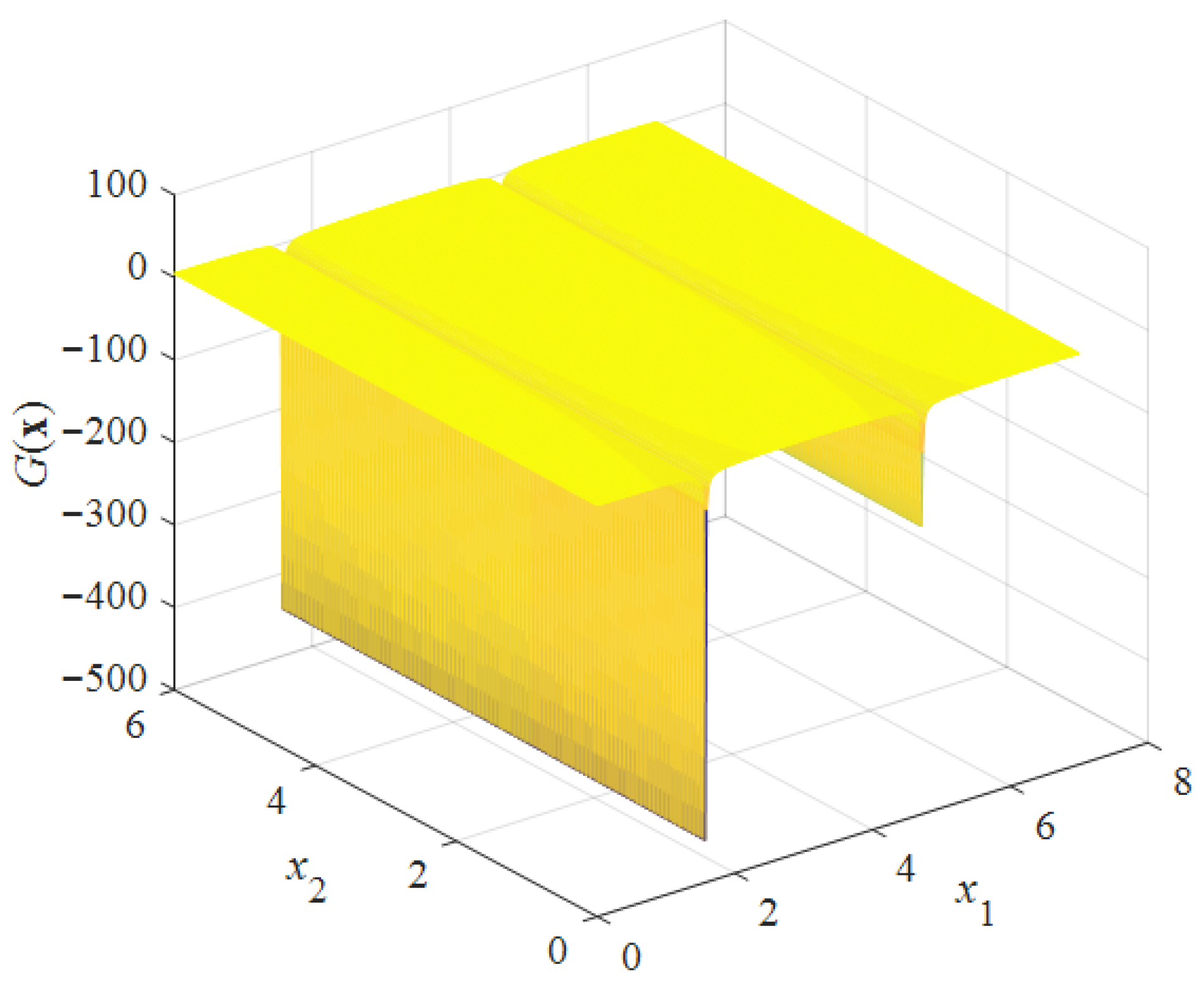
where $x_1$ and $x_2$ are two uniformly distributed variables over the intervals $[0,7]$ and $[0,6]$, respectively. Figure 3 depicts the performance function, which exhibits infinite discontinuity when $x_1$ approaches $\pi /2$ or $3\pi /2$.

This example is initialized with 30 space-filling Latin Hypercube Sampling (LHS) points drawn from the original input uniform distribution.

Table 2. Comparisons of results for Example 2.

Method	MCS	AK-MCS	ASVM-MCS	Proposed Method: ASVR-MCS
				$\mathit{L}$	${\mathit{\psi }}_{\mathrm{m}}$	$\mathit{P}$
${\widehat{P}}_f$	$4.219\times {10}^{-1}$	$5.038\times {10}^{-1}$	$4.268\times {10}^{-1}$	$4.511\times {10}^{-1}$	$4.244\times {10}^{-1}$	$4.080\times {10}^{-1}$
$N_{\mathrm{call}}$	$1.0\times {10}^5$	81.5	136.5	132.7	115.8	188
$\mathrm{Cov}\left({\widehat{P}}_f\right)$	-	22.44%	2.95%	14.66%	10.92%	6.56%
${\epsilon }_{\mathrm{r}}$	-	19.4%	1.2%	6.9%	0.6%	−3.3%

presents the results for this example. The failure probabilities estimated by the different ALRMs are highly consistent with those from crude MCS, except for AK-MCS, which yields a poor solution with a maximum relative error of 19.4%. ASVM-MCS is the most efficient method: it requires a reasonable number of LSF calls, and its coefficient of variation (2.95%) and relative error (1.2%) are sufficiently small. For ASVR-MCS, all three learning functions yield lower efficiency (more LSF calls) and accuracy than ASVM-MCS. However, ASVR-MCS+P produces more favorable results due to its sufficiently small coefficient of variation. Compared to the P learning function, ASVR-MCS+L and ASVR-MCS+${\psi }_{\mathrm{m}}$ are less accurate, even though they require fewer DoE samples.

3.3. Example Three

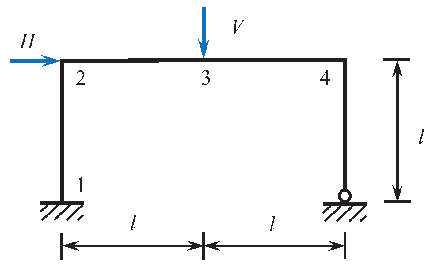
This example applies ALRMs to a rigid-plastic portal frame with four collapse modes [50,51]. As shown in Figure 4, this elastic–plastic structure is subjected to vertical and horizontal loads. Its performance function is defined as

$$G\left(\mathbf{x}\right)=min\left\{\begin{array}{c}{G}_1\hfill \\ G_2\hfill \\ G_3\hfill \\ G_4\hfill \end{array}\right\}=min\left\{\begin{array}{c}{M}_1+2M_3+2M_4-H-V\\ M_2+2M_3+M_4-V\\ M_1+M_2+M_4-H\\ M_1+2M_2+2M_3-H+V\end{array}\right\},$$

(18)

where $M_i$$(i=1,2,3,4)$ denotes the bearing capacity of node i; H and V represent the applied horizontal and vertical load, respectively. All plastic moment resistances and the external loads are assumed to follow independent normal distributions, with their means and standard deviations listed in

Table 3. Statistical properties of the rigid frame for Example 3.

Variable	${\mathit{M}}_1$	${\mathit{M}}_2$	${\mathit{M}}_3$	${\mathit{M}}_4$	H	V
Mean	1	1	1	1	1.05	1.5
Standard deviation	0.15	0.15	0.15	0.15	0.1785	0.75

. It should be noted that all random variables in this example are dimensionless quantities.

Table 4. Comparisons of results for Example 3.

Method	MCS	AK-MCS	ASVM-MCS	Proposed Method: ASVR-MCS
				$\mathit{L}$	${\mathit{\psi }}_{\mathrm{m}}$	$\mathit{P}$
${\widehat{P}}_f$	$3.339\times {10}^{-3}$	$3.125\times {10}^{-3}$	$3.268\times {10}^{-3}$	$3.358\times {10}^{-3}$	$3.299\times {10}^{-3}$	$3.267\times {10}^{-3}$
$N_{\mathrm{call}}$	$1.0\times {10}^6$	138.6	154.8	96.7	100.8	89.9
$\mathrm{Cov}\left({\widehat{P}}_f\right)$	-	27.76%	5.02%	4.9%	4.5%	3.55%
${\epsilon }_{\mathrm{r}}$	-	−6.4%	−2.1%	0.6%	−1.2%	−2.2%

summarizes the results for Example 3. The ${\widehat{P}}_f$ values estimated by all ALRMs are consistent with those from crude MCS. However, AK-MCS produces unstable estimates: it has a maximum coefficient of variation of 27.76% and a maximum relative error of −6.4%. Further analysis reveals that in 2 out of 30 repeated runs, the active learning process of AK-MCS terminated prematurely due to the convergence criterion. This suggests that the convergence criterion is overly relaxed for AK-MCS, resulting in a less accurate metamodel. ASVM-MCS requires more LSF calls but yields accurate results. In contrast, ASVR-MCS demonstrates robustness across all three learning functions, providing accurate ${\widehat{P}}_f$ estimates with the fewest LSF calls. Notably, ASVR-MCS+P requires the fewest LSF calls to meet the termination criteria and achieves the lowest coefficient of variation.

Figure 5 illustrates the convergence trend of ${\widehat{P}}_f$ with respect to the number of LSF calls (based on a typical run of each ALRM). ASVR-MCS+P begins to converge at approximately 40 calls, faster than ASVM-MCS (roughly 80 calls). AK-MCS appears to terminate at 60 calls, yielding an accurate approximate solution for this reliability problem. However, AK-MCS starts to diverge at 70 calls and exhibits unpredictable fluctuations at 110. This confirms that the active learning process of AK-MCS is insufficiently stable to produce reliable results.

3.4. Example Four

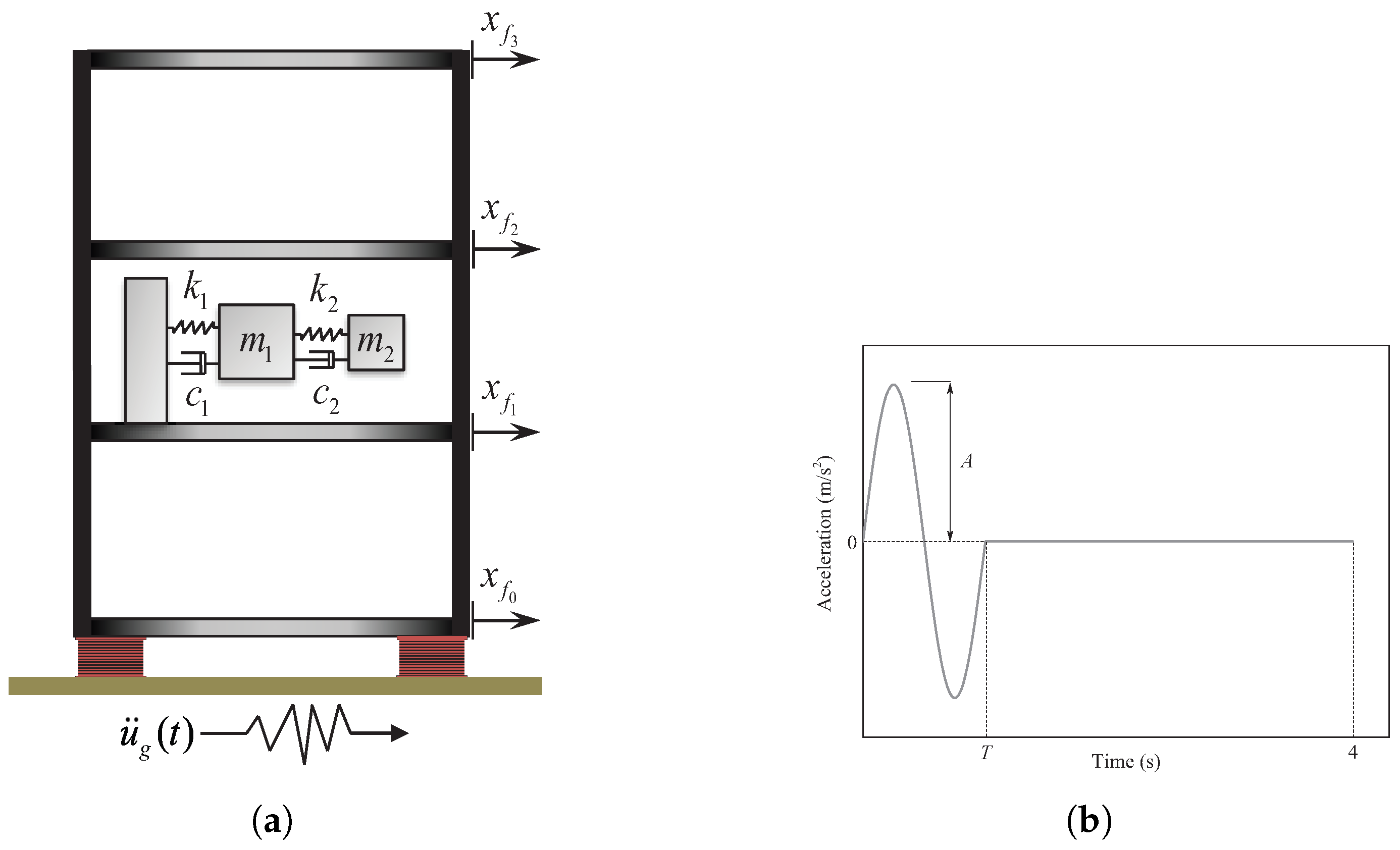
This example applies ALRMs to a dynamic isolation structure, considering comprehensive failures of the structure itself, the isolation layer, and the equipment [52,53]. Figure 6 shows the isolated structure and the applied ground acceleration excitation. An equipment isolation system is installed on the second floor, consisting of two degrees of freedom: one representing the isolation device with a mass of $m_1$ (500 kg) and the other representing shock-sensitive equipment with a mass of $m_2$ (100 kg). The corresponding spring stiffness and damper coefficients for these two degrees of freedom are illustrated in Figure 6, where $k_1$, $k_2$, $c_1$, and $c_2$ are equal to 2500 N/m, 105 N/m, 350 N/(m/s), and 200 N/(m/s), respectively. For simplicity, the motion of the lowest floor is resisted by an elastic isolation bearing. The bearing stiffness is determined by dividing the maximum horizontal force $F_y$ by the maximum horizontal displacement $D_y$. To reduce the number of variables, each floor is assumed to have the same mass ($m_f$), stiffness ($k_f$), and damping ($c_f$). The excitation is defined as a single-period sinusoidal impulse with period T and amplitude A. This problem involves seven independent random variables, all assumed to follow lognormal distributions. Their statistical parameters are given in

Table 5. The statistical properties of the random variables for Example 4.

Variable	Mean	Standard Deviation	Units
$m_f$	$6.00\times {10}^3$	$6.00\times {10}^2$	kg
$k_f$	$3.00\times {10}^7$	$3.00\times {10}^6$	N/m
$c_f$	$6.00\times {10}^4$	$1.20\times {10}^4$	N/(m/s)
$F_y$	$2.00\times {10}^4$	$4.00\times {10}^3$	N
$D_y$	$5.00\times {10}^{-2}$	$1.00\times {10}^{-2}$	m
T	1	$0.2$	s
A	1	$0.5$	${\mathrm{m}/\mathrm{s}}^2$

. The limit state function, defined by the combination of three failure modes, is expressed as

$$\begin{array}{cc}\hfill G\left(\mathbf{x}\right)& =12.50{(0.04-\underset{t}{max}\left|x_{f_i}\left(t\right)-x_{f_{i-1}}\left(t\right)\right|)}_{i=2,3,4}\hfill \\ \hfill & +(0.50-\underset{t}{max}\left|{\ddot{u}}_g\left(t\right)-{\ddot{x}}_{m_2}\left(t\right)\right|)\hfill \\ \hfill & +2.0(0.25-\underset{t}{max}\left|x_{f_2}\left(t\right)-x_{m_1}\left(t\right)\right|)\hfill \end{array},$$

(19)

where $x_{f_i}\left(t\right)$ is the displacement of the $i^{\mathrm{th}}$ floor; $x_{m_i}$ is the displacement of the mass block $m_i$ on the second floor; and ${\ddot{u}}_g\left(t\right)$ is the ground acceleration. The LSF in Equation (19) is a composite expression of three failure modes: the first term relates to the limit on interstory displacement, with a threshold of 0.04 m; the second term indicates that damage to the equipment will occur if its peak absolute acceleration exceeds 0.5 $\mathrm{m}/{\mathrm{s}}^2$; and the last term describes damage to the equipment isolator resulting from excessive displacement (threshold: 0.25 m). Each term is multiplied by weighting factors to emphasize the equal contribution of the three individual failure modes [52].

Considering computational time limitations, the maximum number of calls to the true performance function is set to 200 in this example. In

Table 6. Comparisons of results for Example 4.

Method	MCS	AK-MCS	ASVM-MCS	Proposed Method: ASVR-MCS
				$\mathit{L}$	${\mathit{\psi }}_{\mathrm{m}}$	$\mathit{P}$
${\widehat{P}}_f$	$4.654\times {10}^{-2}$	$4.632\times {10}^{-2}$	$8.782\times {10}^{-2}$	$4.616\times {10}^{-2}$	$4.646\times {10}^{-2}$	$4.619\times {10}^{-2}$
$N_{\mathrm{call}}$	$1.0\times {10}^6$	106.6	105.1	52.2	51.2	56.9
$\mathrm{Cov}\left({\widehat{P}}_f\right)$	-	3.51%	166.23%	2.54%	1.63%	2.46%
${\epsilon }_{\mathrm{r}}$	-	−0.5%	88.7%	−0.8%	−0.2%	−0.8%

, the proposed ASVR-MCS method is compared with the crude MCS and other ALRMs. It is observed that ASVR-MCS—using three different learning functions—yields accurate ${\widehat{P}}_f$ values and requires the lowest number of calls to the performance function. Furthermore, the ${\widehat{P}}_f$ value calculated by AK-MCS is identical to the reference value; however, AK-MCS requires nearly twice as many calls to the performance function as ASVR-MCS. Meanwhile, AK-MCS exhibits lower accuracy in terms of $\mathrm{Cov}\left({\widehat{P}}_f\right)$, which is slightly higher than that of ASVR-MCS. Nevertheless, ASVM-MCS yields the least accurate results, with a maximum $\mathrm{Cov}\left({\widehat{P}}_f\right)$ of 166.23% and a maximum relative error of 88.7%.

The evolution of the failure probability with respect to the number of training samples is plotted in Figure 7. ASVR-MCS (Figure 7c) converges to the “exact” solution with only 40 calls to the performance function, whereas AK-MCS (Figure 7a) requires at least 80 samples to obtain steady and accurate results. It is evident that ASVM-MCS (Figure 7b) fails to converge to the reference value. Therefore, the proposed ASVR-MCS method outperforms all other methods, demonstrating the highest efficiency and accuracy.

4. Conclusions

Methods that combine an adaptive metamodel with a numerical simulation method are efficient and hold promise for solving structural reliability problems involving time-demanding numerical models. Based on the framework of AK-MCS [5], this paper proposed a novel active learning reliability method—termed ASVR-MCS—which integrates adaptive support vector regression with Monte Carlo simulation. The active learning strategy has been modified to further enhance efficiency and accuracy. Two existing learning functions (L and ${\psi }_{\mathrm{m}}$) and one novel learning function (P, based on the penalty function method) are introduced to identify optimal points at each iteration. Four examples of structural reliability problems—featuring multiple failure points, disjoint failure regions, or implicit LSFs—were investigated. The applicability, efficiency, and accuracy of the proposed method were compared with those of two other ALRMs: AK-MCS and ASVM-MCS.

Based on the numerical results, the three ALRMs each exhibit distinct merits depending on the features of the performance function. Specifically, AK-MCS excels at modeling performance functions with continuous nonlinearity; however, it may become intractable when addressing discontinuity issues, particularly infinite discontinuities. Conversely, ASVM-MCS is more suitable for addressing infinite discontinuity problems but consistently performs poorly when dealing with problems involving multiple failure regions. In contrast, ASVR-MCS provides an excellent solution for problems with discontinuous derivatives and demonstrates favorable computational efficiency and accuracy when addressing problems involving infinite discontinuities or multiple failure regions. Furthermore, all three learning functions (L, ${\psi }_{\mathrm{m}}$, and P) employed in the proposed ASVR-MCS method yield accurate results, which are nearly identical to those obtained via crude MCS. Similar levels of efficiency—measured by the number of calls to the LSF—are achieved when using the three different learning functions; however, the proposed function P is preferable due to its more accurate estimation of the failure probability. It should be noted that ASVR-MCS is mainly applicable to low- to moderate-dimensional problems. Further investigation is needed to extend its application to high-dimensional problems. While the simplification of the numerical examples regarding the factors such as material uncertainties and variable correlations facilitates clear validation against established problems and highlights the core methodology’s potential, it inevitably limits direct applicability to real-world engineering scenarios. Extending the framework to handle stochastic material properties and variable correlations constitutes an important direction for our subsequent research.

References

1. Zheng, Z.; Dai, H.; Beer, M. Efficient structural reliability analysis via a weak-intrusive stochastic finite element method. Probabilistic Eng. Mech. 2023, 71, 103414. [Google Scholar] [CrossRef]
2. Wang, B.; Ma, S.; Li, Y.P.; Wang, N.; Ren, Q.X. Axial compression mechanical properties of UHTCC-hollow steel tube square composited short columns. J. Constr. Steel Res. 2025, 228, 109424. [Google Scholar] [CrossRef]
3. Proppe, C. Estimation of failure probabilities by local approximation of the limit state function. Struct. Saf. 2008, 30, 277–290. [Google Scholar] [CrossRef]
4. Zhang, R.; Dai, H. Stochastic analysis of structures under limited observations using kernel density estimation and arbitrary polynomial chaos expansion. Comput. Methods Appl. Mech. Eng. 2023, 403, 115689. [Google Scholar] [CrossRef]
5. Echard, B.; Gayton, N.; Lemaire, M. AK-MCS: An active learning reliability method combining Kriging and Monte Carlo Simulation. Struct. Saf. 2011, 33, 145–154. [Google Scholar] [CrossRef]
6. Dai, H.; Zhang, R.; Beer, M. A new method for stochastic analysis of structures under limited observations. Mech. Syst. Signal Process. 2023, 185, 109730. [Google Scholar] [CrossRef]
7. Fauriat, W.; Gayton, N. AK-SYS: An adaptation of the AK-MCS method for system reliability. Reliab. Eng. Syst. Saf. 2014, 123, 137–144. [Google Scholar] [CrossRef]
8. Dai, H.; Zhang, R.; Beer, M. A new perspective on the simulation of cross-correlated random fields. Struct. Saf. 2022, 96, 102201. [Google Scholar] [CrossRef]
9. Zhang, R.; Dai, H. A non-Gaussian stochastic model from limited observations using polynomial chaos and fractional moments. Reliab. Eng. Syst. Saf. 2022, 221, 108323. [Google Scholar] [CrossRef]
10. Wang, B.; Zhang, Y.J.; Ren, Q.X.; Feng, H.Y.; Bi, R.; Zhao, X. Axial compression properties of reinforced concrete columns strengthened with textile-reinforced ultra-high toughness cementitious composite in chloride environment. J. Build. Eng. 2025, 111, 113116. [Google Scholar] [CrossRef]
11. Wang, M.; Zhang, H.; Dai, H.; Shen, L. A deep learning-aided seismic fragility analysis method for bridges. Structures 2022, 40, 1056–1064. [Google Scholar] [CrossRef]
12. Dai, H.; Zhang, R.; Zhang, H. A new fractional moment equation method for the response prediction of nonlinear stochastic systems. Nonlinear Dyn. 2019, 97, 2219–2230. [Google Scholar] [CrossRef]
13. Blatman, G.; Sudret, B. Adaptive sparse polynomial chaos expansion based on least angle regression. J. Comput. Phys. 2011, 230, 2345–2367. [Google Scholar] [CrossRef]
14. Zhang, R.; Dai, H. An optimal transport method for the PC representation of non-Gaussian fields. Mech. Syst. Signal Process. 2025, 224, 112172. [Google Scholar] [CrossRef]
15. Cadini, F.; Santos, F.; Zio, E. An improved adaptive kriging-based importance technique for sampling multiple failure regions of low probability. Reliab. Eng. Syst. Saf. 2014, 131, 109–117. [Google Scholar] [CrossRef]
16. Echard, B.; Gayton, N.; Lemaire, M.; Relun, N. A combined Importance Sampling and Kriging reliability method for small failure probabilities with time-demanding numerical models. Reliab. Eng. Syst. Saf. 2013, 111, 232–240. [Google Scholar] [CrossRef]
17. Bichon, B.J.; Eldred, M.S.; Swiler, L.P.; Mahadevan, S.; McFarland, J.M. Efficient Global Reliability Analysis for Nonlinear Implicit Performance Functions. AIAA J. 2008, 46, 2459–2468. [Google Scholar] [CrossRef]
18. Papadopoulos, V.; Giovanis, D.G.; Lagaros, N.D.; Papadrakakis, M. Accelerated subset simulation with neural networks for reliability analysis. Comput. Methods Appl. Mech. Eng. 2012, 223–224, 70–80. [Google Scholar] [CrossRef]
19. Xiao, N.C.; Zuo, M.J.; Zhou, C. A new adaptive sequential sampling method to construct surrogate models for efficient reliability analysis. Reliab. Eng. Syst. Saf. 2018, 169, 330–338. [Google Scholar] [CrossRef]
20. Pan, Q.; Dias, D. An efficient reliability method combining adaptive Support Vector Machine and Monte Carlo Simulation. Struct. Saf. 2017, 67, 85–95. [Google Scholar] [CrossRef]
21. Bourinet, J.M.; Deheeger, F.; Lemaire, M. Assessing small failure probabilities by combined subset simulation and Support Vector Machines. Struct. Saf. 2011, 33, 343–353. [Google Scholar] [CrossRef]
22. Basudhar, A.; Missoum, S. Adaptive explicit decision functions for probabilistic design and optimization using support vector machines. Comput. Struct. 2008, 86, 1904–1917. [Google Scholar] [CrossRef]
23. Basudhar, A.; Missoum, S. An improved adaptive sampling scheme for the construction of explicit boundaries. Struct. Multidiscip. Optim. 2010, 42, 517–529. [Google Scholar] [CrossRef]
24. Hurtado, J.E. Filtered importance sampling with support vector margin: A powerful method for structural reliability analysis. Struct. Saf. 2007, 29, 2–15. [Google Scholar] [CrossRef]
25. Gaspar, B.; Teixeira, A.; Soares, C.G. Assessment of the efficiency of Kriging surrogate models for structural reliability analysis. Probabilistic Eng. Mech. 2014, 37, 24–34. [Google Scholar] [CrossRef]
26. Bourinet, J.M. Rare-event probability estimation with adaptive support vector regression surrogates. Reliab. Eng. Syst. Saf. 2016, 150, 210–221. [Google Scholar] [CrossRef]
27. Roy, A.; Chakraborty, S. Support vector regression based metamodel by sequential adaptive sampling for reliability analysis of structures. Reliab. Eng. Syst. Saf. 2020, 200, 106948. [Google Scholar] [CrossRef]
28. Sun, Z.; Wang, J.; Li, R.; Tong, C. LIF: A new Kriging based learning function and its application to structural reliability analysis. Reliab. Eng. Syst. Saf. 2017, 157, 152–165. [Google Scholar] [CrossRef]
29. Huang, X.; Chen, J.; Zhu, H. Assessing small failure probabilities by AK–SS: An active learning method combining Kriging and Subset Simulation. Struct. Saf. 2016, 59, 86–95. [Google Scholar] [CrossRef]
30. Guo, Q.; Liu, Y.; Chen, B.; Zhao, Y. An active learning Kriging model combined with directional importance sampling method for efficient reliability analysis. Probabilistic Eng. Mech. 2020, 60, 103054. [Google Scholar] [CrossRef]
31. Ling, C.; Lu, Z.; Cheng, K.; Sun, B. An efficient method for estimating global reliability sensitivity indices. Probabilistic Eng. Mech. 2019, 56, 35–49. [Google Scholar] [CrossRef]
32. Qian, J.; Yi, J.; Cheng, Y.; Liu, J.; Zhou, Q. A sequential constraints updating approach for Kriging surrogate model-assisted engineering optimization design problem. Eng. Comput. 2019, 36, 993–1009. [Google Scholar] [CrossRef]
33. Wang, Z.; Broccardo, M. A novel active learning-based Gaussian process metamodelling strategy for estimating the full probability distribution in forward UQ analysis. Struct. Saf. 2020, 84, 101937. [Google Scholar] [CrossRef]
34. Ren, C.; Aoues, Y.; Lemosse, D.; Souza De Cursi, E. Ensemble of surrogates combining Kriging and Artificial Neural Networks for reliability analysis with local goodness measurement. Struct. Saf. 2022, 96, 102186. [Google Scholar] [CrossRef]
35. Moustapha, M.; Marelli, S.; Sudret, B. Active learning for structural reliability: Survey, general framework and benchmark. Struct. Saf. 2022, 96, 102174. [Google Scholar] [CrossRef]
36. Zhang, R.; Dai, H. Independent component analysis-based arbitrary polynomial chaos method for stochastic analysis of structures under limited observations. Mech. Syst. Signal Process. 2022, 173, 109026. [Google Scholar] [CrossRef]
37. Shi, L.; Sun, B.; Ibrahim, D.S. An active learning reliability method with multiple kernel functions based on radial basis function. Struct. Multidiscip. Optim. 2019, 60, 211–229. [Google Scholar] [CrossRef]
38. Wang, J.; Li, C.; Xu, G.; Li, Y.; Kareem, A. Efficient structural reliability analysis based on adaptive Bayesian support vector regression. Comput. Methods Appl. Mech. Eng. 2021, 387, 114172. [Google Scholar] [CrossRef]
39. Zhou, T.; Peng, Y. An active-learning reliability method based on support vector regression and cross validation. Comput. Struct. 2023, 276, 106943. [Google Scholar] [CrossRef]
40. Vapnik, V.N. The Nature of Statistical Learning Theory, 2nd ed.; Springer: New York, NY, USA, 1995. [Google Scholar] [CrossRef]
41. Dai, H.; Li, D.; Beer, M. Adaptive Kriging-assisted multi-fidelity subset simulation for reliability analysis. Comput. Methods Appl. Mech. Eng. 2025, 436, 117705. [Google Scholar] [CrossRef]
42. Thapa, A.; Roy, A.; Chakraborty, S. Reliability analyses of underground tunnels by an adaptive support vector regression model. Comput. Geotech. 2024, 172, 106418. [Google Scholar] [CrossRef]
43. Asgarkhani, N.; Kazemi, F.; Jankowski, R. Machine-learning based tool for seismic response assessment of steel structures including masonry infill walls and soil-foundation-structure interaction. Comput. Struct. 2025, 317, 107918. [Google Scholar] [CrossRef]
44. Baidya, S.; Roy, B.K. Seismic reliability analysis of base isolated building supplemented with shape memory alloy rubber bearing using support vector regression metamodel. Structures 2024, 65, 106773. [Google Scholar] [CrossRef]
45. Moustapha, M.; Lataniotis, C.; Wiederkehr, P.; Wicaksono, D.; Marelli, S.; Sudret, B. UQLib User Manual; Technical Report; Chair of Risk, Safety & Uncertainty Quantification, ETH Zurich: Zürich, Switzerland, 2019; Report # UQLab-V1.2-201. [Google Scholar]
46. Xue, G.; Lyu, X. An Adaptive Clustering-Based Active Learning Kriging Method Combining with Importance Sampling for Structural Reliability Analysis with Multiple Failure Regions. IEEE Access 2025, 13, 150308–150320. [Google Scholar] [CrossRef]
47. Su, M.; Xue, G.; Wang, D.; Zhang, Y.; Zhu, Y. A novel active learning reliability method combining adaptive Kriging and spherical decomposition-MCS (AK-SDMCS) for small failure probabilities. Struct. Multidiscip. Optim. 2020, 62, 3165–3187. [Google Scholar] [CrossRef]
48. Robert, C.; Casella, G. Monte Carlo Statistical Methods, 2nd ed.; Springer Science & Business Media: New York, NY, USA, 2004. [Google Scholar]
49. Katsuki, S.; Frangopol, D.M. Hyperspace Division Method for Structural Reliability. J. Eng. Mech. 1994, 120, 2405–2427. [Google Scholar] [CrossRef]
50. Melchers, R.E. Radial Importance Sampling for Structural Reliability. J. Eng. Mech. 1990, 116, 189–203. [Google Scholar] [CrossRef]
51. Cui, F.; Ghosn, M. Implementation of machine learning techniques into the Subset Simulation method. Struct. Saf. 2019, 79, 12–25. [Google Scholar] [CrossRef]
52. Dai, H.; Cao, Z. A Wavelet Support Vector Machine-Based Neural Network Metamodel for Structural Reliability Assessment. Comput.-Aided Civ. Infrastruct. Eng. 2017, 32, 344–357. [Google Scholar] [CrossRef]
53. Gavin, H.P.; Yau, S.C. High-order limit state functions in the response surface method for structural reliability analysis. Struct. Saf. 2008, 30, 162–179. [Google Scholar] [CrossRef]
Figure 1. Comparison of predicted LSF (red dotted lines) and true LSF (green lines), along with DoE distribution (light blue squares = initial DoE; dark blue crosses = DoE after enrichment) for Example 1. The total number of DoE samples for each algorithm in this typical run is 41 (AK-MCS), 93 (ASVM-MCS), and 54 (ASVR-MCS+P).
Buildings 15 04183 g001
Figure 2. Comparison of added best points (dark blue crosses) and initial DoE samples (light blue circles) for ASVR-MCS using different learning functions for Example 1. Red dotted lines = predicted LSF; green lines = true LSF.
Buildings 15 04183 g002
Figure 3. A three-dimensional plot of the performance function for Example 2.
Buildings 15 04183 g003
Figure 4. Rigid frame of Example 3. The numbers 1 through 4 indicate the node labels.
Buildings 15 04183 g004
Figure 5. Convergence trend of P ^ f versus the number of calls to LSF for Example 3. The horizontal red dotted line indicates the reference failure probability calculated by MCS.
Buildings 15 04183 g005
Figure 6. Isolation system of Example 4: (a) Base-isolated structure with an equipment isolation system on the second floor; (b) Acceleration history of a single-period sinusoidal impulse.
Buildings 15 04183 g006
Figure 7. Convergence trend of P ^ f versus the number of calls to LSF for Example 4. The horizontal red dotted line indicates the reference failure probability calculated by MCS.
Buildings 15 04183 g007