Prediction of Concrete Abrasion Depth in Hydraulic Structures Using an Interpretable Hybrid Ensemble Model Based on Meta-Heuristic Algorithms

Abstract

The concrete protective layer in hydraulic tunnels is prone to abrasion by high-velocity sand-laden water, reducing structural durability. Accurate prediction of abrasion depth is key to rational hydraulic structure design. Existing studies have limitations: classical empirical models consider only a single factor, while early machine learning models fail to cover two core abrasion mechanisms (friction and impact) and lack meta-heuristic algorithm-based parameter optimization, leading to insufficient generalization and stability. This study aims to (1) establish a multi-source database with 690 cases (463 friction-dominated, 227 impact-dominated) covering multiple test standards (ASTM C944, ASTM C779, BIS: 1237-1980, ASTM C1138); (2) optimize hyperparameters of LightGBM, XGBoost, and CatBoost using Genghis Khan Shark Optimizer (GKSO) to build a hybrid ensemble model; (3) verify model performance and identify key factors via SHAP analysis. After preprocessing, input features were simplified to five: water–cement ratio, FA/CA (fine aggregate/coarse aggregate), age, T/V (test duration/velocity), and WRA content. Results show that GKSO-CatBoost performed best (test set R² = 0.982, RMSE = 0.1231 mm). SHAP analysis identified T/V and the water–cement ratio as key influencing features, providing clear directions for optimizing concrete mix proportions under different standard scenarios. This study provides a new method for hydraulic concrete abrasion prediction and a scientific basis for durability design oriented to specific test standards.

1. Introduction

Concrete is widely used in various industries as one of the main materials for structures. Therefore, it is expected that concrete should possess certain minimum durability, particularly in terms of strength, impact resistance, permeability, freeze–thaw resistance, and abrasion resistance [1]. During the service life of hydraulic tunnel concrete, it undergoes severe abrasion damage due to hydraulic conditions, such as the impact of high-velocity sand-laden water and its own performance factors. Studying concrete abrasion damage is a complex issue, and the lack of a convenient and accurate abrasion depth prediction model has brought many difficulties to the durability design of hydraulic tunnels.

The abrasion resistance of concrete is influenced by multiple factors, including concrete mix proportion, curing age, and hydraulic conditions. To investigate these influencing factors, scholars have conducted targeted experiments: Ghafoori et al. [2] performed tests in accordance with ASTM C 779 [3] Procedure C and found that the water–cement ratio (0.21–0.34) and aggregate–cement ratio (9:1–3:1) exerted significant effects. When the 28-day standard-cured concrete achieved a compressive strength of 40–79 MPa, its abrasion resistance improved with optimized mix proportions. Siddique et al. [4] replaced fine aggregates with 35–55% Class F fly ash and confirmed that this admixture could significantly enhance the full-age abrasion resistance of concrete. Ghafoori and Diawara [5] discovered that replacing 5–20% of fine aggregates with silica fume improved abrasion resistance, and the improvement effect continued to strengthen until the silica fume content reached 10%. Zhu et al. [6] combined the underwater methods specified in ASTM C1138 [7] and SL 352-2006 [8], and clarified that the coupling of freeze–thaw cycles and hydraulic abrasion exacerbates concrete abrasion depth. From the aforementioned literature, it is evident that concrete abrasion resistance is not determined by a single factor, but rather a core property jointly regulated by material mix proportion, curing conditions, environmental factors, and hydraulic actions.

In the field of concrete abrasion depth prediction, early scholars conducted extensive research on empirical and semi-empirical models, laying a foundation for subsequent studies. However, limited by their modeling approaches, these models still have significant shortcomings and cannot meet the demands of practical engineering [9].

For classical empirical models, researchers constructed prediction models by focusing on the correlation between a single factor and abrasion depth, resulting in typical forms such as linear, polynomial, and power function models. Among them, Naik et al. [10] conducted abrasion tests using the rotating cutter method in accordance with ASTM C-944 [11] and pointed out that within a certain compressive strength range, the abrasion depth of concrete is inversely proportional to its compressive strength, thereby establishing a quantitative correlation between mechanical properties and abrasion damage. Horszczaruk [12] studied high-strength concrete for hydraulic structures based on the ASTM C 1138 [7] method and proposed a polynomial model between abrasion depth and compressive strength, filling the gap in abrasion prediction for high-strength concrete.

Siddique et al. [4] used a power function in the form of y = ax^−b to fit the relationships between abrasion depth and multiple mechanical indicators (e.g., compressive strength, splitting tensile strength), increasing the model’s goodness of fit R² to over 0.93. Zhu et al. [6] also employed a power function to develop an abrasion depth prediction model under different freeze–thaw cycles, incorporating environmental factors into the empirical prediction framework. Nevertheless, the limitations of such models are equally prominent: the models by Naik and Horszczaruk can only characterize the single relationship between abrasion depth and compressive strength, failing to reflect the coupling effects of other key factors, such as mix proportion and hydraulic conditions. Even though the models by Siddique and Zhu expanded the coverage of influencing factors, they still suffer from narrow applicability—the former is only suitable for specific mechanical property test conditions, while the latter is limited to freeze–thaw coupling environments. Therefore, these models are difficult to apply to complex abrasion scenarios in practical engineering, and their overall prediction accuracy is constrained by the single-factor modeling approach, which cannot meet the requirements of high-precision design.

In the field of semi-empirical models, Bitter et al. [13,14,15] developed semi-empirical models by combining experimental measurements and mathematical theory, thereby improving prediction accuracy. However, the application of these semi-empirical models is limited to specific operating ranges or specially designed experiments [16]; once outside this scope, the prediction deviation of the models increases significantly, making it difficult to achieve engineering-level generalization.

With the development of artificial intelligence technology, machine learning (ML) methods, relying on their strong capabilities in multi-feature information processing and complex relationship learning, have gradually replaced traditional empirical models and become a research hotspot in concrete abrasion depth prediction. Compared with empirical models that can only fit a single factor, algorithms such as artificial neural networks (ANNs), random forests (RFs), and Extreme Gradient Boosting (XGBoost) can integrate multi-dimensional parameters (e.g., concrete properties, hydraulic conditions), significantly enhancing prediction flexibility. For example, Gencel et al. [1] correlated factors such as metal aggregate content, cement content, and applied load using an ANN model, confirming that its prediction accuracy was significantly superior to that of the traditional general linear model (GLM), and verifying the advantages of ML methods in multi-variable abrasion prediction for the first time. Liu [16] further integrated three core factors (hydraulic conditions, curing age, and concrete mix proportion), and constructed a model by combining Bayesian optimization with the RF-ANN algorithm, overcoming the limitation of “incomplete feature coverage” in early ML models. Based on Liu’s dataset, Moghaddas [17] optimized the hyperparameters of five different ML algorithms using the Parsen Tree Estimator (PTE) [18] for prediction, while Amin [19] used multi-expression programming (MEP) and gene expression programming (GEP) for prediction, further promoting the accuracy improvement of ML models.

However, existing ML studies still have gaps that prevent them from being directly applied to the complex engineering needs of hydraulic structures. First, incomplete data coverage and abrasion mechanism characterization. Malazdrewicz [20] and Sadowski [21] and others built models based on small-sample data from the single ASTM C944 standard [11], which only simulates dry friction scenarios and cannot cover the actual “friction–impact coexistence” abrasion mechanism of hydraulic tunnels (as shown in Figure 1, the normal force caused by impact and the shear force caused by friction jointly exacerbate abrasion, and these two effects are difficult to manifest simultaneously in a single standard test). Second, limitations in hyperparameter optimization methods and model architecture. Existing studies mostly use Bayesian optimization (Liu [16]), PTE (Moghaddas [17]) or evolutionary algorithms (Amin [19]) to optimize single ML models and have not yet combined meta-heuristic algorithms with EL (ensemble learning). Ensemble learning significantly improves the accuracy of models in prediction tasks and their robustness against data disturbances; compared with single ML models, EL more effectively handles data noise and bias, reduces the risk of overfitting, and exhibits stronger robustness and generalization ability in complex problems [22]. Recent studies have further shown that ensemble models combined with meta-heuristic algorithms outperform traditional ensemble models [23].

As an advancement of heuristic algorithms (which generate a fixed output for a given input), meta-heuristic algorithms are non-deterministic methods due to the inclusion of random factors [24]. A meta-heuristic algorithm is a problem-independent technique that does not leverage any specific characteristics of the target problem. It is a combination of random algorithms and local search algorithms. This type of non-deterministic method uses randomly generated variables to explore near-optimal solutions within the problem space [25]. Meta-heuristic algorithms are often employed to optimize model hyperparameters, thereby enhancing model robustness. The Genghis Khan Shark Optimizer (GKSO), proposed in 2023, exhibits advantages such as strong optimization capability, advanced search strategies, and low parameter sensitivity.

Therefore, this study developed three hybrid ensemble models based on GKSO and ensemble learning to predict the abrasion depth of concrete used in hydraulic tunnels. By integrating multi-standard test data and introducing SHAP (SHapley Additive exPlanations) feature analysis, the models can not only adapt to the dual mechanisms of friction and impact but also provide quantitative basis for engineering design—rather than merely focusing on improving theoretical accuracy.

Based on this, the innovation of this study is specifically reflected in the following three aspects:

(1)

Combining the meta-heuristic algorithm (GKSO) with three mainstream ensemble algorithms (LightGBM, XGBoost, and CatBoost). GKSO is used for efficient hyperparameter optimization, and 5-fold cross-validation is adopted to enhance generalization ability.

(2)

Achieving high-precision prediction for datasets under two abrasion mechanisms (friction and impact). Through additional feasibility validation tests to verify the reliability of the model.

(3)

Introducing SHAP analysis to quantify the influence weight of each feature, identifying the T/V ratio (ratio of abrasion test time to loading speed) and water–cement ratio as key influencing factors. This transforms the “black-box” model into an interpretable decision-making tool, providing clear parameter adjustment directions for the optimization of concrete mix proportion.

2. Methods

2.1. Data Collection

Developing a highly representative and comprehensive database is a key prerequisite for ensuring sufficient model training and reliable validation. Based on a systematic review and knowledge extraction from the existing literature, this study established a comprehensive database covering a wide range of information dimensions, including experimental data under various standard tests.

Table 1. Data classification and sources.

Abrasion Type	Method	Number of Data	Concrete Mix Parameters (kg/m3)	Data Source
Friction	ASTM C944	216	Cement: 259–398	[28]
			Fly ash: 0–139
			Silica fume: 0
			Steel fiber: 0
			Fine aggregate: 677–715
			Coarse aggregate: 1172–1164
			Water: 123–139
			WRA: 2.7–2.9
	ASTM C779	79	Cement: 110–564	[10,29,30,31]
			Fly ash: 0–316
			Silica fume: 0–54
			Steel fiber: 0–60
			Fine aggregate: 606–1005
			Coarse aggregate: 735–1182
			Water: 116–254
			WRA: 0–5.13
	BIS: 1237–1980	169	Cement: 235–470	[32,33]
			Fly ash: 0–235
			Silica fume: 0
			Steel fiber: 0
			Fine aggregate: 554–620
			Coarse aggregate: 916–1139
			Water: 129–208
			WRA: 1.98–2.87
Impact	ASTM C1138	227	Cement: 265–643	[6,12,30,34,35,36,37]
			Fly ash: 0–265
			Silica fume: 0–54
			Steel fiber: 0–70
			Fine aggregate: 425–1007
			Coarse aggregate: 743–1279
			Water: 116–220
			WRA: 0–17.86

provides detailed information. The ASTM C944 standard uses the rotating steel bristle method (load 445 N, rotation speed 70 rpm) to test concrete abrasion resistance. This method simulates dry contact abrasion mechanisms through continuous shearing action and quantifies the average abrasion depth after 500 rotations (accuracy 0.01 mm). The test results can be correlated to the floor of hydraulic spillways in actual engineering (sediment deposition friction when there is no water flow). The ASTM C779-20 [26] standard evaluates concrete abrasion resistance using a turntable-type composite abrasion test. A floating turntable simultaneously applies three grinding heads (steel wheel, cast iron knife, steel ball) and rotates 60 times under a normal load of 147 N, with abrasion depth converted from mass loss. The Indian Standard Specification BIS: 1237-1980 [27] method uses the rotating water–sand jet method to test concrete abrasion resistance. Quartz sand (particle size of 0.3–0.6 mm) is mixed with water at a mass ratio of 3:1 and impacts the surface of rotating specimens through a 45° inclined nozzle at a flow rate of 8 L/min for 60 min, with abrasion depth calculated from mass loss. This method is particularly suitable for abrasion assessment in hydraulic engineering with high sediment-laden rivers. The ASTM C1138 standard uses the rotating steel ball water-impact method to evaluate the hydraulic abrasion performance of concrete. A total of 100 steel balls with a diameter of 12.7 mm are driven by water flow at 1200 rpm to form vertical jumping impacts, and abrasion depth is measured by surface morphology scanning after 12 h of continuous action. This method accurately simulates the scouring effect of high-speed water flow on concrete through kinetic energy conversion mechanisms.

The established database includes the following input features: concrete mix components (cement, fly ash, silica fume, steel fiber, water, fine aggregate, coarse aggregate, WRA (water-reducing agent), age, time of testing, abrasion condition, and velocity). The main abrasion conditions are divided into friction and impact, which is a categorical variable encoded as 0 for friction and 1 for impact. The rotation speed in each standard was converted to linear velocity using the formula in Reference [16], in two steps as shown in Equations (3) and (4):

$$W_r={\displaystyle \frac{RPM}{60}}\cdot 2\pi$$

(1)

$$V_1=W_r\cdot R_a$$

(2)

where RPM is the rotation speed (rev/min), $W_r \mathrm{is} \mathrm{the} \mathrm{angular} \mathrm{velocity} \left({\displaystyle \frac{\mathrm{rad}}{\mathrm{s}}}\right), \mathrm{and} V_1$ is the linear velocity (m/s).

2.2. Feature Selection and Multicollinearity Analysis

Hughes effect proves that when the number of features exceeds the optimal threshold, model accuracy decreases exponentially with the increase in features [38]. The core cause of this phenomenon lies in the fact that excessive redundant or weakly correlated features introduce noise interference, increasing the model’s learning complexity. This significantly heightens the risk of overfitting to training data while obscuring the effective contribution of key features to prediction outcomes. Therefore, prior to constructing a concrete wear depth prediction model, the scientific screening and removal of redundant initial input features constitute a necessary preliminary step to safeguard model predictive performance and enhance model stability.

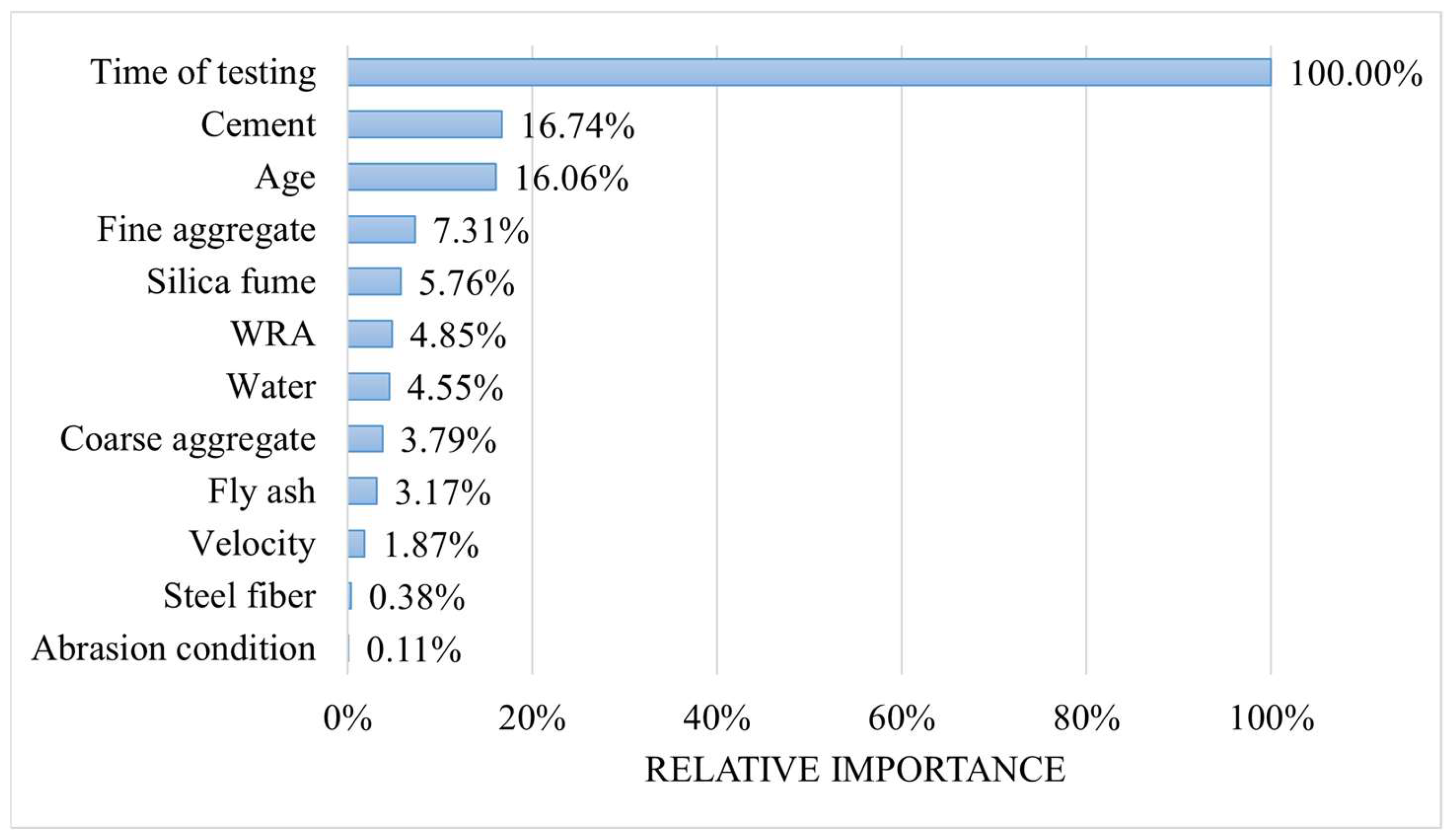
To achieve efficient feature screening, this study employs random forest (RF) technology within the Embedded Method for feature importance assessment. As an ensemble learning algorithm, random forest accomplishes classification or regression tasks by constructing multiple independent decision trees and synthesizing their predictions. Its core principle for feature importance evaluation relies on quantifying calculations based on node impurity reduction: During each decision tree’s construction, the algorithm traverses all candidate features, selecting the one that maximally reduces node impurity (typically the Gini coefficient for classification tasks or mean squared error for regression tasks) to perform node splitting. Upon completing training for each individual decision tree, the total impurity reduction contributed by that feature across all split nodes is calculated. The average of this metric across all trees in the forest is then derived, yielding the feature’s importance score. A higher score indicates greater contribution to reducing prediction error and enhancing decision accuracy, while a lower score suggests lower information content or potential redundancy. Figure 2 presents the results obtained using RF technology. The findings indicate that the primary wear conditions and steel fiber content exhibit extremely low significance values; consequently, both features are excluded.

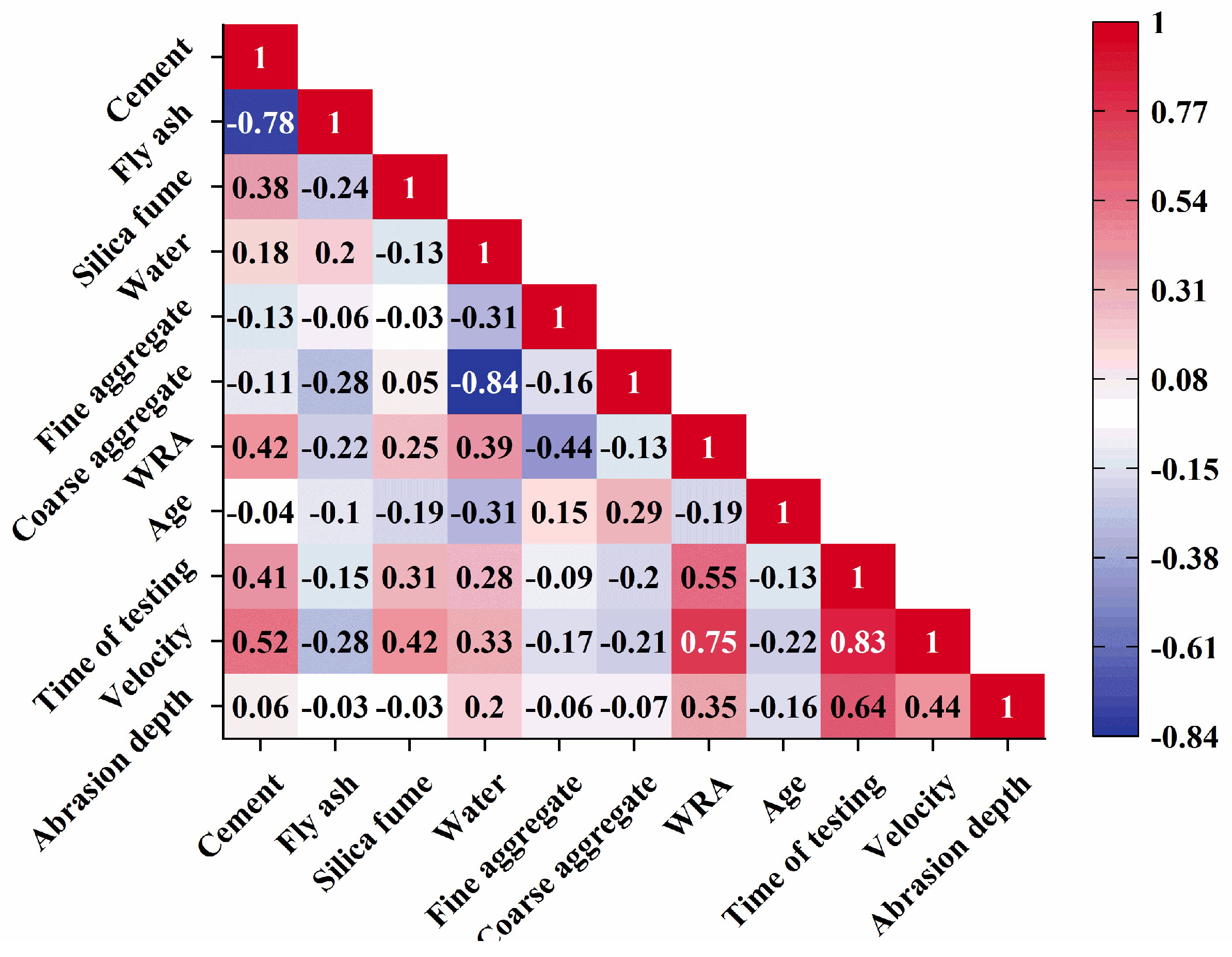
Multicollinearity refers to a high degree of correlation between independent variables in a dataset, which can significantly affect the accuracy of regression models [39]. To quantitatively assess the severity of multicollinearity within the initial dataset (detailed statistics are presented in

Table 2. Distribution statistics of database before feature reconstruction.

	MEAN	STD	MIN	MID	MAX
Cement (kg/m3)	378.91	97.18	110	397	643
Fly ash (kg/m3)	66.35	86.09	0	0	316
Silica fume (kg/m3)	5.67	16.59	0	0	70
Water (kg/m3)	170.60	36.12	116	185	254
Fine aggregate (kg/m3)	655.14	102.66	425	621	1007
Coarse aggregate (kg/m3)	1066.39	148.08	735	1096	1279
WRA (kg/m3)	5.01	4.21	0	2.90	17.86
Age (d)	88.86	112.83	7	28	365
Test duration (s)	67,447	111,079	300	2700	432,000
Velocity (m/s)	3.37	3.28	0.65	1.00	8.00
Ad (mm)	1.36	1.06	0.04	1.13	8.43

), this study employs a dual diagnostic approach utilizing both the Pearson correlation coefficient (R) and the variance inflation factor (VIF). The Pearson correlation coefficient measures the strength of linear association between two continuous variables, with a values range of [−1, 1]. A higher absolute value approaching 1 indicates stronger linear correlation between variables (absolute values ≥ 0.7 are typically considered indicative of strong multicollinearity), while values closer to 0 denote weaker linear relationships. By computing the Pearson correlation matrix between all pairs of independent variables, one can preliminarily identify feature combinations exhibiting high linear association. The variance inflation factor, however, further quantifies the impact of multicollinearity on regression coefficient variance by assessing the extent to which an independent variable is linearly influenced by others. The standard interpretation of VIF values is as follows: VIF = 1 indicates complete independence of the independent variable from others, with no multicollinearity; 1 < VIF < 10 signifies weak multicollinearity, with negligible impact on the model; VIF ≥ 10 indicates severe multicollinearity. Figure 3 displays the correlation coefficients R between features, revealing high correlations between fly ash and cement, water and coarse aggregate, velocity and WRA, as well as between velocity and test duration. Figure 4 presents the VIF values between features, indicating severe multicollinearity between water, coarse aggregate wear conditions, and loading velocity with other variables.

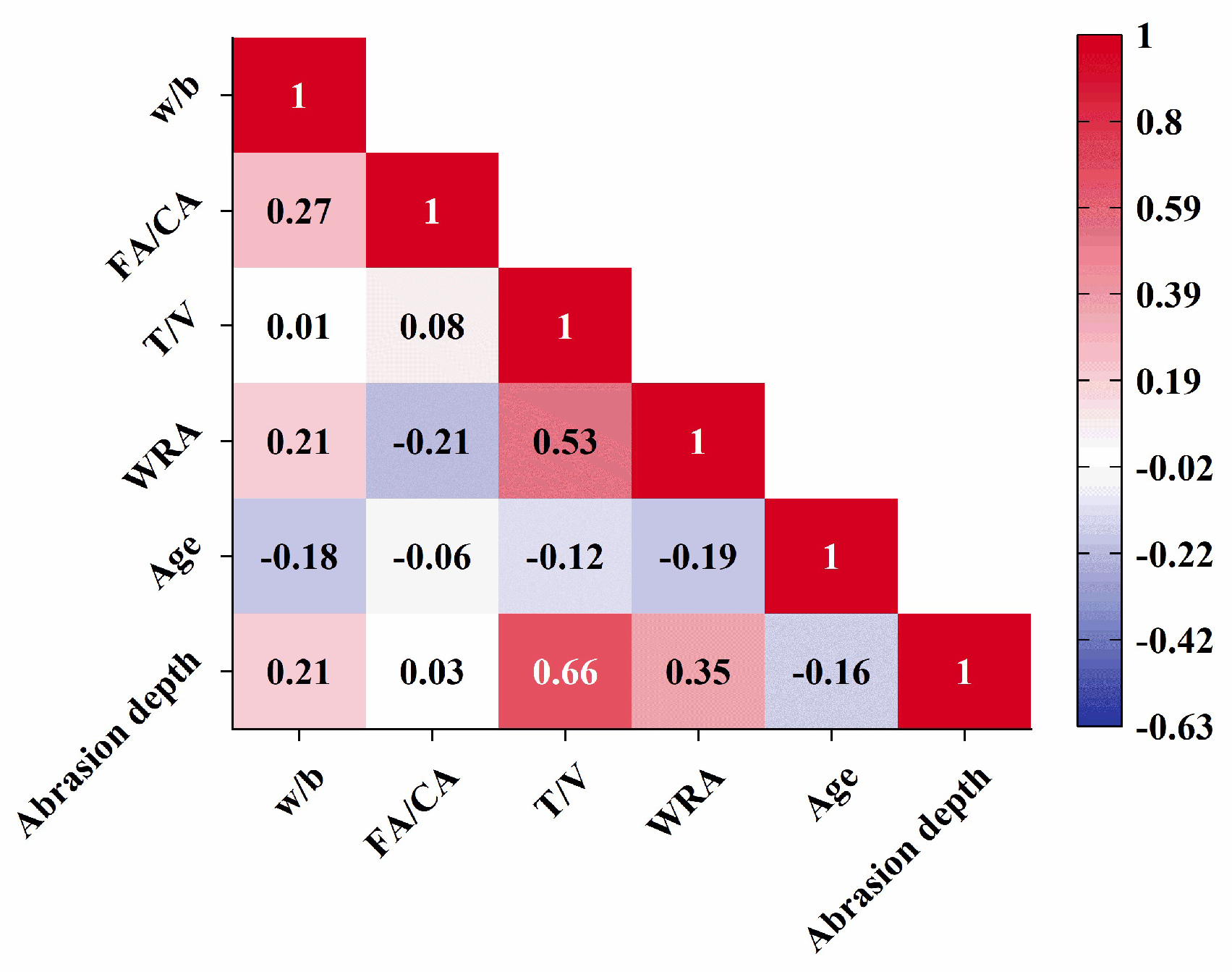
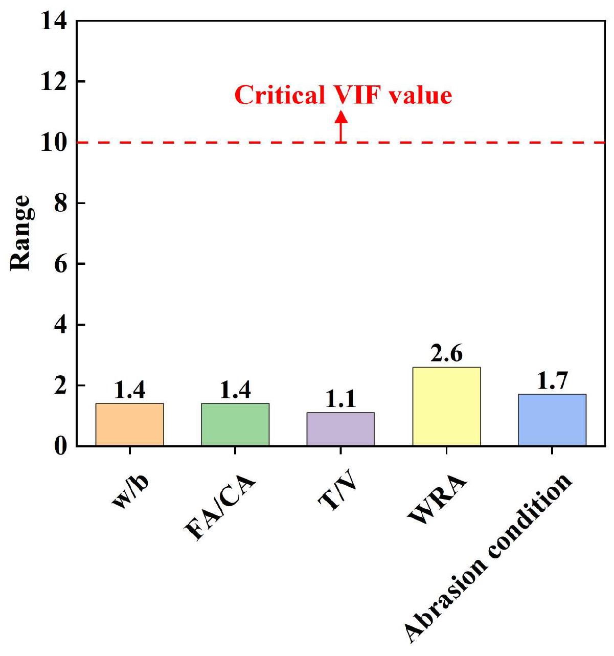
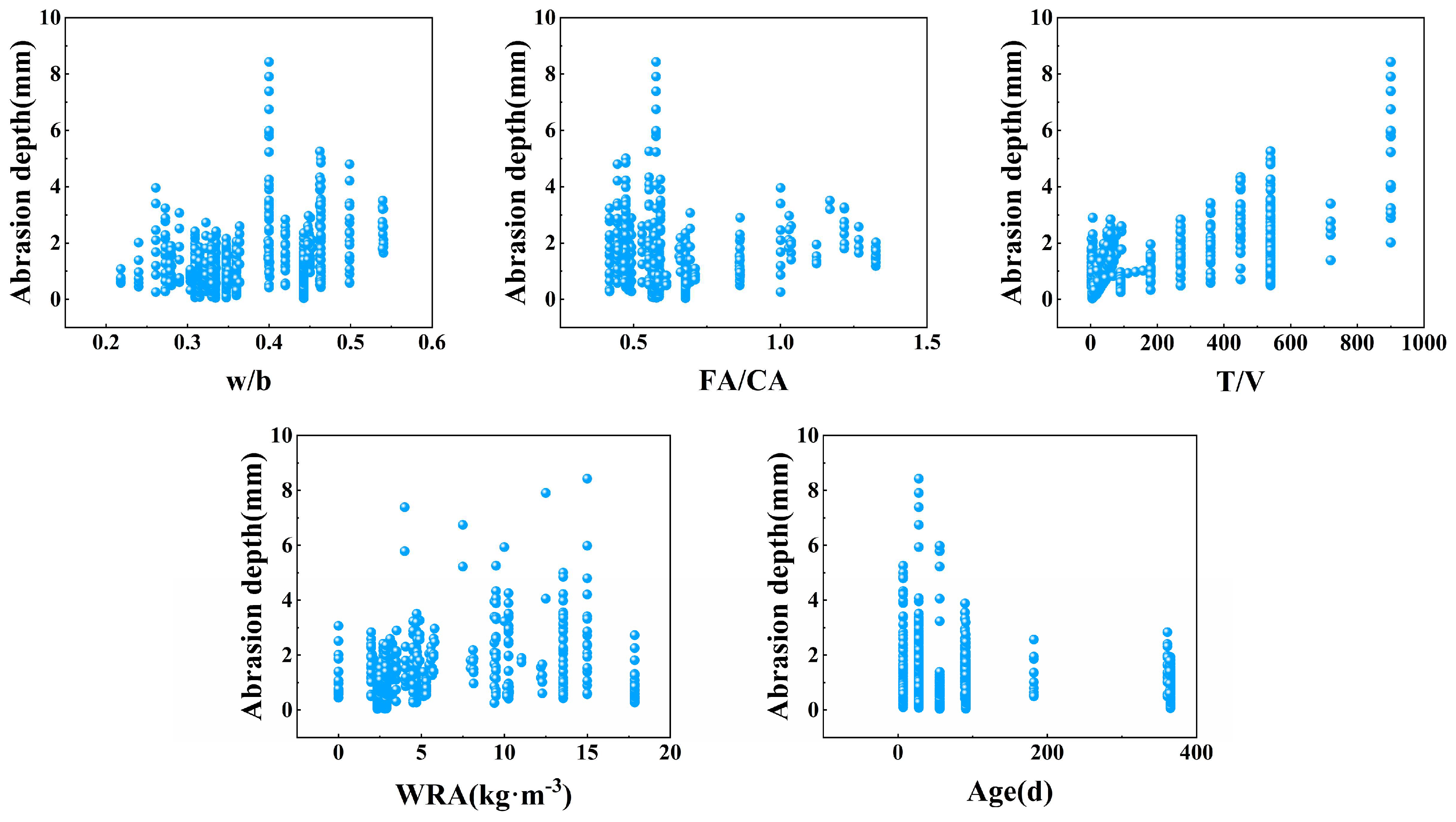
For combinations of features diagnosed with high collinearity, this study employs a feature reconstruction strategy. This involves constructing proportional relationships between features to replace the original independent features, thereby eliminating linear associations between variables. The specific processing methods included the following: for the collinear feature pair of fine aggregate content and coarse aggregate content, the two original independent content features were replaced with the ‘Ratio of Fine Aggregate to Coarse Aggregate Content (FA/CA)’; for the collinear feature pair of wear test duration and loading rate, the ‘Ratio of Wear Test Duration to Loading Rate (T/V)’ was constructed as a new feature. Following feature reconstruction, R and VIF were recalculated, yielding the results presented in Figure 5 and Figure 6. It can be observed that all correlations between features are below 0.7, and all VIF values are less than 10. Finally, the statistically analyzed dataset after feature reconstruction is shown in

Table 3. Distribution statistics of database after feature reconstruction.

	MEAN	STD	MIN	MID	MAX
w/b	0.38	0.07	0.22	0.36	0.54
FA/CA	0.63	0.17	0.42	0.58	1.33
T/V (s2/m)	9651.46	13,214.64	191	3000	54,000
WRA (kg/m3)	5.01	4.21	0	2.90	17.86
Age (d)	88.86	112.83	7	28	365
Ad (mm)	1.36	1.06	0.04	1.13	8.43

. Figure 7 displays a scatter plot of the data following feature reconstruction.

2.3. LightGBM

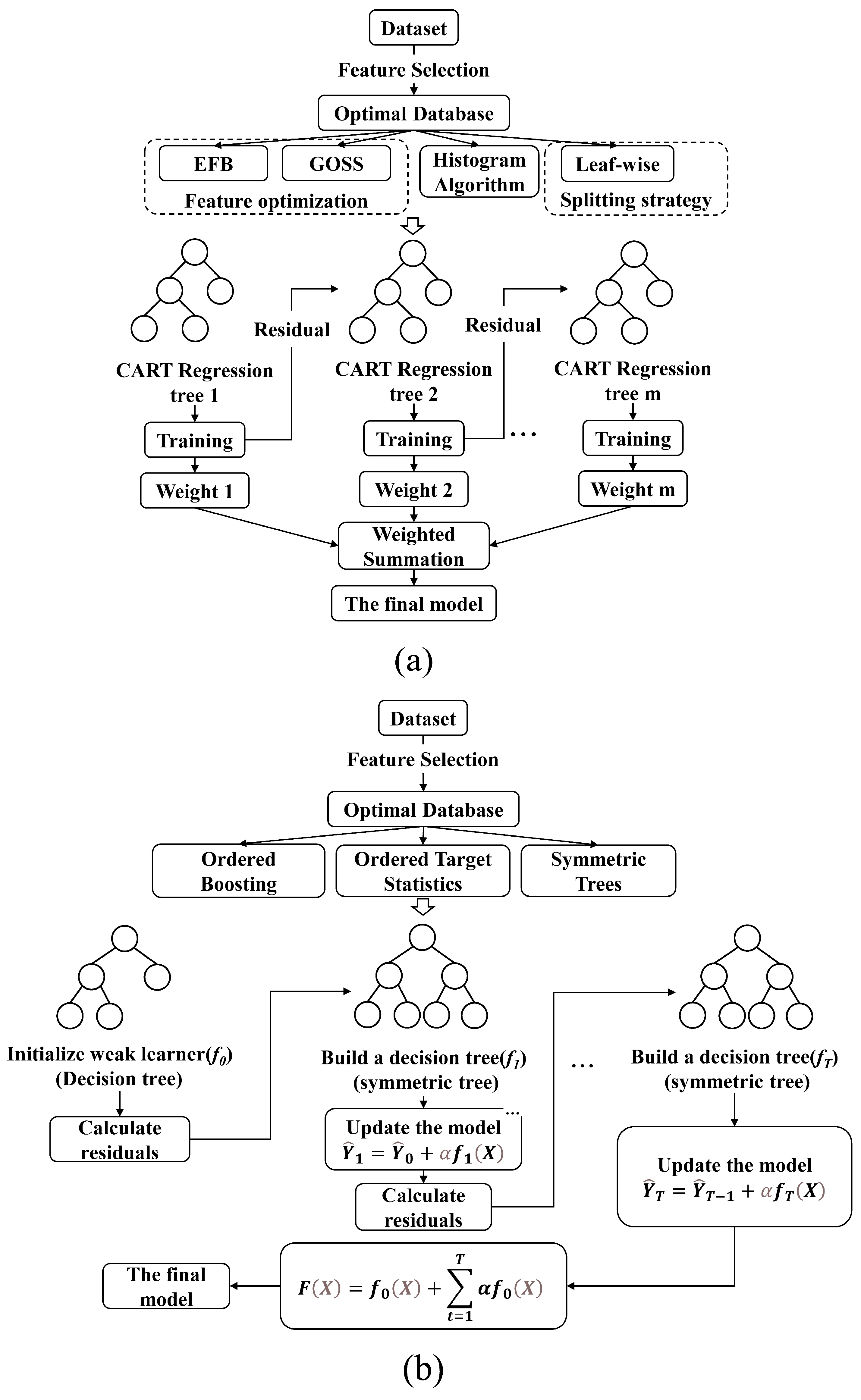
LightGBM (Light Gradient Boosting Machine) is an efficient gradient boosting framework based on decision tree ensembles, proposed by Microsoft in 2017 [40]. Its core design goal is to solve the problems of low training efficiency and high memory consumption of traditional gradient boosting decision trees (GBDTs) on large-scale datasets. When splitting, the LightGBM algorithm needs to pre-sort the original data of each feature, using a leaf-wise splitting method, i.e., each time splitting the leaf node with the maximum splitting gain among all leaves, while other leaf nodes are not split. The histogram algorithm “bins” the original feature data, dividing the data into different discrete intervals, and then traverses the discrete data to find the optimal split point. LightGBM retains samples with large absolute gradient values (high information gain) through Gradient-based One-Side Sampling (GOSS) and randomly discards some samples with small gradients, significantly reducing the data volume while maintaining model accuracy [40]. Assuming the sample gradient is $\nabla f$, the sampling strategy is to sort by absolute gradient values in descending order, retain the top a × 100% samples, randomly select b × 100% samples from the remaining, and multiply the sampled low-gradient samples by a weight (1 − a)/b when calculating information gain to compensate for distribution shifts. In addition, LightGBM uses Exclusive Feature Bundling (EFB) to merge mutually exclusive features (rarely taking non-zero values simultaneously) into a single feature, reducing the feature dimension [40]. Combining the above four technologies, the residual of one round of learner training is used as the input for the next round of learner training, i.e., the input data of each time depends on the output of the previous training, and the final model is obtained by weighted summation. As shown in Figure 8a, this algorithm is particularly suitable for regression and classification tasks with high-dimensional and large-scale datasets, and is widely used in big data modeling.

2.4. CatBoost

CatBoost (Categorical Boosting) is a gradient boosting framework proposed by the Russian Yandex team in 2017 [41]. It innovatively introduces Ordered Target Statistics and Symmetric Trees, significantly improving the efficiency of processing categorical data and the generalization ability of the model, becoming the preferred tool for handling heterogeneous data in industry [42]. CatBoost adopts a unique approach called “Ordered Target Statistics”, which calculates statistics of categorical features using data order information by sorting the data, thereby effectively integrating features into the model and avoiding the drawbacks of traditional encoding methods. It automatically generates interactive combinations of high-dimensional categorical features (such as $x_1\times x_2$) to enhance feature expression ability [43]. The algorithm uses a symmetric tree structure, which is a complete binary tree in form. When building a decision tree, for each node split, all possible feature and threshold combinations are considered, and all nodes at the same level of the tree have symmetric splitting methods. In the training process, first, a weak learner, usually a decision tree (whether symmetric or not), is initialized, and there is an error between the initial prediction value and the true value. In regression tasks, the residual of each sample is calculated, and the calculated residual is used as the new target value to build a new decision tree using the “symmetric tree structure”. The current model is updated based on the newly trained decision tree. This process is repeated, continuously training new decision trees and updating the model until the preset number of iterations is reached, the loss function converges to a certain extent, or other stopping conditions are met. Finally, the CatBoost model consists of multiple decision trees, and its prediction result is the sum of the prediction results of all decision trees, as shown in Figure 8b.

2.5. XGBoost

XGBoost (eXtreme Gradient Boosting) is a scalable tree boosting algorithm framework proposed by Chen and Guestrin in 2016 [44]. It significantly improves the efficiency and accuracy of gradient boosting algorithms in large-scale data scenarios through integrated decision tree models and parallel optimization technologies [44]. XGBoost (eXtreme Gradient Boosting) is a scalable tree boosting algorithm framework proposed by Chen and Guestrin in 2016. It significantly improves the efficiency and accuracy of gradient boosting algorithms in large-scale data scenarios through integrated decision tree models and parallel optimization technologies $\widehat{y_i}={\displaystyle {\sum }_{k=1}^K}{f}_k\left(x_i\right)$ (where K is the number of trees) through a weighted regularized objective function, and optimizes the following objectives through second-order Taylor expansion:

$$\mathcal{L}={\displaystyle {\sum }_{i=1}^n}l\left(y_i,\widehat{y_i}\right)+{\displaystyle {\sum }_{k=1}^K}\Omega \left(f_k\right)$$

(3)

where $\Omega \left(f_k\right)=\gamma T+{\displaystyle \frac{1}{z}}\lambda {‖\omega ‖}^2$ is the regularization term ($T$ is the number of leaf nodes, $\lambda$ is the leaf weight), and $\gamma$, $\lambda$ control the model complexity to suppress overfitting [44].

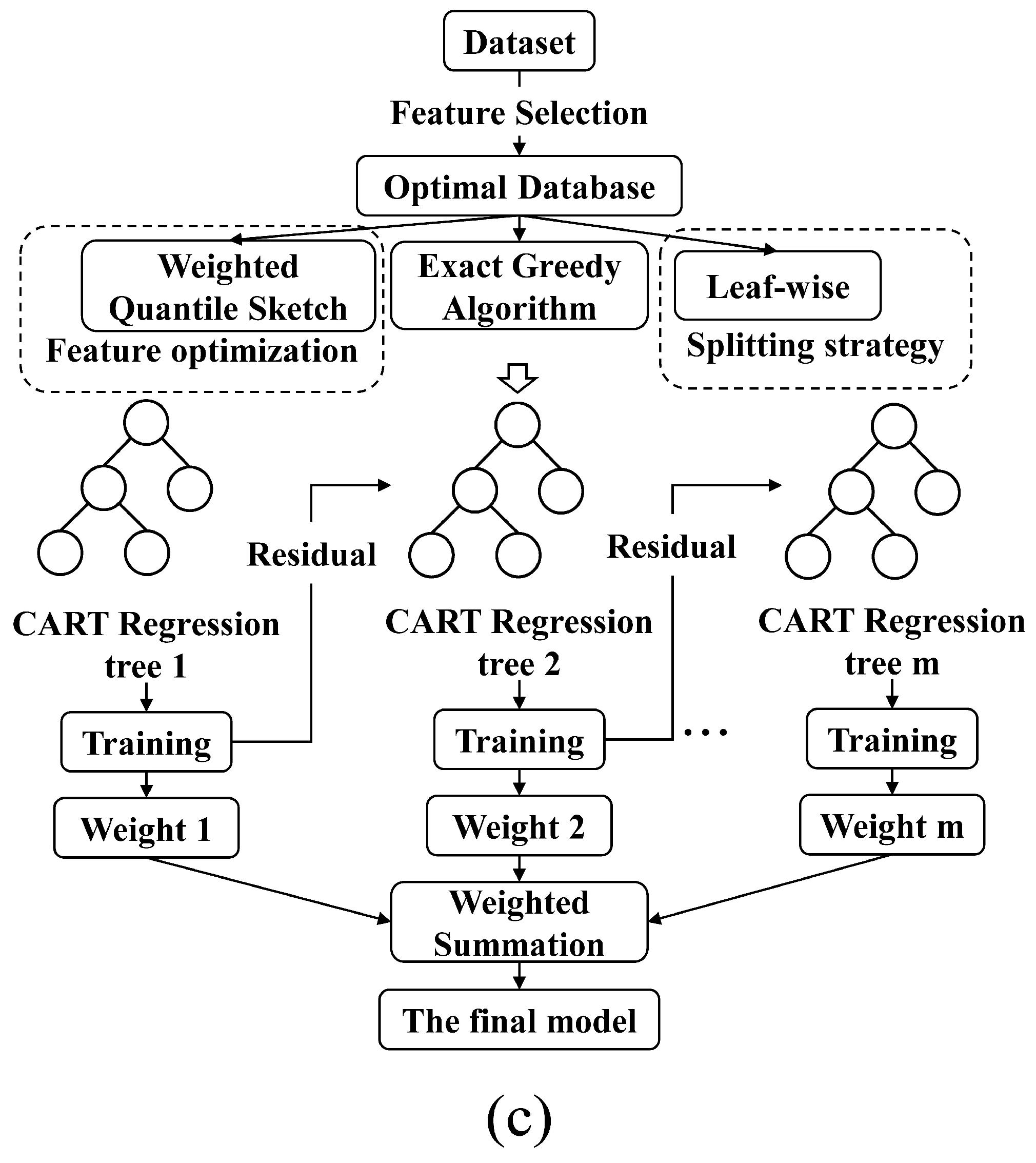
In split point optimization, the Exact Greedy Algorithm is used to traverse all feature split points; a Weighted Quantile Sketch approximation algorithm is introduced to sort feature values and bin them by gradient weight, reducing computational complexity. The node splitting gain formula is

$$G={\displaystyle \frac{1}{2}}\left[{\displaystyle \frac{{\left({\sum }_{i\in I_L}{g}_i\right)}^2}{{\sum }_{i\in I_L}{h}_i+\lambda }}+{\displaystyle \frac{{\left({\sum }_{i\in I_R}{g}_i\right)}^2}{{\sum }_{i\in I_R}{h}_i+\lambda }}-{\displaystyle \frac{{\left({\sum }_{i\in I}{g}_i\right)}^2}{{\sum }_{i\in I}{h}_i+\lambda }}\right]-\gamma$$

(4)

where $g_i={\partial }_{\widehat{y}}l\left(y_i,\widehat{y}\right){ \mathrm{and} h}_i={\partial }_y^{2}l\left(y_i,\widehat{y}\right)$ are the first and second derivatives of the loss function, and $I_L$ and $I_R$ are the left and right subsets after splitting. In the iteration stage, XGBoost is similar to LightGBM, with a flowchart shown in Figure 8c.

2.6. Genghis Khan Shark Optimizer

Genghis Khan Shark Optimizer, also called GKS Optimizer (GKSO), is a new nature-inspired MA (meta-heuristic algorithm) based on the behavior of Genghis Khan Sharks (GKS), used for numerical optimization and engineering design. It was proposed by Hu et al. [24] in 2023. GKSO is inspired by the predation and survival behaviors of GKS, and the entire optimization process is realized by simulating four different activities of GKS: hunting (exploration), moving (exploitation), foraging (switching from exploration to exploitation), and self-protection mechanisms [24].

(a) In the GKSO algorithm, to simulate the hunting stage of GKS, random positions are generated as “optimal hunting sites” constrained by the upper and lower bounds (ULB) of the search space. The individual position is updated according to Equation (5) [24]:

$$\begin{array}{cc}\hfill X_i^j(t+1)& =X_i^j(t)+{\displaystyle \frac{l{b}_j+r_1(u{b}_j-l{b}_j)}{it}}, i=\mathrm{1,2},\dots ,N, j=\mathrm{1,2},\dots ,D,it\hfill \\ & =\mathrm{1,2},\dots ,T.\hfill \end{array}$$

(5)

where $X_i^j(t+1)$ represents the position of the i-th member in the j-th dimension at time t + 1, ub_j and lb_j are the ULB in the j-th dimension, respectively. $r_1$ is a random number in the interval [0, 1], N is the population size, D is the problem dimension, it is the current iteration count, and T is the total number of iterations [24].

(b) GKS usually relies on its keen sense of smell to continuously approach high-quality prey, which is simulated by Equation (6) [24]:

$${\widehat{X}}_i^j\left(t+1\right)=s^{*}\left(X_{best}^j\left(t\right){-X}_i^j\left(t\right)\right)$$

(6)

where $X_{best}^j\left(t\right)$ is the known optimal hunting position in the j-th dimension at time t, and s is the olfactory intensity of GKS when moving towards the optimal prey, which depends on the concentration of odor emitted by the prey [24]. This model is established as follows:

$$s=m{I}^r$$

(7)

where r is a random number in the interval [0, 1], reflecting the absorption of prey odor by the search agent. For two extreme cases, when r = 0, it means that the odor emitted by the prey is completely undetectable to GKS, and the search agent will re-enter the exploration stage; when r = 1, this odor is completely absorbed by GKS, so the algorithm may easily reach the optimal value (possibly local) [24]. Therefore, parameter r controls the behavior of GKS; I is an attribute intensity, which depends on the ability of individual populations, i.e., the current fitness value of each agent; m is a non-negative constant and a key parameter affecting the convergence rate of GKSO, and also the only control parameter in GKSO [24].

(c) Fish use various strategies for foraging. Tuna in TSO arrange themselves in a parabolic shape for cooperative feeding [45]. GKS has the same habit and will launch a fatal attack on high-quality prey through an overall parabolic process. The mathematical model established accordingly is shown in Equation (7):

$$X_i^j\left(t+1\right)=X_{best}^j\left(t\right)+r_2\left(X_{best}^j\left(t\right){-X}_i^j\left(t\right)\right)+\lambda p^2\left(X_{best}^j\left(t\right){-X}_i^j\left(t\right)\right)$$

(8)

where $r_2$ is a random number in [0, 1], $\lambda$ is a random number of 1 or −1, and p is a parameter controlling the movement step size of GKS during its activities.

(d) During foraging, GKS may be attacked by natural enemies. To cope with this, GKS has a color-changing mechanism: when frightened, the color of its tail and body becomes brighter, thereby deterring predators and escaping quickly. The model simulating this behavior is Equation (10):

$$\left\{\begin{array}{cc}\hfill X_i^j\left(t+1\right)=X_i^j\left(t\right)& + k_1\left({a_{1}X}_{best}^j\left(t\right){-a_{2}X}_k^j\left(t\right)\right)+k_2\rho \left(a_3\left({X2}_i^j\left(t\right){-X1}_i^j\left(t\right)\right)\right)\hfill \\ & +{\displaystyle \raisebox{1ex}{$ a_2\left(X_{u1}\left(t\right)-X_{u2}\left(t\right)\right)$}\!\left/ \!\raisebox{-1ex}{$2$}\right.}, if a_1<0.5\hfill \\ \hfill X_i^j\left(t+1\right)=X_{best}^j\left(t\right)& + k_1\left({a_{1}X}_{best}^j\left(t\right){-a_{2}X}_k^j\left(t\right)\right)-k_2\rho \left(a_3\left({X2}_i^j\left(t\right){-X1}_i^j\left(t\right)\right)\right)\hfill \\ & + {\displaystyle \raisebox{1ex}{$a_2\left(X_{u1}\left(t\right)-X_{u2}\left(t\right)\right)$}\!\left/ \!\raisebox{-1ex}{$2$}\right.}, otherwise\hfill \end{array}\right.$$

(9)

2.7. Hyperparameter Optimization

This study used GKSO to optimize the hyperparameters of LightGBM, CatBoost, and XGBoost. Prior to model training, the multi-source database comprising 690 case groups underwent data partitioning: it was randomly split in an 8:2 ratio into a training set (552 groups, accounting for 80%) and a test set (138 groups, accounting for 20%). The training set facilitated model parameter learning and hyperparameter optimization, whilst the test set served as an independent validation of the model’s generalization capability, thereby preventing data leakage from interfering with prediction outcomes.

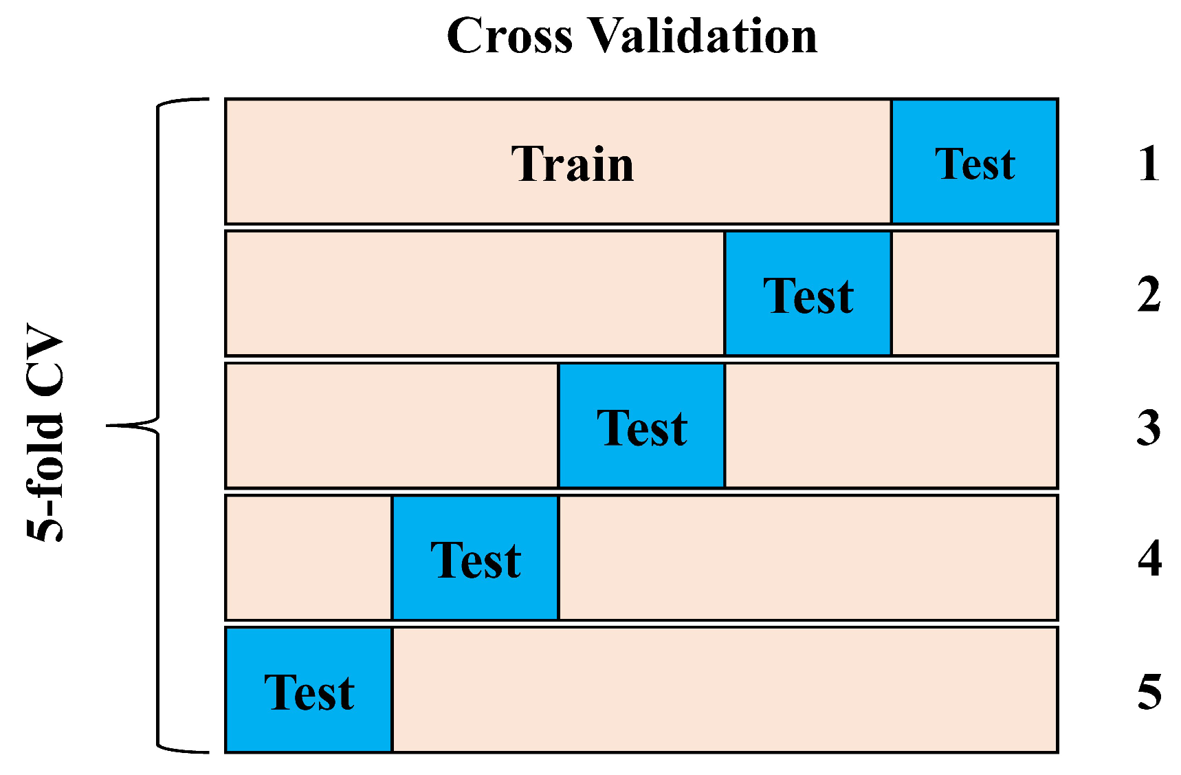
In stage (b) of GKSO in Section 2.6, m affects the optimal search ability of the algorithm, so it is necessary to select the most appropriate m value for hyperparameter optimization. Therefore, referring to the relevant optimization results in Reference [24], six groups of m = 0.5, m = 1, m = 1.5, m = 2, m = 2.5, and m = 3 were selected to test the optimal m. Thus, three groups of hybrid ensemble models were formed: GKSO-LightGBM, GKSO-CatBoost, and GKSO-XGBoost. Each group of models performed hyperparameter optimization under different m values, using 5-fold cross-validation, with the average MSE as the fitness function, after 500 iterations. The principle of five-fold cross-validation involves randomly partitioning the training dataset into five subsets of similar size. Four subsets are cyclically employed as training data, while one serves as the validation subset. The average performance across five validation rounds constitutes the model’s evaluation metric for that parameter configuration. This approach effectively mitigates random errors inherent in single training–validation splits and prevents overfitting. The specific steps are as follows: First, the 552 training sets are randomly and evenly distributed across 5 folds (with each fold containing 110–111 datasets). Then, folds 1–4 are used as the training data and fold 5 as the validation data to train the model and calculate the MSE. Subsequently, the validation fold is cyclically swapped (sequentially using folds 5-4, 5-3, 5-2, and 5-1 as validation data), repeating the training and MSE calculation process. Finally, the average of the five MSE values is taken as the fitness function value for the model under the current m value. After 500 iterations, the hyperparameter combination yielding the smallest fitness function value is selected as the optimal parameters for the corresponding model. The process is shown in Figure 9.

2.8. Performance Evaluation

This study used four performance metrics to evaluate the three established hybrid ensemble models: R², MSE, RMSE, and VAF.

The coefficient of determination (R²—R-squared) measures the model’s ability to explain the variability of data, representing the proportion of the variance of the target variable that can be explained by the independent variables. Its value range is [0, 1], and a value closer to 1 indicates a better model fit. The calculation formula is shown in Equation (10):

$$R^2=1-{\displaystyle \frac{{\sum }_{i=1}^n{\left(y_i-\widehat{y_i}\right)}^2}{{\sum }_{i=1}^n{\left(y_i-\overline{y}\right)}^2}}$$

(10)

The mean absolute error (MAE) directly represents the average absolute deviation between the predicted and true values, with the same unit as the target variable. Compared with the RMSE, it does not have a squared amplification effect on outliers. The calculation formula is shown in Equation (11):

$$MAE={\displaystyle \frac{1}{n}}{\sum }_{i=1}^n\left|y_i-\widehat{y_i}\right|$$

(11)

The root mean square error (RMSE) measures the deviation between predicted and true values, is sensitive to outliers, and a smaller value indicates a better model.

$$RMSE=\sqrt{{\displaystyle \frac{1}{n}}{\sum }_{i=1}^n{\left(y_i-\widehat{y_i}\right)}^2}$$

(12)

The variance accounted for (VAF) measures the proportion of variance explained between the model’s predicted values and true values, independent of data scale.

$$VAF=\left(1-{\displaystyle \frac{\mathit{var}\left(y-\widehat{y}\right)}{var\left(y\right)}}\right)\times 100$$

(13)

In the above formulas, n is the total number of samples, $y_i$ is the model-predicted abrasion depth, $\widehat{y_i}$ is the measured abrasion depth, and $\overline{y}$ is the average of the experimental data.

3. Results and Discussion

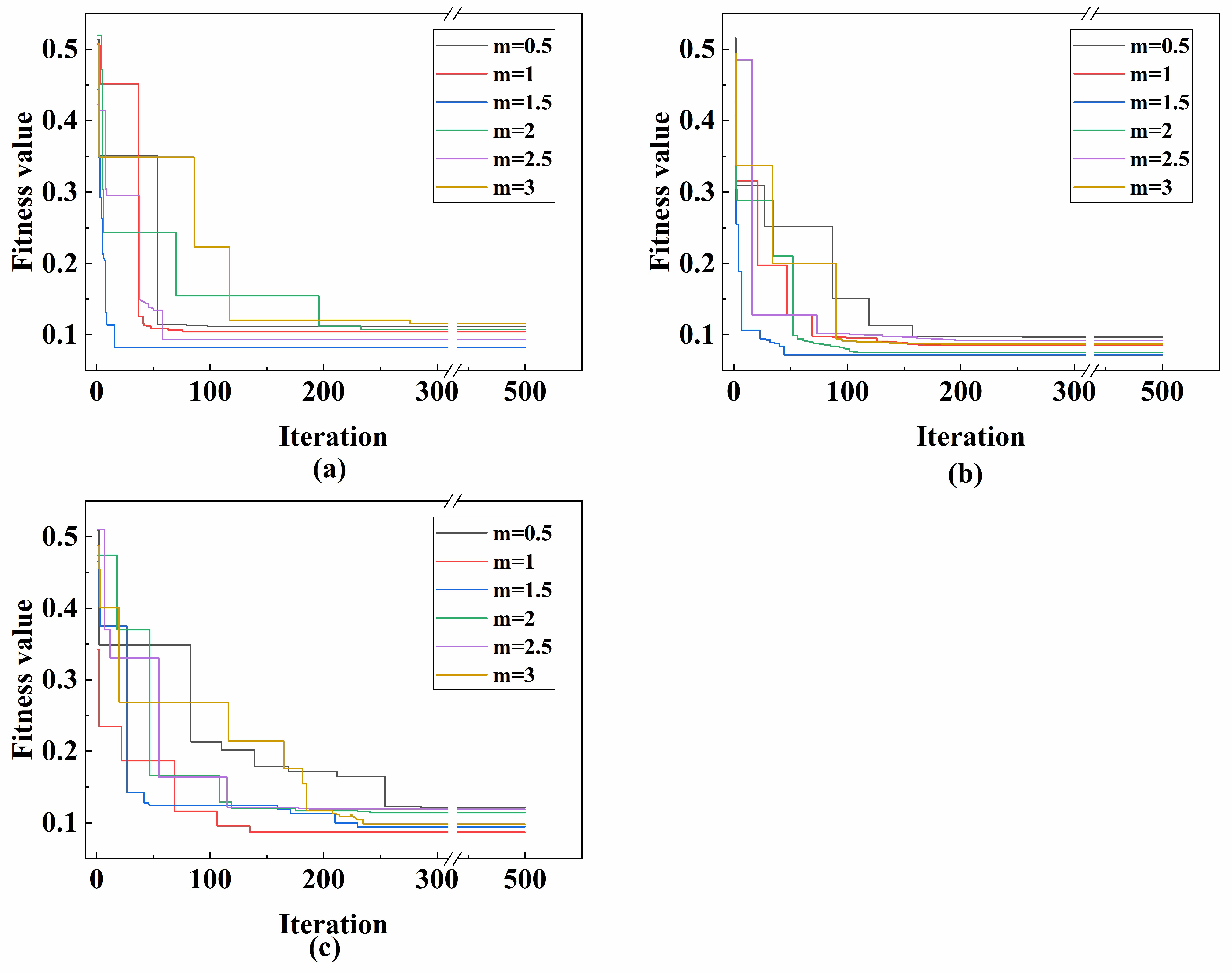
Figure 8 shows the iteration curves of the three groups of models after hyperparameter optimization. Figure 10a is the iteration curve of six GKSO-LightGBM models; Figure 10b is that of six GKSO-CatBoost models; Figure 10c is that of six GKSO-XGBoost models. It can be seen from the figures that all models reached the minimum fitness value before 300 iterations. GKSO-CatBoost had the best optimization effect overall, and GKSO-LightGBM and GKSO-CatBoost had faster convergence rates than GKSO-XGBoost. Among the six GKSO-LightGBM models, the m = 1.5 group performed best; among the six GKSO-CatBoost models, the m = 1.5 group performed best; among the six GKSO-XGBoost models, the m = 1 group performed best. In actual prediction applications, the corresponding m values can be prioritized.

Table 4. Final fitness values of models after hyperparameter optimization under different m values.

	Fitness Value
m	GKSO-LightGBM	GKSO-CatBoost	GKSO-XGBoost
0.5	0.1121	0.0972	0.1216
1	0.1044	0.0858	0.0871
1.5	0.0818	0.0718	0.0944
2	0.1073	0.0758	0.1143
2.5	0.0934	0.0922	0.1193
3	0.1163	0.0873	0.0984

shows the final fitness values of GKSO-LightGBM, GKSO-CatBoost, and GKSO-XGBoost after hyperparameter optimization under different m values.

Table 5. GKSO-LightGBM prediction results.

Train Set
m	R2	MAE	RMSE	VAF
0.5	0.9923	0.0891	0.0942	99.23
1	0.994	0.0769	0.0831	99.4
1.5	0.9989	0.0193	0.0356	99.89
2	0.9958	0.0447	0.0689	99.58
2.5	0.9988	0.0203	0.0359	99.88
3	0.9893	0.1023	0.1108	98.93
Test set
m	R2	MAE	RMSE	VAF
0.5	0.953	0.1472	0.2172	95.30
1	0.9582	0.1426	0.2063	95.82
1.5	0.9794	0.1249	0.1579	97.95
2	0.9638	0.1363	0.1904	96.39
2.5	0.9737	0.1301	0.1735	97.38
3	0.9491	0.1516	0.2272	94.93

,

Table 6. GKSO-CatBoost prediction results.

Train Set
m	R2	MAE	RMSE	VAF
0.5	0.995	0.0556	0.0745	99.50
1	0.9981	0.0324	0.0490	99.81
1.5	0.9990	0.0182	0.0350	99.90
2	0.9956	0.0551	0.0713	99.56
2.5	0.9981	0.0294	0.0490	99.81
3	0.9979	0.0385	0.0505	99.79
Test set
m	R2	MAE	RMSE	VAF
0.5	0.9502	0.1499	0.2234	95.02
1	0.9724	0.1276	0.1661	97.24
1.5	0.9824	0.1151	0.1231	97.91
2	0.9631	0.1260	0.1611	96.31
2.5	0.9798	0.1244	0.1562	97.99
3	0.9691	0.1209	0.1446	96.91

and

Table 7. GKSO-XGBoost prediction results.

Train Set
m	R2	MAE	RMSE	VAF
0.5	0.9907	0.0804	0.102	99.07
1	0.9975	0.0301	0.0552	99.75
1.5	0.9973	0.0311	0.056	99.73
2	0.9955	0.656	0.0745	99.55
2.5	0.9942	0.0768	0.0823	99.42
3	0.9958	0.0546	0.0681	99.58
Test set
m	R2	MAE	RMSE	VAF
0.5	0.9504	0.1496	0.2227	95.05
1	0.9772	0.1276	0.166	97.72
1.5	0.9734	0.1192	0.1386	97.34
2	0.9587	0.1473	0.2175	95.89
2.5	0.9558	0.1443	0.2104	95.63
3	0.9673	0.1230	0.1517	96.74

show the model prediction results of the three groups under different m values. Table 5 shows the prediction results of GKSO-LightGBM under different m values, Table 6 shows those of GKSO-CatBoost, and Table 7 shows those of GKSO-XGBoost. The data in the tables indicate that consistent with the convergence results of the average MSE during iteration, among the six GKSO-LightGBM models, the m = 1.5 group had the best prediction results; among the six GKSO-CatBoost models, the m = 1.5 group performed best; among the six GKSO-XGBoost models, the m = 1 group performed best. After obtaining the above results, the corresponding hyperparameter combinations were extracted, as shown in

Table 8. Hyperparameter combinations.

Models	Hyperparameters	Values
GKSO-LightGBM	n_estimators	666
	learning_rate	0.2039
	min_child_samples	5
	num_leaves	20
	m	1.5
	Iterations (CV)	500
GKSO-CatBoost	Iterations	796
	learning_rate	0.4060
	depth	3
	l2_leaf_reg	10
	m	1.5
	Iterations (CV)	500
GKSO-XGBoost	n_estimators	981
	learning_rate	0.2985
	max_depth	4
	colsample_bytree	0.1791
	m	1
	Iterations (CV)	500

. Comparing the optimized prediction results of the same model under different m values, it is not difficult to find that the m = 1.5 group performed excellently. Although for the XGBoost group, the optimization result of the m = 1 group was better than that of m = 1.5, the difference in R² between the training set and test set was less than 0.01. Therefore, m = 1.5 can be set as the optimal value, which is consistent with the relevant results in Reference [46], proving the feasibility of GKSO algorithm optimization.

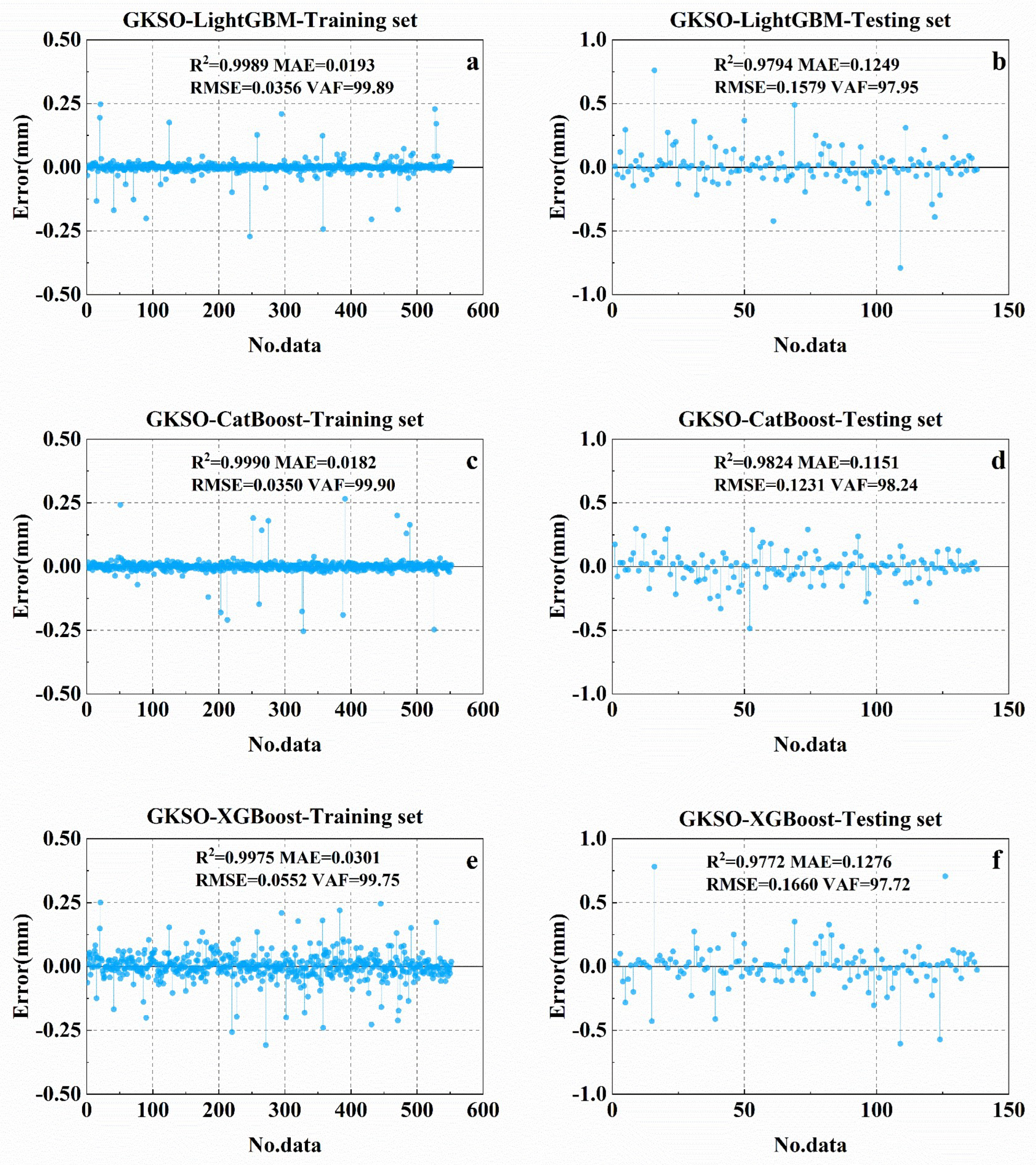
Figure 11 is the error plot of the three hybrid models, where the error is the difference between the true value and the predicted value. For the error performance of the three hybrid models on the training set, the errors are all less than 0.4 mm, indicating that each hybrid model has excellent performance in predicting abrasion depth on the training set. On the training set, the error points of the XGBoost group are significantly less concentrated near the x-axis than those of the LightGBM and CatBoost groups, but overall, they still show low errors. For the LightGBM and CatBoost groups on the training set, the error points are concentrated near the x-axis, with only a few points having errors exceeding 0.25. This indicates the high accuracy of these two hybrid models. On the test set, all errors of the three hybrid models are less than 1 mm. For the LightGBM group, less than 2% of the prediction results have errors higher than 0.5 mm, 8.7% have errors higher than 0.25 mm, and approximately 71% have errors lower than or equal to 0.1 mm. For the XGBoost group, approximately 3% of the prediction results have errors higher than 0.5 mm, 8% have errors higher than 0.25 mm, and 65% have errors lower than or equal to 0.1 mm. For the CatBoost group, 0.72% of the prediction results have errors higher than 0.5 mm, 6.5% have errors higher than 0.5 mm, and 74% have errors lower than or equal to 0.1 mm. Therefore, by comparison, the GKSO-CatBoost model is significantly superior to other models in correcting high-error predictions and has the best error performance; in terms of prediction errors between 0.25 and 0.5, GKSO-LightGBM has 1.7% more than GKSO-XGBoost, but in other ranges, GKSO-LightGBM has better performance.

3.1. Model Comparison and Selection

Table 9. Score performance of different models.

Model	R2	Score	MAE	Score	RMSE	Score	VAF (%)	Score	Total
Train Set
GKSO-LightGBM	0.9989	8	0.0193	8	0.0356	8	99.89	8	32
GKSO-CatBoost	0.9990	9	0.0182	9	0.0350	9	99.90	9	36
GKSO-XGBoost	0.9975	6	0.0301	6	0.0552	6	99.75	6	24
Bayes-LightGBM	0.9821	4	0.1211	4	0.2031	4	98.21	4	12
Bayes-CatBoost	0.9816	3	0.1306	2	0.2317	2	98.16	3	13
Bayes-XGBoost	0.9794	2	0.1451	1	0.2298	3	97.94	2	8
LightGBM	0.9437	1	0.1216	3	0.2561	1	94.36	1	6
CatBoost	0.9943	5	0.0424	5	0.0609	5	99.43	5	20
XGBoost	0.9980	7	0.0201	7	0.0406	7	99.80	7	28
Test set
GKSO-LightGBM	0.9794	8	0.1249	8	0.1579	8	97.95	8	32
GKSO-CatBoost	0.9824	9	0.1151	9	0.1231	3	98.24	9	36
GKSO-XGBoost	0.9772	7	0.1276	7	0.1660	7	97.72	7	28
Bayes-LightGBM	0.9687	5	0.1349	4	0.1781	4	96.87	5	18
Bayes-CatBoost	0.9702	6	0.1303	5	0.1692	6	97.02	6	23
Bayes- XGBoost	0.9646	4	0.1421	3	0.1769	5	96.46	4	16
LightGBM	0.9246	2	0.1739	1	0.2561	1	92.46	2	4
CatBoost	0.9485	3	0.1292	6	0.2338	3	94.85	3	15
XGBoost	0.9215	1	0.1555	2	0.2541	2	92.16	1	6

shows the prediction results and comprehensive scores of nine models, including models optimized by GKSO, models optimized by Bayes, and models with default parameters. The results indicate that on both the training and test sets, GKSO-CatBoost obtained the highest score of 36; GKSO-LightGBM was slightly inferior to GKSO-CatBoost, ranking second, with 32 points on both sets; LightGBM with default parameters obtained the lowest score, with 6 points on the training set and 4 points on the test set. Observing the same model under different hyperparameter optimization schemes, for each model, the prediction results under default parameters are poor; after hyperparameter optimization by the Bayes algorithm, the R² and VAF of the LightGBM model on the training and test sets increased, and MAE and RMSE decreased, with the most significant optimization range of RMSE on the test set, approximately 43.8%; however, the R² and VAF of CatBoost and XGBoost on the training set did not increase but decreased, and MAE and RMSE on the training set increased, with no abnormal performance on the test set, reflecting that the model under default parameters has overfitting, and excessive learning leads to poor performance on the test set. After hyperparameter optimization by the GKSO algorithm, all performance indicators of each model improved positively, with better performance improvement on both the training and test sets than the Bayes algorithm, narrowing the gap in performance indicators between the training and test sets and effectively preventing the model from overfitting, thus avoiding insufficient prediction accuracy.

3.2. Model Feasibility Verification

To validate the feasibility of the abrasion depth prediction model, experimental data from additional literature sources were screened [46]. Data from experimental groups matching the model’s input characteristics FA/CA, T/V, w/b, WRA, and age) to ensure complete alignment between input variables and model design, thereby establishing a robust data foundation for subsequent prediction validation.

In all experimental groups, aggregate quantities were fixed (coarse aggregate ‘stone’ at 1263 kg/m³, fine aggregate ‘sand’ at 569 kg/m³). Water-reducing agent (WRA) was not added separately (considered 0%). The curing period was uniformly set at 28 days (standard curing age). Abrasion testing was conducted according to ASTM C1138M-19 [47] (underwater steel ball method), with loading rates converted via the device’s rotational parameters. Specific input characteristic data is as follows:

(1)

FA/CA: The aggregate (fine aggregate) consumption for all mix designs is 569 kg/m³, and the stone (coarse aggregate) consumption is 1263 kg/m³. Calculated by mass ratio, FA/CA = 569/1263 ≈ 0.45 (fixed value, no variation between mix designs).

(2)

T/V: Based on the ASTM C1138M-19 apparatus parameters, the rotational angular velocity $W_r$ = 0.36 rad/s, and the steel ball’s radius of motion $R_a=5.4~15.5 \mathrm{c}\mathrm{m}$, calculated using Formula (4) and taking the average radius of 10 cm, the velocity is converted to V = 0.036 m/s.

Ultimately, T/V = 120,000 s²/m.

(3)

w/b: Experimental settings: Three gradients of 0.35, 0.40, and 0.45 were employed as core variables for model input. The specific values for each group are detailed in Table 10.

(4)

WRA: No additional water-reducing agent was added to the experiment; all groups had WRA = 0%.

(5)

Age: All specimens were standard-cured for 28 days; age = 28 days.

The wear depth was measured using a three-dimensional topography scanning system (5 mm point spacing, 400 points per specimen). The final selection yielded data corresponding to the input characteristics and abrasion depth for three core experimental groups, as shown in Table 10. All data points exhibiting parallel specimen deviations exceeding 10% were excluded to ensure reliability. Using GKSO-Catboost to input and predict the aforementioned three datasets yielded the results shown in Table 11. The table also calculates the RE (relative error) between the predicted and actual values. The results indicate that the error in all predictions is less than or equal to 13.6%, falling within the acceptable range for engineering purposes and confirming the practicality of the GKSO-CatBoost approach.

Table 10. Model input features and documented abrasion depth measurement data.

Group	w/b	FA/CA	T/V	WRA	Age	Ad
1	0.35	0.45	120,000	0	28	6.71
2	0.40	0.45	120,000	0	28	6.65
3	0.45	0.45	120,000	0	28	8.46

Table 10. Model input features and documented abrasion depth measurement data.

Group	w/b	FA/CA	T/V	WRA	Age	Ad
1	0.35	0.45	120,000	0	28	6.71
2	0.40	0.45	120,000	0	28	6.65
3	0.45	0.45	120,000	0	28	8.46

Table 11. GKSO-Catboost Prediction Results.

Group	w/b	FA/CA	T/V	WRA	Age	Ad (Pre)	RE
1	0.35	0.45	120,000	0	28	7.62	13.6%
2	0.40	0.45	120,000	0	28	5.85	12.0%
3	0.45	0.45	120,000	0	28	7.66	9.5%

Table 11. GKSO-Catboost Prediction Results.

Group	w/b	FA/CA	T/V	WRA	Age	Ad (Pre)	RE
1	0.35	0.45	120,000	0	28	7.62	13.6%
2	0.40	0.45	120,000	0	28	5.85	12.0%
3	0.45	0.45	120,000	0	28	7.66	9.5%

3.3. SHAP Result Analysis

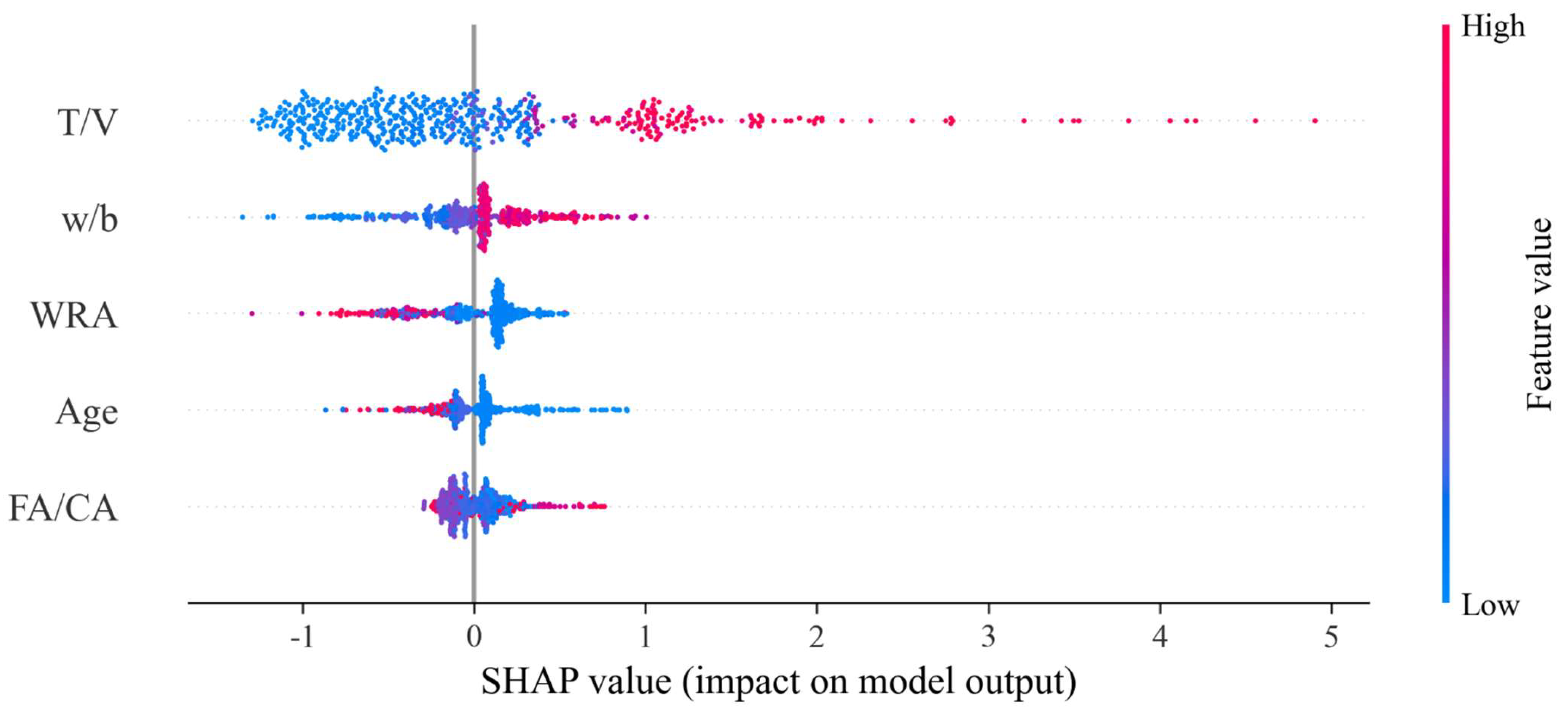
SHAP is crucial for understanding the contribution and interaction of each feature in the model, providing insights to enhance interpretability and improve feature selection [48]. This study extracted the SHAP global importance plot of the optimal model GKSO-CatBoost, as shown in Figure 12. In the figure, blue points represent low feature values, red points represent high feature values, and purple points represent feature values between the two, with color depth corresponding to the value within the interval. The figure indicates that T/V has the greatest impact on the model output, followed by w/b, WRA, age, and FA/CA. T/V is positively correlated with abrasion depth overall, with the largest SHAP value range, and high T/V values often have a positive impact on the model’s predicted abrasion depth. An increase in the T/V ratio means that the material withstands higher abrasion energy per unit time. Longer test time or higher loading speed will lead to an increase in cumulative abrasion. This is consistent with physical laws, as abrasion depth is positively correlated with load action time and kinetic energy input. w/b shows a more obvious positive correlation with model prediction, with high w/b values distributed in the positive SHAP value region and low w/b values in the negative region, and the distribution range of points is significantly smaller than that of T/V. An increase in w/b reduces concrete compactness and increases capillary porosity, which will lead to a more fragile ITZ (interface transition zone), reduced bond strength between aggregate and paste, and easier paste spalling and aggregate pull-out during abrasion. Therefore, the abrasion resistance of high w/b concrete decreases significantly. For WRA, high WRA values are concentrated in the negative SHAP value region, and low WRA values are distributed in both positive and negative SHAP value regions, with a complex relationship with SHAP values. Similarly, the distribution characteristics of age have a complex relationship with SHAP values, but it is worth noting that high ages are concentrated in the negative SHAP value region, corresponding to a reduction in predicted abrasion depth in the model. Under normal curing, a longer age will lead to higher compressive strength in concrete. According to the empirical formula: abrasion depth $\propto 1/\sqrt{f_c}$, it can be inferred that the model correctly identifies the relationship between features and true output. For FA/CA, there is no obvious monotonic relationship between high/low feature values and SHAP values, but high and low value points are scattered in positive and negative regions. It can be seen that an appropriate FA/CA can optimize the gradation, enhance skeleton compactness, and improve abrasion resistance.

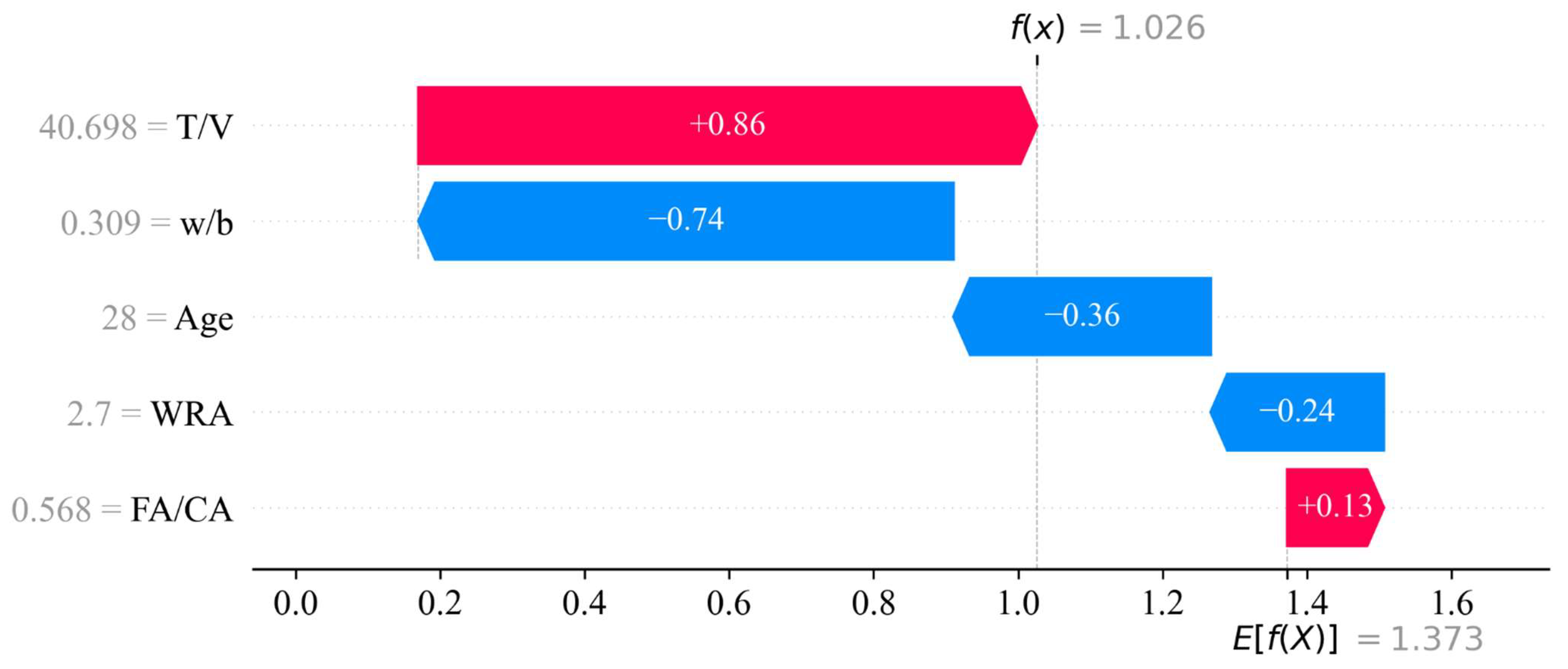
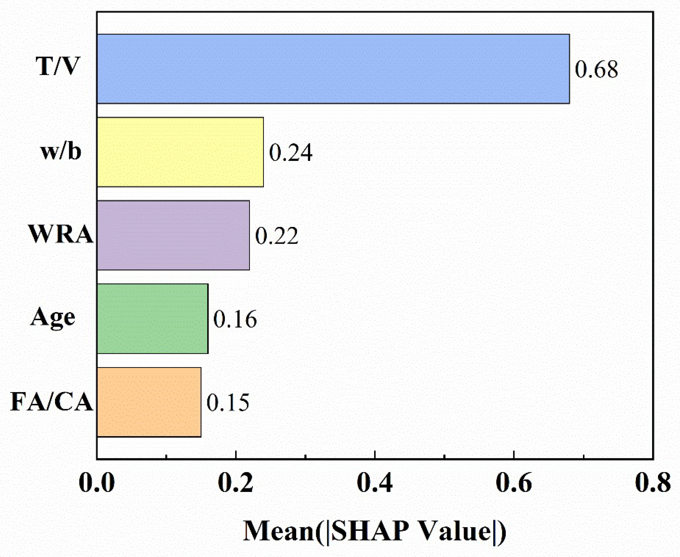
Figure 13 shows the feature contribution decomposition for the model’s prediction of concrete abrasion depth. In the figure, the predicted value (f(x)) is 1.026 mm, and the baseline value (E[f(X)]) is 1.373 mm. The measured abrasion depth of this case is 1.650 mm. The contribution of each feature to this case is ranked as T/V, w/b, age, WRA, and FA/CA, with SHAP values of 0.86, −0.74, −0.36, −0.24, and 0.13, respectively. Figure 14 shows the feature importance ranking explained by SHAP, where T/V has the highest importance of 0.68, followed by w/b, age, WRA, and FA/CA. T/V is significantly higher than the other four features, dominating the model’s prediction output.

4. Research Significance and Limitations

This study constructed a high-precision prediction model for concrete abrasion depth in hydraulic tunnels based on the combination of meta-heuristic algorithms and ensemble learning. By introducing GKSO to optimize the hyperparameters of three mainstream gradient boosting frameworks (LightGBM, XGBoost, and CatBoost) and adopting K-fold cross-validation, the risk of overfitting was effectively reduced, achieving high-precision prediction of abrasion depth under different standard methods (with the highest R² of 0.9824 and the lowest RMSE of 0.1231 mm on the test set). This model can provide a scientific basis for concrete durability design, helping engineers accurately evaluate structural life in the early stage. With the help of SHAP interpretability analysis, it provides intuitive guidance for concrete mix optimization. Modeling for two abrasion mechanisms (friction and impact) and analyzing multi-standard test data realize the close combination of model results and engineering practice; meanwhile, the effectiveness of GKSO in hyperparameter optimization is verified, providing a reference for other engineering problems.

In practical applications, engineers and designers can first match the corresponding test standards (such as ASTM C1138, ASTM C944) according to the engineering scenario (such as high sand impact, dry friction), convert T/V through on-site hydraulic parameters (flow rate, test duration), and combine the proposed concrete mix parameters (w/b, FA/CA, etc.) to quickly obtain the predicted value of abrasion depth. If the prediction results do not meet the design requirements, the mix ratio can be adjusted according to the core influence law of w/b in SHAP analysis until the optimal scheme with both anti-wear performance and economy is obtained.

However, this study also has several limitations: although 690 multi-source experimental data were collected, they are still mainly based on experimental conditions in the literature, without a large number of on-site in situ test data, which may limit the generalization ability of the model under extreme or special working conditions. The prediction model is based on specific standard abrasion test methods (such as ASTM C944, C779, C1138, and BIS 1237-1980), and further verification is needed for other uncovered test specifications or complex on-site flow patterns.

5. Conclusions

This paper systematically constructed and compared three hybrid ensemble models (LightGBM, CatBoost, and XGBoost) optimized by GKSO for predicting the abrasion depth of hydraulic tunnel concrete under the action of high-speed sand-laden water flow. The research results show the following:

• On the test set, GKSO-CatBoost achieved R² = 0.9824, MAE = 0.1151 mm, RMSE = 0.1231 mm, and VAF = 97.24%, with the highest comprehensive score. Meanwhile, its error distribution was most concentrated within 0.1 mm, showing excellent stability and robustness.
• SHAP analysis showed that the ratio of loading speed to test time (T/V) was the primary factor affecting the abrasion depth, followed by the water–cement ratio, water reducer content, age, and the fine aggregate/coarse aggregate ratio, which verifies the consistency between the physical mechanism and the model output.
• This study modeled two abrasion mechanisms (friction and impact) and evaluated model performance based on multi-criteria experimental data. The model’s reliability was validated through robust experimental data, whilst simultaneously demonstrating the efficacy of GKSO in hyperparameter optimization, thereby establishing a novel paradigm for subsequent engineering data-driven applications.

In summary, the ensemble learning model optimized by GKSO not only significantly improves the accuracy of concrete abrasion depth prediction but also provides quantitative decision support for concrete mix design and durability evaluation through interpretability analysis. Future work can collect data under a wider range of on-site working conditions, introduce more environmental variables, and combine time series analysis and deep learning methods to further enhance the application range and prediction reliability of the model.

References

1. Gencel, O.; Kocabas, F.; Gok, M.S.; Koksal, F. Comparison of artificial neural networks and general linear model approaches for the analysis of abrasive wear of concrete. Constr. Build. Mater. 2011, 25, 3486–3494. [Google Scholar] [CrossRef]
2. Ghafoori, N.; Sukandar, B.M. Abrasion resistance of concrete block pavers. ACI Mater. J. 1995, 92, 25–36. [Google Scholar] [CrossRef] [PubMed]
3. ASTM C779/C779M—19; Standard Test Method for Abrasion Resistance of Horizontal Concrete Surfaces. ASTM International: West Conshohocken, PA, USA, 2019.
4. Siddique, R.; Khatib, J.M. Abrasion resistance and mechanical properties of high–volume fly ash concrete. Mater. Struct. 2010, 43, 709–718. [Google Scholar] [CrossRef]
5. Ghafoori, N.; Diawara, H. Abrasion resistance of fine aggregate replaced silica fume concrete. ACI Mater. J. 1999, 96, 559–567. [Google Scholar] [CrossRef]
6. Zhu, X.; Bai, Y.; Chen, X.; Tian, Z.; Ning, Y. Evaluation and prediction on abrasion resistance of hydraulic concrete after exposure to different freeze-thaw cycles. Constr. Build. Mater. 2022, 316, 126055. [Google Scholar] [CrossRef]
7. ASTM C1138/C1138M—17; Standard Test Method for Compressive Strength of Hydraulic Cement Mortars (Using Portions of Prisms Broken in Flexure). ASTM International: West Conshohocken, PA, USA, 2017.
8. SL 352-2006; Standard for Test Methods of Performance of Concrete Admixtures. Ministry of Water Resources of the People’s Republic of China: Beijing, China, 2006.
9. Kisi, O.; Parmar, K.S. Application of least square support vector machine and multivariate adaptive regression spline models in long term prediction of river water pollution. J. Hydrol. 2016, 534, 104–112. [Google Scholar] [CrossRef]
10. Naik, T.R.; Singh, S.S.; Hossain, M.M. Abrasion resistance of concrete as influenced by inclusion of fly ash. Cem. Concr. Res. 1994, 24, 303–312. [Google Scholar] [CrossRef]
11. ASTM C944/C944M—21; Standard Specification for Latex-Based Waterproofing Membranes for Concrete and Masonry. ASTM International: West Conshohocken, PA, USA, 2021.
12. Horszczaruk, E. Abrasion resistance of high-strength concrete in hydraulic structures. Wear 2005, 259, 62–69. [Google Scholar] [CrossRef]
13. Bitter, J.G.A. A study of erosion phenomena. Part II. Wear 1963, 6, 169–190. [Google Scholar] [CrossRef]
14. Ishibashi, T. A hydraulic study on protection for erosion of sediment flush equipments of dams. In Proceedings of the Japan Society of Civil Engineers; Japan Society of Civil Engineers: Shinjuku City, Japan, 1983; Volume 334, pp. 103–112. [Google Scholar] [CrossRef]
15. Sklar, L.S.; Dietrich, W.E. A mechanistic model for river incision into bedrock by saltating bed load. Water Resour. Res. 2004, 40, W06301. [Google Scholar] [CrossRef]
16. Liu, Q.; Andersen, L.V.; Wu, M. Prediction of concrete abrasion depth and computational design optimization of concrete mixtures. Cem. Concr. Compos. 2024, 148, 105431. [Google Scholar] [CrossRef]
17. Moghaddas, S.A.; Bao, Y. Explainable machine learning framework for predicting concrete abrasion depth. Case Stud. Constr. Mater. 2025, 22, e04686. [Google Scholar] [CrossRef]
18. Bergstra, J.; Bardenet, R.; Bengio, Y.; Kégl, B. Algorithms for Hyper-Parameter Optimization. Adv. Neural Inf. Process. Syst. 2011, 24, 2546–2554. [Google Scholar]
19. Amin, M.N.; Nassar, R.-U.-D.; Arifeen, S.U.; Qadir, M.T.; Alsharari, F.; Faraz, M.I. AI-powered interpretable models for the abrasion resistance of steel fiber-reinforced concrete in hydraulic conditions. Case Stud. Constr. Mater. 2025, 22, e04755. [Google Scholar] [CrossRef]
20. Malazdrewicz, S.; Sadowski, Ł. An intelligent model for the prediction of the depth of the wear of cementitious composite modified with high-calcium fly ash. Compos. Struct. 2021, 259, 113234. [Google Scholar] [CrossRef]
21. Malazdrewicz, S.; Sadowski, Ł. Neural modelling of the depth of wear determined using the rotating-cutter method for concrete with a high volume of high-calcium fly ash. Wear 2021, 477, 203791. [Google Scholar] [CrossRef]
22. Wang, M.; Mitri, H.S.; Zhao, G.; Wu, J.; Xu, Y.; Liang, W.; Wang, N. Performance comparison of several explainable hybrid ensemble models for predicting carbonation depth in fly ash concrete. J. Build. Eng. 2024, 98, 111246. [Google Scholar] [CrossRef]
23. Zhou, J.; Qiu, Y.; Zhu, S.; Armaghani, D.J.; Khandelwal, M.; Mohamad, E.T. Estimation of the TBM advance rate under hard rock conditions using XGBoost and Bayesian optimization. Undergr. Space 2021, 6, 506–515. [Google Scholar] [CrossRef]
24. Hu, G.; Guo, Y.; Wei, G.; Abualigah, L. Genghis Khan shark optimizer: A novel nature-inspired algorithm for engineering optimization. Adv. Eng. Inform. 2023, 58, 102210. [Google Scholar] [CrossRef]
25. Ezugwu, A.E.; Agushaka, J.O.; Abualigah, L.; Mirjalili, S.; Gandomi, A.H. Prairie Dog Optimization Algorithm. Neural Comput. Appl. 2022, 34, 20017–20065. [Google Scholar] [CrossRef]
26. ASTM C779/C779M—20; Standard Test Method for Abrasion Resistance of Horizontal Concrete Surfaces. ASTM International: West Conshohocken, PA, USA, 2020.
27. BIS 1237-1980; Specification for Steel Sections for Structural Purposes. Bureau of Indian Standards (BIS): New Delhi, India, 1980.
28. Naik, T.R.; Singh, S.S.; Hossain, M.M. Abrasion resistance of high-strength concrete made with Class C fly ash. Aci Mater. J. 1995, 92, 649–659. [Google Scholar]
29. Sharbaf, M.; Najimi, M.; Ghafoori, N. A comparative study of natural pozzolan and fly ash: Investigation on abrasion resistance and transport properties of self-consolidating concrete. Constr. Build. Mater. 2022, 346, 128330. [Google Scholar] [CrossRef]
30. Sonebi, M.; Khayat, K.H. Testing Abrasion Resistance of High-Strength Concrete. Cem. Concr. Aggreg. 2001, 23, 34–43. [Google Scholar] [CrossRef]
31. Ghafoori, N.; Najimi, M.; Aqel, M.A. Abrasion Resistance of Self-Consolidating Concrete. J. Mater. Civ. Eng. 2014, 26, 296–303. [Google Scholar] [CrossRef]
32. Singh, G.; Siddique, R. Abrasion resistance and strength properties of concrete containing waste foundry sand (WFS). Constr. Build. Mater. 2012, 28, 421–426. [Google Scholar] [CrossRef]
33. Siddique, R.; Kapoor, K.; Kadri, E.H.; Bennacer, R. Effect of polyester fibres on the compressive strength and abrasion resistance of HVFA concrete. Constr. Build. Mater. 2012, 29, 270–278. [Google Scholar] [CrossRef]
34. Abid, S.R.; Hilo, A.N.; Ayoob, N.S.; Daek, Y.H. Underwater abrasion of steel fiber-reinforced self-compacting concrete. Case Stud. Constr. Mater. 2019, 11 (Suppl. C11), e00299. [Google Scholar] [CrossRef]
35. Horszczaruk, E.K. Hydro-abrasive erosion of high performance fiber-reinforced concrete. Wear 2009, 267, 110–115. [Google Scholar] [CrossRef]
36. Horszczaruk, E.; Brzozowski, P. Effects of fluidal fly ash on abrasion resistance of underwater repair concrete. Wear 2017, 376–337, 15–21. [Google Scholar] [CrossRef]
37. Yen, T.; Hsu, T.-H.; Liu, Y.-W.; Chen, S.-H. Influence of class F fly ash on the abrasion–erosion resistance of high-strength concrete. Constr. Build. Mater. 2007, 21, 458–463. [Google Scholar] [CrossRef]
38. Hughes, G.F. On the mean accuracy of statistical pattern recognizers. IEEE Trans. Inf. Theory 1968, 14, 55–63. [Google Scholar] [CrossRef]
39. Koenker, R.; Chernozhukov, V.; He, X.; Peng, L. Handbook of Quantile Regression; CRC Press: Boca Raton, FL, USA, 2018. [Google Scholar]
40. Ke, Q.; Meng, Q.; Finley, T.; Wang, T.; Chen, W.; Ma, W.; Ye, Q.; Liu, T.-Y. LightGBM: A Highly Efficient Gradient Boosting Decision Tree. In Proceedings of the Neural Information Processing Systems 31st Conference on Neural Information Processing Systems (NIPS 2017), Long Beach, CA, USA, 4–9 December 2017. [Google Scholar]
41. Prokhorenkova, L.; Gusev, G.; Vorobev, A.; Dorogush, A.V.; Gulin, A. CatBoost: Unbiased boosting with categorical features. In Proceedings of the 32nd Conference on Neural Information Processing Systems (NeurIPS 2018), Montreal, QC, Canada, 4–6 December 2018. [Google Scholar]
42. Dorogush, A.V.; Ershov, V.; Gulin, A. CatBoost: Gradient boosting with categorical features support. arXiv 2018, arXiv:1810.11363v1. [Google Scholar] [CrossRef]
43. Zhang, Z.; Sabuncu, M.R. Generalized Cross Entropy Loss for Training Deep Neural Networks with Noisy Labels. In Proceedings of the 32nd Conference on Neural Information Processing Systems (NeurIPS 2018), Montreal, QC, Canada, 4–6 December 2018. [Google Scholar]
44. Chen, T.; Guestrin, C. XGBoost: A Scalable Tree Boosting System. In Proceedings of the 22nd ACM SIGKDD International Conference on Knowledge Discovery and Data Mining, San Francisco, CA, USA, 13–17 August 2016; pp. 785–794. [Google Scholar]
45. Xie, L.; Han, T.; Zhou, H.; Zhang, Z.R.; Han, B.; Tang, A. Tuna Swarm Optimization: A Novel Swarm-Based Metaheuristic Algorithm for Global Optimization. Comput. Intell. Neurosci. 2021, 2021, 9210050. [Google Scholar] [CrossRef]
46. Chen, Q.; Jin, W.; Tang, X.; Zhong, H.; Huang, Q.; Bai, Z.; Chu, H.; Jiang, L. Experimental study and prediction of abrasion resistance of hydraulic concrete. Case Stud. Constr. Mater. 2025, 23, e05004. [Google Scholar] [CrossRef]
47. ASTM C1138M—19; Standard Test Method for Compressive Strength of Hydraulic Cement Mortars (Using Portions of Prisms Broken in Flexure). ASTM International: West Conshohocken, PA, USA, 2019.
48. Delgado-Panadero, Á.; Hernández-Lorca, B.; García-Ordás, M.T.; Benítez-Andrades, J.A. Implementing local-explainability in Gradient Boosting Trees: Feature Contribution. Inf. Sci. 2022, 589, 199–212. [Google Scholar] [CrossRef]
Figure 1. Two main types of abrasion.
Buildings 15 04086 g001
Figure 2. Relative importance of original inputs evaluated using RF technique. (Data from [17]).
Buildings 15 04086 g002
Figure 3. Correlation matrix before feature reconstruction.
Buildings 15 04086 g003
Figure 4. Correlation matrix after feature reduction.
Buildings 15 04086 g004
Figure 5. VIF test before feature reconstruction.
Buildings 15 04086 g005
Figure 6. VIF test after feature reconstruction.
Buildings 15 04086 g006
Figure 7. Scatter plot of features after deletion and output features.
Buildings 15 04086 g007
Figure 8. Algorithm flowcharts: (a) LightGBM; (b) CatBoost; (c) XGBoost.
Buildings 15 04086 g008aBuildings 15 04086 g008b
Figure 9. Five-fold cross-validation flowchart.
Buildings 15 04086 g009
Figure 10. Iteration curves. (a) GKSO-LightBoost; (b) GKSO-CatBoost; (c) GKSO-XGBoost.
Buildings 15 04086 g010
Figure 11. Error plots of optimal prediction results of three hybrid ensemble models. (a) The training set of GKSO-LightGBM; (b) The testing set of GKSO-LightGBM; (c) The training set of GKSO-CatBoost; (d) The testing set of GKSO-CatBoost; (e) The training set of GKSO-XGBoost; (f) The testing set of GKSO-XGBoost.
Buildings 15 04086 g011
Figure 12. SHAP global importance plot.
Buildings 15 04086 g012
Figure 13. Waterfall plot of SHAP local output.
Buildings 15 04086 g013
Figure 14. SHAP feature importance.
Buildings 15 04086 g014