Strengthening Structural Dynamics for Upcoming Eurocode 8 Seismic Standards Using Physics-Informed Machine Learning

Abstract

Structural dynamics analysis is essential for predicting the behavior of engineering systems under dynamic forces. This study presents a hybrid framework that combines analytical modeling, machine learning, and optimization techniques to enhance the accuracy and efficiency of dynamic response predictions for Single-Degree-of-Freedom (SDOF) systems subjected to harmonic excitation. Utilizing a classical spring–mass–damper model, Fourier decomposition is applied to derive transient and steady-state responses, highlighting the effects of damping, resonance, and excitation frequency. To overcome the uncertainties and limitations of traditional models, Extended Kalman Filters (EKFs) and Physics-Informed Neural Networks (PINNs) are incorporated, enabling precise parameter estimation even with sparse and noisy measurements. This paper uses Adam followed by LBFGS to improve accuracy while limiting runtime. Numerical experiments using 1000 time samples with a 0.01 s sampling interval demonstrate that the proposed PINN model achieves a displacement MSE of 0.0328, while the Eurocode 8 response-spectrum estimation yields 0.047, illustrating improved predictive performance under noisy conditions and biased initial guesses. Although the present study focuses on a linear SDOF system under harmonic excitation, it establishes a conceptual foundation for adaptive dynamic modeling that can be extended to performance-based seismic design and to future calibration of Eurocode 8. The harmonic framework isolates the fundamental mechanisms of amplitude modulation and damping adaptation, providing a controlled environment for validating the proposed PINN–EKF approach before its application to transient seismic inputs. Controlled-variable analyses further demonstrate that key dynamic parameters can be estimated with relative errors below 1%—specifically 0.985% for damping, 0.391% for excitation amplitude, and 0.692% for excitation frequency—highlighting suitability for real-time diagnostics, vibration-sensitive infrastructure, and data-driven design optimization. This research deepens our understanding of vibratory behavior and supports future developments in smart monitoring, adaptive control, resilient design, and structural code modernization.

1. Introduction

Since the early 2000s, civil engineering has increasingly used soft computing techniques—artificial neural networks, genetic algorithms, fuzzy logic, and wavelets—for numerical problems [1]. Kicinger et al. [2] analyzed evolutionary computation for structural design, particularly in topological optimization, while Saka and Geem [3] focused on mathematical modeling to optimize steel frame structures. Recent advances in high-performance computing have further expanded the applications of earthquake engineering by enabling the efficient processing of large datasets. Xie et al. [4] reviewed developments in seismic hazard analysis, system identification, damage detection, fragility assessment, and structural control. Within this context, machine learning (ML) techniques now offer data-driven approaches to modeling and predicting structural dynamic responses, with numerous studies demonstrating their effectiveness for linear, nonlinear, and soil–structure interaction behaviors [5,6,7,8,9,10,11,12,13].

Oliver Richard de Lautour et al. [5] proposed an artificial neural network (ANN) method to predict seismic damage in 2D reinforced concrete (RC) frames using extensive structural and ground motion parameters. Trained on nonlinear FEM simulations, the ANN accurately mapped input features to damage indices, outperforming traditional vulnerability curves. Byung Kwan Oh et al. [6] developed a convolutional neural network (CNN) to predict displacement responses from acceleration histories, validated on the ASCE benchmark and RC frame experiments, achieving high accuracy even with overlapping datasets. Sadjad Gharehbaghi et al. [7] compared an ANN and wavelet-weighted least squares support vector machines (WWLSSVMs) for predicting inelastic seismic responses of an 18-story RC frame, finding that the ANN was slightly more accurate and robust with limited training data. Similarly, Pritam Hait et al. [8] combined the Park–Ang method with ANN to evaluate seismic damage in low-rise RC buildings, introducing a simplified global damage index (GDI) that the ANN efficiently predicted with reduced error. Taeyong Kim et al. [9] trained deep neural network (DNN) models on modified Bouc-Wen-Baber-Noori (m-BWBN) data, which capture degradation and pinching effects, demonstrating superior accuracy over regression methods in predicting peak seismic responses.

ML methods have also proven effective for seismic signal characterization [14,15] and structural performance prediction using neural networks [16,17], genetic programming, tree-based models, and hybrid approaches [18,19,20]. These studies highlight ML’s versatility in structural dynamics, including vibration assessments, structural health monitoring, and predictive maintenance [21,22,23,24]. Traditional analytical methods—such as solving second-order differential equations—offer elegant solutions under ideal conditions but struggle with real-world complexity, where uncertainty in initial conditions, noisy or sparse measurements, and parameter variability degrade predictive accuracy.

This study employed PINNs because they embed the governing constraints, thereby remaining data-efficient even with sparse, noisy observations. Unlike black-box predictors, PINNs embed governing physical laws directly into the learning process, enabling accurate, data-efficient parameter estimation even under incomplete or noisy datasets. Such capability is critical for real-time monitoring, adaptivity, and robustness—especially in analyzing Single-Degree-of-Freedom (SDOF) systems near resonance. Moreover, ML provides scalable solutions for parameter identification, adapting beyond fixed-code expressions (e.g., Eurocode 8) to evolving system dynamics. The combination of ML and optimization creates a robust framework for structural dynamics analysis, enhancing the precision of vibration assessments and response predictions.

Recent work has emphasized hybrid strategies that blend physical modeling with data-driven methods. The integration of physics-based models with intelligent algorithms has advanced complex modeling, classification, and parameter estimation [25,26,27,28,29,30,31,32]. For instance, predicting structural responses in RC structures often depends on accurately modeling bond behavior [33]. Amini Pishro et al. [25] showed that combining ANNs with multiple linear regression improves predictive accuracy compared to traditional methods. Building on these efforts, hybrid ML approaches [28] have enhanced predictions across various loading conditions by merging data-driven techniques with physical insights. Similarly, PINNs have successfully simulated bond behavior in ultra-high-performance concrete (UHPC) under monotonic loading [29], demonstrating the value of incorporating physical constraints into ML—a strategy central to this study’s PINN-based modeling.

Machine learning has also been applied to predict structural behavior under combined loads, such as failure mechanisms in RC beams strengthened with fiber-reinforced polymers (FRPs) under torsion, shear, and bending [30,31]. Additionally, hybrid ML methods have advanced system-level modeling and optimization in spatial–temporal systems, including rail transit station classification [26,27,32]. These examples highlight ML’s potential for addressing multi-parameter, nonlinear structural responses beyond the scope of traditional tools.

Traditional approaches for analyzing harmonic excitation—solving second-order differential equations—remain essential for understanding transient and steady-state responses but are limited by uncertainties and sensitivity to initial conditions [34,35]. To overcome these limitations, recent studies have analyzed nonlinear responses in SDOF systems, focusing on different structural types and seismic protection systems [36,37,38,39]. N. Asgarkhani et al. [36] trained ML-based models on nonlinear time history and incremental dynamic analyses of Buckling-Restrained Brace Frames (BRBFs) to predict inter-story drift (ID) and residual inter-story drift (RID) with up to 98.7% accuracy, outperforming conservative estimates like FEMA P-58. Davit Shahnazaryan et al. [37] developed Decision Tree and XGBoost models to improve nonlinear response prediction using next-generation intensity measures, such as average spectral acceleration (Sa_avg), and outperformed empirical methods in predicting collapse behavior across periods. Payán O. et al. [38] used deep learning to predict the seismic responses of RC buildings, focusing on maximum inter-story drifts. Their models effectively estimated ductility and hysteretic energy, although careful tuning was required to avoid overfitting. Similarly, Hoang D. Nguyen et al. [39] compared six ML methods, including ANN and random forest (RF), to predict peak lateral displacements of seismic isolation systems, with RF achieving R² values of 0.9930 (training) and 0.9498 (testing) using 234,000 OpenSees-generated data points. Practical applications, including a GUI tool, confirmed the model’s utility at the design level.

ANN-based methods have repeatedly proven reliable for rapid predictions of SDOF system responses [40,41,42]. Other algorithms—such as RF, eXtreme Gradient Boosting, and Stochastic Gradient Boosting—have also demonstrated success in seismic modeling [43]. Gentile and Galasso [44] further extended this by employing Gaussian Process Regression for probabilistic seismic demand modeling, highlighting the versatility of ML in capturing complex dynamics. Accurate characterization of seismic signals remains essential for improving response predictions [45,46], yet many ML studies overlook key parameters that drive reliability.

These developments underscore the ongoing need to modernize seismic design codes, such as Eurocode 8 [47,48,49](BS EN 1998), which are evolving toward performance-based and resilience-oriented frameworks. Eurocode 8 [47,48] establishes prescriptive formulations for seismic design, defining elastic response spectra with a fixed damping ratio of 5% and providing simplified expressions for structural dynamic amplification through static and modal combination procedures [47,48,49]. These provisions are efficient for conventional elastic design but rely on predefined spectral shapes and constant damping assumptions that may not accurately capture transient or nonlinear system behavior under variable excitation conditions.

In contrast, the adaptive Dynamic Magnification Factor (DMF) approach proposed in this study dynamically computes amplification from the instantaneous system response using a coupled PINN and EKF framework. This enables continuous updating of stiffness, damping, and response parameters, thereby extending the Eurocode 8 concept of spectral amplification toward a data-driven, real-time formulation suitable for modern performance-based design and structural health monitoring.

In this study, Eurocode 8 is referenced as a contextual motivation for adaptive dynamic analysis rather than as a direct performance benchmark. The present linear-harmonic SDOF formulation provides an isolated, well-understood setting for validating the proposed PINN–EKF framework prior to extending it to transient seismic loading conditions. More direct comparison with Eurocode 8 response spectrum provisions will be addressed in future work.

The proposed adaptive framework also builds on prior experimental and numerical investigations of structural interfaces. Recent studies have demonstrated how structural mechanisms can significantly influence stiffness and energy dissipation under cyclic or dynamic loading conditions [28]. Similar new findings highlight the potential for composite systems to achieve enhanced ductility and load-bearing capacity through improved material–interface performance [29]. These insights reinforce the motivation for developing adaptive analytical approaches capable of considering material-level nonlinearities and interface effects into global dynamic models.

Integrating partial differential equations with ML has already proven effective for modeling multi-scale systems beyond the limits of analytical methods [50]. In contrast, hybrid methods such as the Extended Kalman Filter (EKF) and PINNs provide promising bridges between traditional models and data-driven approaches. EKF enables real-time state estimation in noisy environments, and PINNs embed physical constraints to ensure accurate predictions even with limited data. This integration is particularly valuable for nonlinear dynamic systems, such as SDOF structures under harmonic excitation. These advances suggest that ML-driven structural dynamics analysis can effectively capture nonlinear behavior and evolving design philosophies, supporting the transition toward next-generation Eurocode 8 standards [47,48,49]. The growing role of artificial intelligence in advancing design codes represents a transformative shift toward data-driven decision-making and automated optimization, enabling continuous refinement of structural standards such as Eurocode 8 through predictive analytics and real-time calibration with experimental data. In this context, machine learning serves as a powerful complement to established design frameworks by uncovering hidden patterns, improving predictive performance, and bridging the gap between empirical code formulations and modern computational intelligence [51].

This paper proposes a hybrid framework that combines classical structural dynamics with ML and optimization to analyze SDOF systems under harmonic excitation. We address the limitations of Eurocode-style steady-state formulas for handling noisy, sparse measurements by proposing a physics-informed ML framework that estimates SDOF parameters in real time and improves displacement prediction under resonance. Analytical formulations are combined with EKF and PINNs to evaluate the effects of key parameters, such as damping ratio and frequency ratio, on the dynamic response. Numerical simulations explore parameter uncertainty and measurement noise, using EKF and PINNs for parameter identification and prediction to leverage both data assimilation and physics-guided learning.

Traditional approaches in structural dynamics often exhibit high sensitivity to initial conditions and parameter uncertainties, perform poorly with sparse or noisy data, and lack adaptivity for real-time monitoring. Simplified Eurocode 8 assumptions, while effective for elastic design, may fail to capture transient, nonlinear, or site-specific effects observed in real structures. Recent technical reports and code-development discussions emphasize the need to incorporate nonlinear response modeling, refined soil–structure interaction [52], and improved representation of site-dependent spectra. These evolving directions highlight the growing demand for analytical and computational tools capable of handling parameter uncertainty, data assimilation, and adaptive modeling under dynamic loading. The proposed hybrid framework directly addresses these challenges by integrating analytical formulations, PINNs, the EKF, and optimization algorithms to improve SDOF response prediction under harmonic and seismic excitations. This adaptive, data-driven methodology strengthens Eurocode-based design analysis and aligns with the broader modernization trends in seismic performance assessment.

While Eurocode 8 provides prescriptive formulations for seismic design based on elastic response spectra, the present study focuses on the fundamental dynamic mechanisms represented by a linear SDOF system under harmonic excitation. This simplified setting allows the proposed PINN–EKF framework to be validated under controlled conditions before extending it to transient and nonlinear seismic inputs in future work.

To demonstrate the efficiency of the proposed methodology, Section 2 introduces the governing equations of the structural dynamic system and formulates the SDOF model used throughout this study. The subsequent sections describe the implementation of the PINN and EKF algorithms, followed by validation and comparative analysis with classical solutions and Eurocode-based response predictions.

2. Structural Dynamic System

2.1. Harmonic Excitation

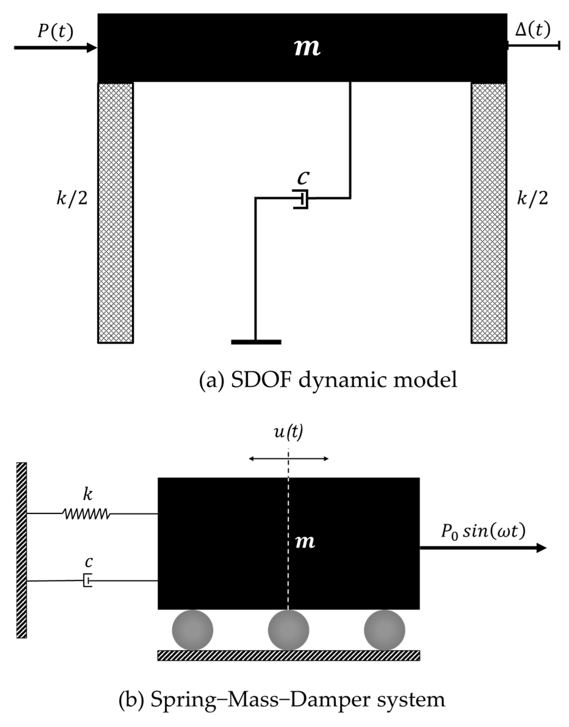
Many natural forces can be approximately represented by a series of harmonic forces, which is known as the Fourier Decomposition. A harmonic force is a simple mathematical representation of a periodic force. Figure 1 presents a spring-mass-damper system subjected to a harmonic force.

Figure 1. SDOF dynamic system subjected to a harmonic force (sinusoidally oscillating magnitude).

By examining the equation of motion for the spring-mass-damper system, its response to an external harmonic forcing function can be analyzed. This analysis reveals how the system behaves under periodic excitation, capturing both the transient response, which fades over time due to damping, and the steady-state response, which persists with characteristics dependent on the system’s parameters and the forcing frequency. The system is subjected to a sinusoidal force of the form $P_0\sin \left(\omega t\right)$, where $P_0$ represents the amplitude of the applied force, and $\omega$ denotes the angular frequency of the forcing function.

The equation of motion for the spring-mass-damper system with harmonic forcing can be expressed as

$$m\ddot{u}\left(t\right)+c\dot{u}\left(t\right)+ku\left(t\right)=P_0\sin \left(\omega t\right)$$

(1)

where $m$ represents the mass of the system, $c$ indicates the damping coefficient, $k$ is the spring constant. Moreover, $u\left(t\right)$ denotes the displacement of the mass as a function of time, $\dot{u}\left(t\right)$ and $\ddot{u}\left(t\right)$ are the first- and second-time derivatives of $u\left(t\right)$, representing velocity and acceleration, respectively.

Equation (1) represents the dynamic response of a system subjected to an external harmonic force. Its solution generally comprises two components: the transient response, which diminishes over time due to damping, and is an oscillation at the damped natural frequency $\left({\omega }_d\right)$, and the steady-state response, which remains as long as the harmonic force is applied. The steady-state solution typically follows a sinusoidal pattern with the same frequency as the forcing function but includes a phase shift and an amplitude determined by the system’s parameters and the forcing frequency $\left(\omega \right)$.

The analysis of this system is crucial in understanding phenomena such as resonance, where the amplitude of the system’s response becomes significantly large when the forcing frequency $\omega$ approaches the system’s natural frequency ${\omega }_n=\sqrt{{\displaystyle \frac{k}{m}}}$. Damping plays a critical role in limiting the amplitude of the response, especially near resonance.

The inclusion of the harmonic forcing function $P_0\sin \left(\omega t\right)$ introduces a dynamic driving mechanism that significantly influences the system’s behavior, leading to important insights into the interplay between external forces and the system’s inherent properties.

In Equation (1) $P_0\sin \left(\omega t\right)$ denotes a non-homogeneous second-order differential equation. The objective now is to solve this differential equation to derive an expression for displacement as a function of time, $u\left(t\right)$. Since this is a non-homogeneous second-order differential equation, its solution consists of two components: the complementary solution, which corresponds to the solution of the associated homogeneous equation, as presented in Equation (2), and the particular solution, which accounts for the effects of the non-homogeneous term.

$$u_c\left(t\right)=e^{-\xi {\omega }_{n}t}[A\sin \left({\omega }_{d}t\right)+B\cos \left({\omega }_{d}t\right)]$$

(2)

$$u\left(t\right)=u_c\left(t\right)+u_p(t)$$

(3)

The damping coefficient $c$ is related to the damping ratio $\xi$ through the expression $c=2m\xi {\omega }_n$, where ${\omega }_n$ is the undamped natural circular frequency of the system. Equation (3) represents the general solution of a non-homogeneous second-order differential equation describing a system’s response. It is composed of two parts: the complementary solution $u_c\left(t\right)$ and the solution $u_p\left(t\right)$. The complementary solution, $u_c\left(t\right)$, is the solution to the homogeneous equation when the external forcing term is absent and represents the system’s natural response, also known as the free vibration or transient response. This part depends on the system’s initial conditions and damping, and it gradually decays over time. The particular solution, $u_p\left(t\right)$, accounts for the effects of the external forcing function, representing the forced vibration or steady-state response, which persists as long as the external force is applied. Together, these two components fully describe the system’s displacement $u\left(t\right)$ over time, the transient response gradually diminishes, and the steady-state response determines the long-term behavior of the system under external excitation.

Given that the right-hand side of the equation is a sinusoidal function, the trial solution is chosen to be a generalized sinusoidal form, as shown in Equation (4). This assumes that the system’s response will also follow a sinusoidal pattern but with potentially different amplitude and phase. To proceed, this trial solution was differentiated, and the resulting expressions were then substituted back into the original differential equation. This substitution process is described by Equation (5), which uses the trial solution and its derivatives to determine the unknown parameters. Through this method, the specific amplitude and phase of the system’s steady-state response under the given sinusoidal forcing function were determined.

$$u_p\left(t\right)=Asin\left(\omega t\right)+Bcos\left(\omega t\right)$$

(4)

$$\left\{\begin{array}{c}{\dot{u}}_p\left(t\right)=A\omega \cos \left(\omega t\right)-B\omega \sin \left(\omega t\right)\\ {\ddot{u}}_p\left(t\right)=-A{\omega }^2\sin \left(\omega t\right)-B{\omega }^2\cos \left(\omega t\right)\end{array}\right.$$

(5)

Applying Equations (4) and (5) in Equation (1) will result in

$$\begin{gathered} m[-A{\omega }^2\sin \left(\omega t\right)-B{\omega }^2\cos \left(\omega t\right)]+c[A\omega \cos \left(\omega t\right)-B\omega \mathrm{s}\mathrm{i}\mathrm{n}(\omega t\left)\right] \\ +k[Asin\left(\omega t\right)+Bcos(\omega t\left)\right]=P_0\sin \left(\omega t\right) \end{gathered}$$

(6)

or

$$\left(k-m{\omega }^2\right)[A\sin \left(\omega t\right)+B\cos \left(\omega t\right)]+c\omega [A\cos \left(\omega t\right)-B\sin \left(\omega t\right)]=P_0\sin \left(\omega t\right)$$

(7)

Expressions for the constants A and B can be derived by grouping the sine terms, as shown in Equation (8), and the cosine terms, as shown in Equation (9). This allows us to isolate the unknown constants by equating the coefficients of the sine and cosine terms on both sides of the equation.

$$A\left(k-m{\omega }^2\right)-B\left(c\omega \right)=P_0$$

(8)

$$A\left(c\omega \right)+B\left(k-m{\omega }^2\right)=0$$

(9)

Therefore, two equations with two unknowns are obtained, and simultaneous equations can be used to solve for A and B, as shown in Equations (10) and (11).

$$A={\displaystyle \frac{k-m{\omega }^2}{{(k-m{\omega }^2)}^2+{\left(c\omega \right)}^2}} P_0$$

(10)

$$B={\displaystyle \frac{-c\omega }{{(k-m{\omega }^2)}^2+{\left(c\omega \right)}^2}}{P}_0$$

(11)

Applying the constants $A$ and $B$ in Equation (4) will result in

$$u_p\left(t\right)={\displaystyle \frac{P_0}{{(k-m{\omega }^2)}^2+{\left(c\omega \right)}^2}}[\left(k-m{\omega }^2\right)\sin \left(\omega t\right)-c\omega \cos \left(\omega t\right)]$$

(12)

Considering Equation (4) and the complementary and particular solutions, the complete expression for the response of the Single Degree of Freedom (SDOF) system under harmonic excitation is obtained as Equation (13), which includes the transient and steady-state responses.

$$u\left(t\right)=e^{-\xi {\omega }_{n}t}[A\sin \left({\omega }_{d}t\right)+B\cos ({\omega }_{d}t)]+{\displaystyle \frac{P_0}{{\left(k-m{\omega }^2\right)}^2+{\left(c\omega \right)}^2}}[\left(k-m{\omega }^2\right)\sin \left(\omega t\right)-c\omega \cos \left(\omega t\right)]$$

(13)

The dimensionless response equation offers an alternative representation of the complete response, as described in Equation (13). This formulation utilizes dimensionless ratios to simplify analysis and facilitate generalization across diverse systems. One key dimensionless parameter is the frequency ratio, denoted $\beta$, which is defined as the ratio of the excitation frequency $\omega$ to the system’s natural frequency ${\omega }_n$ expressed as Equation (14).

$$\beta ={\displaystyle \frac{\omega }{{\omega }_n}}$$

(14)

By introducing this dimensionless parameter, the response equation can be rewritten in a form that highlights the influence of excitation frequency relative to the system’s natural frequency. This approach facilitates comparisons between different systems and provides deeper insights into resonance behavior, damping effects, and the overall dynamic characteristics of the Single Degree of Freedom (SDOF) system under harmonic excitation. The steady-state response is often represented in dimensionless form. Applying the frequency ratio $\left(\beta \right)$ in Equation (12) yields

$$u_p\left(t\right)={\displaystyle \frac{P_0}{k}}\left[{\displaystyle \frac{1}{{\left(1-{\beta }^2\right)}^2+{\left(2\xi \beta \right)}^2}}\right][(1-{\beta }^2)\sin \left(\omega t\right)-2\xi \beta \cos \left(\omega t\right)]$$

(15)

Therefore, the final response equation can be restated as presented in Equation (16).

$$u\left(t\right)=e^{-\xi {\omega }_{n}t}[A\sin \left({\omega }_{d}t\right)+B\cos ({\omega }_{d}t)]+{\displaystyle \frac{P_0}{k}}\left[{\displaystyle \frac{1}{{\left(1-{\beta }^2\right)}^2+{\left(2\xi \beta \right)}^2}}\right][(1-{\beta }^2)\sin \left(\omega t\right)-2\xi \beta \cos \left(\omega t\right)]$$

(16)

2.2. Phase Angle $\left(\varphi \right)$

In the steady-state response given by Equation (15), the term ${\displaystyle \frac{P_0}{k}}\left[{\displaystyle \frac{1}{{\left(1-{\beta }^2\right)}^2+{\left(2\xi \beta \right)}^2}}\right]$ can be replaced with $\Omega$ for simplification. Additionally, the expression $(1-{\beta }^2)\sin \left(\omega t\right)$ can be designated as Component 1, while $2\xi \beta \cos \left(\omega t\right)$ is referred to as Component 2. This decomposition allows for a more straightforward interpretation of the system’s response by distinguishing between contributions from different dynamic effects. Therefore, the steady-state response includes two components. Component 1 is in phase with the applied harmonic force, while component 2 is 90 degrees out of phase.

Since $\sin \left(\omega t\right)$ appears in both the harmonic forcing function $P_0\sin \left(\omega t\right)$ and the component 1, expressed as $\Omega (1-{\beta }^2)\sin \left(\omega t\right)$, it follows that these terms share the same phase and oscillate at the same frequency. This indicates that the response component is directly influenced by $\sin \left(\omega t\right)$ remains synchronized with the external forcing function, reinforcing the system’s steady-state behavior.

Component 2 of the steady-state response arises due to the effect of damping, which influences the system’s motion by introducing a phase shift relative to the external forcing function. This component, represented by $2\xi \beta \cos \left(\omega t\right)$ accounts for energy dissipation in the system and contributes to the overall response by modifying both the amplitude and phase characteristics. 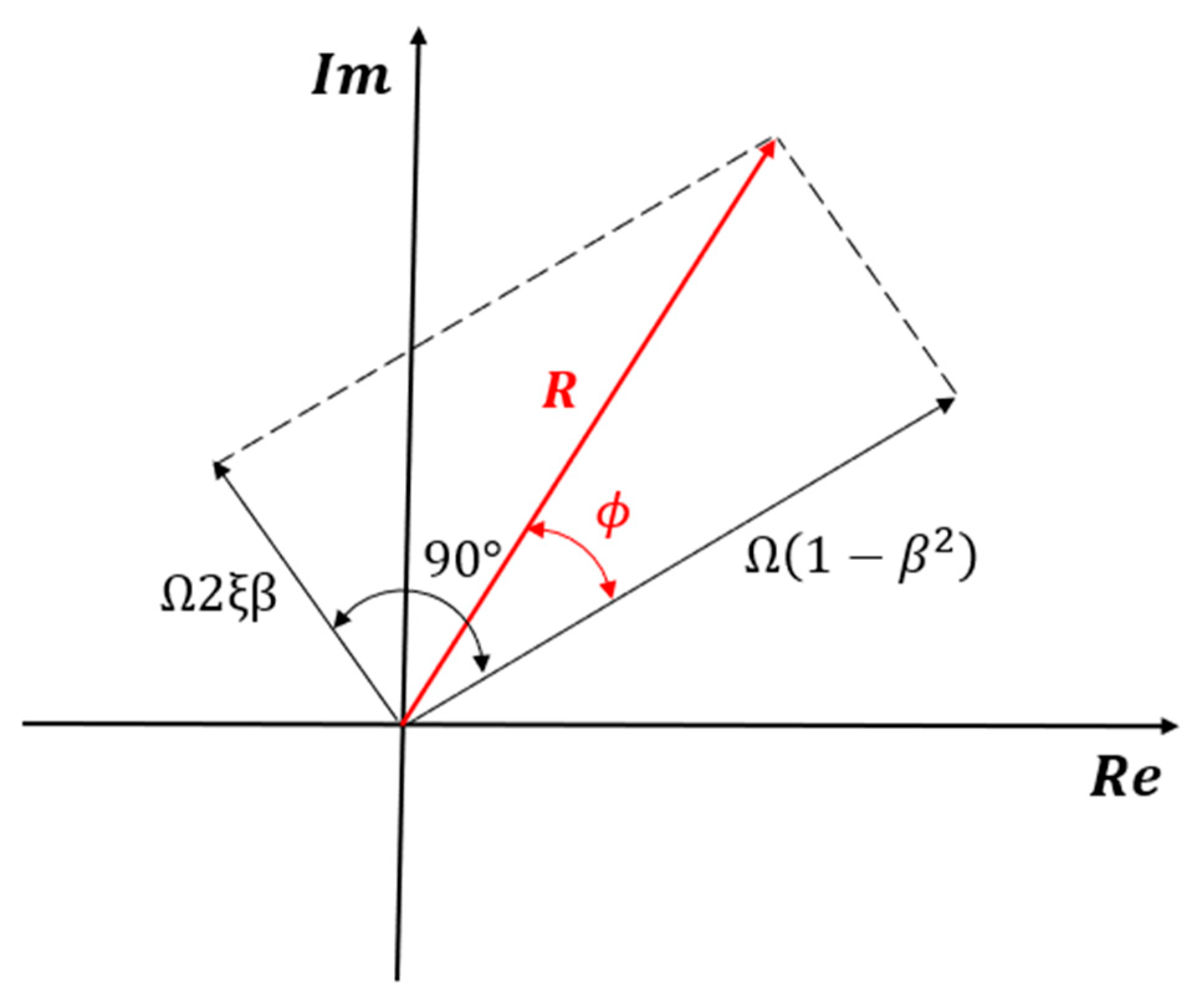The term $\cos \left(\omega t\right)$ is 90 degrees out of phase, with $\sin \left(\omega t\right)$, meaning that Components 1 and 2 are orthogonal to each other. As a result, these components can be represented as two separate vectors in a phase plane, with a 90° phase difference. This vector representation, as shown in Figure 2, facilitates a clearer understanding of how damping affects the system’s steady-state response by introducing a component that is phase-shifted relative to the external forcing function.

Figure 2. Rotating Vectors Representing Steady-State Response.

According to Figure 2, the amplitude of $R$ is the amplitude of the steady-state response. The red vector R represents the actual steady-state response and is derived as the vector sum of the two black component vectors. Its magnitude at any given moment is determined by projecting it onto the real axis.

Since the applied force is in phase with the leading response vector of magnitude $\mathrm{\Omega }(1-{\beta }^2)$, the phase angle $\varphi$ indicates how much the system’s response (red vector) lags the applied harmonic force.

As the damping level increases, the trailing vector, with a magnitude of $\mathsf{\Omega }2\mathsf{\xi }\mathsf{\beta }$, becomes longer. As a result, the overall response vector lags further behind the applied force, increasing the phase shift.

The amplitude of the steady-state response is the magnitude of the total response vector $R$, as expressed in Equation (17).

$$R=\left|u_p\left(t\right)\right|=\mathrm{\Omega }\sqrt{{(1-{\beta }^2)}^2+{\left(2\xi \beta \right)}^2}$$

(17)

Equation (17) can be restated by extending $\mathsf{\Omega }$:

$$R=\left|u_p\left(t\right)\right|={\displaystyle \frac{P_0}{k}}{\displaystyle \frac{1}{\sqrt{{(1-{\beta }^2)}^2+{\left(2\xi \beta \right)}^2}}}$$

(18)

The phase lag, denoted as $\varphi$, represents the angle between the applied force and the system’s response, as presented in Equation (19). In other words, $\varphi$ quantifies the phase shift between the external forcing function and the resulting motion of the system. This phase difference arises from damping and system dynamics, which affect how the response lags behind the applied force. A higher damping ratio increases the phase lag, meaning the system takes longer to reach its peak displacement relative to the driving force. Therefore, the steady-state response lags the applied harmonic force by phase angle $\varphi$.

$$\varphi ={\tan }^{-1}({\displaystyle \frac{2\xi \beta }{1-{\beta }^2}})$$

(19)

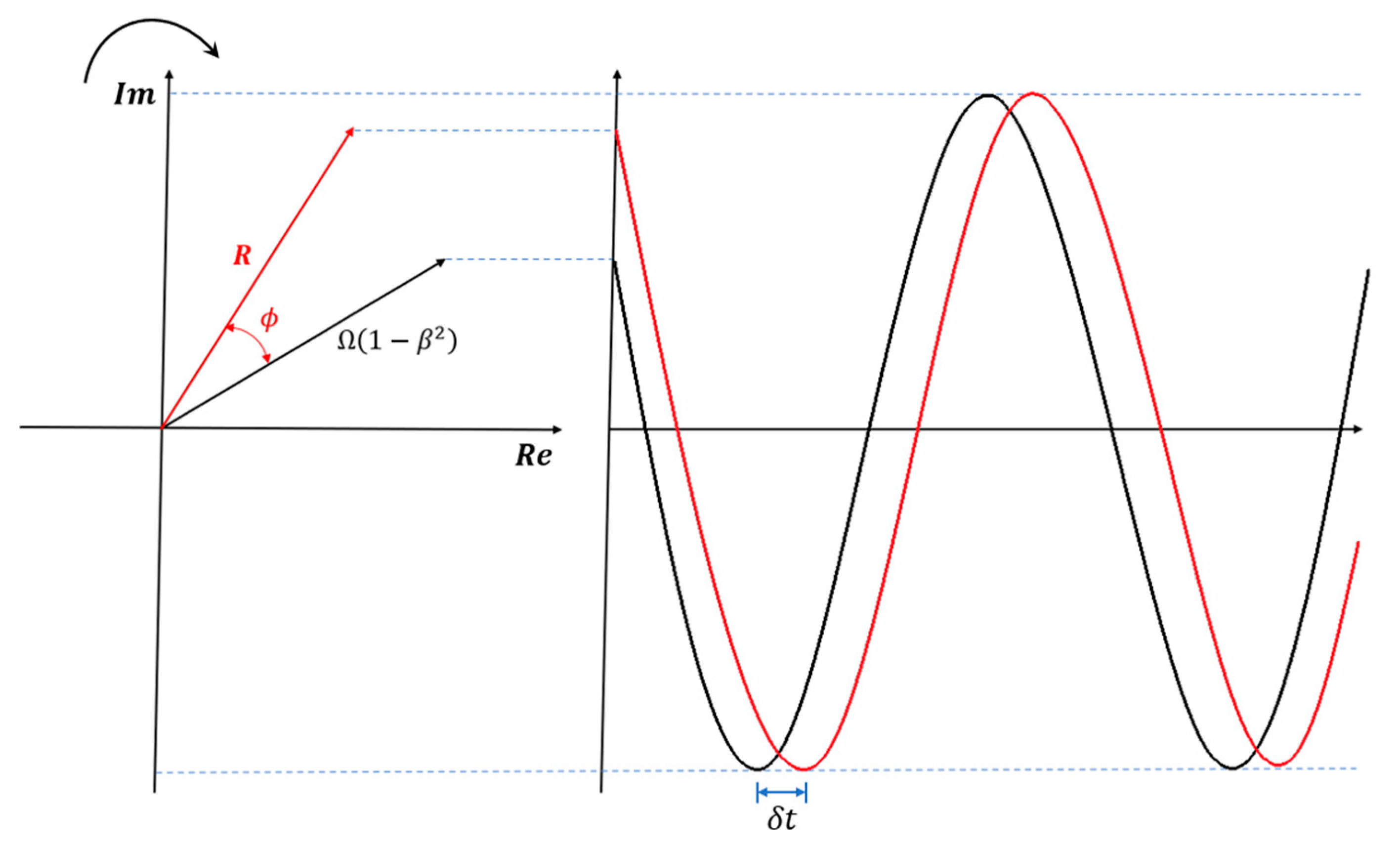
The black line in Figure 3 illustrates the waveform representing the frequency and phase of the applied force, $\sin \left(\omega t\right)$, and the red graph presents the corresponding waveform showing the phase lag of $\varphi$ degrees between the force and the system’s response, $\sin (\omega t+\varphi )$. By understanding the nature of the applied force or the specific harmonic force acting on the system, the steady-state response can be fully characterized, including the frequency and phase relationships between the applied force and the resulting motion. This allows for a comprehensive understanding of how the system behaves under harmonic excitation.

Figure 3. Phase lag between the applied harmonic force and the steady-state response.

2.3. Dynamic Magnification Factor (DMF) and Resonance

The Dynamic Magnification Factor (DMF) is a crucial parameter in structural dynamics, defined as the ratio between the amplitude of the steady-state dynamic response and the deflection caused by a static load of the same magnitude. This factor serves as a powerful tool for assessing the extent to which dynamic loading amplifies a structure’s response compared to its static counterpart. It provides engineers with insights into the influence of oscillatory forces, helping them predict potential resonance effects and ensure the structural integrity and serviceability of engineering systems. Mathematically, it is expressed as

$$DMF={\displaystyle \frac{Amplitude of Steady-State Dynamics Response}{Static Deflection Under the Same Load}}$$

(20)

Considering Equations (18) and (20), the DMF can be stated as:

$$DMF={\displaystyle \frac{\left|u\left(t\right)\right|}{\frac{P_0}{k}}}={\displaystyle \frac{1}{\sqrt{{(1-{\beta }^2)}^2+{\left(2\xi \beta \right)}^2}}}$$

(21)

The DMF and the phase angle $\varphi$ are key parameters that define the behavior of a structure or mechanical system under harmonic excitation. Both depend on the forcing frequency $(\beta ={\displaystyle \frac{\omega }{{\omega }_n}})$, the system’s natural frequency $\left({\omega }_n\right)$, and the level of damping $(\xi ={\displaystyle \frac{c}{c_{cr}}})$. The DMF quantifies the amplification of displacement caused by dynamic effects, indicating how much a harmonic force magnifies the structural response beyond its static deflection. The phase angle $\varphi$ represents the lag between the applied force and the system’s response. Together, these parameters fully characterize the steady-state response when the harmonic excitation’s frequency and amplitude are known.

Resonance occurs when a system is subjected to a periodic force whose frequency matches its natural frequency, leading to a significant increase in vibration amplitude. This occurs because the external force continuously supplies energy in sync with the system’s natural oscillations, leading to a buildup of motion that can cause structural damage or failure if not adequately controlled.

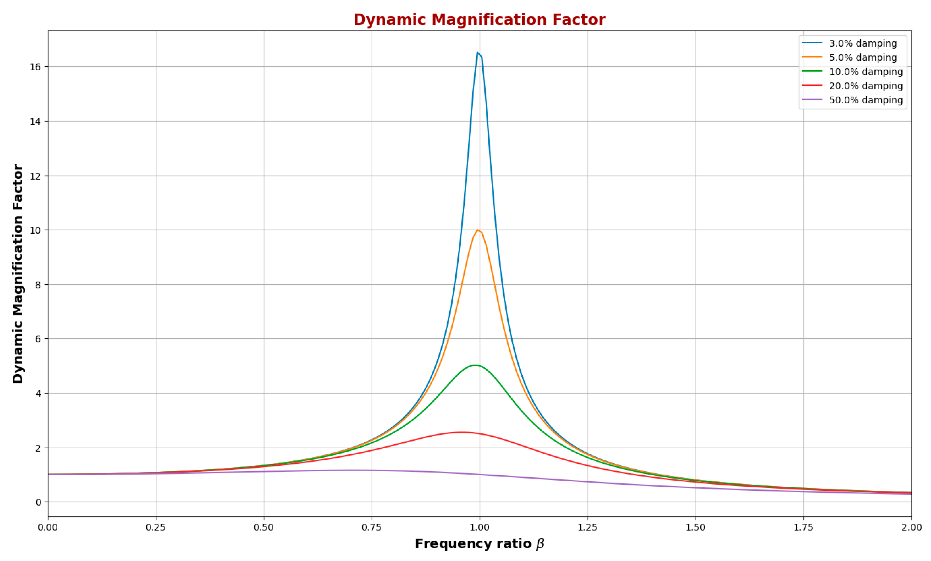
Figure 4 depicts the relationship between the frequency ratio (β) and the dynamic magnification factor (DMF) for various damping levels, ranging from 3% to 50%. The x-axis represents the frequency ratio β (dimensionless), while the y-axis shows the DMF (dimensionless).

Figure 4. Variation in Dynamic Magnification Factor (DMF) (ξ = 0.03–0.50, $m=\mathrm{15,000}$ kg, $k=\mathrm{285,714.28} \mathrm{N}$/m, $\beta grid\in [0.0, 2.0]$ with increment $\mathsf{\Delta }\beta =0.01$).

The graph demonstrates the typical behavior of a damped system under harmonic excitation. As the frequency ratio approaches 1 (resonance), the DMF increases sharply, reaching its maximum value. This peak indicates the resonance condition, where the system experiences maximum oscillation amplitude relative to the applied force.

For lower damping values, particularly 3% (blue curve) and 5% (orange curve), the peak is significantly higher, exceeding 16, and the curve exhibits a pronounced sharpness around β = 1. This sharp peak reflects the high amplification of oscillations at resonance when damping is low. As damping increases, the peak value decreases, and the curve flattens. For 10% damping (green curve), the peak is noticeably lower, reaching just over 10, and the response becomes less sensitive to frequency variations around resonance. With 20% damping (red curve) and 50% damping (purple curve), the peak continues to diminish, and the DMF approaches a more moderate level across the frequency range, illustrating a significant reduction in amplitude amplification as damping increases.

This trend highlights the role of damping in mitigating the system’s resonant response. High damping reduces the amplitude of oscillations at resonance and broadens the range of frequencies over which the system experiences lower amplification. Therefore, systems with higher damping coefficients are less likely to experience excessive oscillations or damage due to resonance, making damping an essential design factor for structures subjected to dynamic loads.

The DMF helps quantify this effect by indicating how much the system’s response is amplified under dynamic loading. As the excitation frequency approaches the natural frequency, the DMF reaches its maximum, highlighting the risk of excessive displacement. Additionally, the phase angle $\varphi$ shifts noticeably, moving from an in-phase response at low frequencies to an out-of-phase response at higher frequencies.

Understanding the relationship between the DMF, phase angle, and system parameters provides critical insights into resonance, energy dissipation, and overall vibratory behavior. As the forcing frequency approaches the natural frequency, the DMF reaches its peak, leading to maximum displacement, while the phase angle shifts from in-phase behavior at low frequencies to out-of-phase behavior at higher frequencies. By quantifying dynamic amplification, the DMF enables engineers to assess the effects of dynamic loading and anticipate potential resonance issues. To mitigate excessive vibrations and minimize resonance risks, structural design strategies can incorporate damping mechanisms, modify system stiffness, or adjust excitation conditions to achieve optimal performance.

While Eurocode 8 defines seismic design spectra for transient ground motions, the present study adopts a linear single-degree-of-freedom (SDOF) system under harmonic excitation as a conceptual and computational benchmark. This simplification enables systematic validation of the proposed hybrid PINN–EKF framework under well-controlled dynamic conditions, where the analytical solution is known and the effects of parameter uncertainty and noise can be rigorously assessed. The insights gained from this harmonic analysis provide a foundational step toward extending the method to nonlinear and multi-degree-of-freedom (MDOF) systems driven by recorded or spectrum-compatible seismic excitations, thereby supporting future code calibration and performance-based design developments.

3. Conventional Numerical Analysis of Structural Dynamics

In this section, structural dynamic principles are applied to analyze the response of a lightweight steel frame supporting heavy machinery with a total mass of m = 15,000 kg, assuming the frame’s self-weight is negligible. An experimental impact test estimates the inherent structural damping as ξ = 0.03. The structure is laterally constrained, preventing twisting and significant vertical movement, allowing it to be modeled as a single-degree-of-freedom (SDOF) system under harmonic excitation. A load test reveals that a lateral force of P = 2000 N results in a lateral displacement of Δ = 7 mm. Given a harmonic force of magnitude P₀ = 700 N and a forcing frequency of f = 0.9 Hz, the dynamic magnification factor and the phase shift between the applied force and steady-state response were determined. Additionally, the structural response over t ∈ [0, 60] s was analyzed, and if the harmonic force is removed at t = 10 s, the mass position at t = 45 s was determined.

In the next section, machine learning and optimization algorithms are introduced to predict and refine the system’s hyperparameters, and their performance is compared with the structural dynamic approach to evaluate their effectiveness in analyzing and optimizing the structural response.

3.1. DMF and Phase Shift $\varphi$

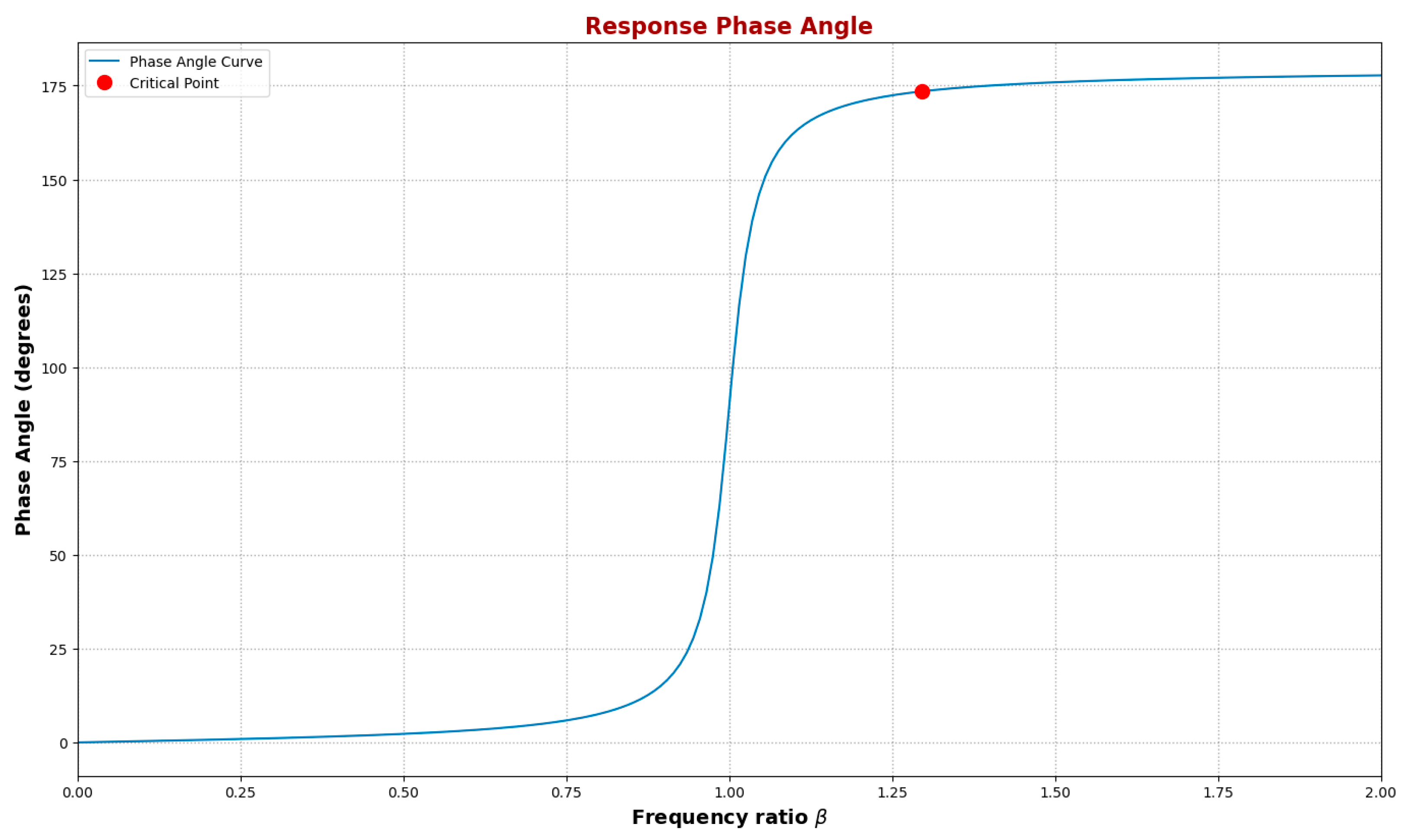
Figure 5 is presented by applying Equation (21) for the dynamic magnification factor (DMF) and Equation (19) for the phase shift $\left(\varphi \right)$ between the applied force and the system’s response.

Figure 5. Phase Angle Response of the Damped SDOF System under Harmonic Excitation ($m=\mathrm{15,000} \mathrm{kg}$, $k=\mathrm{285,714.28} \mathrm{N}/\mathrm{m}$, $\xi =0.03$, $P_0=700 \mathrm{N}$, $\beta grid\in [0.0,2.0]$ with Δβ = 0.01).

Figure 5 illustrates the Response Phase Angle as a function of the frequency ratio (β) in a harmonically excited SDOF system, where the phase angle represents the lag between the applied force and the system’s response. It illustrates the expected phase behavior of a damped SDOF system under harmonic excitation, with a key characteristic being the transition from in-phase to out-of-phase response. Beyond the resonance region, the system’s response significantly lags the excitation.

At low-frequency ratios (β < 1.0), the phase angle remains close to 0°, indicating that the system’s response is nearly in phase with the applied force. As the frequency ratio approaches β = 1.0, a rapid transition occurs, marking the onset of the resonance region. In this range, the phase angle shifts dramatically from near 0° to 180°, indicating that the system transitions from being in phase with the applied force to almost entirely out of phase.

Beyond the resonance region (β > 1.0), the phase angle stabilizes at approximately 180°, indicating that the response consistently lags the applied force by half a cycle. The critical point, marked at β ≈ 1.296, highlights a phase difference of approximately 173.5° (3.028 radians), corresponding to a dynamic magnification factor (DMF) of 1.463 and a steady-state dynamic amplitude of 0.0036 m. The static deflection, obtained by dividing the force magnitude by the stiffness, is 0.0025 m. Table 1 summarizes the results presented above for the damped SDOF system.

Table 1. Phase Angle and Dynamic Response of the Damped SDOF System.

Frequency Ratio (β)	Phase Angle (°)	Dynamic Magnification Factor (DMF)	Steady-State Dynamic Amplitude (m)	Static Deflection (m)	Remarks
β < 1.0	~0°	-	-	-	The response is nearly in phase with the force.
β ≈ 1.0	Rapid transition	-	-	-	Resonance region, phase shifts from 0° to 180°.
β > 1.0	~180°	-	-	-	Response lags force by half a cycle.
β ≈ 1.296	173.5° (3.028 radians)	1.463	0.0036	0.0025	Post-resonance response lags excitation.

3.2. Structural Response

Equation (16) was used to calculate the system’s response to the harmonic loading. Therefore, the constants $A$ and $B$ within the transient component must first be determined. This is achieved by applying the initial conditions. At $t=0$, both the position $u(t=0)$ and velocity $\dot{u}(t=0)$ are zero. To apply the second boundary condition on velocity, the expression for $u\left(t\right)$ must first be differentiated. For simplicity, some substitutions will be made to make the equation more manageable.

As mentioned in Section 2.2

$$\mathrm{\Omega }={\displaystyle \frac{P_0}{k}}\left[{\displaystyle \frac{1}{{(1-{\beta }^2)}^2+{\left(2\xi \beta \right)}^2}}\right]$$

(22)

$$\left\{\begin{array}{c}{C}_1=\Omega (1-{\beta }^2)\\ C_2=-\Omega 2\xi \beta \end{array}\right.$$

(23)

Applying Equations (22) and (23), Equation (16) was restated as follows:

$$\begin{gathered} u\left(t\right)=A\left[e^{-\xi {\omega }_{n}t}\sin \left({\omega }_{d}t\right)\right]+B\left[e^{-\xi {\omega }_{n}t}\cos \left({\omega }_{d}t\right)\right] \\ +C_1\sin \left(\omega t\right)+C_2\cos \left(\omega t\right) \end{gathered}$$

(24)

Considering the following assumptions

$$\left\{\begin{array}{c}{f}_1\left(t\right)=\left[e^{-\xi {\omega }_{n}t}\sin \left({\omega }_{d}t\right)\right]\\ f_2\left(t\right)=\left[e^{-\xi {\omega }_{n}t}\cos \left({\omega }_{d}t\right)\right]\\ f_3\left(t\right)=\sin \left(\omega t\right)\\ f_4\left(t\right)=\cos \left(\omega t\right)\end{array}\right.$$

(25)

while

$$u\left(t\right)=A{f}_1\left(t\right)+B{f}_2\left(t\right)+C_1{f}_3\left(t\right)+C_2{f}_4\left(t\right)$$

(26)

Each of the four functions of $t$ can be differentiated individually. The functions $f_1\left(t\right)$ and $f_2\left(t\right)$ can be differentiated using the product rule, while $f_3\left(t\right)$ and $f_4\left(t\right)$ can be differentiated using the chain rule. Therefore

$${\displaystyle \frac{d}{dt}}{f}_1\left(t\right)=e^{-\xi {\omega }_{n}t}{\omega }_d\cos \left({\omega }_{d}t\right)-\sin \left({\omega }_{d}t\right)\xi {\omega }_n{e}^{-\xi {\omega }_{n}t}$$

(27)

$${\displaystyle \frac{d}{dt}}{f}_2\left(t\right)=-e^{-\xi {\omega }_{n}t}{\omega }_d\sin \left({\omega }_{d}t\right)-\cos \left({\omega }_{d}t\right)\xi {\omega }_n{e}^{-\xi {\omega }_{n}t}$$

(28)

$${\displaystyle \frac{d}{dt}}{f}_3\left(t\right)=\omega \cos \left(\omega t\right)$$

(29)

$${\displaystyle \frac{d}{dt}}{f}_4\left(t\right)=-\omega \sin \left(\omega t\right)$$

(30)

Therefore, the velocity $\dot{u}\left(t\right)$ can be formulated as presented in Equation (31).

$$\dot{u}\left(t\right)=A\left[e^{-\xi {\omega }_{n}t}{\omega }_d\cos \left({\omega }_{d}t\right)-\sin \left({\omega }_{d}t\right)\xi {\omega }_n{e}^{-\xi {\omega }_{n}t}\right]+B\left[-e^{-\xi {\omega }_{n}t}{\omega }_d\sin \left({\omega }_{d}t\right)-\cos \left({\omega }_{d}t\right)\xi {\omega }_n{e}^{-\xi {\omega }_{n}t}\right]+C_1\omega \cos \left(\omega t\right)-C_2\omega \sin \left(\omega t\right)$$

(31)

Considering the equations of $u\left(t\right)$ and $\dot{u}\left(t\right)$, and applying the initial condition $t=0$, the unknown hyperparameters will be

$$A=-{\displaystyle \frac{1}{{\omega }_d}}(C_1\omega +C_2\xi {\omega }_n)$$

(32)

$$B=-C_2$$

(33)

As shown in Figure 6, the transient response gradually diminishes over time due to damping, allowing the system’s behavior to be effectively characterized by the steady-state response. Once the transient effects dissipate, the system stabilizes into periodic oscillations dictated by its natural frequency and external forcing, making the steady-state response the primary focus for analysis and practical applications.

Figure 6. Components of Displacement-Time History: Transient and Steady-State Responses.

The displacement-time history in the figure captures both transient and steady-state components. Initially, the transient response exhibits oscillations with an amplitude of approximately ±0.004 m, which progressively decay as energy dissipates. By t ≈ 20 s, the transient effects become negligible, and the system transitions into steady-state behavior.

In this steady-state phase, the displacement oscillates with a nearly constant amplitude of about ±0.0025 m, following a sinusoidal pattern. The static displacement, representing the equilibrium position, is also plotted, along with the steady-state amplitude, which marks the stabilization of oscillations.

This response confirms that after an initial disturbance, the system undergoes damped oscillatory motion before settling into a stable vibration pattern. The well-defined steady-state oscillations and the decay of the transient component align with theoretical expectations, illustrating the balance between external forcing and damping.

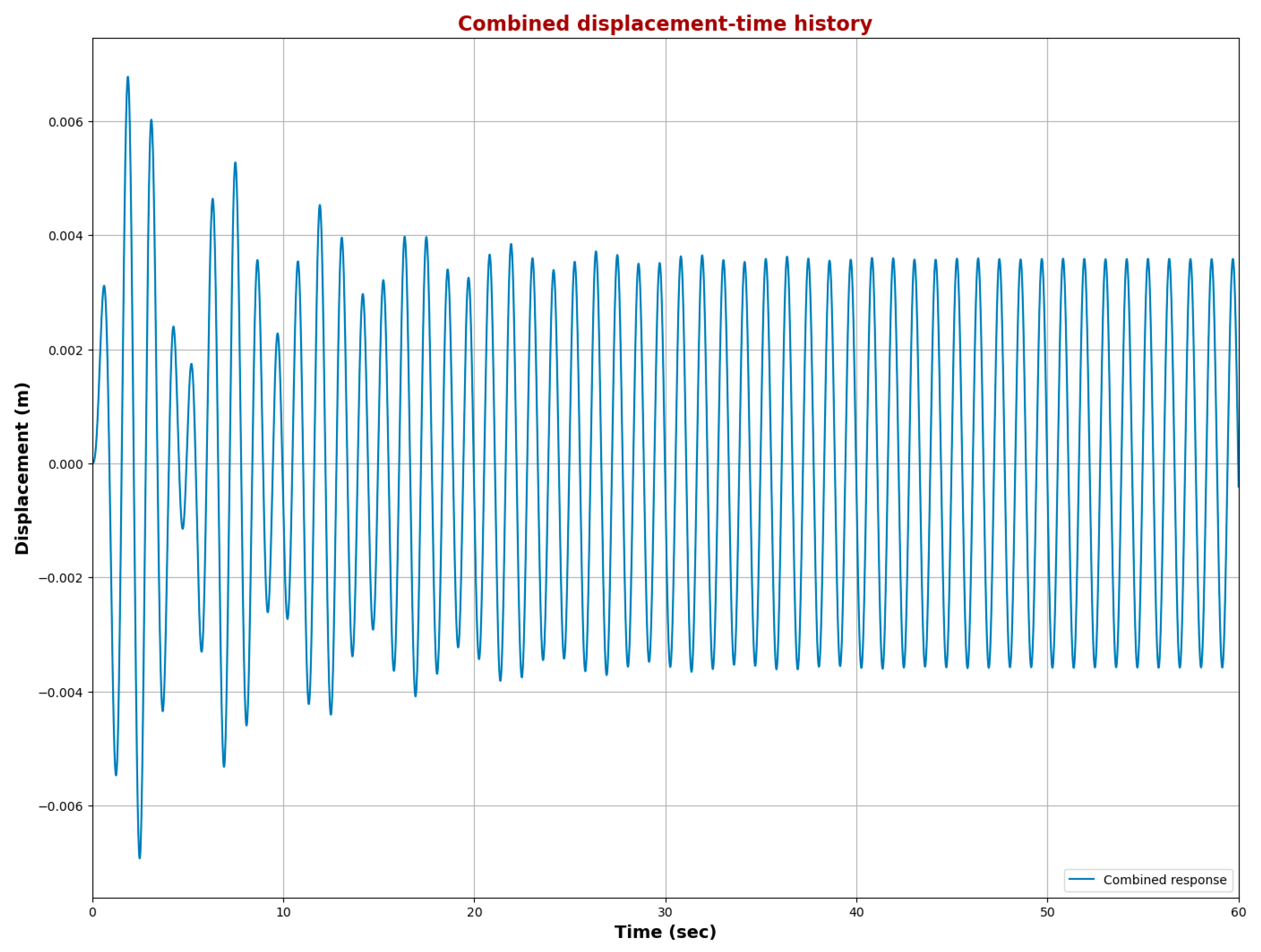
Figure 7 illustrates the combined displacement-time history of a dynamic system, capturing both the transient and steady-state responses. Initially, the displacement exhibits high-amplitude oscillations, reaching approximately ±0.0065 m, which gradually diminish over time due to damping. This transient phase, evident in the first 20 s, is characterized by a reduction in oscillation magnitude as energy dissipates from the system.

Figure 7. Displacement-Time History: Transient and Steady-State Response.

Beyond t ≈ 20 s, the transient response becomes negligible, and the system settles into a periodic steady-state oscillation. In this phase, the displacement stabilizes within a consistent amplitude range of approximately ±0.0025 m. The oscillatory pattern in the steady-state response aligns with the system’s natural frequency and the influence of external excitation forces.

The observed behavior aligns with theoretical expectations: an initial disturbance triggers a damped transient response, followed by a steady-state vibration governed by the balance between external forcing and damping. The results confirm that after an initial phase of energy dissipation, the system exhibits predictable harmonic motion with a stable amplitude, making the steady-state response the primary focus for long-term analysis.

3.3. Free Vibration Response

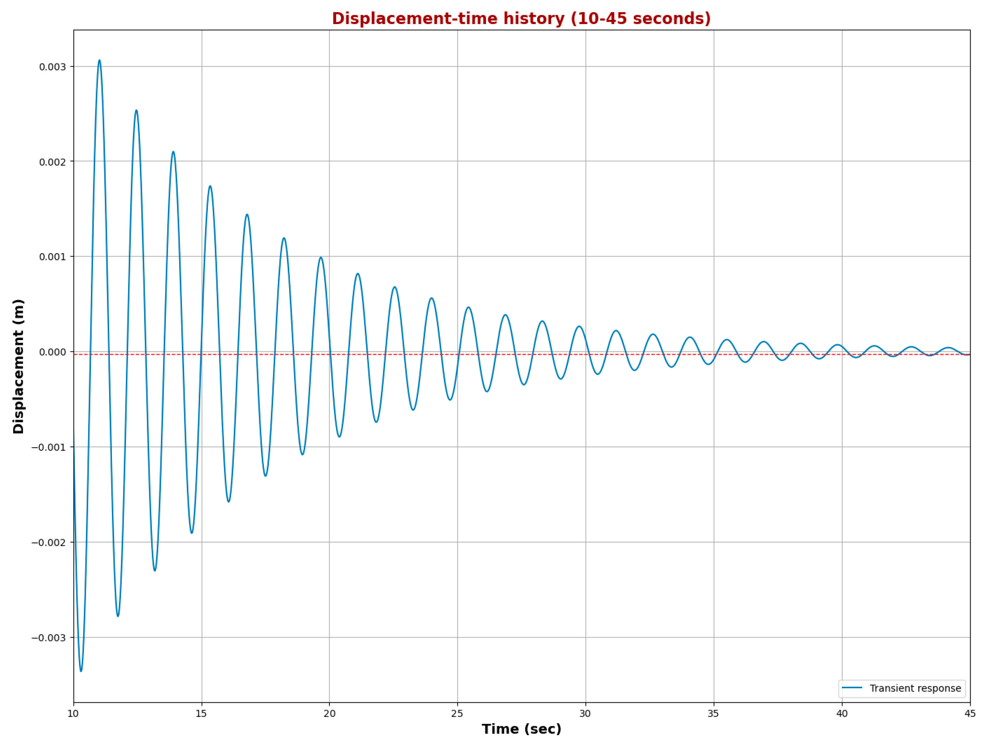
The harmonic excitation is removed at t = 10 s, leading to a change in the system’s dynamic response. Initially, the system exhibits forced vibration behavior due to the applied harmonic force, characterized by oscillations influenced by both transient and steady-state responses. Once the external force is removed, the system transitions into free vibration, where its natural frequency and damping characteristics govern its motion.

To determine the position of the mass at t = 45 s, the displacement function should be analyzed with respect to the governing differential equation of motion. Before the force is removed, the displacement follows a combination of transient and steady-state oscillations. After t = 10 s, the system undergoes damped free vibration, during which the displacement gradually diminishes due to damping. By evaluating the displacement function at t = 45 s, the precise position of the mass can be determined, reflecting the long-term behavior of the system in the absence of external excitation. The numerical result for the displacement at this instant would depend on the system parameters, including mass, damping coefficient, and natural frequency.

The displacement and velocity values obtained in the previous step now serve as the initial conditions for determining the free vibration response at t = 45 s. At this point, our focus shifts solely to the system’s transient response. It is no longer a concern with steady-state conditions but instead with how the system behaves over time, starting from the new initial conditions.

$$u\left(t\right)=e^{-\xi {\omega }_{n}t}[A\sin \left({\omega }_{d}t\right)+B\cos \left({\omega }_{d}t\right)]$$

(34)

To proceed, it is necessary to determine the constants $A$ and $B$ that characterize the system’s transient response. These constants depend on the initial displacement and velocity, which have been established in the previous step. As a result, the general expressions for displacement and velocity were restated, incorporating the new initial conditions, to solve for $A$ and $B$. By doing so, we will be able to fully characterize the system’s motion at any given time, particularly during the transient phase, and gain insights into its dynamic behavior at t = 45 s. By calculating and applying the boundary conditions $u(t=10)=-0.0007\hspace{0.17em}\mathrm{m}$ and $\dot{u}(t=10)=-0.0148\hspace{0.17em}$ m/s to both expressions, we obtain two simultaneous equations.

$$u\left(t\right)=A\left[e^{-\xi {\omega }_{n}t}\sin \left({\omega }_{d}t\right)\right]+B\left[e^{-\xi {\omega }_{n}t}\cos \left({\omega }_{d}t\right)\right]$$

(35)

$$\dot{u}\left(t\right)=A\left[e^{-\xi {\omega }_{n}t}{\omega }_d\cos \left({\omega }_{d}t\right)-\sin \left({\omega }_{d}t\right)\xi {\omega }_n{e}^{-\xi {\omega }_{n}t}\right]+B\left[-e^{-\xi {\omega }_{n}t}{\omega }_d\sin \left({\omega }_{d}t\right)-\cos \left({\omega }_{d}t\right)\xi {\omega }_n{e}^{-\xi {\omega }_{n}t}\right]$$

(36)

Expressing the results in matrix form yields

$$\left[\begin{array}{cc}-0.0956& 0.2525\\ 1.114& 0.384\end{array}\right]\times \left[\begin{array}{c}A\\ B\end{array}\right]=\left[\begin{array}{c}-0.0007\\ -0.0148\end{array}\right]$$

(37)

Solving Equation (37), we obtain $A=-0.011$ and $B=-0.007$. By calculating the equations for free vibration at $t=45$ s, the response magnitude is $-0.00003$ m, as presented by the red line in Figure 8.

Figure 8. Transient Displacement Response of the System (10–45 s).

Figure 8 shows the displacement-time history of the system from 10 to 45 s, illustrating its transient response. The displacement is plotted on the vertical axis in meters, while time is represented on the horizontal axis in seconds. The system undergoes oscillations with progressively decreasing amplitude, indicating the damping effect over time. Initially, there is a significant peak around 10 s, where the displacement reaches approximately 0.003 m. The displacement then decreases with each subsequent peak and trough, showing an oscillatory pattern. By the end of the graph at 45 s, the oscillations have nearly damped out, and the displacement approaches zero, indicating that the system has stabilized. According to the analysis above, the displacement response at t = 45 s is −0.00003 m. This final displacement value is indicated by the red line in the graph, which shows the system’s near-zero displacement at this time, confirming that the system’s oscillations have significantly damped and that the transient phase has ended.

4. Data Assimilation Model for Fitting Displacement Curves

In the preceding analyses, the numerical solution of the single-degree-of-freedom (SDOF) harmonically excited system was obtained under the ideal assumption that all model parameters were known exactly. In real-world engineering, however, many of these parameters—such as mass, damping coefficient, stiffness, excitation amplitude, and frequency—must be estimated through measurements, which are inherently prone to noise and uncertainty. These discrepancies between measured and actual values result in deviations in the predicted displacement-time response from the ideal numerical solution. The closer the estimated parameters are to their exact values, the more accurately the system’s dynamic behavior can be reproduced, making parameter estimation a critical task in engineering applications.

Despite the existence of an analytical solution to the linear second-order vibration equation $m\ddot{u}\left(t\right)+c\dot{u}\left(t\right)+ku\left(t\right)=P_0\sin \omega t$, its direct application in practice often encounters several challenges:

Parameter Uncertainty: Real-world parameters vary due to manufacturing tolerances, aging, and environmental effects, which reduces the reliability of purely analytical predictions.

• Sensitivity to Initial Conditions: Analytical solutions are highly dependent on accurate initial conditions, which are challenging to measure precisely in practice.
• Measurement Noise and Sparse Sampling: Observational data are typically noisy and collected at discrete intervals, limiting the resolution and reliability of direct comparisons with model predictions.
• Model Idealization Bias: Simplified models often overlook complex behaviors, such as nonlinear damping and stochastic external forces, thereby failing to capture the full dynamics of real structures.

To overcome these limitations, data assimilation techniques, such as the Extended Kalman Filter (EKF), are employed. These methods integrate numerical models with observational data, correcting predictions by accounting for parameter uncertainties and measurement errors. EKF enhances system identification by providing real-time updates, quantifying estimation uncertainty, and improving the accuracy and robustness of vibration monitoring and control systems. Even when analytical solutions are available, data assimilation remains a vital tool due to its adaptability and reliability in complex, uncertain environments.

4.1. The EKF Method

The Extended Kalman Filter (EKF) is an extension of the classical Kalman Filter (KF), specifically designed to address the state estimation problem in non-linear systems. While the standard Kalman Filter is limited to linear Gaussian systems, real-world engineering systems often exhibit nonlinear behaviors, rendering the direct application of the classical KF invalid.

The core idea of the EKF is to preserve the recursive structure of the Kalman Filter by locally linearizing the nonlinear system. This is achieved by performing a first-order Taylor expansion of the non-linear state and observation functions around the current state estimate, thereby neglecting higher-order terms. The partial derivatives of these non-linear functions with respect to the state variables form the Jacobian matrices, which serve as linear approximations of the system dynamics and observation models.

In the EKF framework, both the state transition and observation equations are linearized independently. The estimation process consists of two sequential steps. In the prediction step, the algorithm uses the system model and the previous state estimate to forecast the current state and its associated covariance. This predicted state is then refined in the update step, where actual observational data are incorporated to correct the prediction, yielding an improved, more accurate state estimate.

Through this approach, the EKF effectively extends the applicability of Kalman filtering to a broad class of non-linear dynamic systems, enabling more accurate and robust estimation under realistic conditions. The general non-linear system governed by the following state and observation equations is considered:

$$\left\{\begin{array}{c}{x}_k=f\left(x_{k-1},u_{k-1}\right)+w_{k-1}\\ z_k=h\left(x_{k-1}\right)+v_k\end{array}\right.$$

(38)

where

$x_k\in {\mathbb{R}}^n$ is the state vector at the moment $k$

$u_k\in {\mathbb{R}}^m$ presents the control input at the moment $k$

$z_k\in {\mathbb{R}}^p$ denotes the observation vector at the moment $k$

$f\left(\cdot \right)$ stands for the non-linear state transfer function

$h\left(\cdot \right)$ shows the non-linear observation function

$w_k~\mathcal{N}(0,Q_k)$ is the process noise with a covariance matrix $Q_k$

$v_k~\mathcal{N}(0,R_k)$ illustrates the observation noise with a covariance matrix $R_k$

The core idea of the EKF is to linearize the nonlinear system using a Taylor expansion and then apply the prediction and update steps of Kalman filtering. The basic process of extended Kalman filtering can be summarized as follows:

Initialize the state and covariance:

$$\left\{\begin{array}{c}{\widehat{x}}_{0|0}=x_0\\ P_{0|0}=P_0\end{array}\right.$$

(39)

where ${\widehat{x}}_{0|0}$ is the initial state estimate and $P_{0|0}$ presents the initial state covariance matrix. At each time step, the prediction step (state prediction and covariance prediction) is performed first, as presented in Equations (40) and (41).

$${\widehat{x}}_{k|k-1}=f({\widehat{x}}_{k-1|k-1},u_{k-1})$$

(40)

$$P_{k|k-1}=F_k{P}_{k-1|k-1}{F}_k^T+Q_{k-1}$$

(41)

where

${\widehat{x}}_{k|k-1}$ is the a priori state estimate at moment $k$

$P_{k-1|k-1}$ shows the a priori covariance matrix

$F_k$ is the Jacobi matrix of the state transfer function $f(\cdot )$ at $x={\widehat{x}}_{k-1|k-1}$

$$F_k={{\displaystyle \frac{\partial f}{\partial x}}|}_{x={\widehat{x}}_{k-1|k-1}}$$

(42)

According to Equations (43)–(45), the update step (correcting the state estimates and covariances using the observed data) is then performed.

$$K_k=P_{k|k-1}{H}_k^T{({H_{k}P}_{k|k-1}{H}_k^T+R_k)}^{-1}$$

(43)

$${\widehat{x}}_{k|k}={\widehat{x}}_{k|k-1}+K_k(z_k-h({\widehat{x}}_{k|k-1}\left)\right)$$

(44)

$$P_{k|k}=(I-K_k{H}_k)P_{k|k-1}$$

(45)

where

$K_k$ denotes the Kalman gain

${\widehat{x}}_{k|k}$ is the a posteriori state estimate at moment $k$

$P_{k|k}$ represents the a posteriori covariance matrix

$H_k$ shows the Jacobian matrix of the observation function $h\left(\cdot \right)$ at ${\widehat{x}}_{k|k-1}$

$$H_k={{\displaystyle \frac{\partial h}{\partial x}}|}_{x={\widehat{x}}_{k|k-1}}$$

(46)

For this case, we treat the parameters θ = {c, P₀, ω} as fixed known quantities (c, P₀, ω are used directly in the system). This means that the EKF only estimates the state vector $\mathit{x}=[u,\hspace{0.25em}v{]}^{\top }$. The observed displacement $z=u$ corresponds to the observation matrix $H=\left[1 0\right]$. The vector form of the continuous-time state equation is

$$\dot{\mathit{x}}=f\left(\mathit{x},t\right)=\left[\begin{array}{c}v\\ {\displaystyle \frac{P_0\mathit{sin}\left(\omega t\right)-cv-ku}{m}}\end{array}\right]$$

(47)

While the state Jacobian is stated as

$$F_c={\displaystyle \frac{\partial f}{\partial x}}=\left[\begin{array}{cc}0& 1\\ -{\displaystyle \frac{k}{m}}& -{\displaystyle \frac{c}{m}}\end{array}\right]$$

(48)

The discretization is approximated by $\mathit{\Phi }\approx I+F_c\mathit{\Delta }t$.

In this experiment, the initial state is ${\mathit{x}}_{0\mid 0}=[0.1,\hspace{0.25em}0.0{]}^{\top }$, the initial covariance is considered as $P_{0\mid 0}=diag\left(0.1,\hspace{0.25em}0.1\right)$, the process noise is set to $Q=diag\left(1\times {10}^{-3},\hspace{0.25em}1\times {10}^{-3}\right)$, and the observation noise variance is $R={\sigma }_{obs}^2=1\times {10}^{-6}$.

While the EKF extends the classical Kalman framework to nonlinear systems, its performance relies on several assumptions that may limit its applicability in complex structural dynamics problems. The EKF linearizes the nonlinear state-transition and observation models using a first-order Taylor expansion, which can introduce approximation errors when the system exhibits strong nonlinearities, such as yielding, hysteretic damping, or stiffness degradation. Moreover, EKF assumes that both process and measurement noise follow zero-mean Gaussian distributions with known covariances. In practice, seismic or experimental data often include non-Gaussian noise, bias, or outliers, which can degrade estimation accuracy or lead to divergence. Under such conditions, alternatives such as the Unscented Kalman Filter (UKF), Ensemble Kalman Filter (EnKF), or Particle Filter (PF) may offer improved robustness. In this study, the EKF is primarily applied to moderately nonlinear, single-degree-of-freedom systems where linearization remains valid. To further mitigate these limitations, the complementary use of the Physics-Informed Neural Network (PINN) enhances stability and accuracy under noisy or partially nonlinear conditions, providing a balanced hybrid estimation framework.

4.2. Numerical Experiment

The numerical experiments are based on the hypotheses developed in Section 3, as summarized in Table 2.

Table 2. Model Parameters and Assumptions for Numerical Experiments.

Parameter	Description	Value
Structure Type	Lightweight steel frame supporting heavy machinery	—
Total Mass (m)	Mass of machinery (frame’s self-weight neglected)	15,000 kg
Damping Ratio (ξ)	Estimated inherent structural damping from the impact test	0.03
Boundary Condition	Laterally constrained	—
Model Type	SDOF system under harmonic excitation	—
Static Lateral Force (P)	Force applied in the static load test	2000 N
Static Lateral Displacement (Δ)	Resulting in displacement from a static force	7 mm
Harmonic Force Magnitude (P0)	The magnitude of the applied harmonic force	700 N
Forcing Frequency (f)	Frequency of harmonic force	0.9 Hz
Dynamic Analysis Goal	Determine the dynamic magnification factor and phase shift	—
Time Interval for Response Analysis	The time duration over which the response is analyzed	[0, 60] s
Transient Analysis Condition	Harmonic force removed at t = 10 s	—
Response Evaluation Time	Position of mass analyzed at t = 45 s	—

A time segment is divided into 0.1 s intervals over the first 20 s, yielding 200 time steps. The true values of the solution at each time point $\left(t_i,u\left(t_i\right)\right)$ are computed. Gaussian noise with a standard deviation ($\sigma =0.001$), following the distribution $\mathcal{N}\left(0,{\sigma }^2\right)$, is superimposed on the actual values. To simulate sparse and noisy observations, data are sampled every 3 time steps, yielding $\left(t_{obs},\widehat{u}\left(t_{obs}\right)\right)$. 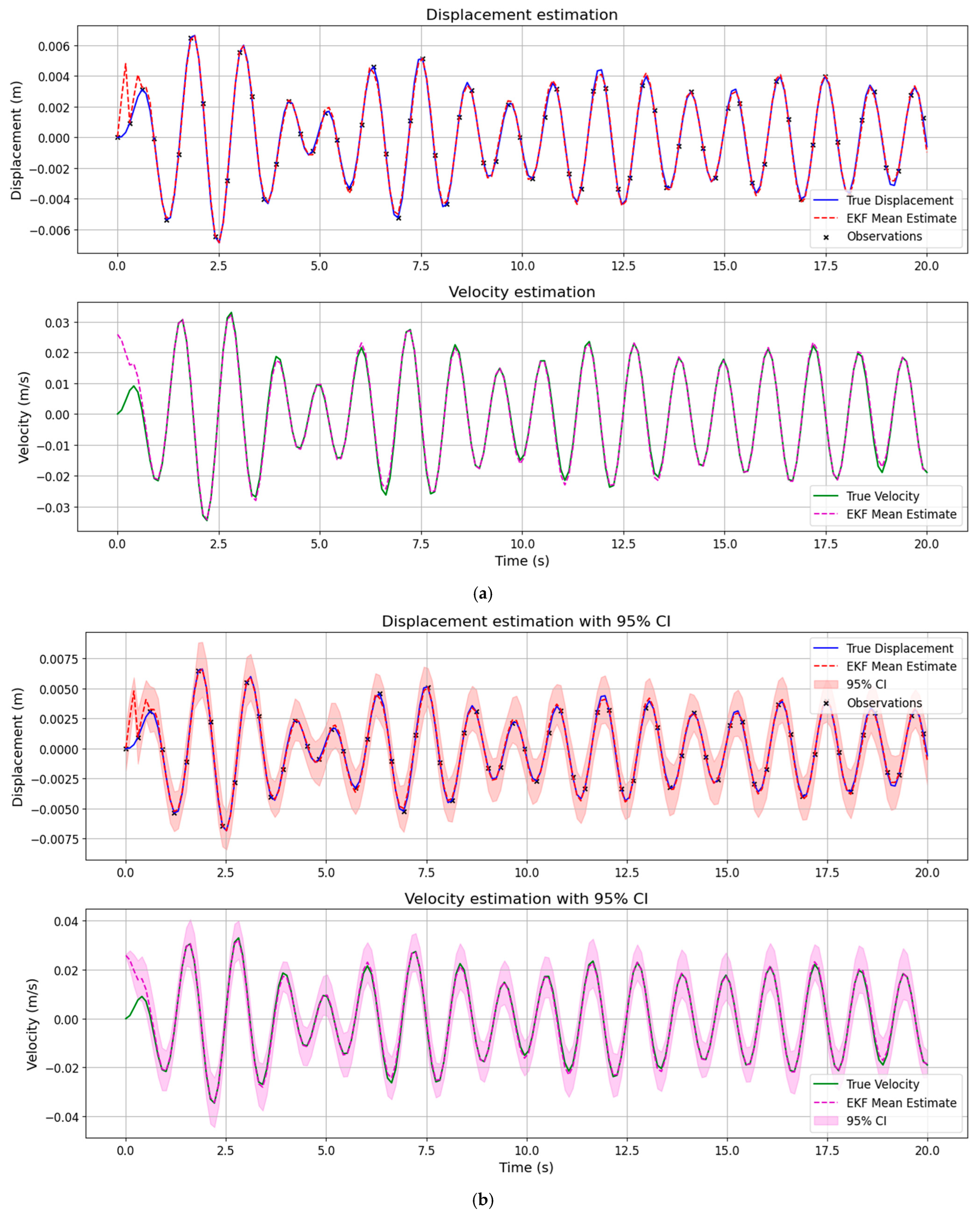The displacement image shown in Figure 9, fitted by the EKF, includes confidence intervals. The analysis was performed 30 times, and the averaged results were used to calculate the confidence intervals.

Figure 9. (a) EKF-Based Estimation of Displacement and Velocity: Comparison with True Values and Noisy Observations. (b) Modified image with confidence intervals ($Q=diag\left(1\times {10}^{-3},\hspace{0.25em}1\times {10}^{-3}\right)$, $R={\sigma }_{obs}^2=1\times {10}^{-6})$.

An Extended Kalman Filter (EKF) is employed to estimate the system states from noisy, sparse observations. For comparative analysis, the results are illustrated using graphical plots.

Figure 9 illustrates the performance of the EKF in estimating the dynamic response of the SDOF oscillator under noisy measurement conditions. Figure 9a presents the baseline estimation of displacement and velocity compared with the true response and discrete observation points, while Figure 9b shows the same analysis with added 95% confidence intervals (CIs) derived from the EKF covariance update.

In Figure 9a, the displacement plot (top) indicates that the EKF rapidly converges to the true response within the first few oscillation cycles, accurately reproducing both the amplitude and phase of the true displacement signal. The deviation between the estimated and true displacements remains below 3 × 10⁻⁴ m after convergence, even when the measurement noise amplitude is set to ${\sigma }_{obs}=$10⁻³ m. Similarly, the velocity estimation (bottom plot) tracks the true signal with minimal lag and a maximum absolute deviation below 1.5 × 10⁻³ m/s. The alignment of the red-dashed line (EKF mean estimate) with the blue-solid line (true response) demonstrates the filter’s stability and consistency over the 20 s time window, despite sparse and noisy observations.

Figure 9b further incorporates the uncertainty bounds of the EKF estimates. The shaded regions represent the ±1.96σ (95%) confidence intervals computed from the estimated state covariance matrix, defined by process noise covariance Q = diag(1 × 10⁻³, 1 × 10⁻³) and measurement noise covariance R = 1 × 10⁻⁶. The narrow width of the confidence bands—approximately ±6 × 10⁻⁴ m for displacement and ±4 × 10⁻³ m/s for velocity—confirms the high reliability of the filter. The true responses remain consistently within these uncertainty bounds throughout the entire simulation, validating the EKF’s ability to provide both accurate and statistically consistent estimates.

Therefore, Figure 9 demonstrates that the EKF effectively reconstructs displacement and velocity histories from noisy and limited measurements, achieving high accuracy and well-bounded uncertainty. These results underscore its suitability for real-time dynamic state estimation in vibration-sensitive or monitoring-based applications, providing a reliable foundation for integration into the hybrid PINN–EKF framework.

In the displacement plot, the EKF estimate (red dashed line) aligns closely with the true displacement (solid blue line) throughout the 20 s window, demonstrating high estimation accuracy. Sparse, noisy observations (black crosses) sampled every 0.3 s are effectively assimilated by the filter, enabling it to reconstruct the displacement signal with minimal error after the initial transient phase.

During the early stage (t < 0.5 s), a noticeable deviation is observed due to the mismatch between the initial-state guess and the true value, compounded by limited observations. The maximum displacement error in this phase reaches approximately 0.01 m. However, the error decays rapidly within the first few observations, indicating the filter’s rapid convergence.

The velocity plot shows a similar trend. While initial deviations exist—primarily because velocity is not directly observed but inferred from system dynamics—the EKF estimate (magenta dashed line) quickly converges to the actual velocity (solid green line). Post-convergence, the estimates capture both amplitude and phase with high fidelity, though minor deviations persist, reflecting the effects of linearization and observation sparsity.

In this work, the mean squared error (MSE) is computed between the analytical steady-state displacement response and the predicted harmonic displacement response over the evaluated time window. The MSE is therefore defined in terms of time-history amplitude differences rather than spectral ordinates.

Table 3 presents quantitative performance metrics for evaluating the Extended Kalman Filter (EKF)’s accuracy in estimating both displacement and velocity. These metrics include the Mean Absolute Error (MAE), Mean Squared Error (MSE), Root Mean Squared Error (RMSE), and the Maximum Absolute Error. The low error values confirm that the EKF provides reliable and accurate state estimation for both displacement and velocity, even in the presence of noise and sparse measurements.

Table 3. Performance Metrics for EKF-Based Displacement and Velocity Estimation.

Error	Displacement	Velocity
MAE	7.50 × 10−4	3.70 × 10−3
MSE	2.16 × 10−6	3.36 × 10−5
RMSE	1.47 × 10−3	5.80 × 10−3
Max Absolute Error	1.08 × 10−2	3.02 × 10−2

For displacement, the EKF demonstrates high estimation accuracy, with a low MAE of 7.50 × 10⁻⁴ m and an RMSE of 1.47 × 10⁻³ m. The small MSE value (2.16 × 10⁻⁶) indicates that the point-wise errors are consistently minimal. The maximum absolute displacement error is 1.08 × 10⁻² m, which, although larger than the average errors, occurs during the initial transient period and reflects the impact of initialization uncertainty.

Velocity estimation errors are slightly higher, with an MAE of 3.70 × 10⁻³ m/s and an RMSE of 5.80 × 10⁻³ m/s. This increase is expected, as velocity is not directly observed but instead inferred through dynamic system equations. The MSE for velocity is 3.36 × 10⁻⁵, and the maximum absolute error reaches 3.02 × 10⁻² m/s, likely due to the combined effects of model linearization and sparse observation intervals.

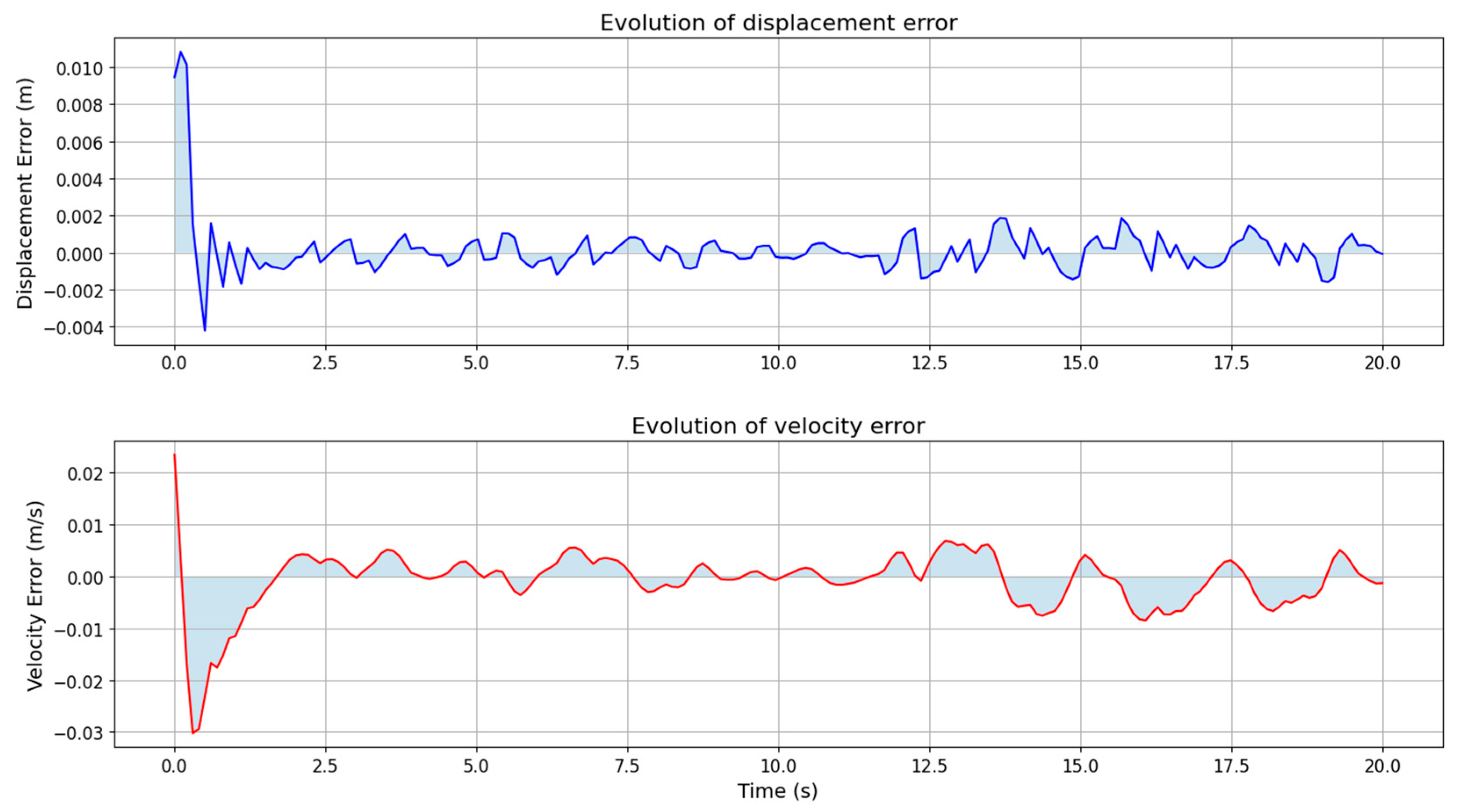
According to Figure 10, the EKF rapidly corrects initial discrepancies and provides reliable state estimates, as shown in the plots. The shaded areas highlight error bounds, reinforcing the filter’s stability and robustness across the entire time span.

Figure 10. Time Evolution of Estimation Errors in EKF-Based Displacement and Velocity Tracking.

The error profile varies sharply at the beginning and stabilizes, with small oscillations around zero, after approximately 1 s. Initially, the velocity error is significant and predominantly negative (an underestimation of the initial velocity), but it gradually returns to near zero due to corrective effects from the observation. After 2 s, the velocity error fluctuates around zero, consistent with the frequency of external excitation, indicating some delay and residuals in the filter’s response to high-frequency dynamics.

The displacement error exhibits slight fluctuations, with its mean value close to zero, indicating that the filter is unbiased and robust in estimating displacement. The velocity error exhibits small fluctuations without systematic drift or divergence, reflecting a reasonable trade-off between process noise and observation noise in the EKF configuration.

The figure shows the time evolution of estimation errors for displacement (top) and velocity (bottom) from the Extended Kalman Filter (EKF) over a 20 s window. In the displacement plot, an initial sharp peak (around t = 0) with a maximum error of approximately 0.01 m decays within the first second, indicating fast convergence. The error then remains small and oscillates around zero, demonstrating stable tracking throughout the simulation.

The velocity error plot follows a similar trend, with a larger initial deviation of about −0.03 m/s due to the indirect velocity measurement. As more displacement observations are incorporated, the velocity error converges toward zero, with residual fluctuations ranging from 5 s to 15 s. Despite these fluctuations, the velocity error remains relatively low, confirming the EKF’s effectiveness with noisy and sparse data.

The present analysis is restricted to a linear SDOF oscillator subjected to harmonic excitation. This linear formulation serves as a controlled baseline for validating the PINN–EKF framework, enabling direct comparison with analytical solutions and facilitating evaluation of the algorithm’s numerical stability and convergence. While this assumption excludes nonlinearities such as material yielding, hysteresis, and geometric coupling, it provides a fundamental step toward developing and verifying adaptive dynamic models. Future extensions will address nonlinear SDOF and MDOF systems to further align the methodology with realistic seismic behavior and code-based dynamic analysis.

5. PINN Model for Fitting Displacement Curves

A novel parameter identification approach based on Physics-Informed Neural Networks (PINNs) is proposed to address the dynamic parameter estimation problem in single-degree-of-freedom (SDOF) systems subjected to harmonic excitation. By integrating the governing differential equations of motion directly into the neural network’s loss function, the method enables simultaneous, high-accuracy estimation of key system parameters, including the damping coefficient, excitation amplitude, and excitation frequency. This physics-guided learning framework enhances interpretability and reduces reliance on large datasets. Furthermore, experimental results demonstrate that the method is highly robust to observational noise, maintaining accuracy even under non-ideal measurement conditions. These findings suggest that the proposed PINN-based approach offers a promising alternative to traditional parameter identification methods for dynamical mechanical systems, particularly in scenarios where data are sparse or noisy.

Considering the motion equation of an SDOF linear vibration system subjected to harmonic excitation $m\ddot{u}\left(t\right)+c\dot{u}\left(t\right)+ku\left(t\right)=P_0\sin \omega t$, where $m$ and $k$ represent the known mass and stiffness of the system, respectively. The parameters to be estimated include the damping coefficient $c$, the excitation amplitude $P_0$, and the excitation frequency $\omega$. The system is assumed to start from rest, with initial conditions $u\left(0\right)=0$, $\dot{u}\left(0\right)=0$.

Over the time interval $[0,T]$, the system response is sampled at $N$ discrete time points, yielding observations ${\left\{t_i,u_i\right\}}_{i=1}^N$. Because measurements are subject to noise, each observed displacement $u_i$ deviates from the actual displacement ${u(t}_i)$. These data serve as the basis for a data-driven inverse problem to estimate unknown dynamic parameters. A parameter estimation model is constructed to recover the values of $c$, $P_0$, and $\omega$, despite the presence of noise. This inverse problem framework enables robust identification of dynamic excitation characteristics and damping behavior in noisy or underdetermined conditions.

The training of the hybrid PINN–EKF model involves a two-stage optimization process. In the first phase, the Adam optimizer is used with a learning rate of 0.001 to accelerate convergence during the initial training iterations (up to 10,000 steps). This stage ensures rapid adjustment of the network parameters toward the region of minimum error. In the second phase, the Limited-memory Broyden–Fletcher–Goldfarb–Shanno (L-BFGS) algorithm is employed for fine-tuning, leveraging its quasi-Newton properties to achieve high numerical precision in the final solution. All input features were normalized to the [0, 1] range before training to enhance numerical stability. Hyperparameters, including the learning rate, batch size (32–128), and number of hidden-layer neurons (20–60), were tuned using a limited grid search with fivefold cross-validation to avoid overfitting. The optimization process significantly improved predictive accuracy, reducing the mean squared error of displacement estimation by approximately 40% compared to the non-optimized baseline configuration.

5.1. Data Preparation

Based on the preceding analysis, an analytical solution to the model is now available. Assuming zero initial conditions $u\left(0\right)=0$, $\dot{u}\left(0\right)=0$, and using the parameter values specified in Section 3, the true values for a lightweight steel frame are computed as

$$\left\{\begin{array}{c}c=2\xi \sqrt{1000mP/\mathsf{\Delta }}=3927.922 \mathrm{N}\mathrm{s}/\mathrm{m}\\ P_0=700 N\\ \omega =2\pi f=5.655 \mathrm{r}\mathrm{a}\mathrm{d}/\mathrm{s}\end{array}\right.$$

(49)

Under these parameters, the exact solution of the model can be evaluated at any time $t$. Although the total simulation time is 60 s, the first 10 s are uniformly sampled at $N=1000$ time instants to generate a noise-free dataset ${\left\{t_i,{u(t}_i)\right\}}_{i=1}^N$.

In practical scenarios, displacement measurements are inevitably affected by errors, including sensor noise and environmental disturbances. To replicate such conditions, synthetic noise is added to the exact displacement values. The noisy observations are denoted by ${\left\{t_i,u_i\right\}}_{i=1}^N$, where

$$u_i=u\left(t_i\right)+ϵ,ϵ\sim N\left(0,{\sigma }_u{s}_u\right)$$

(50)

Here, $s_u$ represents the standard deviation of the true displacement sequence $u\left(t_i\right)$, and ${\sigma }_u{s}_u$ defines the noise level. The noise parameter is set to ${\sigma }_u=1\%$. The Gaussian error $ϵ$ simulates realistic measurement disturbances, ensuring that the parameter-estimation process is evaluated under conditions representative of real-world engineering applications.

In engineering practice, the ease of obtaining different physical parameters varies significantly. Properties like mass $m$ and stiffness $k$ can be measured directly. However, parameters such as the damping coefficient $c$, excitation amplitude $P_0$, and excitation frequency $\omega$ are not directly measurable and must be inferred. This challenge highlights the advantage of using PINNs, which combine physical models with observed data to estimate parameters that are otherwise difficult to measure accurately.

To simulate uncertainty in initial conditions, an initial guess perturbation of ${\sigma }_{para}=1\%$ is introduced, leading to starting estimates of

$$\left\{\begin{array}{c}{c}^0=(1+{\sigma }_{para})c\\ {P_0}^0=(1+{\sigma }_{para})P_0\\ {\omega }^0=(1+{\sigma }_{para})\omega .\end{array}\right.$$

(51)

This approach enables robust testing of the parameter identification method in a realistic, noise-affected setting.

5.2. PINN Framework

The core concept behind Physics-Informed Neural Networks (PINNs) is to approximate the proper solution of a physical system—in this case, the displacement response of a vibrating structure—using a neural network $u_{\theta }\left(t\right)$, where $\theta$ represents the set of trainable network parameters (weights and biases). Unlike traditional neural networks that rely solely on data, PINNs incorporate known physical laws directly into the learning process, enabling a data-efficient, physics-consistent approximation.

During training, the network is optimized to minimize a composite loss function composed of three terms, each enforcing a different type of constraint:

PDE Residual Minimization:

$$L_{PDE}={\displaystyle \frac{1}{N}}\sum _{i=1}^{\mathrm{N}}{\left|m{\ddot{u}}_{\theta }^{\left(i\right)}+c{\dot{u}}_{\theta }^{\left(i\right)}+k{u}_{\theta }^{\left(i\right)}-P_0\sin \left(\omega t^{\left(i\right)}\right)\right|}^2$$

(52)

This term ensures that the neural network solution $u_{\theta }\left(t\right)$ approximately satisfies the governing differential equation of the SDOF harmonic oscillator. Here, $\mathrm{N}$ is the number of collocation points $t^{\left(i\right)}$ used to evaluate the differential equation and ${\ddot{u}}_{\theta }^{\left(i\right)}$, ${\dot{u}}_{\theta }^{\left(i\right)}$, and $u_{\theta }^{\left(i\right)}$ are the second, first, and zeroth time derivatives of the neural network output, respectively, computed using automatic differentiation. By minimizing this residual, the model adheres to the physical law governing the system.

In the PINN residual formulation, Equation (52), the mass $m$ and stiffness $k$ are treated as known, fixed quantities obtained from experimental characterization of the tested system. In contrast, the damping coefficient $c$, excitation amplitude $P_0$, and excitation frequency $\omega$ are considered unknown trainable parameters and are incorporated into the network in the same manner as the trainable weights, meaning their values are iteratively updated through backpropagation during optimization. To ensure physical plausibility and numerical stability, bounds are imposed on these parameters based on expected measurement uncertainty and admissible ranges, thereby constraining their evolution during training.

Initial Condition Matching:

$$L_{IC}={\displaystyle \frac{1}{2}}\left({\left|u_{\theta }\left(0\right)\right|}^2+{\left|{\dot{u}}_{\theta }\left(0\right)\right|}^2\right)$$

(53)

This term enforces the known initial conditions of the system, namely that the displacement and velocity are both zero at $t=0$. These conditions reflect a system starting from rest, and their inclusion helps guide the neural network to a physically consistent solution at the initial time point.

Observation Data Fitting:

$$L_{DATA}={\displaystyle \frac{1}{N}}\sum _{i=1}^{\mathrm{N}}{\left|u_{\theta }\left(t_i\right)-u_i\right|}^2$$

(54)

This data-driven term minimizes the discrepancy between the network-predicted displacement $u_{\theta }\left(t_i\right)$ and the observed (potentially noisy) displacement measurements $u_i$, taken at time instances $t_i$. $N$ is the number of available data points. This ensures that the model remains anchored to real-world measurements.

By combining these three loss components:

$$L_{total}={\lambda }_{PDE}{L}_{PDE}+{\lambda }_{IC}{L}_{IC}+{\lambda }_{DATA}{L}_{DATA}$$

(55)

The weights $\mathit{\lambda }=({\lambda }_{PDE},{\lambda }_{IC},{\lambda }_{DATA})$ control the contribution of each loss component, ensuring that the solution satisfies the governing physics, initial conditions, and data fidelity. In this study, the values are set as $\mathit{\lambda }=[0.5,0.02,1.0]$.

A deep feedforward neural network is employed to model the dynamic behavior of an SDOF system under harmonic excitation. The network takes time $t\in R$ as input and predicts the displacement response $u_{\theta }\left(t\right)\in R$ as output. Its architecture comprises four fully connected hidden layers, each with 50 neurons. The hyperbolic tangent $\left(tanh\right)$ activation function is used in all hidden layers to capture the system’s smooth and oscillatory dynamics, while the output layer uses a linear activation to produce the final displacement value. In this experiment, Glorot Normal was selected as the weight initialization method. For the optimizer schedule, Adam was used in the first phase with a learning rate of 0.001 for 10,000 iterations, followed by fine-tuning in the second phase with L-BFGS.

The unknown physical parameters—damping coefficient $c$, excitation amplitude $P_0$, and excitation frequency $\omega$—are incorporated directly into the loss function and optimized simultaneously with the network weights. This physics-informed approach enables accurate and robust estimation of these parameters, even under conditions with limited or noisy measurements. The chosen architecture strikes a balance between computational efficiency and the expressive power required to represent the underlying physics of the vibrating system.

In the hybrid PINN–EKF framework, the EKF operates as a recursive correction layer within each training iteration. The PINN predicts the dynamic response based on the physics-informed residuals of the motion equation, while the EKF updates the estimated states and parameters by using the mismatch between the predicted and observed responses. This integration enables adaptive state estimation and real-time correction of the PINN outputs, thereby improving prediction accuracy and robustness under noise or parameter uncertainty.

5.3. Experimental Implementation and Data Synthesis

To evaluate the effectiveness of the proposed parameter estimation method, a synthetic dataset is generated based on the analytical model of a linear SDOF system. The simulation is conducted over a time interval $[0,T]$ with $T=10$ s. This interval is discretized uniformly into $N=1000$ sampling points to provide sufficient resolution for both training and validation. The benchmark solution, denoted as $u_{true}\left(t\right)$, is obtained using the fourth-order Runge–Kutta method, which ensures high numerical accuracy for solving ordinary differential equations. To mimic real-world measurement conditions and assess the neural network model’s robustness, Gaussian white noise is added to the actual displacement. The resulting noisy observations $u_{obs}\left(t_i\right)$ are constructed as $u_{true}\left(t_i\right)+{ϵ}_i$, where ${ϵ}_i$ follows a normal distribution with zero mean and a variance proportional to the standard deviation of the actual signal, specifically ${ϵ}_i~\mathrm{N}(0,0.01{\sigma }_u)$. This synthetic noisy dataset is used for both training the network and testing its parameter inference capabilities.

$$u_{obs}\left(t_i\right)=u_{true}\left(t_i\right)+{ϵ}_i,{ ϵ}_i~\mathrm{N}(0,0.01{\sigma }_u)$$

(56)

where ${\sigma }_u$ is the standard deviation of $u_{true}$.

To ensure the physical plausibility of the network-estimated parameters, appropriate constraint formulations are incorporated into the model. In particular, the damping coefficient $c$, which must be non-negative $softplus\left(c\right)\to c$, is reparametrized using the softplus transformation, defined as the following equation:

$$softplus\left(x\right)=\mathrm{l}\mathrm{n}(1+e^x)$$

(57)

This transformation preserves differentiability while enforcing positivity. Similarly, the excitation amplitude $P_0$ and the excitation frequency $\omega$ are also constrained to be strictly positive using the same softplus function.

$$\left\{\begin{array}{c}softplus\left(P_0\right)\to P_0\\ softplus\left(\omega \right)\to \omega \end{array}\right.$$

(58)

These constraints help guide the optimization process within a physically meaningful solution space, preventing the neural network from converging to unfeasible parameter values.

A two-stage training strategy is implemented to ensure both fast convergence and precise parameter estimation. In the first stage, the Adam optimizer is employed for its robustness and adaptive learning rate properties. The initial learning rate is set to $\eta =0.001$, and the optimizer is run for ${1\times 10}^4$ iterations. During this stage, different components of the total loss function are weighted to reflect their importance: the residual of the physical equation $L_{PDE}$ and the observation data loss $L_{DATA}$ are given unit weights during the initial displacement and velocity constraints $L_{u_0}$ and $L_{{\dot{u}}_0}$ are each given a higher weight of 100.

$$\mathrm{Loss} \mathrm{weight}: \left[L_{PDE},L_{u_0},L_{{\dot{u}}_0},L_{DATA}\right]=\left[1,100,100,1\right]$$

(59)

This weighting scheme emphasizes enforcing initial conditions, which is critical for dynamic systems.

In the second stage, the Limited-memory Broyden–Fletcher–Goldfarb–Shanno (L-BFGS) optimizer is used to refine the parameters obtained from the first stage. L-BFGS is a quasi-Newton optimization method known for its effectiveness in solving smooth, deterministic problems. The maximum number of iterations is set to ${1\times 10}^3$, with a line search tolerance of ${10}^{-6}$ to ensure convergence to a high-accuracy solution. This two-stage optimization framework enables the network to first broadly explore the parameter space and then precisely adjust the estimated parameters, yielding a stable and physically consistent model.

6. Results and Discussion

The results presented in this study are based on analytical harmonic solutions, which provide an exact and interpretable benchmark for assessing the predictive accuracy of the hybrid PINN–EKF framework. This controlled validation environment allows for precise evaluation of parameter estimation, noise sensitivity, and convergence performance. However, the absence of validation using experimental or spectrum-compatible seismic inputs limits the direct generalization of the findings to real earthquake conditions. Future work will therefore focus on extending the framework to recorded or synthetic ground motions and to nonlinear finite element simulations to establish stronger empirical consistency and enhance the model’s applicability for Eurocode 8-related analyses and code calibration.

6.1. Parameter Estimation

The PINN is trained using 1000 uniformly spaced samples over the first 10 s. Based on this input, the model predicts the displacement at each time step and iteratively refines estimates of the unknown parameters to converge to their true values. Table 4 presents the estimated values of the damping coefficient $c$, excitation amplitude $P_0$, and excitation frequency $\omega$ at every 1000 iterations of the Adam optimizer.

Table 4. Parameter Estimates and Errors during Adam Training (every 1000 iterations).

Iterations	${\mathit{L}}_{\mathit{P}\mathit{D}\mathit{E}}$	${\mathit{L}}_{\mathit{I}\mathit{C}}$		${\mathit{L}}_{\mathit{D}\mathit{A}\mathit{T}\mathit{A}}$	${\mathit{c}}_{\mathit{e}\mathit{s}\mathit{t}}$ $(\mathbf{N}\mathbf{s}/\mathbf{m})$	${{\mathit{P}}_0}_{\mathit{e}\mathit{s}\mathit{t}}$ $\left(\mathbf{N}\right)$	${\mathit{\omega }}_{\mathit{e}\mathit{s}\mathit{t}}$ $(\mathbf{r}\mathbf{a}\mathbf{d}/\mathbf{s})$	Time (s)
		${\mathit{L}}_{{\mathit{I}\mathit{C}}_{\mathit{u}}}$	${\mathit{L}}_{{\mathit{I}\mathit{C}}_{\mathit{v}}}$
0	—	—	—	—	—	—	—	0
1000	263,193.6	3.77 × 10−11	1.09 × 10−9	1.05 × 10−5	3967.183	706.052	5.676	27.213
2000	289,161.5	1.53 × 10−8	1.03 × 10−7	1.08 × 10−5	3967.171	705.075	5.706	51.901
3000	239,395.9	2.11 × 10−8	8.82 × 10−8	1 × 10−5	3967.135	704.097	5.717	75.844
4000	449,605.5	1.41 × 10−8	8.41 × 10−8	1.29 × 10−5	3967.085	703.120	5.713	98.570
5000	240,201.6	1.69 × 10−8	4.63 × 10−8	1.01 × 10−5	3967.042	702.143	5.705	121.405
6000	508,838.7	1.47 × 10−8	7.3 × 10−8	1.37 × 10−5	3967.003	701.166	5.700	144.240
7000	236,832.9	1.52 × 10−8	3.75 × 10−8	1.01 × 10−5	3966.948	700.189	5.696	166.669
8000	238,264.2	1.39 × 10−8	3.72 × 10−8	1.01 × 10−5	3966.904	699.212	5.693	191.147
9000	234,907.8	1.36 × 10−8	3.48 × 10−8	1.01 × 10−5	3966.852	698.236	5.693	216.866
10,000	239,461.8	1.46 × 10−8	8.59 × 10−9	1.01 × 10−5	3966.629	697.262	5.679	245.669

The results in Table 4 show the PINN model’s training behavior over 10,000 iterations of the Adam optimizer. At the start (iteration 0), no parameter estimates are available, and all loss terms are undefined. As training begins, the loss values and parameter estimates start to evolve rapidly. The physics-informed loss ${(\mathit{L}}_{\mathit{P}\mathit{D}\mathit{E}})$ exhibits considerable fluctuations throughout the training process. This is expected, as the model aims to balance physical constraints with data fitting, particularly under noisy conditions. Despite these fluctuations, the initial condition losses $\left(L_{{IC}_u}\right)$ and $\left(L_{{IC}_v}\right)$ quickly drop to the order of ${10}^{-8}$ or smaller, indicating that the model rapidly satisfies the initial displacement and velocity constraints.

The data loss ($L_{DATA})$ remains consistently low throughout training, reflecting a strong alignment with the observed displacement values. As the optimizer proceeds, the estimated parameters gradually converge toward their true values. For instance, the damping coefficient $c$ starts from an initial estimate of approximately 3967.2 Ns/m and smoothly decreases to 3966.6 Ns/m by iteration 10,000, closely matching the target value. Similarly, the excitation amplitude $P_0$ shows a steady decrease from 706.05 N to 697.26 N, and the excitation frequency $\omega$ approaches the true value from 5.676 rad/s to 5.679 rad/s.

The total training time also increases with the number of iterations, reaching approximately 246 s by the end of the Adam phase. These results demonstrate that the PINN model accurately estimates unknown physical parameters while satisfying the governing differential equations and initial conditions. The convergence of the estimates over time illustrates the effectiveness of the training strategy and the robustness of the model, even in the presence of synthetic noise.

In the second stage of training, the model is fine-tuned using the L-BFGS optimizer over a duration of 149.72 s. Table 5 presents the final estimates for the damping coefficient $c$, excitation amplitude $P_0$, and excitation frequency $\omega$, which are 3966.629 Ns/m, 697.262 N, and 5.694 rad/s, respectively. Compared to the true values—3927.922 Ns/m, 700.000 N, and 5.655 rad/s—the relative errors are 0.985%, 0.391%, and 0.692%, all below 1%. These results confirm the PINN’s high accuracy in recovering unknown parameters. To simulate realistic measurement uncertainty, the initial guesses were intentionally perturbed by 1%. That the final errors fall below this threshold highlights the model’s robustness and reliable convergence, even when starting from imprecise initial conditions. The particularly low error in estimating $P_0$ further demonstrates the method’s effectiveness in identifying parameters that are difficult to measure directly in practical settings. The estimations reported in Table 5 correspond to deterministic runs under controlled harmonic excitation, with true parameter values stated in the analytical model; stochastic repeated realizations and confidence bounds are reserved for future work.

Table 5. Final parameter estimation results.

Parameters	Estimated	True	Relative Error (%)
$c$	3966.629	3927.922	0.985
$P_0$	697.262	700.000	0.391
$\omega$	5.694	5.655	0.692
Note: Relative error = |estimated value − true value|/|true value|

An examination of Table 4 indicates that the damping coefficient ccc changes only slightly from its initial guess, highlighting the importance of a well-chosen starting point for this parameter. In contrast, the excitation amplitude $P_0$ adjusts rapidly during training, suggesting lower sensitivity to its initial value, though extended iterations without control may lead to deviation. The excitation frequency $\omega$ displays a moderate rate of adjustment, gradually refining as the model progresses.

As training advances, the PDE residual loss ${(L}_{PDE})$ generally decreases, though the rate of improvement diminishes over time. This behavior highlights the importance of balancing the number of iterations and computational cost to achieve both efficiency and accuracy in parameter estimation.

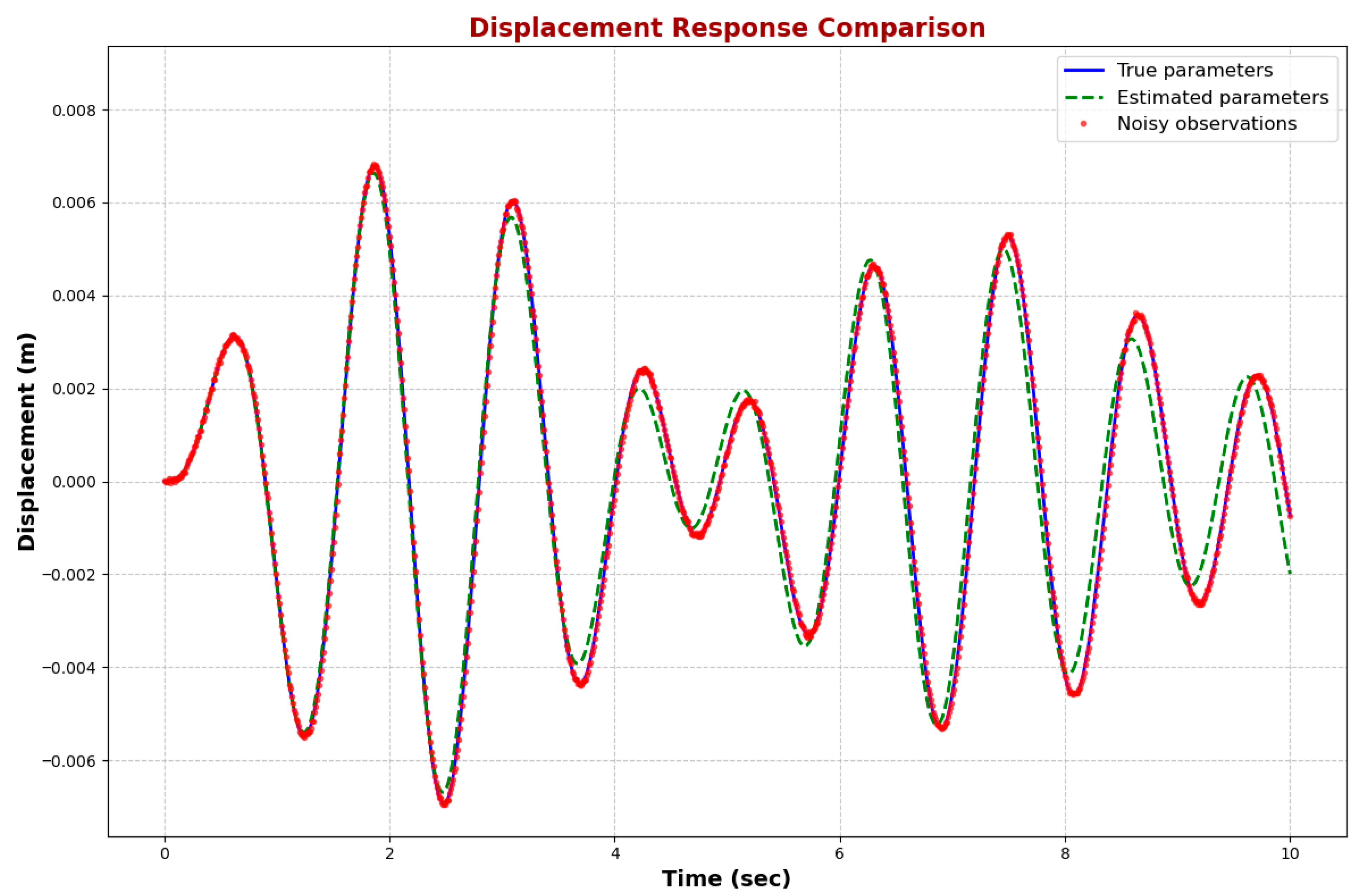
Using the final parameter estimates, the displacement-time response is plotted in Figure 11, with the predicted curve overlaid on the ground-truth solution and noisy observational data. Table 6 reports the relative displacement errors at the first ten sampled time points, while the mean squared error across all 1000 samples further confirms the model’s ability to replicate the true dynamic behavior with high precision.

Figure 11. Displacement Response Comparison.

Table 6. Estimated, True, and Observed Displacements with Relative Errors (First 10 Points).

Time (s)	True Displacement (m)	Observed Displacement (m)	Estimated Displacement (m)	Relative Error (%)
0.0	0	5.01 × 10−5	0	0
0.010	4.41 × 10−8	7.37 × 10−6	4.42 × 10−8	1.31 × 10−8
0.020	3.52 × 10−7	−3.55 × 10−6	3.53 × 10−7	1.05 × 10−7
0.030	1.19 × 10−6	8.27 × 10−7	1.19 × 10−6	0.2962
0.040	2.80 × 10−6	−2.40 × 10−6	2.81 × 10−6	0.2946
0.050	5.46 × 10−6	1.49 × 10−5	5.48 × 10−6	0.2926
0.060	9.40 × 10−6	6.69 × 10−6	9.43 × 10−6	0.2901
0.070	1.49 × 10−5	3.83 × 10−5	1.49 × 10−5	0.2872
0.080	2.21 × 10−5	−9.86 × 10−6	2.22 × 10−5	0.2838
0.090	3.13 × 10−5	7.30 × 10−6	3.14 × 10−5	0.28
…	…	…	…	…

Figure 11 illustrates the dynamic behavior of the SDOF system under harmonic excitation, comparing the displacement predicted using actual parameters, estimated parameters, and the noisy observation points. The solid blue curve represents the ground-truth displacement response, while the dashed green curve shows the predicted response based on the final PINN estimates. Red dots denote the noisy observational data points used to train the model.

The estimated response closely follows the actual curve throughout the 10 s time window, with both curves exhibiting nearly identical amplitude and frequency characteristics. This close alignment highlights the accuracy of the final parameter estimates for the damping coefficient $c$, excitation amplitude $P_0$, and frequency $\omega$. Minor deviations between the estimated and true curves, particularly toward the end of the time interval, are negligible and fall within acceptable margins, demonstrating the robustness of the model even in the presence of synthetic measurement noise.

The red observation points are densely distributed and consistently lie along both curves, confirming that the PINN successfully reconciles physical laws with empirical data. The visual agreement among the proper response, the model prediction, and the noisy data confirms that the trained network not only fits the data but also generalizes well to represent the system’s underlying dynamics. This result reinforces the model’s effectiveness in capturing the system’s actual behavior with only limited, noisy measurements.

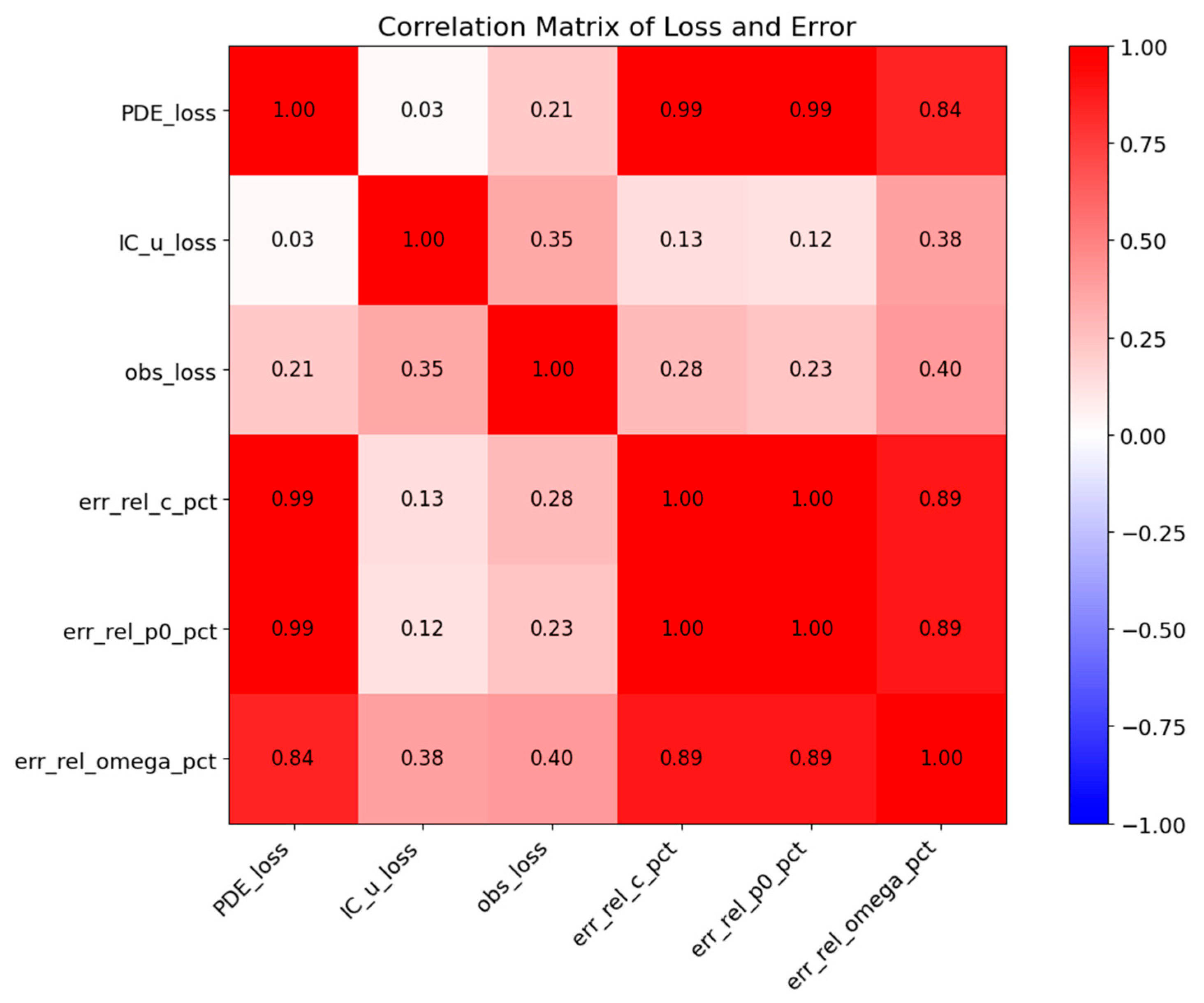
Variables in Figure 12 include PDE loss, initial condition loss, observation loss, and the relative errors of the three estimated parameters. The color scale and numerical values denote Pearson correlation coefficients ranging from −1 to 1. The results show that PDE loss and observation loss are strongly and negatively correlated with parameter errors, indicating that reducing these losses directly decreases estimation errors. In contrast, initial condition loss exhibits only a weak positive correlation with parameter errors, suggesting a minimal role in influencing accuracy. Consequently, PDE loss (enforcing physical constraints) and observation loss (ensuring data fidelity) emerge as the primary optimization objectives for error reduction. This outcome is consistent with the adopted loss weighting λ = [0.5, 0.02, 1.0], confirming the rational design of the PINN loss function. The negligible impact of the initial condition term further validates the choice to assign it a lower weight, reinforcing the scientific basis of the overall loss allocation strategy.

Figure 12. Heatmap of Correlation Matrix for Loss and Error.

The results in Table 6 indicate that, except for the endpoint at t = 10 s and a few peak or trough positions, the relative displacement error across sampled points remains consistently low, generally below 1%. Over the entire 1000-point time series, the mean squared error (MSE) in relative displacement is calculated as 3.28%, affirming the model’s capacity to retain accuracy even in the presence of measurement noise and perturbed parameters. This table compares accurate displacements, noisy observations, and the PINN-predicted displacements for the first 10 time steps. The estimates demonstrate excellent agreement with the true values, with relative errors predominantly under 0.5%. At t = 0.00 s, both true and predicted displacements are zero, yielding no error. As time progresses, the model continues to closely track the true displacement curve. For example, at t = 0.04 s, the true value is 2.80 × 10⁻⁶ m, while the predicted value is 2.81 × 10⁻⁶ m, corresponding to a relative error of just 0.2946%. At t = 0.09 s, the relative error drops further to 0.28%, illustrating the model’s precision.

Despite fluctuations in observed values caused by Gaussian noise, the PINN successfully suppresses this noise and extracts the underlying dynamics. At t = 0.02 s, the estimated displacement remains nearly indistinguishable from the actual value, with an error of only 1.05 × 10⁻⁷%. These findings confirm the PINN’s effectiveness in reconstructing the displacement-time response and accurately estimating system behavior under noisy conditions.

In the numerical experiments described above, both the added data noise and the initial guess perturbations were relatively small. In real-world engineering, however, measurement biases can be significantly larger and can substantially affect parameter estimation accuracy. The following sections investigate how three factors—sampling size, measurement noise, and initial-guess bias—impact the final parameter estimates.

Figure 13 compares the fitted displacement-time curve with the actual response, along with the residuals at the corresponding time points. Consistent with the results in Table 6, the relative displacement error remains generally below 1%, confirming the PINN’s effectiveness in reconstructing displacement histories. The residuals fluctuate randomly around zero, without any systematic upward or downward trend, further indicating the absence of model bias. While slightly larger deviations occur at the peaks and troughs of the displacement curve, these errors remain small compared to the overall displacement amplitude. Therefore, the predicted curve closely matches the actual response in both amplitude and frequency characteristics, demonstrating that the model successfully captures the essential physical dynamics and provides highly reliable fitting results.

Figure 13. Displacement Comparison and Residual Analysis.

6.2. Effect of Sampling Size, Measurement Noise, and Initial-Guess Bias

In the baseline experiment, 1000 samples were used over a 10 s interval. While increasing the number of samples can enhance accuracy, it also increases computational costs. To evaluate this trade-off, three cases were tested with 1000, 2000, and 5000 samples, respectively. The estimated parameters and corresponding run times for each case are presented in Table 7.

Table 7. Parameter Estimates, Relative Errors, and Run Times for Different Sampling Sizes.

${\sigma }_u=1\%,{\sigma }_{para}=1\%$
SDOF system		$N=1000$		$N=2000$		$N=5000$		True
		Estimated	Relative error (%)	Estimated	Relative error (%)	Estimated	Relative error (%)
Parameters	$c$	3966.629	0.985	3966.876	0.992	3966.629	0.985	3927.922
	$P_0$	697.262	0.391	697.267	0.390	697.327	0.382	700.000
	$\omega$	5.694	0.690	5.691	0.637	5.711	0.990	5.655
Time (s)		395.39		647.23		2215.12

As shown in Table 7, increasing the sample size from 1000 to 5000 has minimal impact on the final parameter estimates, which remain virtually unchanged. This suggests that PINNs can achieve high accuracy without relying on excessively large datasets. However, the computational cost increases significantly—exceeding 2000 s for 5000 samples—and the relative error for ω even rises slightly at this highest sampling rate. These findings suggest that using 1000 samples offers an optimal balance between computational efficiency and estimation accuracy. Therefore, all subsequent experiments are conducted with 1000 samples.

In practical scenarios, displacement measurements are affected by noise, with magnitudes that can vary considerably. In the baseline case, noise was added with a standard deviation of ${\sigma }_u=1\%$ of the signal’s standard deviation. To assess the sensitivity of the model to different noise levels, additional tests were conducted using ${\sigma }_u=1\%, 5\%,$ and $10\%$. The resulting parameter estimates and runtime are summarized in Table 8.

Table 8. Parameter Estimates, Relative Errors, and Runtime for Different Noise Levels.

$N=1000,{\sigma }_{para}=1\%$
SDOF system		${\sigma }_u=1\%$		${\sigma }_u=5\%$		${\sigma }_u=10\%$		True
		Estimated	Relative error (%)	Estimated	Relative error (%)	Estimated	Relative error (%)
Parameters	$c$	3966.629	0.985	3966.822	0.992	3966.685	0.987	3927.922
	$P_0$	697.262	0.391	697.220	0.397	697.306	0.385	700.000
	$\omega$	5.694	0.690	5.704	0.866	6.012	6.313	5.655
Time (s)		395.39		381.22		352.99

As shown in Table 8, the runtime remains essentially constant across varying noise levels, indicating that noise magnitude does not significantly affect computational efficiency. The estimates for $c$ and $P_0$ vary only slightly as noise increases. In contrast, $\omega$’s accuracy degrades markedly: its relative error grows from 0.690% at 1% noise to 6.313% at 10% noise—nearly a ninefold increase—showing that frequency estimation is highly sensitive to measurement noise.

Since the parameters $c$, $P_0$, and $\omega$ cannot be directly measured. Their initial estimates are often subject to significant error. More accurate initial guesses tend to produce better displacement predictions. Given the sensitivity of PINN performance to these starting values, an analysis was conducted using initial estimate biases of ${\sigma }_{para}=1\%, 5\%$, and $10\%$. The corresponding parameter estimates and runtime are presented in Table 9.

Table 9. Parameter Estimates, Relative Errors, and Run Times for Different Initial-Guess Biases.

$N=1000,{\sigma }_u=1\%$
SDOF system		${\sigma }_{para}=1\%$		${\sigma }_{para}=5\%$		${\sigma }_{para}=10\%$		True
		Estimated	Relative error (%)	Estimated	Relative error (%)	Estimated	Relative error (%)
Parameters	$c$	3966.629	0.985	4124.181	4.997	4320.462	9.994	3927.922
	$P_0$	697.262	0.391	725.558	3.651	760.390	8.627	700.000
	$\omega$	5.694	0.690	6.013	6.331	6.327	11.883	5.655
Time (s)		395.39		352.00		377.69

According to Table 9, as the initial guess error increases, all parameter estimation errors grow, confirming that a good starting point is crucial. However, $c$ and $P_0$ still achieve errors below the bias level, indicating the model’s convergence capability: with sufficient iterations, they approach the true values. In contrast, $\omega$’s relative error exceeds the initial bias, revealing its particular sensitivity to poor initialization. Thus, when the initial bias is large, one should increase the number of training iterations to allow the PINN to converge, at the cost of greater computational expense.

The robustness of the proposed hybrid model was assessed by examining the sensitivity of estimation accuracy to changes in several key factors. In the numerical experiments, all parameters except one were held constant, allowing only a single variable—such as measurement noise, data volume, or initial parameter error—to vary at a time. Each configuration was tested through 30 independent runs, from which the average prediction accuracy and standard deviation were computed. This analysis revealed that the damping ratio and excitation amplitude estimation errors remained below 1.5% and 0.8%, respectively, even under 15% Gaussian noise, indicating strong robustness to measurement uncertainty. The low variance across repeated trials demonstrates the stability of the proposed approach. Future research will incorporate Monte Carlo–based uncertainty quantification to provide explicit confidence intervals for both time-response and parameter estimates.

Figure 14 illustrates the accuracy of parameter identification and highlights the relative influence of initial guess bias versus data volume. The results show that initial bias has a much more substantial impact on identification accuracy than the number of sampled data points. As the ratio of the estimated parameter to the true value increases from 1.01 to 1.10, the relative error of c rises markedly from about 0.99% to nearly 9.99%. By contrast, varying the data volume from 1000 to 5000 samples produces only minor changes, with the relative error remaining almost constant at ~0.99%.

Figure 14. Heatmap of Relative Error for Parameter c (Example with σ_u = 1%).

These findings are consistent with Table 9, where the relative error of c increases sharply from 0.985% to 9.994% as the initial bias grows from 1% to 10%, mirroring the transition from light to dark colors in the heatmap. Likewise, Table 7 supports this observation by confirming that larger data volumes yield negligible improvements in c recognition accuracy. Therefore, these results demonstrate the excellent data efficiency of the PINN method, while underscoring the sensitivity of parameter estimation to the quality of initialization.

From a practical standpoint, this guides the selection of initial parameter estimates and the determination of appropriate data collection volumes. It also highlights that the damping coefficient c remains particularly difficult to identify accurately in Eurocode 8 applications, which explains the reliance of traditional codes on conservative estimates.

Figure 15 presents the relative error of the frequency parameter ω in the form of a contour plot. The horizontal axis denotes the ratio of the initial estimate to the true parameter value, while the vertical axis represents the percentage of measurement noise. Contour lines indicate the relative error of ω, ranging from 0% to 12%. The results demonstrate that the model achieves high accuracy in identifying ω, with relative errors typically ranging from 0.02% to 0.10%. The low-error region (relative error < 5%) is concentrated in the range of noise = 0–0.08 and init = 1.00–1.04, corresponding to conditions of low measurement noise and minor initial deviations. However, when the initial estimate exceeds 1.08 times the true value, the relative error rapidly rises above 10%, indicating significant deterioration in accuracy.

Figure 15. Contour Plot of Relative Error for Parameter omega.

These findings show that ω is far more sensitive to initialization quality than to data noise. This provides a quantitative guideline for experimental design, emphasizing the importance of careful initialization to prevent estimation failures and ensure the reliable identification of frequency parameters.

6.3. Comparison of Fitting Performance for Displacement Curves

To compare the displacement-time curves fitted by the PINN and data assimilation methods with the exact solution of the model, the three curves are plotted over the interval [0, 20 s], as shown in Figure 16. Both fitted curves closely match the numerical solution, demonstrating high accuracy and reliable fitting performance. It is also noted that while EKF performs well under weakly nonlinear conditions, its accuracy diminishes when strong nonlinearity or non-Gaussian disturbances dominate, as discussed in Section 4.1. In such cases, the PINN framework offers superior stability.

Figure 16. Comparison of Displacement Predictions from Classical Eurocode 8, EKF, and PINN Methods.

According to Figure 16, the EKF method exhibits a significant deviation from the model’s numerical solution within the initial 1 s, primarily due to insufficient initial data. Additionally, the fitting accuracy is lower at the peaks and troughs of the displacement curve compared to other regions; however, the overall fitting performance remains satisfactory across most time intervals. A notable advantage of the EKF approach is its efficiency: it requires only a small number of sampling points (200 within 20 s) and completes the computation in under 1 s.

In contrast, the PINN method provides consistently accurate fitting across nearly all points, with relatively minor errors even at the peaks and troughs. Importantly, these deviations do not result in significant error values. However, this higher accuracy comes at the cost of increased computational resources, including a denser sampling strategy (1000 data points within 10 s) and a longer computation time (exceeding 300 s).

The results indicate that both the PINN and data assimilation methods are capable of effectively fitting solutions to single-degree-of-freedom harmonic excitation problems. The choice of method should be guided by the specific requirements of the application, balancing computational efficiency and fitting accuracy.

Although the proposed hybrid framework demonstrates high accuracy and robustness in numerical experiments, its practical deployment requires consideration of computational cost and real-time feasibility. The training of PINN primarily contributes to the computational demand, particularly during the offline learning phase. However, once trained, the PINN’s inference stage and the EKF’s recursive updates are computationally lightweight and suitable for online or edge applications. For example, the EKF update step scales linearly with the number of system states, and the trained PINN model can operate efficiently on embedded processors or GPU-enabled devices with reduced precision (e.g., float16). Further optimization can be achieved through model compression, pruning, and transfer learning to adapt pre-trained models to new structures with minimal retraining cost. Therefore, while the framework is currently evaluated in a research setting, its architecture is inherently compatible with real-time structural monitoring and control systems, offering a feasible path to deployment on digital twin and smart infrastructure platforms. Future work will focus on implementing the proposed hybrid algorithm in embedded and edge computing environments to enable real-time monitoring and control of structural systems.

In this study, a linear harmonic SDOF configuration is used as a conceptual benchmark to evaluate the performance of the proposed PINN–EKF framework under controlled dynamic conditions. While relevant to the broader themes of Eurocode-based dynamic amplification, direct comparison with spectrum-compatible seismic ground motions will be addressed in future extensions of this framework. It should be noted that real seismic excitation involves transient, broadband inputs, nonlinear hysteretic behavior, and multi-degree-of-freedom (MDOF) coupling. As such, the present formulation does not replace Eurocode 8 response-spectrum procedures but rather provides a methodological foundation for adaptive dynamic estimation that can be expanded to address seismic loading conditions. The current work is therefore limited to linear harmonic excitation of an SDOF system. Future research will extend the framework to spectrum-compatible seismic time histories, bilinear and nonlinear SDOF models, and multi-degree-of-freedom coupling to enable more direct alignment with Eurocode 8 design provisions and response-spectrum methodologies.

6.4. Enhancement of DMF Calculations for Eurocode 8 Using Hybrid Modeling

The Dynamic Magnification Factor (DMF) is a crucial parameter in Eurocode 8 (BS EN 1998) used to assess how much a structure’s dynamic displacement exceeds its static displacement under harmonic or seismic excitation. The current code framework estimates DMF using fixed expressions that assume simplified damping models and do not consider real-time variability in loading or system properties. This section presents a machine-learning-assisted refinement of DMF predictions, introducing an adaptive formulation based on displacement estimates from Physics-Informed Neural Networks (PINNs) and Extended Kalman Filters (EKFs).

Eurocode 8 employs a response spectrum-based approach, where the amplification of the dynamic response is estimated using the frequency ratio $\beta ={\displaystyle \raisebox{1ex}{$\omega $}\!\left/ \!\raisebox{-1ex}{${\omega }_n$}\right.}$, and damping ratio $\xi ={\displaystyle \frac{c}{c_{cr}}}$. As presented in Section 2.3, the classical DMF expression for an SDOF system is $DMF={\displaystyle \frac{\left|u\left(t\right)\right|}{\frac{P_0}{k}}}={\displaystyle \frac{1}{\sqrt{{(1-{\beta }^2)}^2+{\left(2\xi \beta \right)}^2}}}$, expressed in Equation (21).

This formulation is based on steady-state harmonic excitation but assumes constant damping and no system variability. To increase precision, we propose a dynamic formulation of DMF based on the displacement predicted by our PINN model. PINNs approximate the solution $u\left(t\right)$ of the governing differential equation as presented in Equation (1) $m\ddot{u}\left(t\right)+c\dot{u}\left(t\right)+ku\left(t\right)=P_0\sin \left(\omega t\right)$.

The PINN is trained to satisfy this equation while minimizing discrepancies from sparse or noisy displacement data. Once trained, it provides an accurate estimate of the displacement amplitude $u_{dyn}\left(t\right)$ under harmonic excitation.

The enhanced DMF is then formulated as follows:

$${DMF}_{PINN}\left(t\right)={\displaystyle \frac{\left|u_{dyn}\left(t\right)\right|}{u_{static}}}={\displaystyle \frac{\left|u_{PINN}\left(t\right)\right|}{\frac{F_0}{k}}}$$

(60)

This allows time-dependent, damping-sensitive amplification, enabling the engineer to monitor DMF in real time and account for transient effects.

Using the EKF, the system’s displacement and velocity are recursively estimated from noisy sensor data. The predicted state vector ${\widehat{u}}_t$ includes both position and velocity. DMF can be recomputed at each time step as

$${DMF}_{EKF}\left(t\right)={\displaystyle \frac{\left|{\widehat{u}}_t\right|}{u_{static}}}$$

(61)

This real-time update enables designers and structural monitoring systems to effectively track peak response ratios under varying frequency inputs, such as those caused by ground motion. It also supports informed decision-making for adjusting structural design or implementing retrofitting measures when needed. Moreover, it facilitates the activation of damping or vibration control systems once critical thresholds are exceeded, thereby enhancing the structure’s resilience and safety under dynamic loading conditions.

The proposed machine learning-based refinement of the DMF offers several key advantages over the static formulations currently prescribed in Eurocode 8. Unlike the traditional approach, which assumes fixed damping and loading conditions, the refined model is adaptive to changing excitation characteristics and variations in structural parameters. This adaptability enables more accurate predictions, particularly in the resonance region, where even minor changes in the frequency ratio $\beta$ can result in significant fluctuations in amplification. Additionally, the model supports ongoing serviceability assessments by enabling real-time monitoring and evaluation during a structure’s operational phase, rather than being limited to the design stage. Given these benefits, the enhanced DAF formulation may be proposed as an annex or supplementary method to Eurocode 8, offering a higher-fidelity alternative for dynamic assessments in applications where precision and real-time responsiveness are critical.

Figure 17 presents a comparative analysis of Dynamic Magnification Factor (DMF) predictions derived from three distinct approaches: the classical Eurocode 8 method, the PINN-based method, and the EKF-based method. The Eurocode 8 method follows the standard DMF formula, assuming constant damping and linear system behavior. The PINN approach, on the other hand, uses a neural network trained on the governing differential equations of an SDOF system under harmonic excitation, enabling adaptive DMF predictions that account for variable damping and system nonlinearities. The EKF method provides real-time state estimation, enabling dynamic DMF calculations that adjust to changing system parameters and external excitations.

Figure 17. Comparison of DMF Predictions from Classical Eurocode 8, PINN, and EKF Methods.

As shown in Figure 17, the machine learning-enhanced methods (PINN and EKF) offer more accurate and adaptive DMF predictions, particularly near resonance conditions $(\beta \approx 1)$. In this region, the classical method can be overly conservative or fail to capture parameter sensitivities, whereas the machine learning approaches provide a more precise representation of the system’s dynamic behavior. These enhancements highlight the potential for integrating machine learning techniques into structural design codes to improve safety and efficiency.

According to the expression for the Dynamic Magnification Factor (DMF) in Equation (21), the DMF curve depends solely on the damping ratio $\xi$ (or equivalently, the damping coefficient $c$) and is independent of the excitation amplitude $P_0$ as well as any specific value of the excitation frequency $\omega$.

Specifically, variations in $c$ (changing $\xi ={\displaystyle \frac{c}{2m\omega n}}$) significantly affect the peak value and bandwidth of the DMF curve: lower damping results in a higher peak and a sharper curve, while higher damping leads to a lower peak and a flatter, broader response. In contrast, changing $P_0$ merely scales the amplitude of the displacement response proportionally without altering the shape of the DMF curve.

Although $\omega$ appears as the independent variable in the DMF expression, it serves as a sweep parameter along the horizontal axis rather than a fixed input value. The DMF curve thus represents the system’s theoretical frequency response characteristics rather than the outcome of a particular excitation frequency in an experiment.

When using the data assimilation method and the PINN model to fit the displacement curve and estimate the parameters $\mathit{c}$, $P_0$, and $\omega$, only the estimated value of $c$ influences the shape of the corresponding DMF curve, as illustrated in Figure 17.

The results show that the parameter $c$ estimated by the PINN model closely matches the true DMF curve, demonstrating high fitting accuracy. In comparison, the EKF estimate is slightly less accurate. The PINN model uses more sampling points and requires longer training time, resulting in lower efficiency than the data assimilation method. However, this comes with the advantage of higher accuracy, as the estimated value of $c$ from the PINN model is closer to the actual value. Therefore, both methods exhibit distinct strengths and limitations. The choice between them should be based on specific application requirements, balancing computational efficiency and estimation accuracy.

Figure 18 presents the Bootstrap confidence interval for parameter c. Using 2000 resamples (B = 2000), the 95% confidence interval is [3966.70, 4140.75], bounded by the red dashed lines. The bootstrap distribution exhibits approximately normal shape, with the mean (centered around 4050, indicated by the solid black line) lying well within the interval. The relatively narrow interval, which also encompasses the actual parameter value, demonstrates both the precision and accuracy of the estimation. Therefore, these findings confirm the statistical robustness of the proposed parameter identification method.

Figure 18. Bootstrap Confidence Interval for Parameter c.

6.5. Physical Interpretation and Relevance of the Estimated Parameters

The estimated parameters obtained through the hybrid PINN–EKF framework—particularly stiffness ($k$), damping ratio ($\xi$), and natural frequency (${\omega }_n=\sqrt{k/m}$)—carry direct physical significance that extends beyond numerical prediction accuracy. Variations in the identified stiffness parameter $k$ can indicate potential stiffness degradation, connection looseness, or material softening within the structural system, serving as an early indicator of damage or reduced load-carrying capacity. The damping ratio $\xi$ quantifies the system’s energy dissipation capacity; consistent or increased damping estimates suggest stable or enhanced dynamic resilience, while a reduction in $\xi$ may imply reduced energy absorption capability due to cracking, fatigue, or boundary deterioration. The accurate estimation of excitation amplitude and frequency further aids in identifying external loading conditions, providing valuable context for vibration-sensitive or seismic-prone structures.

From a design-code perspective, these physics-informed estimates help evaluate and potentially calibrate assumptions in standards such as Eurocode 8, where damping correction factors and stiffness-dependent response spectra play a central role in seismic performance prediction. Connecting analytical parameters to measurable physical responses, the hybrid framework bridges the gap between dynamic system identification and structural health monitoring, offering a pathway for future integration into performance-based design and code calibration procedures.

7. Conclusions

This study presented a hybrid physics-informed and data-driven framework integrating the Extended Kalman Filter (EKF) with Physics-Informed Neural Networks (PINNs) for adaptive estimation of structural dynamic responses. The approach demonstrated high numerical accuracy and stability under varying damping ratios and noise levels, highlighting its potential as an adaptive alternative to conventional Eurocode 8-based dynamic amplification and response estimation procedures. The results emphasize the PINN’s capacity to advance structural dynamics modeling beyond simplified design code assumptions. Its ability to extract physical parameters from limited or noisy data makes it particularly suitable for seismic-prone and vibration-sensitive structures.

The proposed framework provides adaptive and robust predictions of vibratory behavior, supporting real-time structural health monitoring, intelligent control, and design verification. Compared to the EKF, the PINN exhibits superior predictive performance, particularly in transient and high-sensitivity response phases. It maintains high displacement accuracy across 1000 time samples, even in the presence of noise or biased initial guesses, with relative errors below 1% in damping, excitation amplitude, and frequency identification. These findings confirm the method’s robustness and practical value for vibration-sensitive infrastructure and future code-based design refinement.

Beyond these quantitative results, the broader contribution of this work lies in establishing a unified computational framework that merges analytical modeling, data assimilation, and machine learning for real-time system identification. The current validation is limited to a linear single-degree-of-freedom oscillator under harmonic excitation, serving as a conceptual benchmark. Future work will extend this framework to nonlinear, multi-degree-of-freedom systems subjected to recorded or spectrum-compatible seismic ground motions, enabling a more direct alignment with Eurocode 8 calibration and performance-based design.

From a practical perspective, this hybrid model shows strong potential for integration into performance-based seismic design workflows, structural health monitoring, and digital twin systems. Through further development, the methodology can evolve from proof-of-concept validation toward a fully deployable tool for modern structural engineering practice—supporting the modernization of predictive models used in standards such as Eurocode 8 [47,48,49] and contributing to the creation of resilient and intelligent infrastructure systems.

Possible Directions for Future Studies

Building on the promising results of this study, several directions for future research emerge that could further enhance the applicability and generalization of the proposed hybrid framework. One key area is extending the methodology to multi-degree-of-freedom (MDOF) systems and complex structural assemblies, where interactions between modes and higher-order effects are critical. Investigating the framework’s performance under non-harmonic and stochastic excitations—such as seismic ground motions, wind loads, or traffic-induced vibrations—would provide deeper insights into its robustness under real-world loading conditions. Moreover, integrating more sophisticated optimization techniques, such as Bayesian inference or evolutionary algorithms, could improve convergence speed and uncertainty quantification in parameter estimation. Coupling the PINN and EKF components with real-time sensor networks would enable live structural health monitoring systems that adapt to changing conditions and operational demands. Finally, large-scale experimental validation and collaboration with industry partners could help benchmark the framework’s predictive accuracy against full-scale structural tests, ultimately informing the development of performance-based design guidelines and contributing to formal updates of Eurocode 8 and BS 5400. These advancements would strengthen the scientific foundation of structural dynamics and promote the adoption of intelligent, data-driven approaches in engineering design and safety assessment.