Abstract
Rapid urbanization drives significant land use transformations, making the timely detection of newly constructed buildings a critical research focus. This study presents a novel unsupervised framework that integrates pixel-level change detection with object-level, mono-temporal building information to identify new constructions. Within this framework, we propose the Building Line Index (BLI) to capture structural characteristics from building edges. The BLI is then combined with spectral, textural, and the Morphological Building Index (MBI) to extract buildings. The fusion weight (φ) between the BLI and MBI was determined through experimental analysis to optimize performance. Experimental results on a case study in Wuhan, China, demonstrate the method’s effectiveness, achieving a pixel accuracy of 0.974, an average category accuracy of 0.836, and an Intersection over Union (IoU) of 0.515 for new buildings. Critically, at the object-level—which better reflects practical utility—the method achieved high precision of 0.942, recall of 0.881, and an F1-score of 0.91. Comparative experiments show that our approach performs favorably against existing unsupervised methods. While the single-case study design suggests the need for further validation across diverse regions, the proposed strategy offers a robust and promising unsupervised pathway for the automatic monitoring of urban expansion.
1. Introduction
The progression of the global economy and population growth have driven increasing levels of industrialization and urbanization worldwide [1]. This trend has led to a marked expansion of newly developed land, particularly in rapidly urbanizing regions of China, often at the expense of valuable ecological resources such as arable land [2]. Such extensive land cover transformation is associated with significant environmental and ecological consequences, such as threats to ecosystem services [3] and the loss of arable land [4]. Consequently, timely and accurate monitoring of construction dynamics is imperative for achieving sustainable development [5] and effective natural resource management [6,7], as supported by emerging monitoring frameworks [8]. A critical aspect of this monitoring is the specific detection of newly built buildings [9]. In recent years, high-resolution remote sensing has witnessed exponential growth, offering detailed spectral and textural insights that facilitate the detection of changes in small-scale entities, such as buildings [10]. Traditional change detection methodologies applied to the identification of new constructions in high-resolution remote sensing imagery encounter two primary challenges: Firstly, change detection based on pixel-level spectral information cannot accurately obtain texture and geometric information of ground objects in high-resolution images [11], contributing to the low accuracy. Secondly, the rich spectral and textural detail inherent in high-resolution images complicates building extraction, as the spectral signatures of buildings often exhibit high similarity to roads, bare soil, and other features, thereby amplifying noise interference [12], and significantly increasing the false alarm rate, a challenge that has been quantitatively demonstrated in recent studies [13].
Scholars have extensively investigated building change detection methods using high-resolution remote sensing imagery. Leveraging distinctive building features within these images, researchers employ geometric, textural, and shadow indices to derive feature-level or decision-level change information for extracting changed buildings. For instance, a post-classification approach utilizing the PanTex index has been proposed for newly built building detection, demonstrating change patterns closely aligned with administrative district-based census data [14]. To harness the height component for 3-D building change analysis, methodologies predicated on stereo imagery and digital surface models have been introduced [15,16]. Additionally, unsupervised multi-criteria decision analysis frameworks have been proposed to address this challenge [17,18,19]. These frameworks typically integrate a combination of spectral, textural [20], and transformed features [21] for effective change detection. Specific applications include the detection of damaged structures, where a building texture damage index combined with pre-earthquake vector maps has yielded commendable results [22].
Alternative methodologies employ a sequential approach of initially delineating changed areas, followed by supervised classification to extract changed buildings. Leveraging GIS data as a reliable foundational dataset significantly enhances the precision of building change detection, where high-resolution image-based classifiers facilitate the extraction of altered structures [23,24,25]. Schneider et al. utilized a “from–to” supervised classification strategy, reclassifying areas transitioning from non-building categories to buildings, thereby identifying new construction labels [26]. To attain high accuracy in change detection, features such as line-constrained shape [27], spatial information, textural attributes, morphological profiles [28], and scale contextual data [29] have been integrated into the change detection framework, with change information subsequently derived through single or multiple classifiers.
Despite extensive research, current unsupervised methods for building change detection in high-resolution imagery remain constrained by two primary research gaps. First, there is a notable reliance on simplistic spectral-textural features, which often fail to adequately capture the distinct structural characteristics of building transformations, leading to confusion with other urban features like roads. Second, many advanced methods ultimately depend on supervised classifiers, which necessitates labor-intensive sample collection and manual intervention, limiting their applicability in scenarios where labeled data is scarce.
To directly address these gaps, this study aimed to develop a fully unsupervised framework that integrates sophisticated structural features. The primary objective was to achieve accurate newly built building detection without any manual labels. To this end, we propose a novel Building Line Index (BLI) that explicitly captures the density and perpendicularity of line segments at building edges, thereby providing a powerful structural descriptor to complement existing spectral–spatial indices. Therefore, the present study was designed with the following objectives: (1) to develop an unsupervised framework that effectively integrates pixel-level change information with object-level building features; (2) to design a building-specific index (the BLI) that captures structural characteristics to improve detection accuracy; and (3) to achieve automatic and efficient identification of newly built buildings without relying on manually labeled samples.
2. Methods
This study proposes a novel framework for recognizing newly built buildings, integrating pixel-level change detection with object-level building recognition. The framework comprises three core components: (1) Pixel-Level Change Detection; (2) Building Object Recognition; and (3) Newly Built Building Detection (as illustrated in Figure 1). First, pixel-level change information is extracted by leveraging the spectral and textural features of the bi-temporal remote sensing images, synthesizing these features into a comprehensive change detection result. Subsequently, building object recognition focuses on post- temporal building extraction, integrating edge linear structural features (specifically, the BLI) with spectral feature information (via the MBI) at the object level. Finally, to refine the building information and accurately identify new constructions, the change detection results and the post-temporal building intensity information are fused at the object level, yielding the newly built buildings.
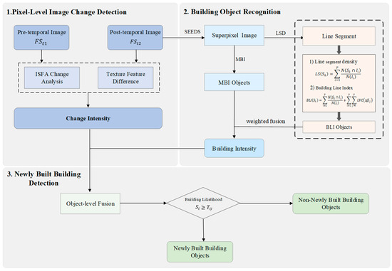
Figure 1.
Flowchart of newly built building detection. LS (Line Segment Density), BLI (Building Line Index), and LVC (Line segment Verticality Criterion). All index values are normalized to the range [0, 1].
2.1. Seeds Segmentation
Superpixel segmentation groups adjacent pixels sharing similar spectral, textural, and brightness characteristics into distinct clusters, each termed a superpixel. In this study, the SEEDS algorithm [30] is used to segment remote sensing images to obtain superpixel. In order to make the number of superpixels closer to the actual number of objects in the image, the initial number of segmented superpixels is assigned first, followed by a gradual reduction in superpixel count through an iterative decay strategy. The number of pixels decays according to the following formula:
where n denotes the number of superpixels, γ is an exponential parameter set to 0.95, representing the number of iterations, N_based is the initial number of superpixels, and each iteration is a re-segmentation of the last segmentation result.
In this study, the initial number of superpixels was set to 2000, which was empirically determined to provide a suitable balance between segmentation granularity and computational efficiency for images. The iterative decay process was terminated after 10 iterations, as further iterations did not yield significant changes in superpixel topology. We observed that the segmentation results were relatively stable with respect to and the number of iterations; varying between 1500 and 2500 or the iteration count between 8 and 12 resulted in negligible differences in the final building extraction accuracy (IoU variation < 0.01). This suggests that the proposed framework is robust to moderate variations in superpixel segmentation parameters.
2.2. Pixel-Level Image Change Detection
Beyond exhibiting distinct spectral characteristics, buildings also demonstrate considerable diversity in their spatial arrangement and density. To accurately capture building change information within the imagery, this study extracts pixel-level change data derived from both spectral and textural features. The spectral difference is obtained using Iterative Slow Feature Analysis (ISFA), while the textural difference is calculated through direct differencing of the texture features. Subsequently, change intensity information for each feature is computed by calculating the vector distance based on the respective band-wise change information. Finally, the spectral and textural difference maps are fused to generate the pixel-level change intensity. The detailed pixel-level change detection process comprises the following steps.
- Feature Difference Analysis
In this study, the Gray Level Co-occurrence Matrix (GLCM) is used to describe the texture features of buildings in the image, and the variance measure of the GLCM is used as the texture feature to extract the change information [31]. The GLCM was computed at the pixel level using a sliding window of size 9 × 9 pixels. The original image was quantized to 8 bits (256 gray levels). Four directions (0°, 45°, 90°, and 135°) with a pixel offset distance (d) of 1 were used, and the final texture feature for each pixel was obtained by averaging the variance values over these four directions to ensure rotational invariance. The calculation formula is as follows:
where represents the probability of occurrence of gray levels i and j in the given direction and distance d, is the mean of GLCM, and N represents the gray level.
The difference information of texture features is calculated by the weighted difference method, and the calculation formula is as follows:
where and are the normalized texture features of the bi-temporal images respectively, DT represents the difference result map of bi-temporal texture features, consisting of four bands (, , , ). t1 and t2 respectively refer to the time before and after the change detection, and w is the weight, which is calculated from the texture features of the two periods.
In order to analyze the change information of spectral features, this study adopts Iterative Slow Feature Analysis (ISFA) [32], which uses iterative weighting to learn the optimal slow feature space based on Slow Feature Analysis (SFA). The ISFA is implemented with the following parameters: the input data is first whitened, and all four slow features (equal to the number of input spectral bands) are retained. The iterative weighting process is run for 10 iterations, following the setup in [32]. After inputting the bi-temporal multispectral images, the characteristic difference is calculated as follows:
where DS is the characteristic difference of slow feature analysis. There are four bands, DS1, DS2, DS3, and DS4, which correspond to the change information of each band. ISFA is the iterative slow feature analysis operation, and and are the spectral characteristics of the two periods.
- Change Intensity Calculation
In order to obtain the final change intensity of spectral and texture features, a scatter plot is used to show the relationships between features. Figure 2 presents a scatter plot of the first two bands of DS and DT. In the scatter plot, a color gradient is used to represent the density of the scatter points, with red to purple representing the decrease in point density.
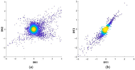
Figure 2.
Spectral and texture feature difference value scatter plot. (a) Spectral difference scatter plot. (b) Texture difference scatter plot.
The scatter plot between spectral feature difference bands shows a circular density distribution, while the texture feature difference bands have an elliptical distribution. This study uses Euclidean distance and Mahalanobis distance to calculate the intensity of spectral and texture feature changes, respectively. The formula is as follows:
where IS and IT represent the change intensities of spectral features and texture features, and and respectively represent the feature difference variable matrices. m is the mean of the texture feature difference, and S is the covariance matrix, represents the transpose operation, and represents the inversion operation.
In order to obtain the change intensity at the pixel level, this study fuses the spectrum and texture feature by summing. The calculation formula is as follows:
where F represents the normalization of the feature difference map, implemented as min-max normalization to scale the values to the range [0, 1]: , and CI represents the pixel-level change intensity. The larger the value, the greater the possibility of the position change.
2.3. Building Feature Extraction
2.3.1. Building Line Index
Since there are vertically intersecting line segments on the boundary of buildings, building features can be extracted by line segments. The main calculation process is as follows:
- Line Segment Density
After the line segment is extracted by the LSD (Line Segment Detector) [33] algorithm, when there are p line segments intersecting the superpixel , the line segment density is defined as
where represents the line segment density, and N() represents the number of pixels in the line segment. The more line segments that intersect with the superpixel, and the larger the proportion of line segments within the superpixel, the greater the line segment density value of the superpixel.
- 2.
- Line Segment Vertical Function
Due to the resolution of remote sensing images and the influence of terrain, it is difficult to achieve the condition where two adjacent sides of a building are completely vertical. Therefore, an allowable error of the inclination angle difference is introduced. In this study, the value of was set to 4 degrees. In order to assign different weights to the vertical line segments under different errors, functions based on the difference in inclination angle are introduced to represent the verticality of the line segments. The expressions are as follows:
where represents the verticality function of the line segments and , respectively, and the value range is 0:1. The larger the value, the greater the possibility that the line segments are perpendicular to each other.
Line segments intersecting each superpixel were clipped to the superpixel boundary before computing segment length and intersection angles. Short segments with fewer than 5 pixels were filtered out to avoid unstable angle estimates using the built-in filtering mechanism of the LSD algorithm. A graph of line segment vertical function is shown in Figure 3. The maximum value of the function is 1; the higher the value, the more vertical the line segments are.
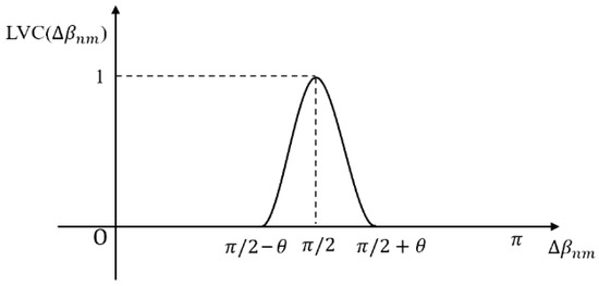
Figure 3.
Graph of line segment vertical function.
- 3.
- Building Line Index (BLI)
When line segments in the line segment set intersect with the superpixel , the BLI is calculated as follows:
where BLI is the building line index proposed in this study, p represents the number of line segments intersecting with superpixels, and represents the verticality of line segments and .
It is worth noting that while the line-constrained shape feature [27] also utilizes line segments to characterize building shapes, it primarily focuses on measuring the extension distance of vectors in multiple orientations before encountering line segments, thereby capturing object shape regularity. In contrast, the proposed BLI emphasizes the structural relationship among line segments—specifically, their density and perpendicularity—to better characterize building boundaries. Moreover, BLI is designed as a standalone building index that can be directly fused with spectral–spatial indices like MBI at the feature level, enabling unsupervised building extraction without relying on supervised classification or complex vector extension mechanisms.
2.3.2. Building Detection Using Fused BLI and MBI Features
Buildings exhibit distinct spectral–spatial characteristics in remote sensing imagery, primarily characterized by high reflectance values on rooftops and pronounced contrast with adjacent shadow areas. Additionally, building contours typically demonstrate relative regularity, with boundaries displaying specific spatial geometric relationships. To comprehensively incorporate both aspects of these features, this study employs a fusion of the MBI [34] and the BLI for building information extraction. The MBI primarily leverages spectral–spatial information features inherent to buildings. Conversely, the BLI, introduced in this study, focuses on boundary line segment characteristics of buildings. It further quantifies line segment density and spatial relationships to enhance building signatures. For buildings within the post-temporal imagery, the following extraction steps are implemented.
- 4.
- Image Segmentation
This study mainly extracts newly built buildings, and only performs superpixel segmentation on post-temporal images. Let the segmented image be denoted as OB, then its expression is
where represents the p-th superpixel.
- 5.
- Calculating Object-Level Building Features
Based on the superpixel, the BLI and MBI at the object level are calculated respectively, that is, the mean value of the feature in the superpixel is calculated. The calculation expression is
where , represents the average value of building index I based on segmented image OB, and is the average value of building index I based on superpixel , i = 1,2,3,…,p. The calculation formula is as follows:
where is the pixel value at of the building index, n and m represent the length and width of the rectangle with the same area as the superpixel , respectively.
- 6.
- Feature Fusion
In this study, Building Intensity (BI) is defined to represent the possibility that whether pixel is building, which is obtained by the weighted fusion of the BLI and MBI. The calculation formula is as follows:
where is an adjustable weighting factor, and F() represents the normalization of the building index. BI is a building index defined on the superpixel, which fuses information about the structure and spectrum of building. The larger the value, the greater the possibility that the pixel is a building.
2.4. Newly Built Building Recognition
Based on the newly built building detection framework proposed in this study, the pixels that meet the following two conditions can be considered as newly built buildings: (1) the superpixel changed between the two phases; (2) the superpixel is categorized as a building in the post-period. Firstly, the change detection results and post-temporal building information are fused to obtain the intensity map of newly built buildings. Then, a threshold is selected to distinguish newly built buildings and non-newly built buildings.
In order to achieve object-level feature fusion, it is necessary to convert the pixel-level change detection results to object-level results, denoting the transformed object-level change information as , expressed as follows:
In order to balance the change detection result and the post-temporal Building Intensity (BI), the following formula is used to calculate the newly built building information.
where NBI is the newly built buildings index, and F() is the feature normalization function.
is the threshold value of the NBI to assess newly built buildings. The calculation method is as follows:
where ms and std represent the mean and standard deviation of the NBI, and a is the adjustment factor, which was taken as 1.5 in this study.
Finally, based on the of the superpixel, it is possible to assess whether it represents a newly built building. The assessment criteria are as follows:
where is a threshold determined based on the likelihood of newly built buildings, and NB represents the final newly built building extraction results. A pixel gray value of 1 represents newly built buildings, and a pixel value of 0 represents the background.
Since roads and buildings have similar features, they will be extracted, but roads are longer, and their aspect ratios are very different from those of buildings. In this study, the geometric shape index (GI) is used as the evaluation index to filter superpixels with large aspect ratios, such as roads. The calculation formula is as follows:
where GI represents the geometric shape index, which is a feature calculated based on the connected domain, P represents the perimeter of the connected domain, and A represents the area of the connected domain. The larger the aspect ratio of the superpixel, the larger the GI value.
2.5. Evaluation Criteria
In order to more accurately evaluate the effectiveness of the newly built building detection methods in this study, a quantitative evaluation index is introduced. According to the parameter statistics of the confusion matrix, the following accuracy evaluation indexes are used:
where TP and FP are the numbers of newly built building pixels detected correctly and incorrectly, respectively, FN refers to the number of incorrectly detected non-newly built building pixels, and TN is the number of correctly detected non-newly built building pixels. PA is the pixel accuracy rate, which refers to the percentage of correctly detected pixels in all pixels in the image. MPA is the average pixel accuracy rate, which is the average value of the model’s detection accuracy for each category. IoU is the intersection over union, which is a comprehensive indicator of the detection accuracy and omission of newly built buildings.
3. Data
To evaluate the effectiveness of the proposed method, bi-temporal ZY-3 remote sensing images acquired in 2012 and 2016 were utilized. The experimental data comprise multispectral imagery encompassing four bands (blue, green, red, and near-infrared). Following pan-sharpening, the resulting imagery exhibits a spatial resolution of 2.1 m and dimensions of 2147 × 1718 pixels. The study area is situated within the Dongxihu District of Wuhan City, covering approximately 16.3 km2. Significant land cover transformations, particularly concerning buildings, occurred within this area between 2012 and 2016 due to urbanization processes.
Given the susceptibility of change detection accuracy to bi-temporal image quality, polynomial transformation [35] and a pseudo-invariant feature (PIF) method were applied to perform image registration and relative radiometric correction, respectively. Image registration was performed using a second-order polynomial transformation. Twelve control points were uniformly selected across the image to compute the transformation model. The registration error, evaluated using the Root Mean Square Error (RMSE) calculated over these control points, was confirmed to be less than one pixel (2.1 m). PIFs (e.g., stable asphalt roads and concrete surfaces) were manually selected based on their spectral stability and minimal change between the two temporal images. Linear regression was then applied based on these PIFs to normalize the radiometric differences. Outliers in the PIF set were identified and rejected during the regression process by applying a threshold to the residuals to ensure a robust correction model. This preprocessing ensured registration errors remained within one pixel. Figure 4a,b present true-color composites of the study area for 2012 and 2016, respectively. Figure 4c displays the manually delineated reference data used for accuracy assessment, where newly built buildings are represented in white against a black background.
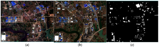
Figure 4.
Experimental remote sensing images. (a) A true color image from May 2012. (b) A true color image from August 2016. (c) Newly built buildings reference map.
4. Results
Figure 5 presents the study area imagery alongside the newly built building detection results. Specifically, Figure 5c depicts the resulting map of newly built buildings extracted by the proposed method, where detected buildings are represented in white against a black background. The study area, located in a suburban zone undergoing active urbanization, features predominantly large factories, commercial complexes, and high-rise residential developments as the main newly built structures. The proposed method demonstrates effectiveness in extracting these building types (e.g., large structures in regions Figure 5d–h; complex building clusters in regions Figure 5f,i; residential areas in region Figure 5g) by leveraging texture, spectral change information, and building-specific features within the corresponding regions. While large and well-lit buildings are reliably detected, the method exhibits limitations in capturing small and dark buildings, attributed to their lower response to the utilized building features. Crucially, the method successfully suppresses irrelevant objects, such as newly constructed roads (adjacent to region h), unchanged buildings, water bodies, farmland, and rivers, as the selected features primarily target building characteristics.
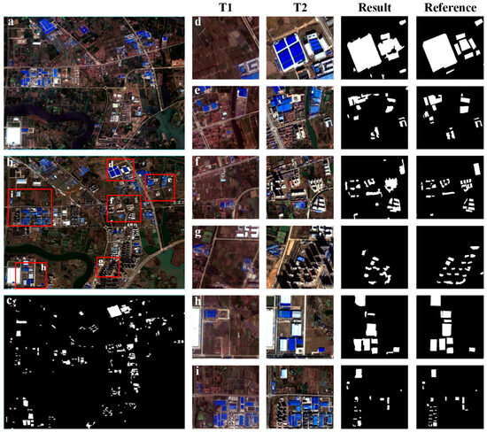
Figure 5.
Newly built building detection results. (a,b) Remote sensing images of the study area in 2012 and 2016, respectively. (c) Prediction results obtained by the method proposed. The spatial extents of regions (d–i) are the zoomed-in areas (red rectangles) of image (b). The last four columns show two remote sensing images (T1 is a 2012 image, T2 is a 2016 image), prediction results, and reference results.
4.1. Quantitative Evaluation
Quantitative evaluation at the pixel level was performed using the prediction results and the reference map. Key metrics include Pixel Accuracy (PA = 97.4%), Mean Pixel Accuracy (MPA = 83.6%), and Intersection over Union (IoU = 0.515) for newly built buildings. An IoU value exceeding 0.5 substantiates the effectiveness of the proposed method. Furthermore, high PA and MPA values indicate strong accuracy in extracting newly built buildings. Additionally, the pixel-level precision (0.686), recall (0.693), and F1-score (0.689) for newly built buildings were closely aligned, indicating a robust and balanced detection capability.
Beyond pixel-level assessment, object-level evaluation was conducted to better reflect practical performance. An object was considered correctly detected (True Positive) if its Intersection Over Union (IoU) with a reference building polygon exceeded 0.5. Based on this criterion, the object-level precision, recall, and F1-score were calculated. The results demonstrate exceptional performance, with values of 0.942, 0.881, and 0.91, respectively.
4.2. Performance Analysis Across Building Types
To systematically quantify the performance variation, reference buildings were stratified into three groups based on footprint area (small: <500 m2; medium: 500–2000 m2; large: >2000 m2) and into two groups based on average radiance in the NIR band (dark: bottom 30%; bright: top 70%). The object-level precision, recall and F1-score were computed for each group (Table 1).

Table 1.
Object-level accuracy across different building types.
The results clearly demonstrate that the method achieves higher accuracy for larger and brighter buildings, while performance on small and dark structures requires further improvement. Large buildings (>2000 m2) attained the highest F1-score of 0.941, significantly outperforming small buildings (<500 m2), which scored only 0.774 due to substantial omissions (recall = 0.715). Similarly, bright buildings demonstrated superior performance (F1 = 0.925) compared to dark buildings (F1 = 0.860). This analysis objectively identifies the current limitations and directs future research focus toward improving the detection of small and spectrally dark structures.
5. Discussion
The proposed framework for newly built building detection was evaluated using bi-temporal high-resolution remote sensing imagery, encompassing three core components: pixel-level change detection, post-temporal building extraction, and newly built building recognition. This section discusses (1) the impacts of likelihood threshold and geometric shape index on detection performance; (2) the effects of different feature fusion strategies; and (3) comparative analysis against existing methods.
5.1. Sensitivity Analysis
- (1)
- Analysis of Likelihood Threshold
In order to obtain the final newly built buildings, the likelihood map needs to be binarized. Therefore, the selection of the threshold will affect the extraction accuracy of the newly built buildings. Figure 6a shows the variation in accuracy of newly built buildings with different likelihood thresholds . PA and MPA are the accuracy indicators of two categories of newly built buildings and non-newly built buildings. They increase with the increase in , reflecting the accuracy of newly built buildings, but they lack statistics on omission. The IoU is an index to comprehensively measure the extraction effect of newly built buildings. When the likelihood threshold gradually increases, the IoU value increases first and then decreases. Figure 6b explains the influence of on the accuracy IoU of newly built buildings in more detail. The IoU provides comprehensive accuracy statistics of the recall and precision of newly built buildings. When the difference between recall and precision gradually becomes equal, IoU reaches the maximum; when the difference increases, the IoU begins to decrease.
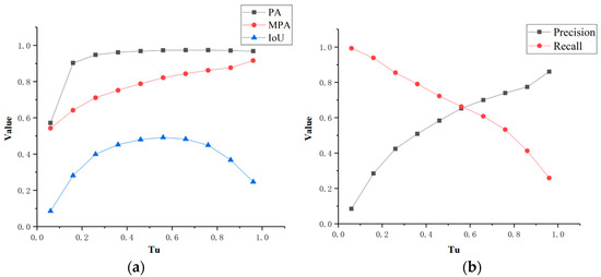
Figure 6.
Influence of likelihood threshold on the accuracy of newly built buildings. (a) Influence of likelihood threshold on the PA, MPA, and IoU. (b) Influence of likelihood threshold on recall and precision.
- (2)
- Sensitivity analysis of angle tolerance
A sensitivity analysis was conducted to evaluate the impact of the angle tolerance parameter in the Line segment Verticality Criterion (LVC) function on pixel-level detection accuracy (with the fusion weight fixed at 0.4). The results, summarized in Table 2, reveal a clear non-linear relationship between angular tolerance and detection performance.
Table 2.
Sensitivity analysis of angle tolerance on pixel-level detection accuracy ( = 0.4).
The analysis reveals that = 4° provides the optimal balance for building detection, achieving the highest F1-score of 0.689 with well-matched precision (0.692) and recall (0.683). This specific tolerance value appears to offer the ideal compromise, enabling effective identification of characteristic building perpendicularity while minimizing both false positives and omissions.
When θ was reduced below this optimum < 4°), performance deteriorated significantly due to severely constrained recall. At = 0°, recall dropped sharply to 0.402, reducing the F1-score to 0.522 despite relatively high precision. This confirms that excessively strict angular criteria cannot adequately capture the near-vertical line segments commonly present in actual building imagery. Notably, when increased to 5°, the F1-score already showed a slight decline to 0.682, indicating that the optimal performance window is relatively narrow. As the tolerance broadened further ( > 5°), a progressive performance decline was observed, with the F1-score dropping to 0.670 at = 6° and continuing to decrease with expanding tolerance. This pattern emerged because increasingly wider angular windows incorporated more non-orthogonal line segments from non-building features, systematically reducing precision while recall also gradually diminished.
This analysis validates = 4° as the optimal parameter setting for the LVC function, providing the most effective balance for utilizing perpendicular line segments as discriminative structural features in building detection at the pixel level.
- (3)
- Sensitivity analysis of adjustable parameters
To assess the impact of the fusion weight between the Building Line Index (BLI) and the Morphological Building Index (MBI), a sensitivity analysis was conducted with the angle tolerance fixed at its optimal value ( = 4°). The parameter , which ranges from 0 to 1, controls the relative contribution of the structural feature (BLI) and the spectral–spatial feature (MBI) in the fused Building Intensity (BI), as defined in Equation (14). The pixel-level detection accuracy under different φ values is summarized in Table 3.
Table 3.
Sensitivity analysis of the fusion weight on pixel-level detection accuracy ( = 4°).
The results demonstrate that the proposed fusion strategy is crucial for achieving optimal performance, with the highest F1-score of 0.689 achieved at = 0.4. This balanced weighting allowed for an effective integration of the high precision characteristic of the MBI and the high recall characteristic of the BLI.
When = 0 (relying solely on the MBI), the model maintained a relatively high F1-score of 0.673, with high precision (0.721) but moderate recall (0.630). This indicates that while the MBI alone provides reliable detection of clear building signatures, it remains conservative and misses a substantial number of true positives, particularly buildings with weak spectral–spatial responses. Conversely, when = 1.0 (relying solely on the BLI), the model achieved the highest recall (0.758) but suffered from the lowest precision (0.592), resulting in a lower F1-score of 0.665. This pattern confirms that the structural feature BLI, while highly sensitive in identifying potential building pixels, introduces significant false alarms from non-building objects with linear structures when used without spectral–spatial constraints.
The performance plateau observed for φ values between 0.2 and 0.6 (F1-score > 0.683) indicates robustness in the fusion framework. However, the clear peak at = 0.4 validates that a balanced contribution from both structural (BLI) and spectral–spatial (MBI) features is superior to relying on either feature type alone. The empirically determined value of = 0.4 was therefore adopted for all other experiments in this study.
- (4)
- Ablation Study on Change Intensity (CI) Components
An ablation study was conducted to evaluate the individual contribution of the spectral and textural features to the final pixel-level change detection result. The Change Intensity (CI) map, a key input to the framework (Equation (7)), was computed under three different configurations while keeping all other parameters ( = 4°, = 0.4, likelihood threshold) at their optimal values. The pixel-level accuracy for detecting newly built buildings under each configuration is presented in Table 4.
Table 4.
Ablation study on the composition of the Change Intensity (CI).
The results clearly demonstrate the effectiveness of the proposed feature fusion strategy. Employing the combined CI map (ISFA + Texture) yielded the highest overall performance, achieving a balanced F1-score of 0.689.
The ISFA-only configuration exhibited a higher recall (0.705) but notably lower precision (0.662), resulting in a lower F1-score (0.683). This pattern suggests that spectral change information is highly sensitive in identifying potential changes but is less specific to building-related changes, leading to more false alarms from phenomena like vegetation growth or soil moisture variation. Conversely, the texture-only configuration showed the opposite trend, achieving the highest precision (0.698) among the three but the lowest recall (0.645). This indicates that textural change is a more specific indicator for structured objects like buildings, effectively suppressing some false alarms. However, it fails to capture all relevant building changes, especially those with less pronounced textural variation, resulting in significant under-detection.
The fusion of both features successfully mitigates the individual weaknesses of each. The combined approach balances the high sensitivity of the spectral feature with the high specificity of the textural feature, achieving a superior trade-off between false positives (precision) and false negatives (recall). This ablation study validates the design choice of integrating both spectral and textural information at the pixel-level change detection stage, confirming that their synergistic combination is crucial for the framework’s high performance.
- (5)
- Analysis of GI
Table 5 shows the accuracy change of the newly built buildings after filtering by GI. It can be found that the improvement for PA is small, and the MPA and IoU values are 0.017 and 0.023, respectively. The improvement of the IoU value indicates that the overall accuracy of newly built building detection has improved, which verifies the effectiveness of GI in this study. The main purpose of introducing GI is to filter some false alarms with extremely large aspect ratios, thereby improving the detection accuracy of newly built buildings. In this experiment, the detection accuracy of newly built buildings increased by 0.031.
Table 5.
Accuracy improvement of GI optimization.
5.2. Analysis of Different Decision Fusion Methods
To evaluate the discriminative performance of the Building Intensity (BI) and Change Intensity (CI) features across major land-cover classes, representative sample points were selected for Newly Built Buildings (NBs), Unchanged Buildings (UCBs), and Other Land (including water bodies, roads, farmland) within the study area (Figure 7c). Figure 7a,b depict the CI map and post-temporal BI map, respectively, generated by our method. Regions exhibiting high intensity values in both maps correspond to areas with a high likelihood of being newly built buildings.
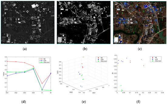
Figure 7.
Performance of BI and CI on the main land-cover classes: (a) change intensity (CI); (b) post-temporal building intensity (BI); (c) sampling point location (red for NB, yellow for UCB, green for other land); (d) line chart of main land-cover classes for different features; (e) scatter plot of main land-cover classes for spectral features; (f) scatter plot of main land-cover classes for BI and CI.
Figure 7d presents the mean feature values for each land-cover class across the different feature maps. Analysis reveals that NB samples consistently demonstrate higher values in both BI and CI features compared to UCBs and Other Land. Furthermore, NB samples exhibit significantly higher spectral feature differences (DS), particularly in the first three bands. In contrast, UCB samples show lower CI values but BI values comparable to NB samples. Other Land samples consistently display low values for both BI and CI features.
Figure 7e,f visualize the spatial distribution of these land-cover classes within the spectral difference (DS) feature space and the combined BI-CI feature space, respectively. The BI-CI feature space demonstrates superior class separability, effectively distinguishing NBs from other land-cover classes compared to the DS feature space. These results collectively indicate that the BI and CI features employed in this study provide enhanced discriminative power for the extraction of newly built buildings.
In the proposed framework for newly built building extraction, the final result is derived through the fusion of pixel-level change detection and object-level building information. To investigate the impact of the fusion strategy on the outcome, comparative experiments were conducted, evaluating both single-feature performance and an alternative decision-level fusion approach [36]. This study employed feature-level fusion. For comparison, the decision-level fusion method involves separately binarizing the two features and subsequently combining them through logical operations to obtain the final fused result.
Figure 8 provides a visual comparison of the results obtained using decision-level fusion versus feature-level fusion. Specifically, Figure 8a,b depict scatter plots within the spectral difference space, comparing the newly built building results from each fusion method against the reference data. While both sets of results exhibit some similarity, the point cloud representing the decision-level fusion result demonstrates a more pronounced deviation from the reference point set. Figure 8c overlays the newly built building detection results from both fusion methods with the reference map. Analysis of this figure reveals that the decision-level fusion results contain a higher prevalence of false alarms (depicted by blue areas in Figure 8c). Furthermore, the presence of yellow patches indicates that the decision-level fusion approach exhibits greater omission errors compared to the feature-level method. Notably, the scarcity of pink patches suggests that the feature-level fusion method achieves superior detection completeness with fewer omissions.
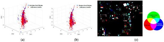
Figure 8.
Comparison of decision-level fusion and feature-level fusion: (a) spectral feature scatter plot of decision-level fusion; (b) spectral feature scatter plot of feature-level fusion; (c) comparison of fusion results of different methods.
Figure 9 quantitatively compares the accuracy achieved using the individual features (BI and CI, representing post-temporal building intensity and change intensity, respectively) and the two fusion methods. The single-feature comparison clearly indicates that CI yields significantly higher accuracy than BI. This discrepancy primarily arises because BI solely captures building presence in the post-temporal image and lacks explicit change information. Furthermore, the decision-level fusion method exhibits slightly lower accuracy than the feature-level fusion approach adopted in this study. This performance difference is largely attributable to the requirement in decision-level fusion to independently threshold each feature before performing the logical intersection operation. This multi-step process inherently introduces potential errors, leading to an increase in false alarms and consequently reducing overall extraction accuracy.
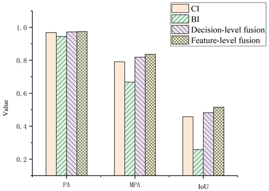
Figure 9.
Comparison of different fusion methods, showing a quantitative evaluation of the accuracy achieved using the individual features (BI and CI, representing post-temporal building intensity and change intensity, respectively) and the two fusion methods. The quantitative results (PA: 0.968, 0.944, 0.972, 0.974; MPA: 0.791, 0.668, 0.819, 0.836; IoU: 0.457, 0.258, 0.482, 0.515 for CI, BI, decision-level, and feature-level fusion, respectively) demonstrate that the feature-level fusion strategy outperforms both single-feature approaches and decision-level fusion, achieving the best overall accuracy.
5.3. Experiments Compared to Other Methods
As an unsupervised technique aimed at practical applications with limited labeled data, the performance of the proposed method was assessed by comparing it with three established unsupervised building change detection approaches. (1) OBISFA: This method builds upon ISFA by incorporating an object-oriented processing step, where the mean ISFA value within each object serves as the detection result. (2) SFAMBI: The difference fusion of SFA and MBI features is used to extract the change information. Three fusion methods were used in article [37], and the weighted fusion method was used in the comparison experiment in this paper. (3) SPETEXMBI: As described in [38], this method utilizes spectral and texture features to derive multi-temporal change information, subsequently applying MBI change information to filter out building change objects.
Figure 10 visually compares the newly built building extraction results from the different methods. In the figure, green denotes results from the proposed method, red represents the reference data (ground truth), and blue indicates results from the alternative method being compared in each sub-figure. Figure 10a compares the proposed method with OBISFA. A higher prevalence of blue patches (e.g., in Region 1) indicates that OBISFA produces more false alarms. Figure 10b compares the proposed method with SFAMBI. Similarly, this sub-figure shows numerous blue patches, signifying false alarms, alongside omissions (e.g., in Regions 2 and 3). Figure 10c presents the comparison with SPETEXMBI. Here, a large number of yellow patches are evident, highlighting substantial omissions in the SPETEXMBI results, particularly in large-scale industrial areas (e.g., Region 4). Conversely, the scarcity of blue patches in Figure 10c suggests SPETEXMBI generates fewer false alarms. Across all sub-figures, green, yellow, and white patches predominate, visually demonstrating the superior detection performance of the proposed framework compared to the three alternative methods.
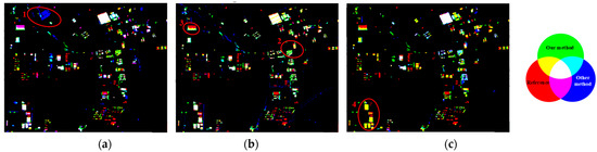
Figure 10.
Results of newly built buildings extracted by different methods: (a) Blue shows the results of OBISFA, red shows reference results, green shows the results of our method; (b) blue shows the results of SFAMBI, red shows reference results, green shows the results of our methods; (c) blue shows the results of SPETEXMBI, red shows reference results, green shows the results of our method.
To qualitatively assess the differences in newly built building extraction across the evaluated methods, scatter plots were generated in both the spectral and texture feature spaces. Figure 11 presents these scatter plots for the four algorithms, where blue points represent the extracted results for each method and red points represent the reference data. Each point corresponds to the mean spectral or texture feature difference value calculated for an individual object within the respective extraction results.
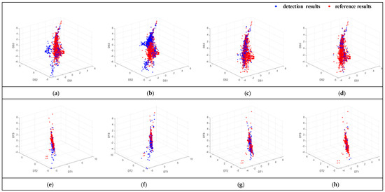
Figure 11.
Scatter plots of texture and spectral features for different methods: (a) spectral feature scatter plot of OBISFA; (b) spectral feature scatter plot of SFAMBI; (c) spectral feature scatter plot of SPETEXMBI; (d) spectral feature scatter plot of our method; (e) texture feature scatter plot of OBISFA; (f) texture feature scatter plot of SFAMBI; (g) texture feature scatter plot of SPETEXMBI; (h) texture feature scatter plot of our method. The centroid distances between the extracted results and the reference data are provided as a quantitative measure of this agreement: OBISFA (spectral: 0.922; texture: 0.392), SFAMBI (spectral: 1.546; texture: 0.328), SPETEXMBI (spectral: 0.209; texture: 0.581), and our method (spectral: 0.182; texture: 0.145).
The degree of spatial overlap between the blue (method result) and red (reference) point sets within these feature spaces serves as an indicator of extraction accuracy; greater overlap signifies closer alignment between the method’s output and the ground truth. Visual inspection of Figure 11 reveals distinct spatial distributions for the different methods. Notably, the scatter points associated with spectral features exhibit relatively dispersed distributions, while those for texture features appear more concentrated. Crucially, the scatter plots for OBISFA, SFAMBI, and SPETEXMBI demonstrate visibly lower overlap with the reference data points compared to the proposed method.
To quantitatively characterize this spatial overlap, the centroid distance between each method’s scatter set and the reference scatter set was computed. A smaller centroid distance indicates a higher degree of spatial overlap and thus better agreement with the reference data. As shown in Table 6, the proposed method achieves the smallest centroid distance for both feature spaces. This combined qualitative (visual overlap) and quantitative (centroid distance) analysis demonstrates that the extraction results produced by the proposed method exhibit the closest alignment with the reference results.
Table 6.
The centroid distances of scatter between the predicted results and the reference results by different methods.
The accuracy of the SPETEXMBI method was the lowest. The main reason is that the method involves the threshold selection and logical operation of multiple features, which brings a lot of uncertainty to the extracted results and increases the proportion of false alarms. At the same time, the method detects spectral and texture changes using direct differencing, which leads to many noise points in the results and reduces precision.
Figure 12 presents the newly built building extraction accuracy results across all comparative experiments. The results demonstrate that the method proposed in this study achieved the highest accuracy performance. OBISFA exhibited superior accuracy compared to the other two benchmark methods, attributed to its utilization of iterative weighting within ISFA, which enhances its effectiveness over the basic SFA approach. Conversely, the SPETEXMBI method yielded the lowest accuracy. This is primarily due to its reliance on threshold selection and logical operations for multiple features, introducing significant uncertainty into the extracted results and elevating the proportion of false alarms. Furthermore, SPETEXMBI’s reliance on direct differencing for spectral and texture change detection contributes to the presence of noise in the results, thereby reducing precision.
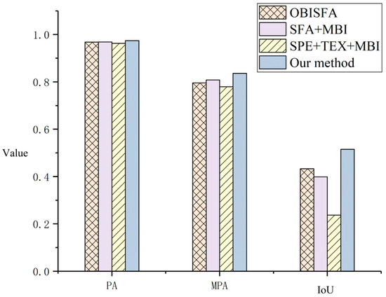
Figure 12.
Accuracy comparison of different newly built building detection methods. The quantitative results are as follows: OBISFA (PA: 0.968, MPA: 0.796, IoU: 0.433), SFAMBI (PA: 0.969, MPA: 0.808, IoU: 0.399), SPETEXMBI (PA: 0.963, MPA: 0.779, IoU: 0.237). The proposed method achieved the highest scores across all metrics, with a PA of 0.974, MPA of 0.836, and IoU of 0.515.
6. Conclusions
This study proposed a novel BLI for extracting buildings based on line segment features and introduced an unsupervised framework for detecting newly built buildings by integrating pixel-level change information with object-level building features. Under this framework, we achieved a pixel accuracy of 0.974, an average class accuracy of 0.836, and an Intersection over Union (IoU) for newly built buildings of 0.515. Critically, at the object-level, which better reflects practical utility, the method achieved high precision of 0.942, recall of 0.881, and an F1-score of 0.91. The research findings offer valuable insights from both conceptual and practical perspectives.
- Conceptual Implications
This work makes several key theoretical contributions to the field of remote sensing change detection. Firstly, it introduces BLI, a novel building-specific index that innovatively leverages the density and perpendicularity of line segments to characterize building structural boundaries, moving beyond traditional spectral or simple geometric features. Secondly, it presents a robust unsupervised technical framework that effectively integrates pixel-level change detection with object-level, mono-temporal building information at the feature level. This approach demonstrates how change information and building characteristics can be synergistically combined without relying on manually labeled samples, advancing methodological knowledge in unsupervised analysis. Furthermore, the comparative analysis confirms that the proposed feature-level fusion strategy outperforms both single-feature extraction and decision-level fusion, providing a significant conceptual advancement in fusion techniques for change detection.
- Practical Implications
The proposed method has direct and meaningful applications in real-world scenarios. It provides an essential technical pathway for the automatic and efficient monitoring of urban land resources, supporting timely and accurate updates of building inventories. This capability is crucial for urban planning, cadastral management, and monitoring urban sprawl. For practitioners in government and environmental agencies, this tool can aid in tracking compliance with land-use policies, assessing the impact of urbanization on ecosystems, and informing sustainable development strategies. The unsupervised nature of the framework makes it particularly valuable for applications in areas where labeled training data are scarce or unavailable, thereby lowering the barrier for widespread adoption and enabling large-scale, operational monitoring of construction activities.
- Future Work
Notwithstanding its promising results, this study has certain limitations that point to valuable future research directions. First, the framework’s performance relies on precise image registration and radiometric normalization, as inaccuracies can introduce noise in change detection. Second, the dependence on handcrafted features (BLI and MBI) leads to difficulties in reliably detecting small and spectrally dark buildings. Finally, the evaluation was based on a single case study, which limits the generalizability of the findings across diverse regions and urban contexts. Future research will focus on validating and enhancing the robustness of the framework by applying it to diverse geographic environments, varying urban morphological contexts, and multi-temporal remote sensing data from different sensors. This will further verify the method’s adaptability and scalability across regions and complex scenarios. Additionally, we will explore the integration of unsupervised strategies with deep learning in semi-supervised settings, leveraging the strengths of both approaches to improve performance while maintaining applicability in label-scarce scenarios.
Author Contributions
Conceptualization, X.C.; methodology, X.C.; software, X.C. and H.X.; validation, H.X. and Z.Y.; formal analysis, M.W.; investigation, G.W.; data curation, M.W.; writing—original draft preparation, X.C. and M.W.; writing—review and editing, X.C., G.W. and J.C.; visualization, X.C. All authors have read and agreed to the published version of the manuscript.
Funding
This research was funded by the National Natural Science Foundation of China, grant number U22B2011.
Data Availability Statement
The dataset of the Dongxihu District, including a representative image crop and the corresponding manual reference masks for sanity checks, will be made publicly available upon acceptance of this manuscript on GitHub.
Conflicts of Interest
The authors declare no conflicts of interest.
Nomenclature
| Symbol | Description | SI Units |
| Building Line Index | Dimensionless | |
| Line Segment Density | Dimensionless | |
| Angle tolerance in LVC | Radians (rad) | |
| Change Intensity | Dimensionless | |
| Spectral Change Intensity | Dimensionless | |
| Texture Change Intensity | Dimensionless | |
| Building Intensity | Dimensionless | |
| Newly Built Building Index | Dimensionless | |
| Decision Threshold | Dimensionless | |
| Geometric Shape Index | Dimensionless | |
| Perimeter of a connected domain | Meters (m) | |
| Area of a connected domain | Square meters (m2) | |
| Fusion weight between BLI and MBI | Dimensionless |
References
- Guo, H.; Shi, Q.; Marinoni, A.; Du, B.; Zhang, L. Deep building footprint update network: A semi-supervised method for updating existing building footprint from bi-temporal remote sensing images. Remote Sens. Environ. 2021, 264, 112589. [Google Scholar] [CrossRef]
- Huang, X.; Cao, Y.; Li, J. An automatic change detection method for monitoring newly constructed building areas using time-series multi-view high-resolution optical satellite images. Remote Sens. Environ. 2020, 244, 111802. [Google Scholar] [CrossRef]
- Bai, Y.; Jiang, B.; Wang, M.; Li, H.; Alatalo, J.M.; Huang, S. New ecological redline policy (ERP) to secure ecosystem services in China. Land Use Policy 2016, 55, 348–351. [Google Scholar] [CrossRef]
- Kong, X. China must protect high-quality arable land. Nature 2014, 506, 7. [Google Scholar] [CrossRef] [PubMed]
- Zhang, Y.; Woodcock, C.E.; Arévalo, P.; Olofsson, P.; Tang, X.; Stanimirova, R.; Bullock, E.; Tarrio, K.R.; Zhu, Z.; Friedl, M.A. A Global Analysis of the Spatial and Temporal Variability of Usable Landsat Observations at the Pixel Scale. Front. Remote Sens. 2022, 3, 894618. [Google Scholar] [CrossRef]
- Lin, J.; Bo, W.; Dong, X.; Zhang, R.; Yan, J.; Chen, T. Evolution of vegetation cover and impacts of climate change and human activities in arid regions of Northwest China: A Mu Us Sandy Land case. Environ. Dev. Sustain. 2025, 27, 18977–18996. [Google Scholar] [CrossRef]
- Richardson, R.T.; Conflitti, I.M.; Labuschagne, R.S.; Hoover, S.E.; Currie, R.W.; Giovenazzo, P.; Guarna, M.M.; Pernal, S.F.; Foster, L.J.; Zayed, A. Land use changes associated with declining honey bee health across temperate North America. Environ. Res. Lett. 2023, 18, 064042. [Google Scholar] [CrossRef]
- Liang, X.; He, J.; Jin, X.; Zhang, X.; Liu, J.; Zhou, Y. A new framework for optimizing ecological conservation redline of China: A case from an environment-development conflict area. Sustain. Dev. 2024, 32, 1616–1633. [Google Scholar] [CrossRef]
- Jaturapitpornchai, R.; Matsuoka, M.; Kanemoto, N.; Kuzuoka, S.; Ito, R.; Nakamura, R. Newly built construction detection in SAR images using deep learning. Remote Sens. 2019, 11, 1444. [Google Scholar] [CrossRef]
- Li, Q.; Mou, L.; Sun, Y.; Hua, Y.; Shi, Y.; Zhu, X.X. A review of building extraction from remote sensing imagery: Geometrical structures and semantic attributes. IEEE Trans. Geosci. Remote Sens. 2024, 62, 1–15. [Google Scholar] [CrossRef]
- Huang, X.; Zhang, L.; Li, P. Classification and extraction of spatial features in urban areas using high-resolution multispectral imagery. IEEE Geosci. Remote Sens. Lett. 2007, 4, 260–264. [Google Scholar] [CrossRef]
- Falco, N.; Dalla Mura, M.; Bovolo, F.; Benediktsson, J.A.; Bruzzone, L. Change detection in VHR images based on morphological attribute profiles. IEEE Geosci. Remote Sens. Lett. 2012, 10, 636–640. [Google Scholar] [CrossRef]
- Collins, J.; Dronova, I. Urban Landscape Change Analysis Using Local Climate Zones and Object-Based Classification in the Salt Lake Metro Region, Utah, USA. Remote Sens. 2019, 11, 1615. [Google Scholar] [CrossRef]
- Wania, A.; Kemper, T.; Tiede, D.; Zeil, P. Mapping recent built-up area changes in the city of Harare with high resolution satellite imagery. Appl. Geogr. 2014, 46, 35–44. [Google Scholar] [CrossRef]
- Tian, J.; Cui, S.; Reinartz, P. Building change detection based on satellite stereo imagery and digital surface models. IEEE Trans. Geosci. Remote Sens. 2013, 52, 406–417. [Google Scholar] [CrossRef]
- Pang, S.; Hu, X.; Zhang, M.; Cai, Z.; Liu, F. Co-segmentation and superpixel-based graph cuts for building change detection from bi-temporal digital surface models and aerial images. Remote Sens. 2019, 11, 729. [Google Scholar] [CrossRef]
- Wu, J.; Ni, W.; Bian, H.; Cheng, K.; Liu, Q.; Kong, X.; Li, B. Unsupervised Change Detection for VHR Remote Sensing Images Based on Temporal-Spatial-Structural Graphs. Remote Sens. 2023, 15, 1770. [Google Scholar] [CrossRef]
- Ji, L.; Zhao, J.; Zhao, Z. A Novel End-to-End Unsupervised Change Detection Method with Self-Adaptive Superpixel Segmentation for SAR Images. Remote Sens. 2023, 15, 1724. [Google Scholar] [CrossRef]
- Li, W.; Li, Y.; Zhu, Y.; Wang, H. Unsupervised SAR Image Change Detection via Structure Feature-Based Self-Representation Learning. IEEE Trans. Geosci. Remote Sens. 2025, 63, 1–18. [Google Scholar] [CrossRef]
- Peng, D.; Zhang, Y. Building change detection by combining lidar data and ortho image. Int. Arch. Photogramm. Remote Sens. Spat. Inf. Sci. 2016, 41, 669–676. [Google Scholar] [CrossRef]
- Ullo, S.L.; Zarro, C.; Wojtowicz, K.; Meoli, G.; Focareta, M. LiDAR-based system and optical VHR data for building detection and mapping. Sensors 2020, 20, 1285. [Google Scholar] [CrossRef]
- Wei, D.; Yang, W. Detecting damaged buildings using a texture feature contribution index from post-earthquake remote sensing images. Remote Sens. Lett. 2020, 11, 127–136. [Google Scholar] [CrossRef]
- Gopinath, G.; Thodi, M.F.C.; Surendran, U.P.; Prem, P.; Parambil, J.N.; Alataway, A.; Al-Othman, A.A.; Dewidar, A.Z.; Mattar, M.A. Long-Term Shoreline and Islands Change Detection with Digital Shoreline Analysis Using RS Data and GIS. Water 2023, 15, 244. [Google Scholar] [CrossRef]
- Bagwan, W.A.; Sopan Gavali, R. Dam-triggered Land Use Land Cover change detection and comparison (transition matrix method) of Urmodi River Watershed of Maharashtra, India: A Remote Sensing and GIS approach. Geol. Ecol. Landsc. 2021, 7, 189–197. [Google Scholar] [CrossRef]
- Li, P.; Song, B.; Xu, H. Urban building damage detection from very high resolution imagery by One-Class SVM and shadow information. In Proceedings of the 2011 IEEE International Geoscience and Remote Sensing Symposium, Vancouver, BC, Canada, 24–29 July 2011; pp. 1409–1412. [Google Scholar]
- Schneider, A. Monitoring land cover change in urban and peri-urban areas using dense time stacks of Landsat satellite data and a data mining approach. Remote Sens. Environ. 2012, 124, 689–704. [Google Scholar] [CrossRef]
- Liu, H.; Yang, M.; Chen, J.; Hou, J.; Deng, M. Line-constrained shape feature for building change detection in VHR remote sensing imagery. ISPRS Int. J. Geo-Inf. 2018, 7, 410. [Google Scholar] [CrossRef]
- Tan, K.; Jin, X.; Plaza, A.; Wang, X.; Xiao, L.; Du, P. Automatic change detection in high-resolution remote sensing images by using a multiple classifier system and spectral–spatial features. IEEE J. Sel. Top. Appl. Earth Obs. Remote Sens. 2016, 9, 3439–3451. [Google Scholar] [CrossRef]
- Zhang, Y.; Peng, D.; Huang, X. Object-based change detection for VHR images based on multiscale uncertainty analysis. IEEE Geosci. Remote Sens. Lett. 2017, 15, 13–17. [Google Scholar] [CrossRef]
- Van den Bergh, M.; Boix, X.; Roig, G.; Van Gool, L. Seeds: Superpixels extracted via energy-driven sampling. Int. J. Comput. Vis. 2015, 111, 298–314. [Google Scholar] [CrossRef]
- Yogeshwari, M.; Thailambal, G. Automatic feature extraction and detection of plant leaf disease using GLCM features and convolutional neural networks. Mater. Today Proc. 2023, 81, 530–536. [Google Scholar] [CrossRef]
- Wu, C.; Du, B.; Zhang, L. Slow feature analysis for change detection in multispectral imagery. IEEE Trans. Geosci. Remote Sens. 2013, 52, 2858–2874. [Google Scholar] [CrossRef]
- Grompone von Gioi, R.; Jakubowicz, J.; Morel, J.-M.; Randall, G. LSD: A fast line segment detector with a false detection control. IEEE Trans. Pattern Anal. Mach. Intell. 2010, 32, 722–732. [Google Scholar] [CrossRef]
- Huang, X.; Zhang, L. Morphological building/shadow index for building extraction from high-resolution imagery over urban areas. IEEE J. Sel. Top. Appl. Earth Obs. Remote Sens. 2011, 5, 161–172. [Google Scholar] [CrossRef]
- Chen, G.; Zhao, K.; Powers, R. Assessment of the image misregistration effects on object-based change detection. ISPRS J. Photogramm. Remote Sens. 2014, 87, 19–27. [Google Scholar] [CrossRef]
- Huang, X.; Zhang, L.; Zhu, T. Building change detection from multitemporal high-resolution remotely sensed images based on a morphological building index. IEEE J. Sel. Top. Appl. Earth Obs. Remote Sens. 2013, 7, 105–115. [Google Scholar] [CrossRef]
- Huang, X.; Zhu, T.; Zhang, L.; Tang, Y. A novel building change index for automatic building change detection from high-resolution remote sensing imagery. Remote Sens. Lett. 2014, 5, 713–722. [Google Scholar] [CrossRef]
- Xiao, P.; Zhang, X.; Wang, D.; Yuan, M.; Feng, X.; Kelly, M. Change detection of built-up land: A framework of combining pixel-based detection and object-based recognition. ISPRS J. Photogramm. Remote Sens. 2016, 119, 402–414. [Google Scholar] [CrossRef]


Disclaimer/Publisher’s Note: The statements, opinions and data contained in all publications are solely those of the individual author(s) and contributor(s) and not of MDPI and/or the editor(s). MDPI and/or the editor(s) disclaim responsibility for any injury to people or property resulting from any ideas, methods, instructions or products referred to in the content. |
© 2025 by the authors. Licensee MDPI, Basel, Switzerland. This article is an open access article distributed under the terms and conditions of the Creative Commons Attribution (CC BY) license (https://creativecommons.org/licenses/by/4.0/).