Abstract
Increasingly stringent energy directives of the European Union, combined with rising cooling demands due to climate change, urge the investigation of energy-efficient cooling solutions. Free cooling offers a viable approach to reducing energy consumption. However, its effectiveness and applicability across different building types remain insufficiently established. This study aims to minimise mechanical cooling energy demand through the implementation of enhanced free cooling (EFC) as an operational control strategy in office, residential, and small commercial buildings. The introduction of the efficiency of EFC (ηfc) supports this analysis by quantifying how effectively EFC exploits free cooling potential in defined thermal and mechanical conditions based on an analytical approach supported by simplified simulations (in Microsoft Excel). The case study indicates that the east-oriented office building with a 40% glazing ratio achieves the highest cooling energy savings (49.63%) on the target summer day. For the residential building, savings are lower (37.78%) but more stable across the hot and the extremely hot days. The results further show that the influence of building orientation diminishes as external temperature increases, while higher glazing ratios stabilise ηfc across the examined thermal conditions. Analysis of the connection between air exchange rate and mechanical cooling energy savings identifies a critical resistance point (nopt), defined as the ventilation rate beyond which no further cooling energy savings occur. The results enable practical applications in building operation and support both improved energy efficiency and the advancement of sustainable HVAC design.
1. Introduction
1.1. Literature Review
The 2010/30/EU directive [1] has exerted significant influence on the energy-related development of buildings. It emphasises passive design strategies [2], such as enhanced thermal insulation [3] and increased glazed surface areas [4]. These methods primarily aim to reduce heating energy demand and heating degree-day (‘DDH’) values. As a result, the thermal characteristics of both new and retrofitted buildings have improved significantly [5]. This design approach, however, introduces secondary effects that received limited attention from regulators. Improved insulation and increased airtightness contribute to substantial heat accumulation within buildings in summer periods [6]. Cooling degree-day (‘DDC’) values rise across the European Union [7,8], driven by climate change and intensified indoor heat accumulation. In Hungary, this tendency is particularly pronounced: DDH values decline while DDC values increase significantly, as illustrated in Figure 1.
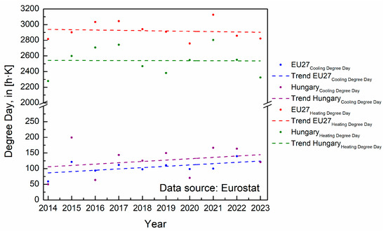
Figure 1.
Trends in annual Cooling Degree Days (DDC) and Heating Degree Days (DDH) in the EU and Hungary, 2014–2023 (Source: Eurostat; data processed and visualised by authors).
These shifts present new challenges for building HVAC systems, as cooling demand rises and access to higher comfort categories becomes more affordable—accelerating the proliferation of mechanical cooling solutions. The increasing prevalence of mechanical cooling contributes to the rising share of cooling systems within the energy balance of buildings [9]. This trend is particularly significant given that buildings account for over 60% of total energy consumption globally [10]. However, these mechanical cooling systems place considerable strain on the electricity grid, especially when peak-load conditions prevail. This strain contributes to increased energy production costs and destabilises the overall energy balance. Potential solutions to this issue can be explored at multiple levels (without claiming exhaustiveness):
- Country level: construction of new power generation facilities (e.g., nuclear power plants) [11];
- Urban level: Development of district cooling networks [12,13];
- Building level: Deployment of non-electric cooling technologies (e.g., absorption chillers) [14] or advanced energy storage systems (e.g., phase change material-based storage) [15,16];
- Operational level: Thermal insulation of HVAC systems [17] or adoption of optimised operational strategies [18]. This category also includes retrofitted passive and semi-active solutions, typically introduced as supplementary interventions beyond the original HVAC design.
The present study focuses on the latter group of interventions, as these typically require neither substantial financial investment nor extensive community coordination. Retrofitted passive solutions are also consistent with the principles of Directive 2010/30/EU [1]. This group incorporates the careful design and renovation of building envelopes [19], improved heat dissipation to the external environment [20], and the limitation of internal heat gains [21]. Free cooling systems are also considered part of this category. Free cooling refers to an energy-efficient heat removal technique that utilises natural heat transfer based on the temperature difference between an environmental resource and a conditioned indoor space [22,23,24]. In essence, free cooling involves the passive removal of heat from indoor spaces using environmental temperature differences, without the need for a mechanical cooling system, provided that Te < Ti [25,26].
Free cooling systems are commonly divided into air-side and water-side categories, based on the fluid phase [27]. While the technology is primarily applied in the IT sector—particularly in data centres (DCs) and server rooms [28]—its adoption has been expanding across other building types as well [29,30]. Several studies have examined the applicability of free cooling systems across diverse climatic conditions.
Numerous studies have examined the operational feasibility of free cooling systems across various climatic conditions. Amado et al. [31] conducted a study in Brazil, encompassing 14 member states. Their results indicate that in several major cities (including Brasília, Porto Alegre, Curitiba, and São Paulo), free cooling enables over 3000 h of annual operation, assuming restrictive temperature thresholds typical of data centre environments. Cho et al. [32] investigated temperate climate and subtropical zones, reporting that water-side free cooling systems achieve a 16.6% improvement in energy efficiency, while air-side systems can achieve up to 42.4% compared to conventional cooling methods. Kwon and Jeong [33], focusing on hot and humid climates, observed cooling load reductions of 10.2–13.1% for water-side systems and 8.5–11.2% for air-side alternatives. Their study also highlighted a critical consideration: appropriate sizing of fluid-moving equipment is essential to ensure actual energy savings.
Water-side free cooling systems are not subject to specific requirements regarding external air parameters [34]. The primary requirement is the availability of a suitable water source, which offers particular advantages in cold climate regions [35]. Desideri et al. [36] conducted a comparative analysis in a two-family residential building in Italy, contrasting free cooling with a reversible geothermal heat pump (GSHP). Over a 25-year observation period, ground temperature decreased by 1.09 °C with free cooling and by 1.63 °C with the GSHP, a difference attributed to the distinct operational mechanisms of the two systems. Although water-side free cooling offers considerable energy-saving potential, the limited availability of free water resources restricts its implementation in the examined Hungarian region. Battery manufacturing facilities, which support the green transition, exhibit significant demand for cooling water and are expected to compete for the limited remaining resources.
Two primary factors influence the applicability of air-side free cooling: clear outdoor air quality and cooler climatic conditions [35]. In regions such as Central Europe, the technology operates effectively during transitional seasons and nighttime periods [37]. Air-side systems include two types based on their heat transfer mechanism: passive and active configurations [38]. Passive systems operate with natural ventilation, while active systems function via forced airflow, such as mechanical ventilation, to boost heat and air exchange [39]. Active air-side free cooling systems are divided further into direct and indirect categories. In direct systems, outdoor air enters the conditioned space directly, enabling both material and energy transfer [35]. Indirect systems, by contrast, utilise a transfer fluid, enabling energy exchange only. This separation drives indirect solutions suitable for environments with high air quality requirements, although their efficiency is generally lower due to additional transfer stages [40].
Depoorter et al. [41] found that direct air-side free cooling is applicable across diverse regions, with energy savings ranging from 5.4% to 7.9%. Ham et al. [42,43] investigated modular data centres and reported that various air-side free cooling systems reduced cooling coil loads by 76–99%, with total energy savings reaching 47.5–67.2%. They also identified an optimal air supply temperature range of 18–23 °C [44].
1.2. Research Gaps and Paper Structure
Free cooling proves to be an efficient and adaptable technology. However, based on this literature review, the following key research gaps are identified:
- Previous studies primarily focus on buildings with high cooling demand (data centres, large-scale commercial facilities), whilst smaller and low-demand facilities (residential, office, and small commercial buildings) remain underrepresented in the literature.
- Earlier research typically examined single building or system configurations, with limited systematic parametric investigation (orientation, glazing ratio, minimum air change rate, diverse meteorological day types), which restricted the generalisability of findings.
- The interaction between free cooling and conventional mechanical systems (particularly in the context of real-time control and hybrid operation modes) remains insufficiently explored in the literature [25,45].
- Few studies examine how the free cooling optimum and energy-saving potential change at high air change rates (n > 10 h−1) in highly glazed buildings (modern commercial/office buildings with substantial heat gains), despite particular relevance to contemporary building designs.
- Investigation of free cooling operation extension frequently appears as mechanical chiller operation reduction, without sufficiently comprehensive impact assessment (e.g., increased air change versus increased fan energy consumption; effect of increased heat gains in highly glazed configurations).
- Few preceding studies explicitly detail how individual input parameters (minimum air change rate, orientation, glazing ratio) influence the optimal air change value and anticipated energy savings.
Addressing these gaps requires an appropriate modelling approach. Various methods exist for modelling free cooling fan-coil systems, differing substantially in accuracy, data requirements, and practical applicability. Entire numerical simulation tools (e.g., TRNSYS, EnergyPlus, CFD) allow detailed system descriptions yet require extensive data input and prolonged calibration, which restricts their application [46]. Rabczak and Nowak [47] developed a building-scale numerical model to assess the feasibility of adapting free-cooling systems in operated commercial buildings. Their EnergyPlus-based simulations demonstrated significant seasonal energy savings but also highlighted the strong sensitivity of performance to building function, internal gains, and climatic boundary conditions. Similarly, Wenzel et al. [24] performed a comprehensive technical-market analysis combining analytical assessment and statistical evaluation of European installations. They identified operational and climatic limitations of conventional systems and proposed parameter ranges for feasible free-cooling operation. In contrast to these data-intensive approaches, classical empirical and statistical methods reduce computational demands [48] while offering limited insight into general thermodynamic relationships [49]. The present work, therefore, applies a low-data analytical model, validated against representative operational measurements [50]. This approach ensures a precise thermodynamic description while maintaining transparency and suitability for subsequent optimisation [51], unlike opaque numerical or machine-learning-based solutions that provoke scepticism in classical engineering practice [52]. Hence, the study relies on analytical modelling and simulation rather than experimental measurements.
Therefore, this present study examines the applicability of direct active free cooling in residential, office, and small commercial buildings. The analysis covers the potential for combining free cooling with mechanical cooling systems. The control strategy applied in this study resembles the approach proposed by Kim et al. [53]. (When the external temperature falls below a defined threshold, the system increases the airflow rate to maximise free cooling, while the chiller remains inactive. As external temperatures rise, the control logic activates mechanical cooling and restores the airflow rate to its original level.) Cooling energy demand is estimated using the degree-hour method, which provides a foundation for future system optimisation. The results provide a solid foundation for the development of building automation and facilitate the implementation of more sustainable and efficient cooling solutions.
2. Theoretical Background and Description
2.1. Degree-Day Curve, Degree-Day, Energy Demand
The temperature–frequency curve is obtained by arranging the days of a selected year according to their daily average external temperatures and determining, for each temperature value, the number of days with lower temperatures. Based on this curve, and using the balance point temperature and the indoor design temperature, the degree-day values are determined (Figure 2a). In this figure, the x-axis presents both days and hours to support the application of DDH and DDC calculations. DDH values are typically calculated using daily intervals due to the continuous operation of heating systems, while DDC calculations use hourly intervals to reflect the intermittent nature of cooling system operation.
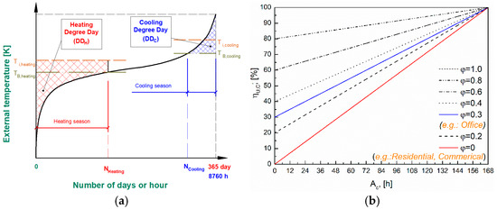
Figure 2.
Interpretation basis for (a) the degree days; (b) the utilisation efficiency for the buildings.
The following equation defines the balance point temperature [54]:
where ‘Ti’ is the internal temperature, in [K]. ‘’ is the solar heat gain, and ‘’ represents internal heat gains, both in [W]. ‘Htr’ is the transmission heat loss coefficient, in [W·K−1]. ‘c’ is the specific heat capacity of air, in [J·kg−1·K−1], ‘ρ’ is the air density in [kg·m−3], ‘V’ is the volume of the examined room, in [m3], and ‘n’ is the air exchange rate, in [h−1].
Equation (2) calculates the cooling degree-day value (DDC) [55]:
where ‘Te’ is the external temperature, in [K].
To estimate the energy demand of the building, it is advantageous to incorporate the weekly utilisation efficiency (ηU,C), which reflects the functional attributes of the building (Figure 2b) [55]:
where ‘AC’ is the number of active hours per week from a human usage perspective, in hours. ‘φ’ is the passivity operating ratio during inactive periods compared to active periods, [-].
These parameters determine the energy demand (EC) using the following expression [55]:
Although typically applied on an annual scale, these equations are also applicable to daily-scale analysis. In such cases, the temperature–frequency curve and the balance point–temperature curve exhibit greater segmentation due to the smaller number of available data points (e.g., hourly temperature records), which reduces numerical precision but remains suitable for comparative analyses and trends evaluation.
2.2. Conditions and Constraints for Equivalent Free Cooling Replacement
As previously established, free cooling occurs when the external temperature is lower than the desired indoor temperature. Section 2.1 defines the balance point temperature, which refines the condition for free cooling as TB < Te < Ti. To assess free cooling potential, the daily scale provides the most appropriate resolution. Accordingly, a representative day with suitable external conditions is selected. The hourly temperature values of this day are arranged to form a temperature–frequency curve, analogous to the annual curve introduced earlier, but applied at the daily resolution.
This curve also includes the design indoor temperature and the balance point temperature, both represented as guide linear segments. Equation (1) defines how the balance point temperature varies over the course of a day. In periods without solar radiation, the balance point temperature remains constant as a horizontal segment. However, in sunlit hours, it gradually decreases with minor fluctuations due to varying radiative gains. To maintain clarity, Figure 3 excludes these hourly fluctuations.
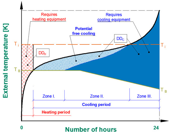
Figure 3.
Stylised temperature–frequency curve of a typical early summer day.
The driving factor of free cooling is the temperature difference between indoor and outdoor conditions. Figure 3 also displays the part of the DDC that represents potential free cooling on the (hourly) temperature–frequency curve. This zone consists of the area bounded by the balance point temperature line, the external temperature line, and an auxiliary curve. Subtracting the hourly temperature difference between indoor and outdoor air from the external temperature constructs this auxiliary curve. This auxiliary curve separates the DDC into three distinct zones at a selected air exchange rate. These zones reflect the varying feasibility of replacing mechanical cooling with free cooling. Zone I represents the range where mechanical cooling is completely replaceable by an equivalent free cooling solution, while Zone III excludes the possibility of such replacement. Zone II spans the intermediate range, where mechanical cooling is only partially replaceable by free cooling.
Industrial and comfort-sector users aim to minimise mechanical cooling demand. Based on Figure 3, two distinct strategies are identified to achieve this target. One strategy involves fully exploiting the potential of free cooling, a concept already reflected in the literature. The other focuses on reducing the Ti − TB temperature difference, as lower values directly reduce mechanical cooling demand. Adjusting Ti is generally impractical, as it directly affects thermal comfort [56] and is prescribed by design standards and legislation. Deviations from standard values are only considered when specific design requirements justify the adjustment. Therefore, Ti remains constant in the present analysis.
The alternative is to modify TB. According to Equation (1), TB increases with higher air exchange rates. If the air exchange rate approaches infinity, TB equals Ti, and mechanical cooling demand reaches its theoretical minimum. However, an upper technological limit and an economic threshold [25,30] constrain this approach. Regulations specify no values above 20 [h−1] [57,58]. This study adopts this value as the upper technological limit. However, the 20 [h−1] air exchange rate also serves as a threshold, as typical systems reach this value only by accepting oversized ductwork, excessive airflow volumes, or elevated noise levels. The economic threshold marks the point where the electricity demand of mechanical ventilation exceeds that of the cooling equipment. In other words, beyond this threshold, a free cooling system operates less cost-effectively than a mechanical cooling system. The air exchange rate at the economic threshold, denoted as nmax, is a central focus of this study. More precisely, the analysis examines the additional air change rate (∆n) that raises the minimum fresh air requirement defined by the building function (nmin) to nmax, thereby enhancing the significance of free cooling.
3. Results
The following analysis examines the impact of increasing the minimum air change rate (nmin) by ∆n on the avoided mechanical cooling energy (∆EC). In other words, the fresh air requirement defined by the building function is satisfied (nmin), and enhanced free cooling (EFC) operates beyond this minimum (nmin + ∆n).
The analysis builds on the concept of the economic threshold, as defined in Section 2.2, and incorporates practical aspects. These aspects include system inertia, control hysteresis, the alternation between mechanical and free cooling modes, or the advantages of a less complex technological implementation. A mechanical correction factor, denoted as ‘z’, represents their combined effect. Thus, the EFC is economically viable when the additional ventilation work (∆WVE) remains below the avoided electrical work of mechanical cooling (∆WCU) corrected by factor ‘z’:
where ‘z’ is the HVAC system correction factor, [-]. Furthermore ‘∆τVE’ is the operating period of EFC, in [s].
Equation (1) also reveals that the TB approaches Ti as the air change rate increases. Figure 3 indicates that this reduces the potential free cooling zone, thereby decreasing ∆τve.
In the next step, specific expressions replace the two work terms in Equation (5). The ∆WCU is the ratio of the ∆EC and the SCOPR. The ∆EC represents a saved energy; therefore, the sign is negative. As a result, Equation (6) applies the reversed direction of the inequality. The ∆WVE equals the product of the total pressure difference created by the fan (∆pt), the room volume (V), the ∆n, and the reciprocal of the fan efficiency (1/ηve):
where ‘SCOPR’ is the Seasonal Coefficient of Performance of the cooling unit, [-]; ‘∆pt’ is the total pressure increase created by the fan, in [Pa]; ‘ηve’ is the overall efficiency of the fan, [-].
The rearrangement of Equation (6) determines ∆EC, and also reveals its upper limit (∆EC,max):
Equation (7) indicates that the ∆EC,max depends on mechanical (SCOPR, ∆pt, ηve), geometrical (V), and operational (z, ∆τve, ∆n) parameters. Dividing ∆EC by ∆EC,max defines the efficiency of enhanced free cooling:
The precise determination of this efficiency is difficult because operational parameters have complex interdependencies. However, a case study provides a practical framework for further analysis. Before proceeding, the development process of the analytical model is briefly summarised (Figure 4).
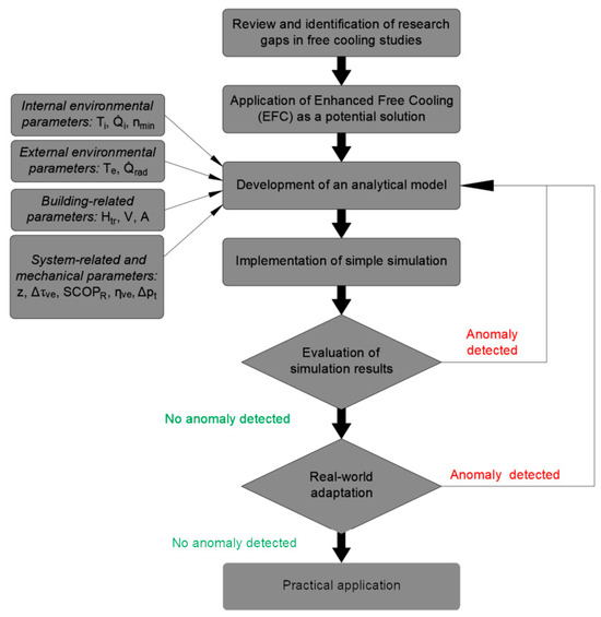
Figure 4.
Logical structure of the analytical modelling development.
The subsequent case study corresponds to a “simple simulation implementation”.
4. Case Study and Discussion
4.1. The Analysed Room and the Changed Parameter
The case study considers a room (Figure 5) located on the third floor of a four-story building. This room has two external walls (Uwall = 0.24 W∙m−2∙K−1) with partial glazing (Uglass = 1.1 W∙m−2∙K−1). These thermal transmittance values comply with the requirements of the Hungarian ÉKM Decree 9/2023 [57]. The floor area is 61.45 m2, and the air volume is 174.35 m3. Due to a partially suspended ceiling, the ceiling height varies, measuring 3 m near the glazed surface and 2.5 m near the door. Figure 5 highlights the area below the suspended ceiling in green. The transmission heat loss coefficient of the room envelope (HTR) is 16.49 W∙K−1.
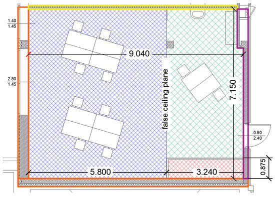
Figure 5.
The design of the analysed room. Orange—External wall, Yellow—Internal wall facing the room, Purple—Internal wall facing the corridor, Blue—Ceiling height of 3 m, Green—Ceiling height of 2.5 m, Red—Built-in area.
The numerical analysis applies Microsoft Excel LTSC Professional Plus 2021, provided under a university licence. The design of simple simulation scenarios considers that the glazing ratio and orientation significantly influence the Qrad value and, consequently, the cooling energy demand (based on Equations (1)–(4)). The outdoor environment is also represented by the external temperature, which justifies the inclusion of individual meteorological days in the analysis. Furthermore, the internal conditions are represented by two operational categories (buildings with continuous use, such as residential units, and buildings with intermittent occupancy, such as office and small commercial facilities). Therefore, this analysis addresses three functional categories: commercial (e.g., retail space), office, and residential (e.g., living room), which are commonly represented in the Hungarian building stock [59]. Figure 5 illustrates the interior layout of the office function, while Table 1 summarises the parameters varied in the analysis.

Table 1.
Parameters varied in the analysis.
According to ISO 7730 [60], the Ti is 24.5 °C. Three meteorological day types (summer, hot, and extremely hot days (Summer/Hot/Extremely Hot Day: On a given day, the hourly average temperature is at least 25 °C, 30 °C, or 35 °C, respectively [4])) characterise periods relevant for free cooling. Selection relies on the Debrecen meteorological dataset from the period 2009 to 2019. For each year, the classification categorises all meteorological days into the three target types. Within each year, the procedure identifies the day with the maximum daily temperature fluctuation for each category. The selection process assigns, for each category, the year with the minimum daily temperature fluctuation in the final step. The second step selects days with high energy-saving potential, while the third excludes days with rapid weather changes (e.g., sunny morning followed by a rainy afternoon). Figure 6 demonstrates the selected days.
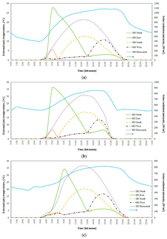
Figure 6.
The selected target days: (a) the summer day: 9 August 2016; (b) the hot day: 15 August 2010; (c) the extremely hot day: 4 August 2017.
Internal heat gains (from occupants, equipment, etc.) are defined according to EN ISO 13790 [61]. Energy demand calculations include the air exchange rate (nmin) assigned to each functional category. This rate is determined based on the number of occupants and the fresh air requirement per person. For mechanical ventilation and cooling systems, the applied mechanical parameters follow the recommendations of ÉKM Decree 9/2023 [57]. Table 2 summarises these values.
Table 2.
Data considered for HVAC systems.
A glazing ratio of 40% is applied based on Goia’s results [62], which identified this value as representative for typical building applications.
4.2. Savings Analysis with the Application of Enhanced Free Cooling
The following analysis applies Equation (7) to quantify the avoided mechanical cooling energy (∆EC) via enhanced free cooling (EFC). For this calculation, the HVAC system correction factor (z) requires an exact value. Determinant of the value of z involves expert input from HVAC system designers. According to professional consensus, accurate estimation requires detailed system design. Accurate value requires consideration of multiple factors, including the building function, the response time of the HVAC system (fast or slow), and the degree of system separability (lower z values for well-separated systems, higher z values for complex systems with limited modulation). These factors are interdependent and scenario-dependent. After consultation with HVAC system designers, a fixed increment of 10% is applied (z = 1.1) in this article. The applied value reflects standard engineering practice in Hungary, as validated by consultation with practising HVAC designers. Applicability in international contexts appears likely; however, precise adjustment requires coordination with local HVAC professionals.
The first analysis examines ∆EC (as a proportion of the original mechanical cooling demand, EC) across different glazing ratios and orientations (EFC applied). Figure 7 presents the results (case notations as defined in Table 4):
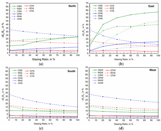
Figure 7.
Change in mechanical cooling energy savings with varying glazing ratios. (a) North orientation, (b) east orientation, (c) south orientation, and (d) west orientation.
Result interpretation considers a 10% cooling energy saving as a reasonable minimum threshold for a 10% increase in electrical work (z = 1.1). North orientation (Figure 7a) achieves this threshold for the residential building on all target days and for the office building on the summer day, while the commercial building remains below this level. East orientation (Figure 7b) adds further threshold achievements, including the office building on the hot day and the commercial building on the summer day. South orientation (Figure 7c) meets the threshold for the residential building on both the hot and extremely hot days, with the office and residential buildings approaching this level on the summer day. West orientation (Figure 7d) again results in a distinct pattern, where the residential building reaches the threshold, and the office building on the summer day remains slightly below this level.
The highest cooling energy savings occur with an east orientation and high glazing ratios (above 60%) as observed on a summer day. Values range from 37.62% to 40.12% for the residential building, 49.63% to 57.81% for the office, and 26.45% to 45.22% for the commercial facility, depending on the type of glazing. The lowest savings occur with south orientation and high glazing ratios. The residential building reaches 7.59–8.54% on the summer day. However, values reach 0.85–0.80% for the commercial facility and 2.01–1.62% for the office, on a hot day. Greater glazing ratios correspond to more pronounced variability, as both maximum and minimum values relate to high glazing.
Before drawing further conclusions, Table 3 presents the mechanical cooling energy savings at a fixed glazing ratio (40%). For clarity, in comparison with Figure 7, the table expresses the values as percentages.
Table 3.
Mechanical cooling energy savings with a 40% glazing ratio and z = 1.1 (EFC applied).
Table 3 and Figure 7 indicate that east orientation supports EFC more effectively, while south orientation provides minimal advantage. The highest cooling energy savings occur in the residential building, among the examined building types. Increasing daily maximum external temperature generally reduces savings. However, within the residential building type, this effect remains least pronounced. In several cases (particularly with north, south, and west orientations), higher temperatures correspond to increased savings. The analysis results corroborate initial hypotheses based on informal case reviews, suggesting broader applicability of the observed trends to comparable cases. However, these results derive from a single building model; therefore, generalisation requires caution. EFC achieves the highest savings when the temperature difference between indoor and outdoor air peaks, typically in the early morning. At this time, east-facing orientations receive the strongest solar gains, which reduce the required TB value (Equation (1)), increase DDC (Equation (2)), and raise cooling demand (Equation (4)). EFC offsets this increment effectively, resulting in greater relative energy savings.
The following section evaluates the variation in the efficiency of enhanced free cooling (ηfc) across different orientations, target days, and glazing ratios. Figure 8 presents these results (case notations as in Figure 7, defined in Table 4).
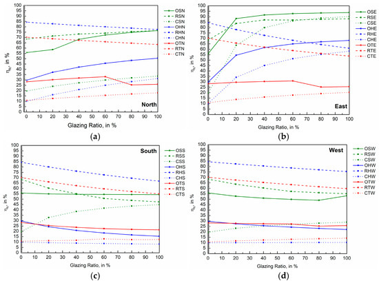
Figure 8.
The variation in the efficiency of enhanced free cooling (ηfc): (a) north orientation; (b) east orientation; (c) south orientation; (d) west orientation.
Table 4.
The nmax values at z = 1.1, in h−1.
Based on Figure 8, the ηfc values indicate significant variability. This variability warrants a detailed examination of ηfc by orientation, target day, and building type, evaluated as a function of glazing ratio. Generally, higher glazing ratios reduce ηfc variability, regardless of building function. The residential building exhibits the highest fluctuation (74.11%), independent of each orientation. By contrast, the office building exhibits the lowest fluctuation, with values depending on orientation (north: 42.87% in Figure 8a; east: 5.72% in Figure 8b; south: 9.27% in Figure 8c; and west: 26.14% in Figure 8d).
In HVAC system design, minimising efficiency fluctuation represents a general design objective. Stable ηfc values improve the predictability of cooling energy demand, which supports accurate equipment sizing and control calibration. Near constant ηfc value simplifies commissioning, verification, and long-term assessment. In EFC control, reduced fluctuation enables demand-driven operation and also supports the applicability of robust automation strategies. This overall effect supports reliable and cost-efficient HVAC system design. From this perspective, east-facing buildings with high glazing ratios offer the most stable ηfc values. The results also emphasise the need to account for building orientation and glazing ratio in HVAC system design, particularly when applying EFC.
4.3. Air Exchange Rate Thresholds and EFC Resistance Points
This section evaluates the available range of operational air exchange rates and their impact on mechanical cooling energy savings. As previously defined, nmin represents the minimum fresh air requirement based on building function, while nmax denotes the economic threshold (applied at z = 1.1) beyond which enhanced free cooling (EFC) becomes less cost-effective. The values of nmax, as presented in Table 4, vary with orientation, glazing ratio, and external temperature. Values exceeding the previously established technological limit of 20 [h−1] are highlighted in red, as such rates are likely to encounter feasibility constraints. This limit reflects current regulatory principles, as noted earlier.
In most cases, increasing the glazing ratio enhances the available range of air exchange rates. However, several cases (Table 4: OSE, OTN, OTE, OTS, OTW) exhibit a non-monotonic trend. In these cases, nmax initially increases with glazing ratio up to a certain threshold, then undergoes a sharp decline before resuming steady growth at higher glazing ratios. This behaviour suggests the existence of an optimal glazing ratio that maximises the achievable air exchange rate range for a given technological limit (e.g., 20 h−1). This aspect lies beyond the scope of the present study, and future research investigates it as a defined objective.
In the remainder of the analysis, calculations apply the upper limit of 20 [h−1] wherever the value of nmax exceeds it. The range defined by nmin and nmax varies considerably. Hence, for comparative clarity, the evaluation considers only values corresponding to a 40% glazing ratio. Figure 9 illustrates the results for each functional category.
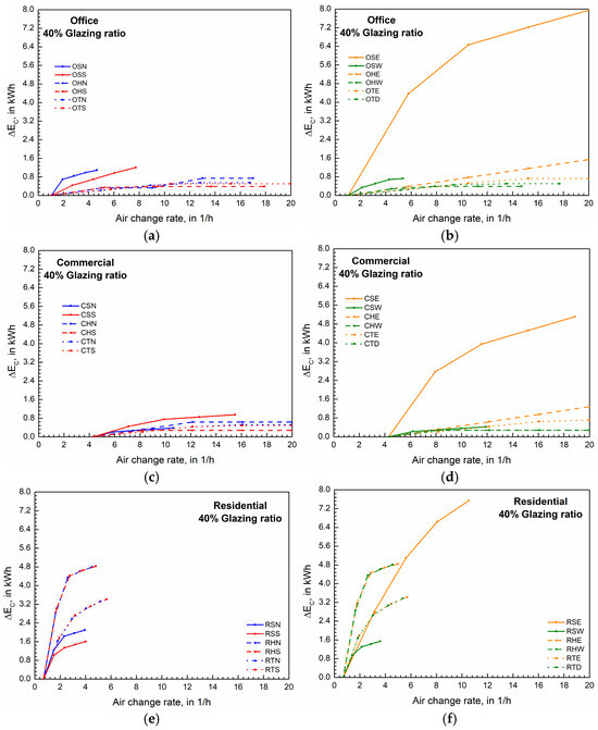
Figure 9.
Mechanical cooling energy savings as a function of air exchange rate between nmin and nmax; (a,b) office building; (c,d) commercial building; (e,f) residential building.
The available range of air exchange rate adjustment is highest in the office function type, followed by the commercial, and lowest in the residential building function. Within each functional category, east-facing orientations allow the broadest range of air exchange rate adjustment. The effect of orientation is the largest on the summer target day, and becomes weaker on the hot day, and is the least on the extremely hot day. In several cases of the office and the commercial building types, increasing the air exchange rate fails to reduce cooling energy demand. The values of these cases are examined separately and complemented by their corresponding ηfc values. Figure 10 displays the results.
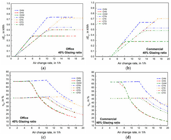
Figure 10.
Determination of the nopt value. (a) Office building: cooling energy savings as a function of air exchange rate; (b) commercial building: cooling energy savings as a function of air exchange rate; (c) office building: ηfc as a function of air exchange rate; (d) commercial building: ηfc as a function of air exchange rate.
Figure 10 identifies cases where increasing the air exchange rate fails to improve mechanical cooling energy savings. This threshold defines the resistance point of EFC, where the corresponding air exchange rate represents the optimal value (nopt). This resistance point corresponds to the point of diminishing savings, as well. Beyond this, further increases in air exchange rate result in negligible cooling energy savings while continuously increasing fan electricity demand. As shown in Figure 10c,d, ηfc reaches its maximum at this point and subsequently decreases. Table 5 demonstrates the nopt values and their impact on cooling energy savings for the separated cases, at a glazing ratio of 40%.
Table 5.
Achievable mechanical cooling energy savings and ηfc values at nopt.
In the 14 examined cases, selecting nopt (nopt < nmax) as the operational air exchange rate in the EFC system maintains the maximum cooling energy savings (ΔEC). Table 5 lists the 14 separated cases in decreasing order of the nopt/nmax ratio. A lower value corresponds to a greater reduction in fan electricity demand in EFC operation. The maximum difference appears in case OHS (nopt/nmax = 0.3233), while the minimum occurs in case CTE (nopt/nmax = 0.8560). Table 5 lists hot-day cases first, followed by extremely-hot-day cases. On the hot day, the nopt/nmax ratio remains lower (0.3233–0.3936) than on the extremely hot day (0.5090–0.8560). On the hot day, this results in a greater potential reduction in fan electricity demand in EFC operation.
The resistance analysis extends to the remaining cases. Preliminary results indicate a more complex connection between nopt and the extreme values of ηfc. Clarification of these connections requires additional target days, and the next phase of the research addresses this need.
5. Conclusions
Significant reduction in mechanical cooling energy demand is the focus of this article. The efficient exploitation of free cooling potential supports this objective. One applicable method is enhanced free cooling (EFC), which increases the air exchange rate to free cooling. The manuscript demonstrates the practical potential of EFC across multiple building functions and orientations. The introduced metric, the efficiency of enhanced free cooling (ηfc), quantifies how effectively EFC exploits available outdoor cooling potential for the reduction in mechanical cooling energy demand (that is, for increasing the avoided mechanical cooling energy, ΔEC). The findings offer operational guidance for retrofits and low-cost control strategies that reduce mechanical cooling demand while maintaining occupant comfort. The case study developed for this purpose provides quantifiable data for evaluating the EFC applied.
Demonstrated results confirm that the highest specific mechanical cooling energy savings (49.63%) occur in the east-facing office building with a 40% glazing ratio on the summer day. For the residential building, savings are lower on this summer day (37.78%) but remain more stable on the hot and extremely hot days (19.54% and 12.86%, respectively) compared to the office building (12.71% and 3.81%). The impact of building orientation diminishes with increasing external temperature. Additionally, increasing the glazing ratio stabilises the ηfc value across the examined temperature conditions. The analysis of air exchange rate and mechanical cooling energy savings identifies the resistance point of free cooling in 14 cases. This point defines the optimal air exchange rate (nopt), beyond which further increases result in no additional mechanical cooling energy savings. In all 14 cases, ηfc reaches its maximum at nopt. Determining nopt is therefore essential for efficient utilisation of free cooling potential. However, generalisation requires further investigation, as the results are specific to the parameters of the present case study. These additional investigations include measurements performed under real operating conditions and in controlled laboratory environments. Both measurement types are in progress, with initial findings indicating promise.
Gradual extension of the present results offers several directions for further research, each of which represents a potential study. One avenue is the seasonal analysis extended across the complete cooling season. Another lies in the detailed investigation of HVAC systems that integrate the free and the mechanical cooling. Further opportunities include the inclusion of alternative cooling technologies, such as absorption chillers, as well as the systematic evaluation of the interaction between air exchange rates and glazing ratios. The relationship between nopt and the extreme values of ηfc also merits closer examination. Advancing along these lines supports the optimisation of free cooling strategies across diverse building types and contributes to sustainable building operation and HVAC design development.
Author Contributions
Conceptualization: G.L.S.; Methodology: G.L.S. and E.B.; Software: E.B. and S.J.; Validation: E.B. and S.J.; Formal analysis: G.L.S., E.B. and S.J.; Investigation: G.L.S., E.B. and S.J.; Resources: G.L.S. and E.B.; Data Curation: G.L.S.; Writing—Original Draft: G.L.S.; Writing—Review and Editing: G.L.S. and E.B.; Visualization: G.L.S. and E.B.; Supervision: G.L.S.; Project administration: G.L.S.; Funding acquisition: G.L.S. All authors have read and agreed to the published version of the manuscript.
Funding
Project no. TKP2021-NKTA-34 has been implemented with the support provided from the National Research, Development and Innovation Fund of Hungary, financed under the TKP2021-NKTA funding scheme.
Data Availability Statement
The data presented in this study are available on request from the corresponding author.
Acknowledgments
The authors would like to express their gratitude for Agro-Meteorological Observatory Debrecen for providing indispensable meteorological data.
Conflicts of Interest
The authors declare no conflicts of interest. The funders had no role in the design of the study; in the collection, analyses, or interpretation of data; in the writing of the manuscript; or in the decision to publish the results.
Nomenclature
| ‘TB’ | is the balance point temperature, in [K]. |
| ‘’ | is the solar heat gains, in [W]. |
| ‘’ | is the internal heat gains, in [W]. |
| ‘Ti’ | is the internal temperature, in [K]. |
| ‘Te’ | is the environmental temperature, in [K]. |
| ‘Htr’ | is the transmission heat loss coefficient [W∙K−1]. |
| ‘c’ | is the specific heat capacity of air, in [J·kg−1 ·K−1]. |
| ‘ρ’ | is the air density, in [kg·m−3]. |
| ‘n’ | is the air change rate, in [h−1]. |
| ‘V’ | is the volume of the examined room, in [m3]. |
| ‘DDC’ | is the cooling degree-day value, in [h·K]. |
| ‘DDH’ | is heating degree-day value, in [h·K]. |
| ‘Te’ | is the external temperature, in [K]. |
| ‘ηU,C’ | is the weekly utilisation efficiency for the building (cooling mode), in [%]. |
| ‘AC’ | is the number of active hours per week from a human usage perspective, in [h]. |
| ‘φ’ | is the passivity operating ratio during inactive periods compared to active periods, in [-]. |
| ‘EC’ | is the cooling energy demand, in [Wh]. |
| ‘nmin’ | is the air change rate based on the human fresh air requirement, in [h−1]. |
| ‘nmax’ | is the air change rate at the economic threshold and z = 1.1, in [h−1]. |
| ‘Δn’ | is the additional air change rate required to reach nmax, in [h−1] |
| ‘ΔEC’ | is the avoided mechanical cooling energy demand, in [kWh]. |
| ‘ECmax’ | is the avoided mechanical cooling energy demand upper limit, in [Wh]. |
| ‘z’ | is the HVAC system correction factor, in [-]. |
| ‘ΔWVE’ | is the additional ventilation electric work, in [kWh]. |
| ‘ΔWCU’ | is the avoided electrical work of mechanical cooling, in [kWh]. |
| ‘Δτve’ | is the operating period of EFC, in [s] |
| ‘SCOPR’ | is the Seasonal Coefficient of Performance of the cooling unit, in [-]. |
| ‘∆pt’ | is the total pressure increase created by the fan, in [Pa] |
| ‘ηve’ | is the overall efficiency of the fan, in [-]. |
| ‘ηfc’ | is the efficiency of enhanced free cooling, in [%] |
| ‘nopt’ | is the optimal air change rate, in [h−1]. |
References
- The European Parliament and the Council of the European Union. Directive 2010/30/EU of the European Parliament and of the Council; on the indication by labelling and standard product information of the consumption of energy and other resources by energy-related products (recast). Off. J. Eur. Union 2010, 153, 1–12. Available online: http://eur-lex.europa.eu/legal-content/EN/TXT/PDF/?uri=CELEX:32010L0030&from=EN (accessed on 20 August 2025).
- Kalmár, F.; Kalmár, T. Reduction of Energy Use for Heating in Detached Housés using Passive Technics. Int. J. Eng. Manag. Sci. 2022, 7, 64–76. [Google Scholar] [CrossRef]
- Szodrai, F.; Lakatos, Á.; Kalmár, F. Analysis of the change of the specific heat loss coefficient of buildings resulted by the variation of the geometry and the moisture load. Energy 2016, 115, 820–829. [Google Scholar] [CrossRef]
- Kostyák, A.; Szekeres, S.; Csáky, I. Assessment of the Actual and Required Cooling Demand for Buildings with Extensive Transparent Surfaces. Energies 2024, 17, 5814. [Google Scholar] [CrossRef]
- Kalmár, F.; Bodó, B.; Li, B.; Kalmár, T. Decarbonization Potential of Energy Used in Detached Houses—Case Study. Buildings 2024, 14, 1824. [Google Scholar] [CrossRef]
- Kalmár, F. Interrelation between glazing and summer operative temperature in buildings. Int. Rev. Appl. Sci. Eng. IRASE 2016, 7, 51–60. [Google Scholar] [CrossRef]
- Csáky, I.; Kalmár, T. Analysis of degree day and cooling energy demand in educational buildings. Environ. Eng. Manag. J. 2014, 13, 2765–2770. [Google Scholar] [CrossRef]
- Csáky, I. Analysis of daily energy demand for cooling in buildings with different comfort categories—Case study. Energies 2021, 14, 4694. [Google Scholar] [CrossRef]
- Santamouris, M. Cooling the buildings—Past, present and future. Energy Build. 2016, 128, 617–638. [Google Scholar] [CrossRef]
- Li, X.; Wu, W.; Yu, C.W.F. Energy demand for hot water supply for indoor environments: Problems and perspectives. Indoor Built Environ. 2015, 24, 5–10. [Google Scholar] [CrossRef]
- Akinyemi, T.; Jung, S. Power plants improve local residents’ wealth: A case study of Nigeria. Energy Econ. 2025, 142, 108131. [Google Scholar] [CrossRef]
- Prataviera, E.; Zarrella, A.; Morejohn, J.; Narayanan, V. Exploiting district cooling network and urban building energy modeling for large-scale integrated energy conservation analyses. Appl. Energy 2024, 356, 122368. [Google Scholar] [CrossRef]
- Neri, M.; Guelpa, E.; Khor, J.O.; Romagnoli, A.; Verda, V. Hierarchical model for design and operation optimization of district cooling networks. Appl. Energy 2024, 371, 123667. [Google Scholar] [CrossRef]
- Szabó, G.L. Energetic and exergetic study of a potential interconnection of a natural gas engine, heat pumps with a thermal and a mechanical compressor. Therm. Sci. Eng. Prog. 2022, 36, 101525. [Google Scholar] [CrossRef]
- Chen, Y.; Zhang, X. Research progress of energy-saving technology in cold storage with/without phase change materials. J. Energy Storage 2024, 103, 114334. [Google Scholar] [CrossRef]
- Guo, Z.; Qiao, J.; Liu, X.; Lin, F.; Liu, M.; Fang, M.; Huang, Z.; Zhang, X.; Min, X. Advances in mineral-based composite phase change materials for energy storage: A review. Green Smart Min. Eng. 2024, 1, 447–473. [Google Scholar] [CrossRef]
- Lakatos, Á.; Kalmár, F.; Csáky, I. Material selection in order to minimize the heat loss of piping based on measurements and calculations. AIP Conf. Proc. 2019, 2186, 070011. [Google Scholar] [CrossRef]
- Kostyák, A.; Béres, C.; Szekeres, S.; Csáky, I. Buffer Tank Discharge Strategies in the Case of a Centrifugal Water Chiller. Energies 2023, 16, 188. [Google Scholar] [CrossRef]
- Vassiliades, C.; Barone, G.; Buonomano, A.; Forzano, C.; Giuzio, G.F.; Palombo, A. Assessment of an innovative plug and play PV/T system integrated in a prefabricated house unit: Active and passive behaviour and life cycle cost analysis. Renew. Energy 2022, 186, 845–863. [Google Scholar] [CrossRef]
- Szkordilisz, F.; Kiss, M. Passive cooling potential of alley trees and their impact on indoor comfort. Pollack Period. 2016, 11, 101–112. [Google Scholar] [CrossRef][Green Version]
- Dehwah, A.H.A.; Krarti, M. Energy performance of integrated adaptive envelope systems for residential buildings. Energy 2021, 233, 121165. [Google Scholar] [CrossRef]
- Güğül, G.N.; Gökçül, F.; Eicker, U. Sustainability analysis of zero energy consumption data centers with free cooling, waste heat reuse and renewable energy systems: A feasibility study. Energy 2023, 262, 125495. [Google Scholar] [CrossRef]
- Do, H.; Cetin, K.S. Mixed-Mode Ventilation in HVAC System for Energy and Economic Benefits in Residential Buildings. Energies 2022, 15, 4429. [Google Scholar] [CrossRef]
- Wenzel, P.M.; Mühlen, M.; Radgen, P. Free Cooling for Saving Energy: Technical Market Analysis of Dry, Wet, and Hybrid Cooling Based on Manufacturer Data. Energies 2023, 16, 3661. [Google Scholar] [CrossRef]
- Aili, A.; Long, W.; Cao, Z.; Wen, Y. Radiative free cooling for energy and water saving in data centers. Appl. Energy 2024, 359, 122672. [Google Scholar] [CrossRef]
- Yang, Y.; Wang, B.; Zhou, Q. Air Conditioning System Design using Free Cooling Technology and Running Mode of a Data Center in Jinan. Procedia Eng. 2017, 205, 3545–3549. [Google Scholar] [CrossRef]
- Zhang, H.; Shao, S.; Xu, H.; Zou, H.; Tian, C. Free cooling of data centers: A review. Renew. Sustain. Energy Rev. 2014, 35, 171–182. [Google Scholar] [CrossRef]
- Li, J.; Li, Z. Model-based optimization of free cooling switchover temperature and cooling tower approach temperature for data center cooling system with water-side economizer. Energy Build. 2020, 227, 110407. [Google Scholar] [CrossRef]
- van Moeseke, G.; Bruyère, I.; De Herde, A. Impact of control rules on the efficiency of shading devices and free cooling for office buildings. Build. Environ. 2007, 42, 784–793. [Google Scholar] [CrossRef]
- Xu, T.; Jing, Y.; Madani, H.; Xie, X.; Jiang, Y. Applying indirect evaporative chillers for comfort cooling in Northern European commercial buildings: A case study in Sweden. Appl. Therm. Eng. 2024, 248, 123158. [Google Scholar] [CrossRef]
- Amado, E.A.; Schneider, P.S.; Bresolin, C.S. Free cooling potential for Brazilian data centers based on approach point methodology. Int. J. Refrig. 2021, 122, 171–180. [Google Scholar] [CrossRef]
- Cho, J.; Lim, T.; Kim, B.S. Viability of datacenter cooling systems for energy efficiency in temperate or subtropical regions: Case study. Energy Build. 2012, 55, 189–197. [Google Scholar] [CrossRef]
- Kwon, T.D.; Jeong, J.W. Energy advantage of cold energy recovery system using water- and air-side free cooling technologies in semiconductor fabrication plant in summer. J. Build. Eng. 2023, 69, 106277. [Google Scholar] [CrossRef]
- Mi, R.; Bai, X.; Xu, X.; Ren, F. Energy performance evaluation in a data center with water-side free cooling. Energy Build. 2023, 295, 113278. [Google Scholar] [CrossRef]
- Cai, S.; Gou, Z. Towards energy-efficient data centers: A comprehensive review of passive and active cooling strategies. Energy Built Environ. 2024; in press. [Google Scholar] [CrossRef]
- Desideri, U.; Sorbi, N.; Arcioni, L.; Leonardi, D. Feasibility study and numerical simulation of a ground source heat pump plant, applied to a residential building. Appl. Therm. Eng. 2011, 31, 3500–3511. [Google Scholar] [CrossRef]
- Lee, K.P.; Chen, H.L. Analysis of energy saving potential of air-side free cooling for data centers in worldwide climate zones. Energy Build. 2013, 64, 103–112. [Google Scholar] [CrossRef]
- Zhao, W.; Li, H.; Wang, S. A generic design optimization framework for semiconductor cleanroom air-conditioning systems integrating heat recovery and free cooling for enhanced energy performance. Energy 2024, 286, 129600. [Google Scholar] [CrossRef]
- Ljungqvist, H.M.; Risberg, M.; Toffolo, A.; Vesterlund, M. A realistic view on heat reuse from direct free air-cooled data centres. Energy Convers. Manag. X 2023, 20, 100473. [Google Scholar] [CrossRef]
- Hnayno, M.; Chehade, A.; Klaba, H.; Polidori, G.; Maalouf, C. Experimental investigation of an optimized indirect free cooling system including a dry cooler equipped with evaporative cooling pads for data center. Energy Rep. 2023, 9, 460–469. [Google Scholar] [CrossRef]
- Depoorter, V.; Oró, E.; Salom, J. The location as an energy efficiency and renewable energy supply measure for data centres in Europe. Appl. Energy 2015, 140, 338–349. [Google Scholar] [CrossRef]
- Ham, S.W.; Park, J.S.; Jeong, J.W. Optimum supply air temperature ranges of various air-side economizers in a modular data center. Appl. Therm. Eng. 2015, 77, 163–179. [Google Scholar] [CrossRef]
- Ham, S.W.; Kim, M.H.; Choi, B.N.; Jeong, J.W. Energy saving potential of various air-side economizers in a modular data center. Appl. Energy 2015, 138, 258–275. [Google Scholar] [CrossRef]
- Hellmer, B.A. Consumption Analysis of Telco and Data Center Cooling and Humidification Options. ASHRAE Trans. 2010, 116, 118–133. [Google Scholar]
- Lamptey, N.B.; Anka, S.K.; Lee, K.H.; Cho, Y.; Choi, J.W.; Choi, J.M. Comparative energy analysis of cooling energy performance between conventional and hybrid air source internet data center cooling system. Energy Build. 2024, 302, 113759. [Google Scholar] [CrossRef]
- Lubis, A.; Giannetti, N.; Alhamid, M.I.; Saito, K.; Yabase, H. Dynamic analysis of single–double-effect ab-sorption chiller with variable thermal conductance during partial-load operation. Appl. Therm. Eng. 2023, 218, 119424. [Google Scholar] [CrossRef]
- Rabczak, S.; Nowak, K. Possibilities of Adapting a Free-Cooling System in an Existing Commercial Building. Energies 2022, 15, 3350. [Google Scholar] [CrossRef]
- Jayasekara, S.; Halgamuge, S.K. Mathematical modeling and experimental verification of an absorption chiller including three dimensional temperature and concentration distributions. Appl. Energy 2013, 106, 232–242. [Google Scholar] [CrossRef]
- Boukholda, I.; Ben Ezzine, N.; Bellagi, A. Experimental investigation and simulation of commercial absorption chiller using natural refrigerant R717 and powered by Fresnel solar collector. Int. J. Thermofluids 2025, 27, 101213. [Google Scholar] [CrossRef]
- Kailkhura, G.; Mandel, R.K.; Shooshtari, A.; Ohadi, M. A 1D Reduced-Order Model (ROM) for a Novel Latent Thermal Energy Storage System. Energies 2022, 15, 5124. [Google Scholar] [CrossRef]
- Evola, G.; Costanzo, V.; Marletta, L. Exergy analysis of energy systems in buildings. Buildings 2018, 8, 180. [Google Scholar] [CrossRef]
- Dikmen, M.; Burns, C. The effects of domain knowledge on trust in explainable AI and task performance: A case of peer-to-peer lending. Int. J. Hum. Comput. Stud. 2022, 162, 102792. [Google Scholar] [CrossRef]
- Kim, Y.J.; Kim, K.H.; Ha, J.W.; Song, Y.H. Research on a Plan of Free Cooling Operation Control for the Efficiency Improvement of a Water-Side Economizer. Energies 2024, 17, 2804. [Google Scholar] [CrossRef]
- Verbai, Z.; Csáky, I.; Kalmár, F. Balance point temperature for heating as a function of glazing orientation and room time constant. Energy Build. 2017, 135, 1–9. [Google Scholar] [CrossRef]
- Bodó, B.; Béni, E.; Szabó, G.L. A Facility’s Energy Demand Analysis for Different Building Functions. Buildings 2023, 13, 1905. [Google Scholar] [CrossRef]
- Szabó, G.L.; Kalmár, F. Investigation of subjective and objective thermal comfort in the case of ceiling and wall cooling systems. Int. Rev. Appl. Sci. Eng. 2017, 8, 153–162. [Google Scholar] [CrossRef]
- Hungarian Ministry of Construction and Transport. Decree No. 9/2023 (V. 25.) of the Minister of Construction and Transport on the determination of the energy performance of buildings. Magy. Közlöny 2023, 78, 3462–3492. [Google Scholar]
- Hungarian Government. Government Decree No. 176/2008 (VI. 30.) on the certification of the energy performance of buildings. Magy. Közlöny 2008, 96, 5908–5915. [Google Scholar]
- Bodó, B.; Kalmár, F. Analysis of primary energy use of typical buildings in Hungary. Environ. Eng. Manag. J. 2014, 13, 2725–2731. [Google Scholar] [CrossRef]
- ISO 7730-1994; Moderate Thermal Environments-Determination of the PMV and PPD Indices and Specification of the Conditions for Thermal Comfort. International Organization for Standardization: Geneva, Switzerland, 1994.
- EN ISO 13790:2008; Energy Performance of Buildings—Calculation of Energy Use for Space Heating and Cooling. European Committee for Standardization: Brussels, Belgium, 2008.
- Goia, F. Search for the optimal window-to-wall ratio in office buildings in different European climates and the implications on total energy saving potential. Sol. Energy 2016, 132, 467–492. [Google Scholar] [CrossRef]


Disclaimer/Publisher’s Note: The statements, opinions and data contained in all publications are solely those of the individual author(s) and contributor(s) and not of MDPI and/or the editor(s). MDPI and/or the editor(s) disclaim responsibility for any injury to people or property resulting from any ideas, methods, instructions or products referred to in the content. |
© 2025 by the authors. Licensee MDPI, Basel, Switzerland. This article is an open access article distributed under the terms and conditions of the Creative Commons Attribution (CC BY) license (https://creativecommons.org/licenses/by/4.0/).