A Design-Oriented Unified Equation for the Torsion Constant of Non-Prismatic (Linearly Tapered) Rectangular Beams

Abstract

This study presents a unified, design-oriented equation for the torsion constant J of linearly tapered, non-prismatic rectangular members, covering two canonical geometries: (i) singly tapered bars, in which only the depth varies linearly along the longitudinal axis, and (ii) doubly tapered bars, in which both width and depth vary linearly. The formulation provides the spatial variation J(x) and enables evaluation of the associated shear stress distribution and angle of twist. Accuracy is assessed against classical elasticity solutions—Prandtl’s membrane analogy, single- and double-Fourier series solutions—as well as independent finite element analyses, demonstrating close agreement over a broad parametric range. A dimensionless coefficient $\varnothing (x)=J(x)/(b_2^3{h}_2)$ is introduced to elucidate trends: $\varnothing$ approaches 1/3 in the prismatic, very-narrow limit $({\lambda }_h={\lambda }_b=1,\alpha \approx 0)$, consistent with the exact solution; $\varnothing$ increases with increasing taper ratios in depth and width (${\lambda }_h,{\lambda }_b$) and decreases with increasing cross-sectional aspect ratio α. The proposed equation consolidates the treatment of tapered rectangular members into a single, practical framework, offering a computationally efficient tool for preliminary sizing and detailed design verification.

1. Introduction

For many years, torsion effects were regarded as secondary and were not considered explicitly in design; their influence was accounted for implicitly through factors of safety and conservative detailing. In modern practice, however, torsion is treated as a primary action, and dedicated design checks are performed for torsion in addition to those for shear and bending.

There are two types of torsion. The first—primary (equilibrium) torsion, also called statically determinate torsion—occurs when the external load has no alternative path and must be carried in torsion. The second—secondary (compatibility) torsion, or statically indeterminate torsion—arises from the requirements of continuity and deformation compatibility between adjacent structural members [1,2,3,4,5,6].

Most references address the torsion problem for circular cross sections, and the torsion of an elastic bar is commonly presented with results stated but without full proofs [7].

Saint-Venant’s theory of uniform torsion provides an exact solution for prismatic bars subjected to a constant torque. In this case, the warping displacement varies over the cross section but remains constant along the bar’s length. When an end is restrained against warping, the torque is no longer uniform along the member, and Saint-Venant’s uniform torsion theory cannot be applied directly; a warping (non-uniform) torsion formulation is required [8].

Beam theory with a single warping function is employed to study the behavior of thin-walled beams [9]. Results from finite element analyses and numerical examples are compared with established solutions to verify the proposed approach.

Tso and Ghobarah [10] investigated the nonlinear response of thin-walled, open-section elastic beams subjected to non-uniform torsion. They derived the governing differential equations and solved them using a perturbation method to obtain the torque–rotation relationship and the axial strain distribution. The solution’s accuracy and validity were verified through comparisons with experimental data and independent numerical results.

Campanile et al. [8] proposed a new theory for non-uniform torsion in beams with axisymmetric cross sections. The formulation employs a Fourier-series representation of the warping displacement and the unit-twist functions. Two benchmark examples—one open-section beam and one closed-section beam—are presented, and the predictions show very good agreement with classical solutions.

Louis et al. [11] presented an approximate solution to the torsion of a rectangular prismatic bar using Saint-Venant’s warping-function method. They subsequently curve-fit the analytical solution with a power-law model expressed in terms of the rectangle’s side lengths, achieving a maximum error of about 0.6%.

Franco et al. [7] developed a mathematical model for the torsion of noncircular prismatic bars based on Saint-Venant’s principle, the equilibrium equations, and Hooke’s law. Exact, closed-form polynomial solutions are provided for elliptical and triangular cross sections, while an infinite-series solution is derived for the rectangular cross section.

Nguyen et al. [12] investigated the static response, free vibration, and buckling of thin-walled, functionally graded sandwich and composite channel-section beams using first-order shear deformation theory (FSDT), which reduces to the classical Euler–Bernoulli formulation when shear effects are neglected. Ritz approximation functions were developed to solve the resulting eigenvalue and boundary-value problems. The method was applied to channel-section beams, and numerical examples were used to quantify the influence of span-to-depth ratio, material gradation parameters, fiber orientation, and boundary conditions on deflection, natural frequencies, and critical buckling loads. The results provide new benchmarks and are of clear practical interest to the engineering community.

Chaikittiratana and Wattanasakakulpong [13] employed the Gram–Schmidt orthogonalization procedure to construct numerically stable displacement functions for Ritz-based vibration analysis of composite beams. A third-order shear deformation beam theory (TSDT) was adopted, and the Ritz formulation was coupled with Newmark-β time integration to compute time histories of dynamic deflection under moving loads. Parametric studies examined the effects of reinforcement pattern, graphene nanoplatelet (GNP) weight fraction, and number of moving loads. The results indicate that even a low GNP content can enhance dynamic bending resistance; furthermore, both the peak dynamic deflection and the critical velocity increase with the number of moving loads.

Arda and Aydogdu [14] analyzed the dynamic response of a carbon nanotube (CNT) mass sensor. Based on the Euler–Bernoulli beam model, the equations of motion for the nanobeam sensor were derived via Hamilton’s principle within the framework of nonlocal elasticity theory. The resulting problem was solved using the Ritz method, and the model was validated by comparison with prior studies of macroscale mass sensors. Parametric investigations examined the effects of the added-mass and stiffness ratios, the detector-mass position, and the nonlocal parameter on the sensor’s natural frequencies. The reported results provide useful guidance for the design of biological tissue and virus sensors.

Akgoz and Civalek [15] investigated the buckling behavior of nonhomogeneous micro beams with variable cross sections. The micro-columns were modeled as functionally graded in the longitudinal direction, with cross-sectional dimensions varying continuously along the axis. The analysis employed the Euler–Bernoulli beam theory in conjunction with the modified strain-gradient theory, and the eigenvalue problem was solved using the Rayleigh–Ritz method. Parametric studies evaluated the effects of cross-sectional variation, spatially varying Young’s modulus, size dependency, and boundary conditions. The authors concluded that size effects become increasingly pronounced at smaller scales, and that the disparity between classical and non-classical (strain-gradient) buckling loads grows with increasing taper ratio.

Civalek et al. [16] conducted a forced-vibration analysis of simply supported carbon nanotube-reinforced composite (CNTRC) beams subjected to a mid-span harmonic load. The governing equations were derived via Lagrange’s equations within the framework of first-order shear deformation theory (FSDT), and the spatial discretization employed a Ritz approach with algebraic-polynomial trial functions. The time history of the forced response was integrated using the Newmark average-acceleration scheme. Parametric studies examined the effects of CNT volume fraction, aspect ratio, and key dynamic parameters on the beams’ forced-vibration response.

1.1. Practical Motivation and Applications

Designers increasingly employ tapered rectangular members—e.g., haunched girders, edge beams, diaphragms, and stiffener frames—where torsion interacts with shear and flexure under service and ultimate states. In prevailing workflows, the torsion constant J(x) of such non-prismatic members is typically handled by case-by-case approximations (e.g., local prismatic surrogates) or by localized FE checks late in the process, which obscures parameter sensitivities and forces iteration during preliminary sizing [3,4,5,6,9,17,18,19,20,21]. A single, closed-form, design-oriented framework for J(x) eliminates these bottlenecks: it provides immediate, section-wise torsional stiffness along the span, exposes the governing geometric drivers, and allows quick “what-if” studies before committing to detailed FE modeling [7,8,9,19,20,21].

1.1.1. Why a Unified J(x) Matters

A unified expression for J(x) consolidates tapered rectangular cases into one tractable form, avoiding ad hoc piecewise rules and late-stage FE “patches.” This supports (i) rapid early-design iteration (span/depth/width trades and opening locations), (ii) transparent sensitivity checks (how taper λ, λ_h, λ_b, and aspect α shift stiffness), and (iii) consistent serviceability verification (twist limits, shear flow) using the same analytic backbone later used for capacity checks [3,4,5,6,9,17,19,20,21].

1.1.2. Applications

(i)

RC and prestressed concrete beams with haunches/tapered soffits: common near supports and openings where torsion must equilibrate compatibility demands; design texts highlight the need for rational torsion treatment in such regions [3,4,5,6]. A unified J(x) supports quick placement/sizing of haunches and better detailing around web openings before FE refinement.

(ii)

Machine elements and frames with tapered rectangular torsion members: classical mechanics sources show that non-circular torsion governs shear flow and angle of twist in many prismatic baselines; tapering for weight/stiffness tailoring amplifies this sensitivity, making closed-form J(x) especially valuable for shaft-like frames, sensor mounts, and instrument supports [17,20,21].

(iii)

Fast parametric checks for serviceability—twist (θ) limits and peak shear stress τ_max are directly tied to J(x). With a unified expression, envelope twists under multiple load cases can be screened rapidly to flag spans or stations that warrant detailed FE or local thickening, saving analysis cycles while improving traceability [7,8,9,11,19,20,21].

1.1.3. Design Implications

Introducing the dimensionless coefficient J = 1/I(x) clarifies how taper and aspect ratios reshape torsional stiffness distribution. For singly tapered cases, the integral I(x) rises with α and falls with λ, such that J correspondingly falls with α and rises with λ; in the very-narrow prismatic limit, I(x) → 3 and J → 1/3, matching classical rectangular solutions [7,8,9,19,20,21]. For doubly tapered sections, I(x) trends with (λ_h, λ_b, α) follow the same physical intuition, enabling envelope checks (identify the minimum-stiffness station) and minimum-stiffness placement during sizing. In practice, designers can read representative values from the excerpted tables and trend plots moved into the main text (with complete grids provided in the Appendix A and Appendix B) to guide proportioning before final verification.

Cross-links within this article are as follows: the validation figures juxtapose FE stress/twist fields with the unified model across representative (λ_h, λ_b, α) combinations, and the summary table reports small relative differences in global twist and τ_max. The parametric figures and tables (excerpted in the main text) visualize the trends above and point to full grids for interpolation in atypical ranges.

1.2. Novelty and Scope

This study introduces a single, design-oriented semi-analytical formulation for tapered rectangular members that unifies the singly and doubly tapered cases within one framework:

J(x) = b₂³h₂f (α, λ_h, λ_b; x), f = 1/I(x)

The formulation recovers the classical prismatic narrow-rectangle limit f 1/3 (i.e., I → 3) and makes the asymptotics for very wide sections explicit: as α → ∞, I(x) → 0+, hence J(x) → ∞ and the twist per unit length θ = T/(GJ) → θ = T/(GJ) → 0. This one-line parameterization spans (α, λ_h, λ_b) continuously, eliminating the need to treat singly and doubly tapered cases separately. The contribution is evidenced by four advances: (i) a unified parameterization for both taper types; (ii) dimensionless charts/tables enabling design across a wide parametric range; (iii) embedded limit-case proofs, including the prismatic reduction; and (iv) cross-validation against the membrane analogy (single/double Fourier).

2. Analytical Model Development

The constant which represents the relationship between angle of twist and applied torque along the axis of the member is referred to as torsional constant J; in the circular section, torsional constant is equal to polar moment of inertia (J = Ip = Ix + Iy), but in the noncircular section, there is no exact analytical equation for determining the torsional constant, because of the existence of warping deformations and requiring numerical methods to find the torsional constant.

For the rectangular section (Young and Budynas, Young, Boresi, Beardmore, Ugural, and Fenster); torsional constant can be determined from the following equation:

$$J=\beta a{b}^3$$

(1)

where

$$\beta \cong {\displaystyle \frac{1}{3}}-0.21{\displaystyle \frac{b}{a}}(1-{\displaystyle \frac{b^4}{12a^4}})$$

(2)

a = long side of the cross section (mm).

b = short side of the cross section (mm).

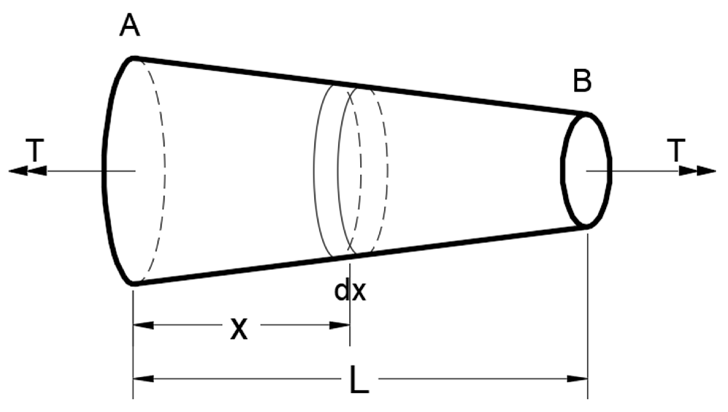
From the elementary strength of the material [17,18], the bar with a continuously varying cross section and constant torque is shown in Figure 1; the differential torsion angle (dθ) for the element of length (dx) is

$$d\theta ={\displaystyle \frac{Tdx}{GJ\left(x\right)}}$$

(3)

In which J(x) is the torsion constant, and equal to the polar moment of inertia (Ip) in the circular cross section.

$$\theta ={\int }_0^{L}d\theta ={\int }_o^L{\displaystyle \frac{Tdx}{GJ\left(x\right)}}$$

(4)

For continuously varying torque, T(x),

$$\theta ={\int }_o^L{\displaystyle \frac{Tdx}{GJ\left(x\right)}}$$

(5)

where

T = the applied torque (N.mm).

G = Modulus of rigidity (Shear modulus) N/mm²

J(x) = torsion constant (mm⁴).

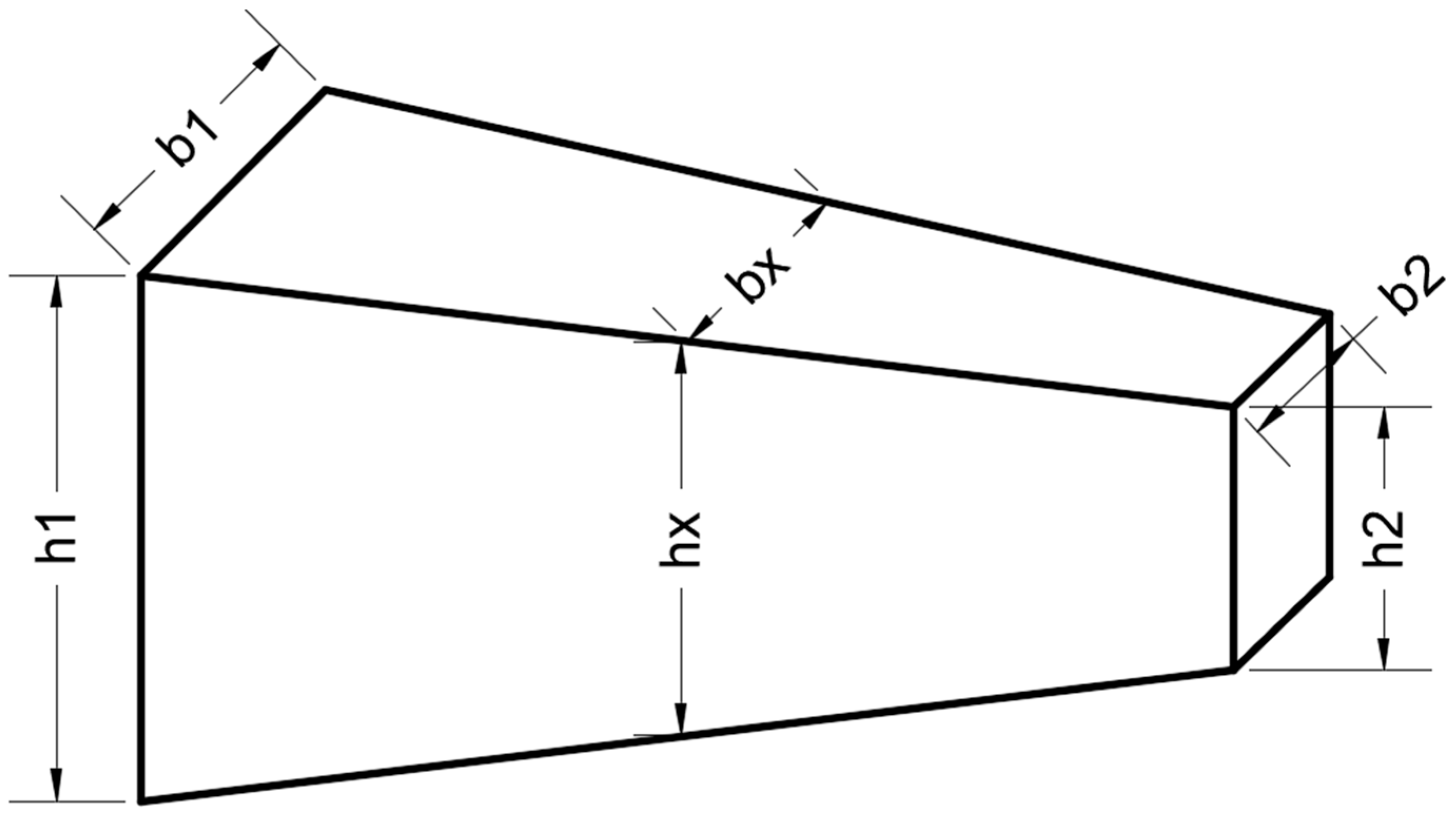
For the non-prismatic rectangular section (singly tapered cross section) shown in Figure 2, the cross-section depth (h) at (x = 0) and (h₂) at (x = L) and constant width (b₂), depth of the section is changed linearly from (h₁) to (h₂) at distance (x) and equal to

$$h_x=h_2\left[\lambda +(1-\lambda ){\displaystyle \frac{x}{L}}\right]$$

(6)

where the tapered ratio of the bar λ = h₁/h₂ ≥ 1.0.

$$\theta ={\displaystyle \frac{T}{G{b_2}^3{h}_2}}{\int }_o^L{\displaystyle \frac{dx}{\left\{\lambda +(1-\lambda )\frac{x}{L}\right\}\left[\frac{1}{3}-\frac{0.21\alpha }{\lambda +\left(1-\lambda \right)\frac{x}{L}}(1-\frac{{\alpha }^4}{12{\left\{\lambda +\left(1-\lambda \right)\frac{x}{L}\right\}}^4})\right]}}$$

(7)

where α = aspect ratio of the smallest cross section = b₂/h₂.

Using non-dimensional coordinates,

Let $\xi ={\displaystyle \frac{x}{L}};dx=Ld\xi$

The above integration becomes

$$\theta ={\displaystyle \frac{T}{G{b_2}^3{h}_2}}{\int }_o^1{\displaystyle \frac{d\xi }{\left\{\lambda +(1-\lambda )\xi \right\}\left[\frac{1}{3}-\frac{0.21\alpha }{\lambda +\left(1-\lambda \right)\xi }(1-\frac{{\alpha }^4}{12{\left\{\lambda +\left(1-\lambda \right)\xi \right\}}^4})\right]}}$$

(8)

Or in the following form:

$$\theta ={\displaystyle \frac{TL}{GJ\left(x\right)}}$$

(9)

$$J\left(x\right)={\displaystyle \frac{{b_2}^3{h}_2}{I\left(x\right)}}=f{b_2}^3{h}_2$$

(10)

$$I(x)={\int }_o^L{\displaystyle \frac{d\xi }{\left\{\lambda +(1-\lambda )\xi \right\}\left[\frac{1}{3}-\frac{0.21\alpha (1-\frac{{\alpha }^4}{12{\left\{\lambda +\left(1-\lambda \right)\xi \right\}}^4})}{\{\lambda +\left(1-\lambda \right)\xi \}}\right]}}$$

(11)

where f = (Torsion constant coefficient) =${\displaystyle \frac{1}{I\left(x\right)}}$.

The above integral I(x) is performed by numerical integration method (Trapezoidal rule method) for different values of the cross-section aspect ratio (α) and tapered ratio of the bar (λ) and shown in

Table A1. Dimensionless integral I(x) as a function of section aspect ratio α = b₂/h₂ and depth-taper ratio λ_h = h₁/h₂ (constant width, λ_b = 1.0). Normalization: J(x)/(b₂³h₂) = 1/I(x).

α	λh = 1	λh = 1.25	λh = 1.5	λh = 1.75	λh = 2	λh = 3	λh = 4	λh = 5	λh = 10	λh = 1	λh = 100	λh = 1000
0	3.0019	2.6792	2.4341	2.2396	2.0804	1.8334	1.6486	1.3868	1.2076	0.7679	0.1419	0.0301
0.01	3.0190	2.6929	2.4455	2.2493	2.0890	1.8402	1.6543	1.3911	1.2110	0.7697	0.1421	0.0302
0.10	3.2017	2.8380	2.5658	2.3521	2.1787	1.9117	1.7137	1.4356	1.2465	0.7874	0.1441	0.0311
0.25	3.5606	3.1181	2.7954	2.5467	2.3475	2.0452	1.8241	1.5176	1.3117	0.8197	0.1479	0.0330
0.50	4.3691	3.7283	3.2852	2.9557	2.6986	2.3188	2.0482	1.6822	1.4418	0.8832	0.1555	0.0371
0.75	5.5560	4.5934	3.9626	3.5115	3.1694	2.6792	2.3401	1.8935	1.6075	0.9630	0.1655	0.0431
1.00	7.1006	5.7525	4.8662	4.2465	3.7872	3.1463	2.7151	2.1622	1.8167	1.0625	0.1778	0.0509

, and the results of the torsion constant coefficient (f) in

Table A2. Normalized torsional constant J(x)/(b₂³h₂) as a function of section aspect ratio α = b₂/h₂ and depth-taper ratio λ_h = h₁/h₂ (constant width, λ_b = 1.0). Note: J(x)/(b₂³h₂) = 1/I(x).

α	λh = 1	λh = 1.25	λh = 1.5	λh = 1.75	λh = 2	λh = 3	λh = 4	λh = 5	λh = 10	λh = 1	λh = 100	λh = 1000
0	0.3331	0.3732	0.4108	0.4465	0.4807	0.5454	0.6066	0.7211	0.8281	1.3022	7.0488	33.2070
0.01	0.3312	0.3713	0.4089	0.4446	0.4787	0.5434	0.6045	0.7189	0.8258	1.2993	7.0391	33.1101
0.10	0.3123	0.3524	0.3897	0.4252	0.4590	0.5231	0.5835	0.6966	0.8023	1.2701	6.9398	32.1130
0.25	0.2809	0.3207	0.3577	0.3927	0.4260	0.4889	0.5482	0.6589	0.7623	1.2200	6.7634	30.3255
0.50	0.2289	0.2682	0.3044	0.3383	0.3706	0.4313	0.4882	0.5945	0.6936	1.1322	6.4317	26.9632
0.75	0.1800	0.2177	0.2524	0.2848	0.3155	0.3732	0.4273	0.5281	0.6221	1.0384	6.0438	23.2056
1.00	0.1408	0.1738	0.2055	0.2355	0.2640	0.3178	0.3683	0.4625	0.5504	0.9412	5.6245	19.6508

.

To anchor Equation (11) with design-ready numbers,

Table 1. Singly tapered member (λ_b = 1): representative values of the torsion coefficient f = J/(b₂³h₂) for α ∈ {0.10, 0.50, 1.00}, and λ ∈ {1, 2, 3, 5} (extracted from the full grids in Appendix A).

α	λ = 1	λ = 2	λ = 3	λ = 5
0.10	0.3123	0.4590	0.5835	0.8023
0.50	0.2289	0.3706	0.4882	0.6936
1.00	0.1408	0.2640	0.3683	0.5504

Notes: α = b₂/h₂ (section aspect ratio at the smaller end); λ = h₁/h₂ (depth-taper ratio); λ_b = b₁/b₂ (width-taper ratio, equal to 1 here). Full numeric tables remain in Appendix A; trend plots are in Appendix B.

summarizes representative values of the non-dimensional torsion coefficient f = J/(b₂³h₂) for the singly tapered case (λ_b = 1). The subset spans α ∈ {0.10, 0.50, 1.00} and λ ∈ {1, 2, 3, 5}.

Consistent with the full grids in Appendix A (and trends in Appendix B), f increases monotonically with λ at fixed α and decreases as α increases; for example, for α = 1.00, it rises from 0.1408 at λ = 1 to 0.5504 at λ = 5. For preliminary sizing, select α and λ from the target geometry, read f in Table 1, and compute J = fb₂³h₂.

For non-prismatic bars (doubly tapered cross section) shown in Figure 3, when both dimensions (b and h) are changed linearly with the longitudinal axis of the bar.

$$b_x=h_2[{\lambda }_h\left(1-{\lambda }_h\right){\displaystyle \frac{x}{L}}]$$

(12)

$$b_x=b_2[{\lambda }_h\left(1-{\lambda }_b\right){\displaystyle \frac{x}{L}}]$$

(13)

where

λ_h = tapered depth ratio = h₁/h₂ ≥ 1.0

λ_b = tapered width ratio = b₁/b₂ ≥ 1.0

The equation of the rotation can be written by some previous integral as the following:

$$\theta ={\displaystyle \frac{TL}{GJ\left(x\right)}}$$

(9)

$$J\left(x\right)={\displaystyle \frac{{b_2}^3{h}_2}{I\left(x\right)}}$$

(10)

where

$$I(x)={\int }_0^1{\displaystyle \frac{d\xi }{\{{\lambda }_h+(1-{\lambda }_h)\xi \}\{{\lambda }_b+(1-{\lambda }_b)\xi \}[\frac{1}{3}-0.21\alpha \frac{\left\{{\lambda }_b+\left(1-{\lambda }_b\right)\xi \right\}}{\left\{{\lambda }_h+\left(1-{\lambda }_h\right)\xi \right\}}\left\{1-\frac{{\alpha }^4}{12}{\left(\frac{{\lambda }_b+\left(1-{\lambda }_b\right)\xi }{{\lambda }_h+\left(1-{\lambda }_h\right)\xi }\right)}^4\right\}]}}$$

(14)

$\alpha =$ cross section aspect ratio of the smallest cross section =${\displaystyle \frac{b_2}{h_2}}$.

To operationalize Equations (12)–(14) for the doubly tapered case,

Table 2. Doubly tapered member (λ_b = 3): representative values of the torsion coefficient f = J/(b₂³h₂) for α ∈ {0.50, 1.00} and λ_h ∈ {1, 2, 5, 10} (extracted from the full grids in Appendix A).

α	λh = 1	λh = 2	λh = 5	λh = 10
0.50	0.8098	1.1603	1.8425	2.6522
1.00	0.7625	0.7154	1.2295	1.9284

summarizes representative values of the non-dimensional torsion coefficient f = J/(b₂³h₂) with width taper fixed at λ_b = 3. The subset spans α ∈ {0.50, 1.00} and depth-taper ratios λ_h ∈ {1, 2, 5, 10}.

Consistent with the full grids in Appendix A and the trend plots in Appendix B, when the width taper is fixed at λ_b = 3, the normalized torsional coefficient f = J/(b₂³h₂) increases with the depth-taper ratio λ_h. For α = 0.50, f grows monotonically from 0.8098 → 1.1603 → 1.8425 → 2.6522 as λ_h = 1→2→5→10 (i.e., 0.8098 → 2.6522 overall). For α =1.00, a mild non-monotonicity occurs near λ_h = 2: f dips from 0.7625 (λ_h = 1) to 0.7154 (λ_h = 2) before rising to 1.2295 (λ_h = 5) and 1.9284 (λ_h = 10). These summary values appear in Table 2 and show that, beyond λ_h ≈ 2, the depth-taper effect dominates and f resumes an upward trajectory. For quick design, select (α, λ_b, λ_h), read f from Table 2, and consult Appendix A for the complete tables. Notes: α = b₂/h₂ (aspect ratio at the smaller end); λ_h =λ₁/λ₂ (depth-taper ratio); λ_b =b₁/b₂ (width-taper ratio, fixed at 3 here). f is dimensionless. Full numeric grids are provided in Appendix A.

The results of the above integral I(x) performed for different values of tapered depth and width ratios (λ_h, λ_b) and cross-section aspect ratio (α) are shown in

Table A3. Dimensionless integral I(x) versus section aspect ratio α = b₂/h₂ for selected depth-taper ratios λ_h = h₁/h₂ (constant width, λ_b = 1.0). Normalization: J(x)/(b₂³h₂) = 1/I(x).

α	λh = 1	λh = 1.25	λh = 1.5	λh = 1.75	λh = 2	λh = 3	λh = 4	λh = 5	λh = 10
0.000	3.0000	2.6777	2.4328	2.2385	2.0795	1.6480	1.3864	1.2072	0.7678
0.001	3.0019	2.6792	2.4341	2.2396	2.0804	1.6486	1.3868	1.2076	0.7679
0.010	3.0190	2.6929	2.4455	2.2493	2.0890	1.6543	1.3911	1.2110	0.7697
0.100	3.2017	2.8380	2.5658	2.3521	2.1787	1.7137	1.4356	1.2465	0.7874
0.250	3.5606	3.1181	2.7954	2.5467	2.3475	1.8241	1.5176	1.3117	0.8197
0.500	4.3691	3.7283	3.2852	2.9557	2.6986	2.0482	1.6822	1.4418	0.8832
0.750	5.5560	4.5934	3.9626	3.5115	3.1694	2.3401	1.8935	1.6075	0.9630
1.000	7.1006	5.7525	4.8662	4.2465	3.7872	2.7151	2.1622	1.8167	1.0625

,

Table A4. Dimensionless integral I(x) versus section aspect ratio α = b₂/h₂ for selected depth-taper ratios λ_h = h₁/h₂ (constant width, λ_b = 1.25). Normalization: J(x)/(b₂³h₂) = 1/I(x).

α	λh = 1	λh = 1.25	λh = 1.5	λh = 1.75	λh = 2	λh = 3	λh = 4	λh = 5	λh = 10
0.000	2.1600	1.9520	1.7915	1.6624	1.5556	1.2599	1.0758	0.9473	0.6223
0.001	2.1615	1.9532	1.7925	1.6633	1.5564	1.2604	1.0762	0.9476	0.6224
0.250	2.6184	2.3168	2.0952	1.9231	1.7842	1.4139	1.1924	1.0414	0.6706
0.500	3.3120	2.8429	2.5199	2.2798	2.0921	1.6141	1.3414	1.1603	0.7303
0.750	4.3589	3.6151	3.1270	2.7795	2.5168	1.8806	1.5364	1.3143	0.8061
1.000	5.5094	4.6202	3.9386	3.4479	3.0822	2.2282	1.7875	1.5112	0.9015

,

Table A5. Dimensionless integral I(x) versus section aspect ratio α = b₂/h₂ for selected depth-taper ratios λ_h = h₁/h₂ (constant width, λ_b = 1.5). Normalization: J(x)/(b₂³h₂) = 1/I(x).

α	λh = 1	λh = 1.25	λh = 1.5	λh = 1.75	λh = 2	λh = 3	λh = 4	λh = 5	λh = 10
0	1.6667	1.5212	1.4075	1.3150	1.2378	1.0202	0.8816	0.7834	0.5283
0.25	2.0563	1.8344	1.6705	1.5424	1.4385	1.1581	0.9875	0.8696	0.5738
0.50	2.6716	2.3024	2.0498	1.8623	1.7157	1.3408	1.1249	0.9801	0.6305
0.75	3.5922	3.0055	2.6066	2.3221	2.1074	1.5887	1.3075	1.1253	0.7032
1.00	4.2432	3.8281	3.3312	2.9350	2.6316	1.9157	1.5454	1.3127	0.7953

,

Table A6. Dimensionless integral I(x) versus section aspect ratio α = b₂/h₂ for selected depth-taper ratios λ_h = h₁/h₂ (constant width, λ_b = 1.75). Normalization: J(x)/(b₂³h₂) = 1/I(x).

α	λh = 1	λh = 1.25	λh = 1.5	λh = 1.75	λh = 2	λh = 3	λh = 4	λh = 5	λh = 10
0	1.3470	1.2395	1.1544	1.0846	1.0259	0.8578	0.7488	0.6704	0.4621
0.25	1.6870	1.5149	1.3874	1.2873	1.2057	0.9834	0.8462	0.7504	0.5052
0.50	2.2445	1.9404	1.7330	1.5796	1.4598	1.1526	0.9745	0.8542	0.5595
0.75	3.0212	2.5825	2.2501	2.0087	1.8263	1.3861	1.1475	0.9923	0.6296
1.00	3.2508	3.1753	2.8747	2.5671	2.3137	1.6965	1.3747	1.1720	0.7190

,

Table A7. Dimensionless integral I(x) versus section aspect ratio α = b₂/h₂ for selected depth-taper ratios λ_h = h₁/h₂ (constant width, λ_b = 2.0). Normalization: J(x)/(b₂³h₂) = 1/I(x).

α	λh = 1	λh = 1.25	λh = 1.5	λh = 1.75	λh = 2	λh = 3	λh = 4	λh = 5	λh = 10
0	1.1251	1.0423	0.9762	0.9215	0.8751	0.7407	0.6520	0.5875	0.4126
0.25	1.4277	1.2890	1.1860	1.1050	1.0386	0.8564	0.7427	0.6624	0.4537
0.50	1.9390	1.6814	1.5055	1.3757	1.2745	1.0148	0.8635	0.7607	0.5059
0.75	2.5505	2.2601	1.9876	1.7796	1.6207	1.2367	1.0286	0.8930	0.5739
1.00	2.5531	2.6163	2.4897	2.2766	2.0712	1.5330	1.2469	1.0663	0.6609

,

Table A8. Dimensionless integral I(x) versus section aspect ratio α = b₂/h₂ for selected depth-taper ratios λ_h = h₁/h₂ (constant width, λ_b = 3.0). Normalization: J(x)/(b₂³h₂) = 1/I(x).

α	λh = 1	λh = 1.25	λh = 1.5	λh = 1.75	λh = 2	λh = 3	λh = 4	λh = 5	λh = 10
0	0.6668	0.6294	0.5986	0.5725	0.5499	0.4817	0.4343	0.3985	0.2955
0.25	0.8809	0.8067	0.7517	0.7082	0.6723	0.5717	0.5067	0.4596	0.3309
0.50	1.2348	1.1102	1.0049	0.9246	0.8618	0.7015	0.6075	0.5427	0.3770
0.75	1.4086	1.3917	1.3299	1.2386	1.1463	0.8921	0.7509	0.6587	0.4385
1.00	1.3115	1.3678	1.4091	1.4220	1.3977	1.1401	0.9426	0.8134	0.5186

,

Table A9. Dimensionless integral I(x) versus section aspect ratio α = b₂/h₂ for selected depth-taper ratios λ_h = h₁/h₂ (constant width, λ_b = 4.0). Normalization: J(x)/(b₂³h₂) = 1/I(x).

α	λh = 1	λh = 1.25	λh = 1.5	λh = 1.75	λh = 2	λh = 3	λh = 4	λh = 5	λh = 10
0	0.4690	0.4477	0.4298	0.4144	0.4008	0.3587	0.3284	0.3050	0.2344
0.25	0.6377	0.5887	0.5526	0.5240	0.5005	0.4337	0.3898	0.3574	0.2660
0.50	0.8593	0.8160	0.7608	0.7078	0.6632	0.5467	0.4783	0.4310	0.3080
0.75	0.9444	0.9458	0.9370	0.9151	0.8800	0.7166	0.6082	0.5368	0.3651
1.00	0.8757	0.9027	0.9274	0.9476	0.9607	0.9055	0.7773	0.6776	0.4402

,

Table A10. Dimensionless integral I(x) versus section aspect ratio α = b₂/h₂ for selected depth-taper ratios λ_h = h₁/h₂ (constant width, λ_b = 5.0). Normalization: J(x)/(b₂³h₂) = 1/I(x).

α	λh = 1	λh = 1.25	λh = 1.5	λh = 1.75	λh = 2	λh = 3	λh = 4	λh = 5	λh = 10
0	0.3603	0.3466	0.3348	0.3246	0.3155	0.2866	0.2653	0.2484	0.1960
0.25	0.4999	0.4649	0.4385	0.4176	0.4004	0.3516	0.3191	0.2948	0.2248
0.50	0.6483	0.6292	0.6038	0.5736	0.5431	0.4531	0.3991	0.3618	0.2637
0.75	0.7089	0.7108	0.7093	0.7033	0.6920	0.6037	0.5189	0.4600	0.3175
1.00	0.6571	0.6725	0.6873	0.7007	0.7123	0.7217	0.6615	0.5879	0.3889

and

Table A11. Dimensionless integral I(x) versus section aspect ratio α = b₂/h₂ for selected depth-taper ratios λ_h = h₁/h₂ (constant width, λ_b = 10). Normalization: J(x)/(b₂³h₂) = 1/I(x)

α	λh = 1	λh = 1.25	λh = 1.5	λh = 1.75	λh = 2	λh = 3	λh = 4	λh = 5	λh = 10
0	0.1657	0.1622	0.1590	0.1562	0.1536	0.1448	0.1378	0.1319	0.1119
0.25	0.2314	0.2249	0.2182	0.2115	0.2051	0.1859	0.1729	0.1630	0.1328
0.50	0.2892	0.2861	0.2825	0.2786	0.2742	0.2533	0.2308	0.2125	0.1630
0.75	0.3159	0.3165	0.3168	0.3169	0.3167	0.3121	0.3005	0.2828	0.2072
1.00	0.2930	0.2961	0.2991	0.3022	0.3051	0.3157	0.3232	0.3255	0.2648

and the results of the torsion constant coefficient J(x)/b₂³ h₂ are shown in

Table A12. Normalized torsional constant J(x)/(b₂³h₂) versus section aspect ratio α = b₂/h₂ for selected depth-taper ratios λ_h = h₁/h₂ (constant width, λ_b = 1.0). Normalization: J(x)/(b₂³h₂) = 1/I(x).

α	λh = 1	λh = 1.25	λh = 1.5	λh = 1.75	λh = 2	λh = 3	λh = 4	λh = 5	λh = 10
0	0.3333	0.3735	0.4110	0.4467	0.4809	0.6068	0.7213	0.8284	1.3025
0.001	0.3331	0.3732	0.4108	0.4465	0.4807	0.6066	0.7211	0.8281	1.3022
0.010	0.3312	0.3713	0.4089	0.4446	0.4787	0.6045	0.7189	0.8258	1.2993
0.100	0.3123	0.3524	0.3897	0.4252	0.4590	0.5835	0.6966	0.8023	1.2701
0.250	0.2809	0.3207	0.3577	0.3927	0.4260	0.5482	0.6589	0.7623	1.2200
0.500	0.2289	0.2682	0.3044	0.3383	0.3706	0.4882	0.5945	0.6936	1.1322
0.750	0.1800	0.2177	0.2524	0.2848	0.3155	0.4273	0.5281	0.6221	1.0384
1.000	0.1408	0.1738	0.2055	0.2355	0.2640	0.3683	0.4625	0.5504	0.9412

,

Table A13. Normalized torsional constant J(x)/(b₂³h₂) versus section aspect ratio α = b₂/h₂ for selected depth-taper ratios λ_h = h₁/h₂ (constant width, λ_b = 1.25). Normalization: J(x)/(b₂³h₂) = 1/I(x).

α	λh = 1	λh = 1.25	λh = 1.5	λh = 1.75	λh = 2	λh = 3	λh = 4	λh = 5	λh = 10
0	0.4630	0.5123	0.5582	0.6015	0.6428	0.7937	0.9295	1.0556	1.6070
0.001	0.4626	0.5120	0.5579	0.6012	0.6425	0.7934	0.9292	1.0553	1.6066
0.250	0.3819	0.4316	0.4773	0.5200	0.5605	0.7073	0.8386	0.9603	1.4913
0.500	0.3019	0.3518	0.3968	0.4386	0.4780	0.6195	0.7455	0.8619	1.3693
0.750	0.2294	0.2766	0.3198	0.3598	0.3973	0.5317	0.6509	0.7609	1.2405
1.000	0.1815	0.2164	0.2539	0.2900	0.3244	0.4488	0.5594	0.6617	1.1093

,

Table A14. Normalized torsional constant J(x)/(b₂³h₂) versus section aspect ratio α = b₂/h₂ for selected depth-taper ratios λ_h = h₁/h₂ (constant width, λ_b = 1.5). Normalization: J(x)/(b₂³h₂) = 1/I(x).

α	λh = 1	λh = 1.25	λh = 1.5	λh = 1.75	λh = 2	λh = 3	λh = 4	λh = 5	λh = 10
0	0.6000	0.6574	0.7105	0.7605	0.8079	0.9802	1.1342	1.2765	1.8928
0.25	0.4863	0.5451	0.5986	0.6483	0.6952	0.8635	1.0126	1.1499	1.7429
0.50	0.3743	0.4343	0.4879	0.5370	0.5829	0.7458	0.8890	1.0203	1.5860
0.75	0.2784	0.3327	0.3836	0.4307	0.4745	0.6294	0.7648	0.8887	1.4220
1.00	0.2357	0.2612	0.3002	0.3407	0.3800	0.5220	0.6471	0.7618	1.2574

,

Table A15. Normalized torsional constant J(x)/(b₂³h₂) versus section aspect ratio α = b₂/h₂ for selected depth-taper ratios λ_h = h₁/h₂ (constant width, λ_b = 1.75). Normalization: J(x)/(b₂³h₂) = 1/I(x).

α	λh = 1	λh = 1.25	λh = 1.5	λh = 1.75	λh = 2	λh = 3	λh = 4	λh = 5	λh = 10
0	0.7424	0.8068	0.8663	0.9220	0.9748	1.1657	1.3355	1.4917	2.1640
0.25	0.5928	0.6601	0.7208	0.7768	0.8294	1.0169	1.1817	1.3327	1.9794
0.50	0.4455	0.5154	0.5770	0.6331	0.6850	0.8676	1.0262	1.1707	1.7873
0.75	0.3310	0.3872	0.4444	0.4978	0.5476	0.7214	0.8715	1.0078	1.5882
1.00	0.3076	0.3149	0.3479	0.3895	0.4322	0.5894	0.7275	0.8532	1.3909

,

Table A16. Normalized torsional constant J(x)/(b₂³h₂) versus section aspect ratio α = b₂/h₂ for selected depth-taper ratios λ_h = h₁/h₂ (constant width, λ_b = 2.0). Normalization: J(x)/(b₂³h₂) = 1/I(x).

α	λh = 1	λh = 1.25	λh = 1.5	λh = 1.75	λh = 2	λh = 3	λh = 4	λh = 5	λh = 10
0	0.8888	0.9594	1.0244	1.0852	1.1427	1.3501	1.5337	1.7022	2.4237
0.25	0.7004	0.7758	0.8432	0.9050	0.9628	1.1676	1.3465	1.5097	2.2040
0.50	0.5157	0.5947	0.6642	0.7269	0.7846	0.9854	1.1580	1.3145	1.9765
0.75	0.3921	0.4425	0.5031	0.5619	0.6170	0.8086	0.9722	1.1199	1.7426
1.00	0.3917	0.3822	0.4016	0.4393	0.4828	0.6523	0.8020	0.9378	1.5132

,

Table A17. Normalized torsional constant J(x)/(b₂³h₂) versus section aspect ratio α = b₂/h₂ for selected depth-taper ratios λ_h = h₁/h₂ (constant width, λ_b = 3.0). Normalization: J(x)/(b₂³h₂) = 1/I(x).

α	λh = 1	λh = 1.25	λh = 1.5	λh = 1.75	λh = 2	λh = 3	λh = 4	λh = 5	λh = 10
0	1.4997	1.5888	1.6705	1.7466	1.8185	2.0761	2.3025	2.5092	3.3840
0.25	1.1352	1.2396	1.3303	1.4120	1.4874	1.7492	1.9736	2.1759	3.0217
0.50	0.8098	0.9008	0.9951	1.0816	1.1603	1.4255	1.6462	1.8425	2.6522
0.75	0.7099	0.7185	0.7519	0.8074	0.8724	1.1210	1.3317	1.5181	2.2805
1.00	0.7625	0.7311	0.7097	0.7032	0.7154	0.8771	1.0609	1.2295	1.9284

,

Table A18. Normalized torsional constant J(x)/(b₂³h₂) versus section aspect ratio α = b₂/h₂ for selected depth-taper ratios λ_h = h₁/h₂ (constant width, λ_b = 4.0). Normalization: J(x)/(b₂³h₂) = 1/I(x).

α	λh = 1	λh = 1.25	λh = 1.5	λh = 1.75	λh = 2	λh = 3	λh = 4	λh = 5	λh = 10
0	2.1323	2.2336	2.3266	2.4132	2.4950	2.7878	3.0448	3.2791	4.2662
0.25	1.5682	1.6986	1.8097	1.9083	1.9982	2.3056	2.5654	2.7980	3.7591
0.50	1.1637	1.2255	1.3144	1.4128	1.5079	1.8292	2.0907	2.3199	3.2469
0.75	1.0589	1.0574	1.0673	1.0928	1.1363	1.3956	1.6441	1.8630	2.7393
1.00	1.1420	1.1078	1.0783	1.0553	1.0409	1.1043	1.2864	1.4757	2.2715

,

Table A19. Normalized torsional constant J(x)/(b₂³h₂) versus section aspect ratio α = b₂/h₂ for selected depth-taper ratios λ_h = h₁/h₂ (constant width, λ_b = 5.0). Normalization: J(x)/(b₂³h₂) = 1/I(x).

α	λh = 1	λh = 1.25	λh = 1.5	λh = 1.75	λh = 2	λh = 3	λh = 4	λh = 5	λh = 10
0	2.7755	2.8854	2.9865	3.0808	3.1699	3.4893	3.7700	4.0258	5.1020
0.25	2.0003	2.1510	2.2807	2.3946	2.4975	2.8444	3.1342	3.3919	4.4484
0.50	1.5424	1.5893	1.6561	1.7432	1.8413	2.2071	2.5057	2.7643	3.7923
0.75	1.4107	1.4068	1.4099	1.4219	1.4451	1.6565	1.9271	2.1737	3.1499
1.00	1.5219	1.4869	1.4550	1.4271	1.4039	1.3856	1.5118	1.7009	2.5715

and

Table A20. Normalized torsional constant J(x)/(b₂³h₂) versus section aspect ratio α = b₂/h₂ for selected depth-taper ratios λ_h = h₁/h₂ (constant width, λ_b = 10.0). Normalization: J(x)/(b₂³h₂) = 1/I(x).

α	λh = 1	λh = 1.25	λh = 1.5	λh = 1.75	λh = 2	λh = 3	λh = 4	λh = 5	λh = 10
0	6.0360	6.1668	6.2884	6.4030	6.5119	6.9069	7.2577	7.5791	8.9368
0.25	4.3222	4.4456	4.5821	4.7284	4.8747	5.3787	5.7834	6.1344	7.5297
0.50	3.4576	3.4957	3.5395	3.5896	3.6465	3.9482	4.3329	4.7058	6.1364
0.75	3.1660	3.1599	3.1564	3.1557	3.1580	3.2045	3.3274	3.5361	4.8255
1.00	3.4135	3.3776	3.3430	3.3096	3.2776	3.1671	3.0936	3.0726	3.7758

.

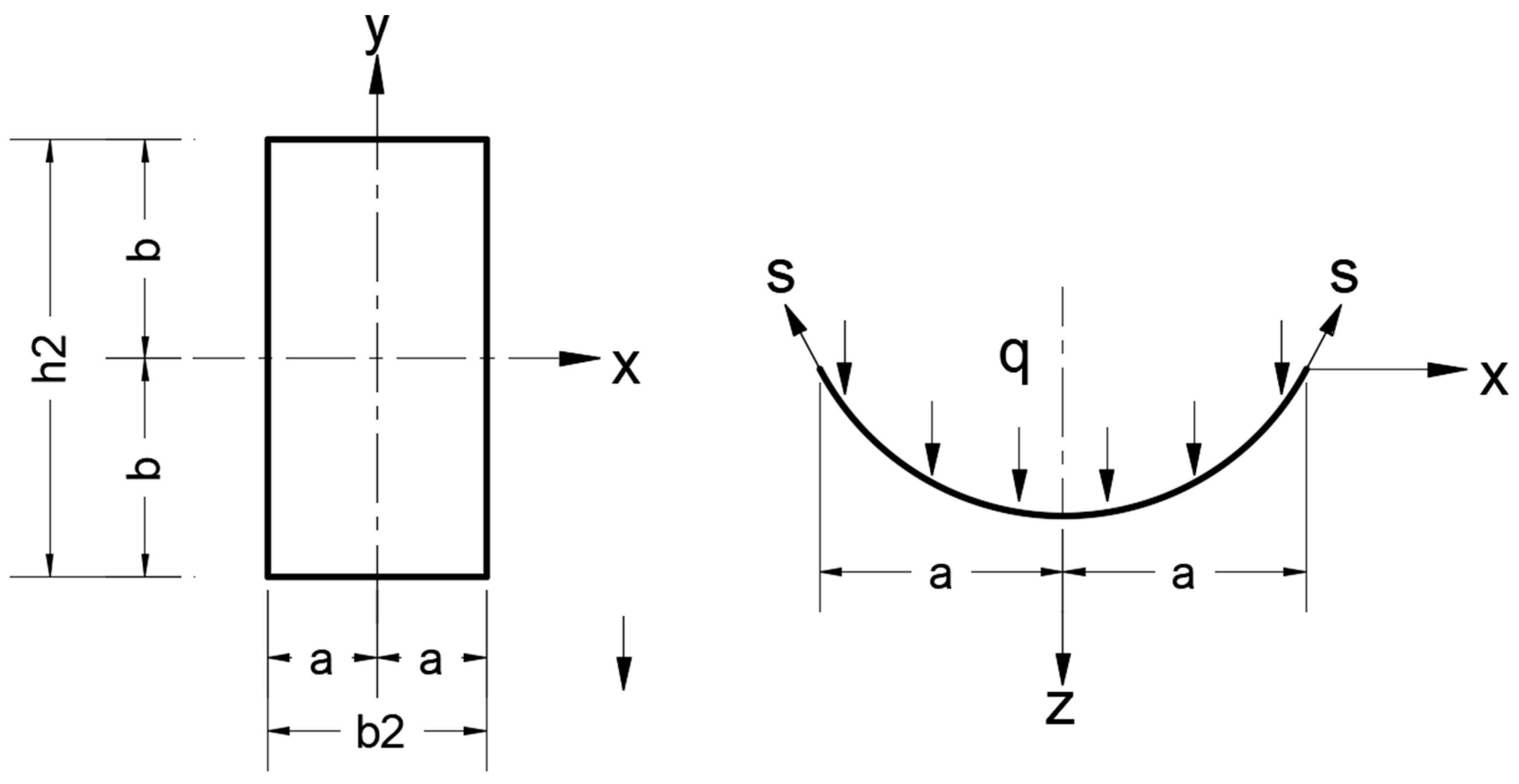
In membrane analogy analysis based on theory of elasticity principles [9,19,20,21,22,23] using the membrane analogy, the problem reduces to finding the deflection of a uniformly loaded rectangular membrane shown in Figure 4, and the deflections must satisfy the following equation:

$${\displaystyle \frac{{𝜕}^{2}z}{{𝜕x}^2}}+{\displaystyle \frac{{𝜕}^{2}z}{{𝜕y}^2}}=-{\displaystyle \frac{q}{s}}$$

(15)

The problem is symmetry about axis y; at the sides x = ±a, the above equation can be satisfied taking the following deflection function:

$$z=\sum _{n=\mathrm{1,3},5}^{\infty }{Y}_{n}cos{\displaystyle \frac{n\pi x}{2a}}$$

(16)

where

z = the equation of the deflection function which is satisfied by the boundary conditions of the membrane and in the torsion problem, represents the stress function ($\varnothing$).

q = transverse load on the membrane (N/mm²).

s = the tension in-plane force developed in the membrane (N/mm).

Subsisting z into Equation (15) and representing (q/s) in the form of Fourier series, the following differential equation is obtained:

$${Y_n}^{II}-{\displaystyle \frac{n^2{\pi }^2}{4a^2}}{Y}_n=-{\displaystyle \frac{q}{s}}{\displaystyle \frac{4}{n\pi B_n}}{(-1)}^{{\displaystyle \frac{n-1}{2}}}$$

(17)

The general solution of this differential equation is

$$Y_n=Ansinh{\displaystyle \frac{n\pi y}{2a}}+Bncosh{\displaystyle \frac{n\pi y}{2a}}+{\displaystyle \frac{16q{a}^2}{s{n}^3{\pi }^3{B}_n}}{(-1)}^{{\displaystyle \frac{n-1}{2}}}$$

(18)

An and Bn are constants and determined from the boundary conditions.

Due to symmetry about x-axis, the constant (A) must be zero, and at y = ± b, Y_n = 0, the constant B is determined, thus (q/s = 2GA).

The final form of (z) or stress function (ϕ) is

$$\varphi ={\displaystyle \frac{32G\theta a^2}{{\pi }^3}}\sum _{n=1,\mathrm{3,5}}^{\infty }{\displaystyle \frac{{(-1)}^{\frac{n-1}{2}}}{n^3}}[1-{\displaystyle \frac{cosh(\frac{n\pi y}{2a})}{cosh(\frac{n\pi b}{2a})}}]\mathit{cos}{\displaystyle \frac{n\pi x}{2a}}$$

(19)

Equation (19) represents the final form of Equation (17) which is the general equation of the membrane or torsion stress function.

The shear stress τ_yz = −∂ϕ/∂x

$${\tau }_{yz}={\displaystyle \frac{16G\theta a^2}{{\pi }^2}}\sum _{n=1,3,5}^{\infty }{\displaystyle \frac{{(-1)}^{\frac{n-1}{2}}}{n^2}}[1-{\displaystyle \frac{\mathrm{c}\mathrm{o}\mathrm{s}\mathrm{h}(\frac{n\pi y}{2a})}{\mathrm{c}\mathrm{o}\mathrm{s}\mathrm{h}(\frac{n\pi b}{2a})}}]\sin {\displaystyle \frac{n\pi x}{2a}}$$

(20)

At middle plane y = 0 and x = a; the maximum stress is equal to

$${\tau }_{max}={\displaystyle \frac{16G\theta a^2}{{\pi }^2}}\sum _{n=1,3,5}^{\infty }{\displaystyle \frac{1}{n^2}}[1-{\displaystyle \frac{1}{\mathrm{c}\mathrm{o}\mathrm{s}\mathrm{h}(\frac{n\pi b}{2a})}}]$$

(21)

Taking $\sum _{\mathit{n}=\mathrm{1,3},5}^{\mathit{\infty }}{\displaystyle \frac{1}{{\mathit{n}}^2}}={\displaystyle \frac{{\mathit{\pi }}^2}{8}}$

$${\tau }_{max}=2G\theta a[1-{\displaystyle \frac{8}{{\pi }^2}}\sum {\displaystyle \frac{1}{n^{2}cosh(\frac{n\pi b}{2a})}}]$$

(22)

The torque (T) can be determined as a function of (GA):

$$T=2{\int }_{-a}^a{\int }_{-b}^b\varphi dxdy={\displaystyle \frac{GA{\left(2a\right)}^3\left(2b\right)}{3}}\left[1-{\displaystyle \frac{192a}{{\pi }^{5}b}}\sum {\displaystyle \frac{1}{n^5}}tanh{\displaystyle \frac{n\pi b}{2a}}\right]=G\theta J$$

(23)

$$\mathrm{T}\mathrm{o}\mathrm{r}\mathrm{s}\mathrm{i}\mathrm{o}\mathrm{n}\mathrm{c}\mathrm{o}\mathrm{n}\mathrm{s}\mathrm{t}\mathrm{a}\mathrm{n}\mathrm{t}(J)={\displaystyle \frac{{\left(2a\right)}^3\left(2b\right)}{3}}[1-{\displaystyle \frac{192a}{{\pi }^{5}b}}\sum {\displaystyle \frac{1}{n^5}}tanh{\displaystyle \frac{n\pi b}{2a}}]$$

(24)

Here, θ is the twisting angle per unit length.

For the rectangular cross section, (width = b₂ and depth = h₂).

$$\mathit{J}={\displaystyle \frac{{{\mathit{b}}_{\mathbf{2}}}^{\mathbf{3}}{\mathit{h}}_{\mathbf{2}}}{\mathbf{3}}}[\mathbf{1}-{\displaystyle \frac{\mathbf{192}\mathit{\alpha }}{{\mathit{\pi }}^{\mathbf{5}}\mathit{b}}}\sum {\displaystyle \frac{\mathbf{1}}{{\mathit{n}}^{\mathbf{5}}}}\mathit{t}\mathit{a}\mathit{n}\mathit{h}{\displaystyle \frac{\mathit{n}\mathit{\pi }\mathit{b}}{\mathbf{2}\mathit{\alpha }}}]$$

(25)

where b₂ = 2a, h₂ = 2b, and $\alpha ={\displaystyle \frac{b_2}{h_2}}$.

$${\mathit{\tau }}_{\mathit{m}\mathit{a}\mathit{x}}={\displaystyle \frac{\mathit{G}\mathit{\theta }{\mathit{b}}_{\mathbf{2}}}{\mathit{L}}}[\mathbf{1}-{\displaystyle \frac{\mathbf{8}}{{\mathit{\pi }}^{\mathbf{2}}}}\sum {\displaystyle \frac{\mathbf{1}}{{\mathit{n}}^{\mathbf{2}}\mathbf{cosh}\left(\frac{\mathit{n}\mathit{\pi }}{\mathbf{2}\mathit{\alpha }}\right)}}]$$

(26)

Strain energy method: the torsion problem can be solved using the strain energy method [19,20,21,22,23].

The strain energy of the twisted bar per unit length is

$$U={\displaystyle \frac{1}{2G}}\iint ({{\tau }_{xz}}^2+{{\tau }_{yz}}^2)dxdy=\iint \{{\displaystyle \frac{1}{2}}[{({\displaystyle \frac{𝜕\varphi }{𝜕x}})}^2+{({\displaystyle \frac{𝜕\varphi }{𝜕y}})}^2)-2G\theta \}dxdy$$

(27)

Ritz methods are used to solve the above equation, by assuming stress function (ϕ) in the form of double-Fourier series, which satisfy the condition of (ϕ = 0) on the boundary.

$$\varphi =\sum _{m=}^{\infty }\sum _{n=\mathrm{1,3},5}^{\infty }{A}_{mn}\cos {\displaystyle \frac{m\pi x}{2a}}\cos {\displaystyle \frac{n\pi y}{2a}}$$

(28)

Subsisting ϕ into Equation (26), and performing the integration,

$$U={\displaystyle \frac{\pi 2ab}{8}}\sum _{m=}^{\infty }\sum _{n=\mathrm{1,3},5}^{\infty }{A_{mn}}^2\left({\displaystyle \frac{m^2}{a^2}}+{\displaystyle \frac{n^2}{b^2}}\right)-2G\theta \sum _{m=}^{\infty }\sum _{n=\mathrm{1,3},5}^{\infty }{A}_{mn}{\displaystyle \frac{16ab}{mn{\pi }^2}}{(-1)}^{{\displaystyle \frac{m+n}{2}}-1}$$

(29)

Minimizing (U) with respect to the constant Amn: ${\displaystyle \frac{𝜕U}{𝜕A_{mn}}}=0$.

$$A_{mn}={\displaystyle \frac{128G\theta b^2{(-1)}^{\frac{m+n}{2}-1}}{{\pi }^{4}mn(m^2{\alpha }^2+n^2)}}$$

(30)

where

α = aspect ratio of the section = b/a.

The torque is also determined $T=2{\int }_{-a}^a{\int }_{-b}^b\varphi dxdy$.

$$T=\sum _{m=}^{\infty }\sum _{n=\mathrm{1,3},5}^{\infty }{\displaystyle \frac{4096G\theta b^{3}a}{{\pi }^6{m}^2{n}^2(m^2{\alpha }^2+n^2)}}$$

(31)

Thus, torsion constant J is equal to

$$J=\sum _{m=}^{\infty }\sum _{n=\mathrm{1,3},5}^{\infty }{\displaystyle \frac{4096b^{3}a}{{\pi }^6{m}^2{n}^2(m^2{\alpha }^2+n^2)}}$$

(32)

The maximum strain τ_max is obtained at y = 0 and x = ±a and equal to

$${\tau }_{max}=\sum _{m=}^{\infty }\sum _{n=\mathrm{1,3},5}^{\infty }{\displaystyle \frac{m^{2}n{\pi }^3}{64a^{2}b}}sin{\displaystyle \frac{n\pi }{2}}T$$

(33)

For non-prismatic bar, use J(x) for varying cross section:

Taking $\mathit{T}={\displaystyle \frac{\mathit{G}\mathit{\theta }}{\mathit{L}}}\mathit{J}(\mathit{x})$, and a $={\displaystyle \frac{{\mathit{b}}_{\mathbf{2}}}{\mathbf{2}}}$, b $={\displaystyle \frac{{\mathit{h}}_{\mathbf{2}}}{\mathbf{2}}}$.

$$\mathit{T}={\displaystyle \frac{\mathit{G}\mathit{\theta }}{\mathit{L}}}{\displaystyle \frac{{{\mathit{b}}_{\mathbf{2}}}^{\mathbf{3}}{\mathit{h}}_{\mathbf{2}}}{\mathit{I}\left(\mathit{x}\right)}}$$

Taking one term Fourier series, m = n = 1.0

$${\tau }_{max}={\displaystyle \frac{{\pi }^3}{8}}({\displaystyle \frac{h_2}{L}}){\displaystyle \frac{G\theta }{I\left(x\right)}}$$

(34)

Let β = aspect ratio of the bar = h₂/L

$${\tau }_{max}={\displaystyle \frac{{\pi }^3}{8}}\beta {\displaystyle \frac{G\theta }{I\left(x\right)}}$$

(35)

3. Parametric Results and Interpretation

3.1. Definitions, Parameters, and Data Organization

We evaluate the integral I(x) for non-prismatic rectangular members. Two geometric families are considered:

Singly tapered (depth-only taper): the depth varies linearly along the member (λ_b = 1), while the smaller-end width b₂ is constant. The parameters are the cross-section aspect ratio α = b₂/h₂ and the depth-taper ratio λ_h ≡ λ = h₁/h₂.

Doubly tapered (depth and width taper): both depth and width vary linearly, parameterized by λ_h = h₁/h₂ and λ_b = b₁/b₂, together with α = b₂/h₂. For each case, we report I(x) and the normalized torsional coefficient f = J/b₂³h₂. Singly tapered results for I(x) and f are tabulated in Table A1 and Table A2. Doubly tapered results for I(x) appear in Table A3, Table A4, Table A5, Table A6, Table A7, Table A8, Table A9, Table A10 and Table A11, and the corresponding f = J/(b₂³h₂) in Table A12, Table A13, Table A14, Table A15, Table A16, Table A17, Table A18, Table A19 and Table A20. Trend plots are provided in Appendix B.

3.2. Singly Tapered Members (λ_b = 1)

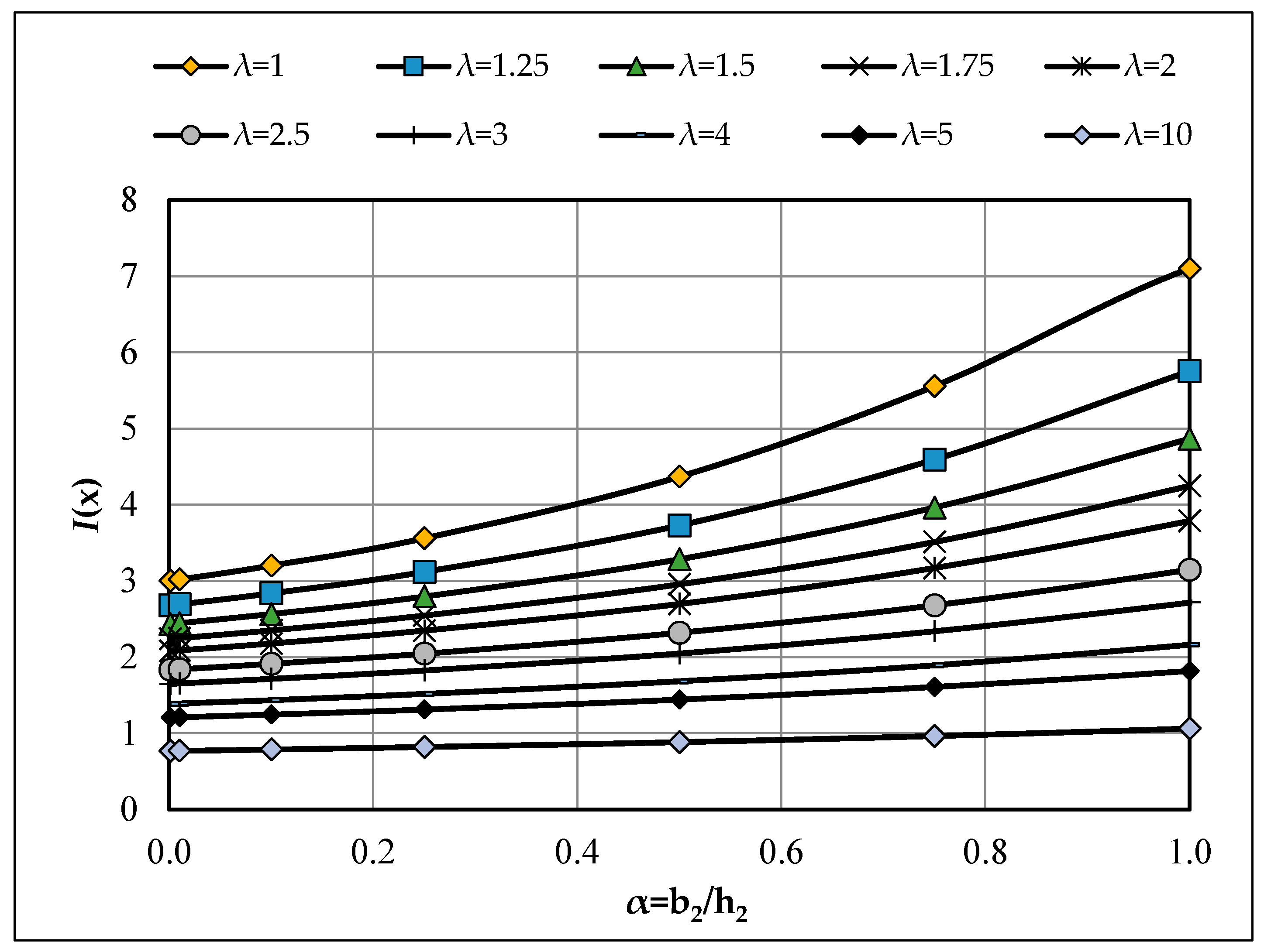
In the prismatic, very-narrow limit (α → 0, λ_h = 1), the integral tends to I (x) → 3, hence f = 1/I(x) → 1/3, reproducing the classical rectangular result. Departing from this limit, the numerical results show clear and consistent behaviors:

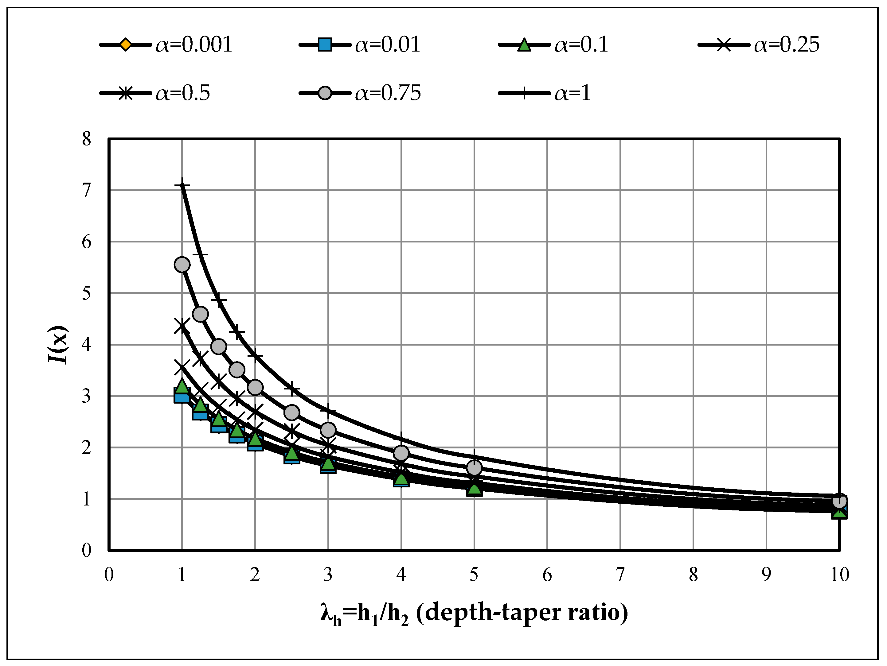
The effect of depth taper (λ_h) is as follows.: for fixed α, I(x) decreases monotonically with increasing λ_h, while f = 1/I(x) increases.

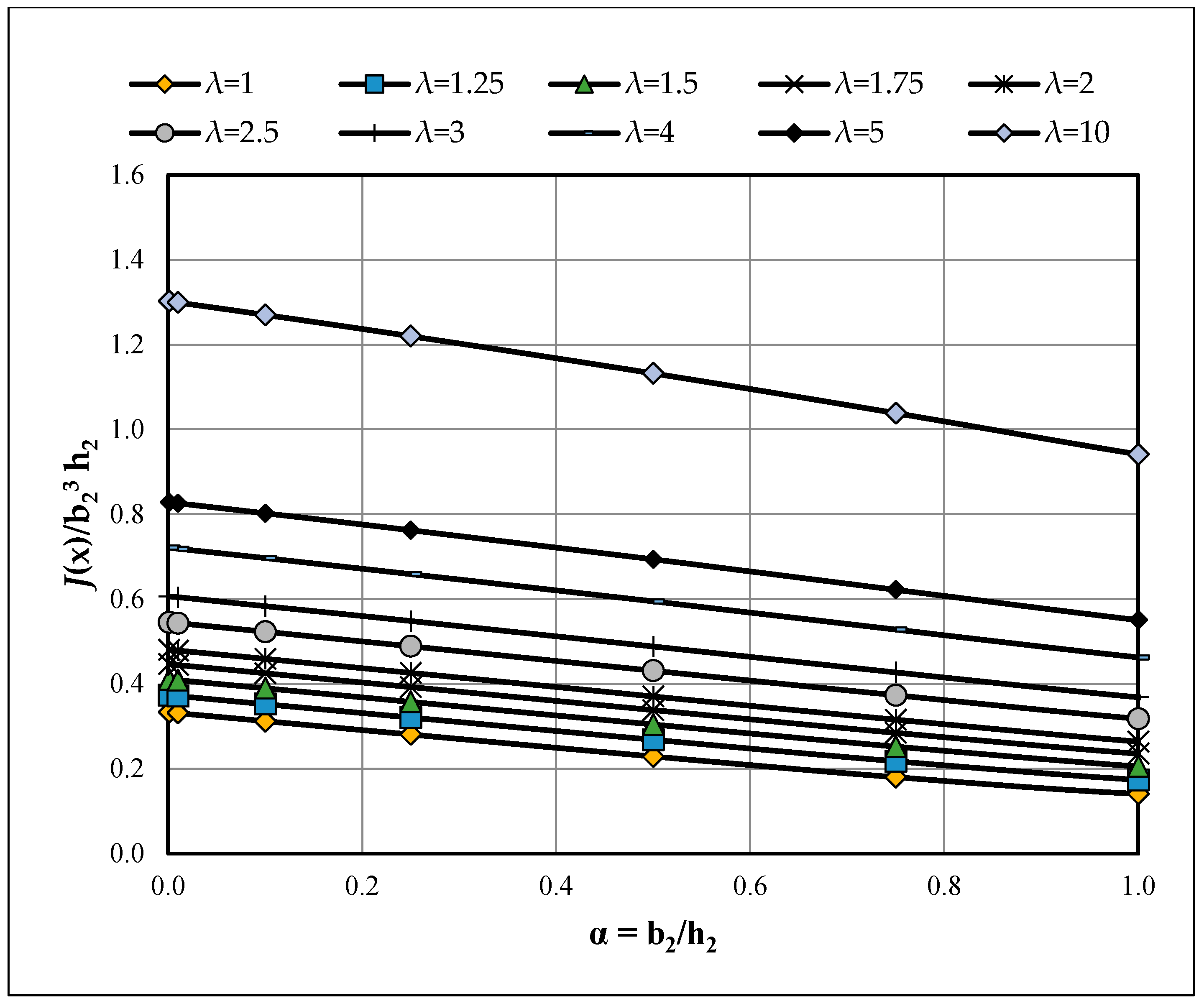
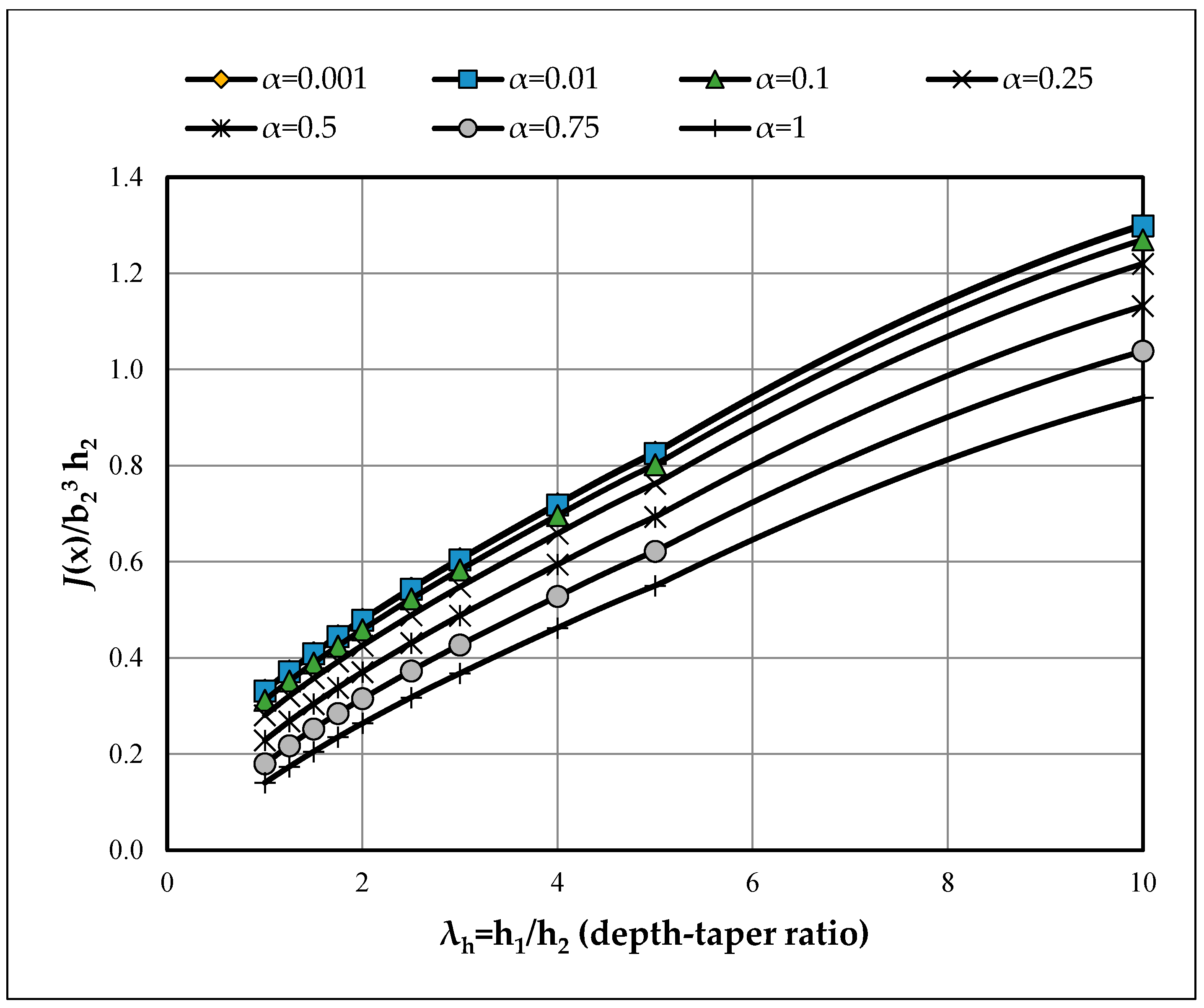
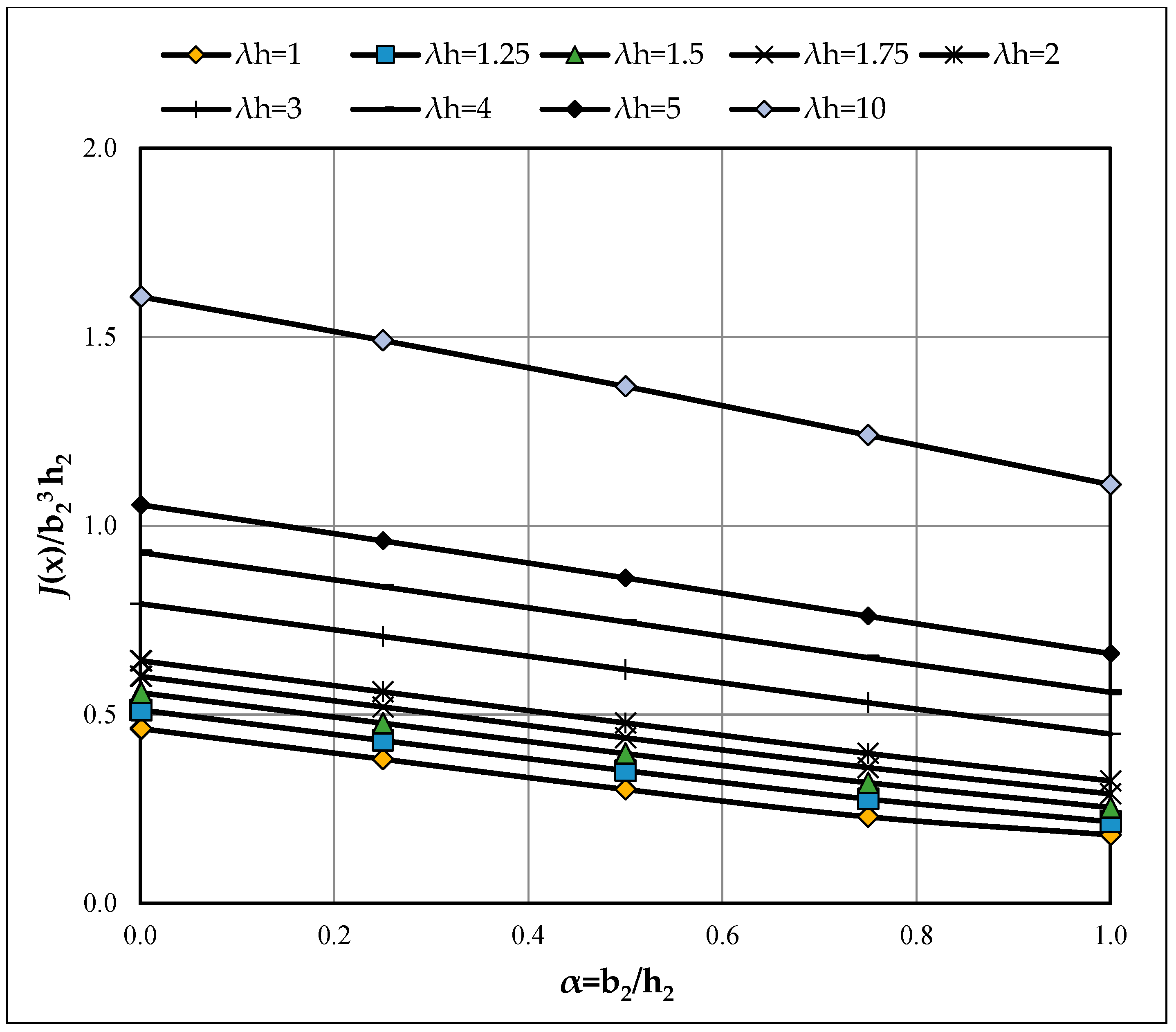
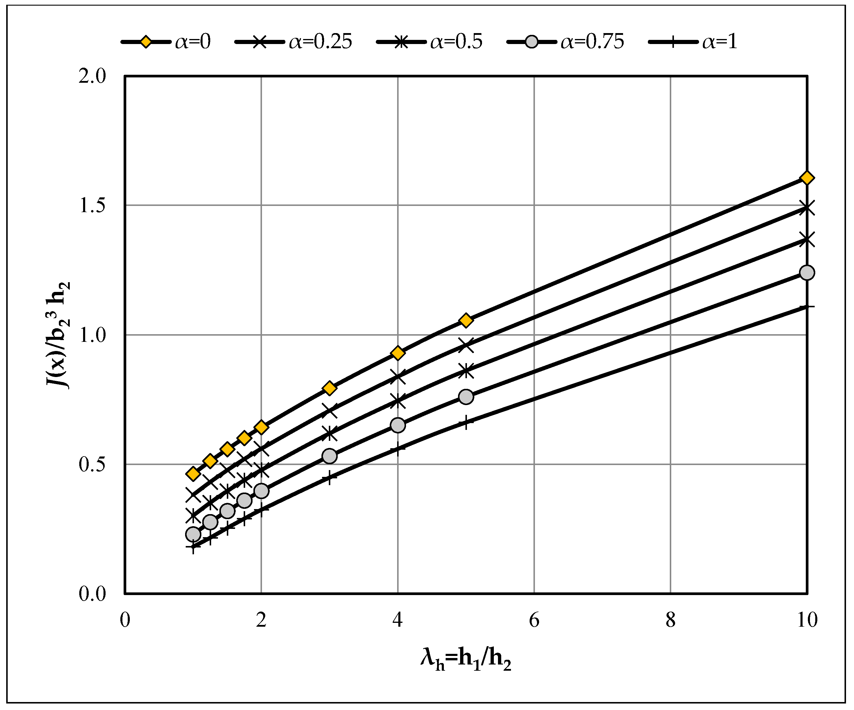
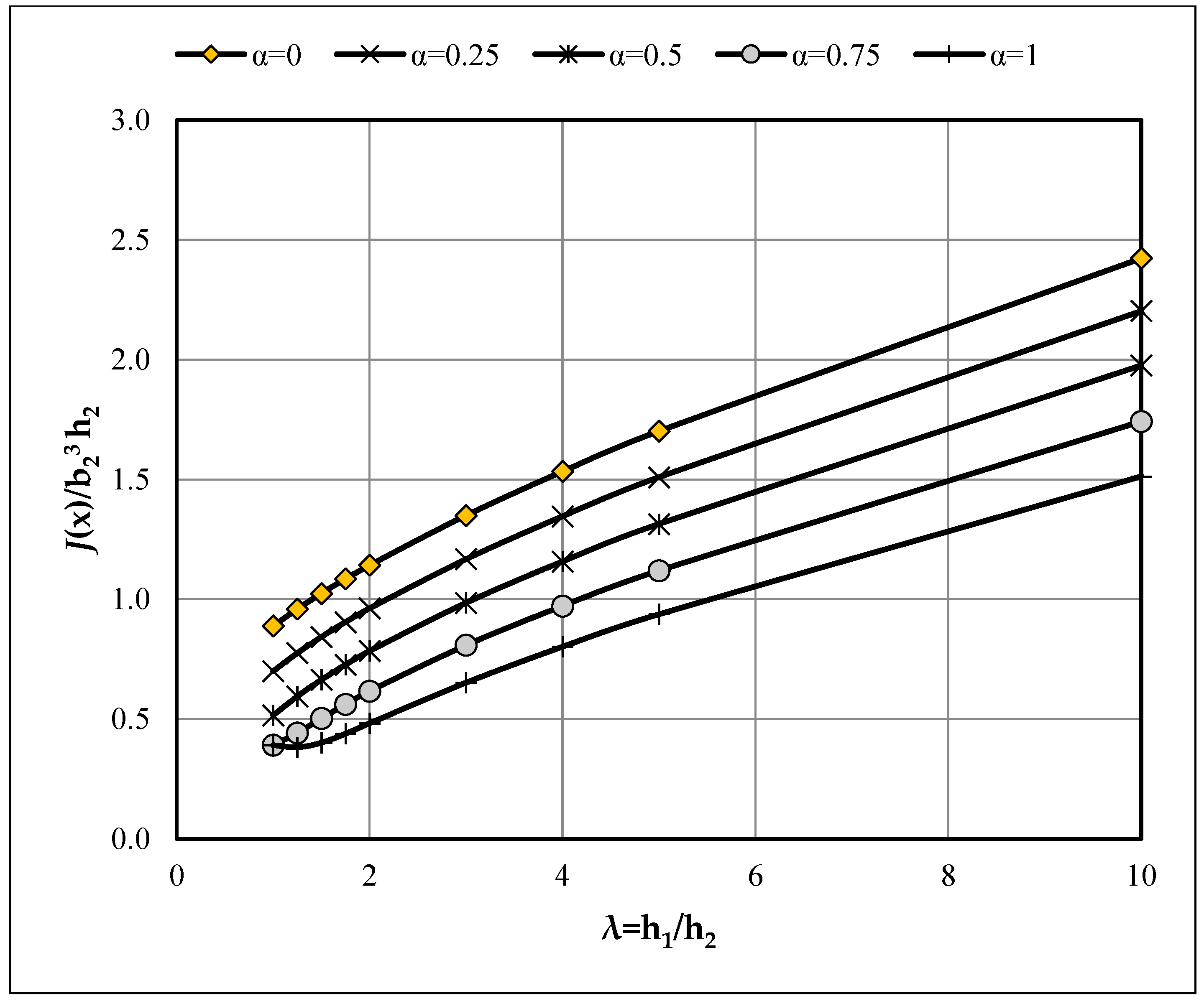
The effect of aspect ratio (α) is as follows: for fixed λ_h, I(x) increases with α, and therefore, f decreases. Narrower sections (smaller α) are torsionally stiffer in normalized terms. These trends are visible in Figure A1 (variation of I(x) with α at fixed λ_h)—which shows a smooth, monotone increase—and in Figure A3 (variation of f with λ_h at fixed α)—which shows an approximately linear increase of f with λ_h. For example, for α = 1.00 (singly tapered, λ_b = 1), f rises from 0.1408 at λ_h = 1 to 0.5504 at λ_h = 5, illustrating the amplification of normalized torsional rigidity with stronger depth taper.

3.3. Doubly Tapered Members (λ_b > 1)

When both depth and width taper, the same qualitative patterns persist, with an additional sensitivity to λ_b:

The effect of depth taper (λ_h) is as follows.: for fixed α and λ_b, I(x) decreases and f increases with λ_h. The effect of width taper (λ_b) is as follows: For fixed α and λ_h, I(x) decreases and f increases as λ_b grows.

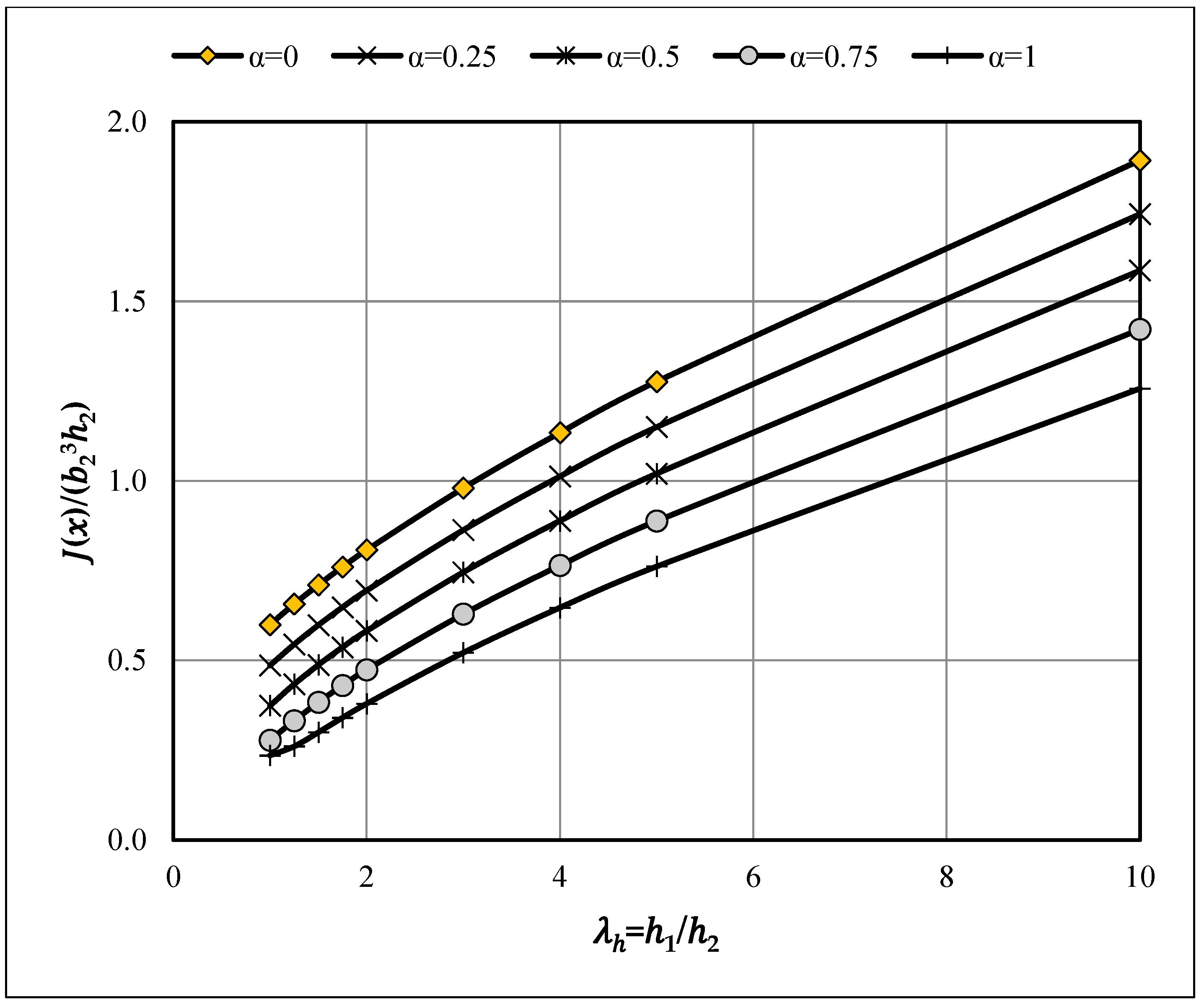
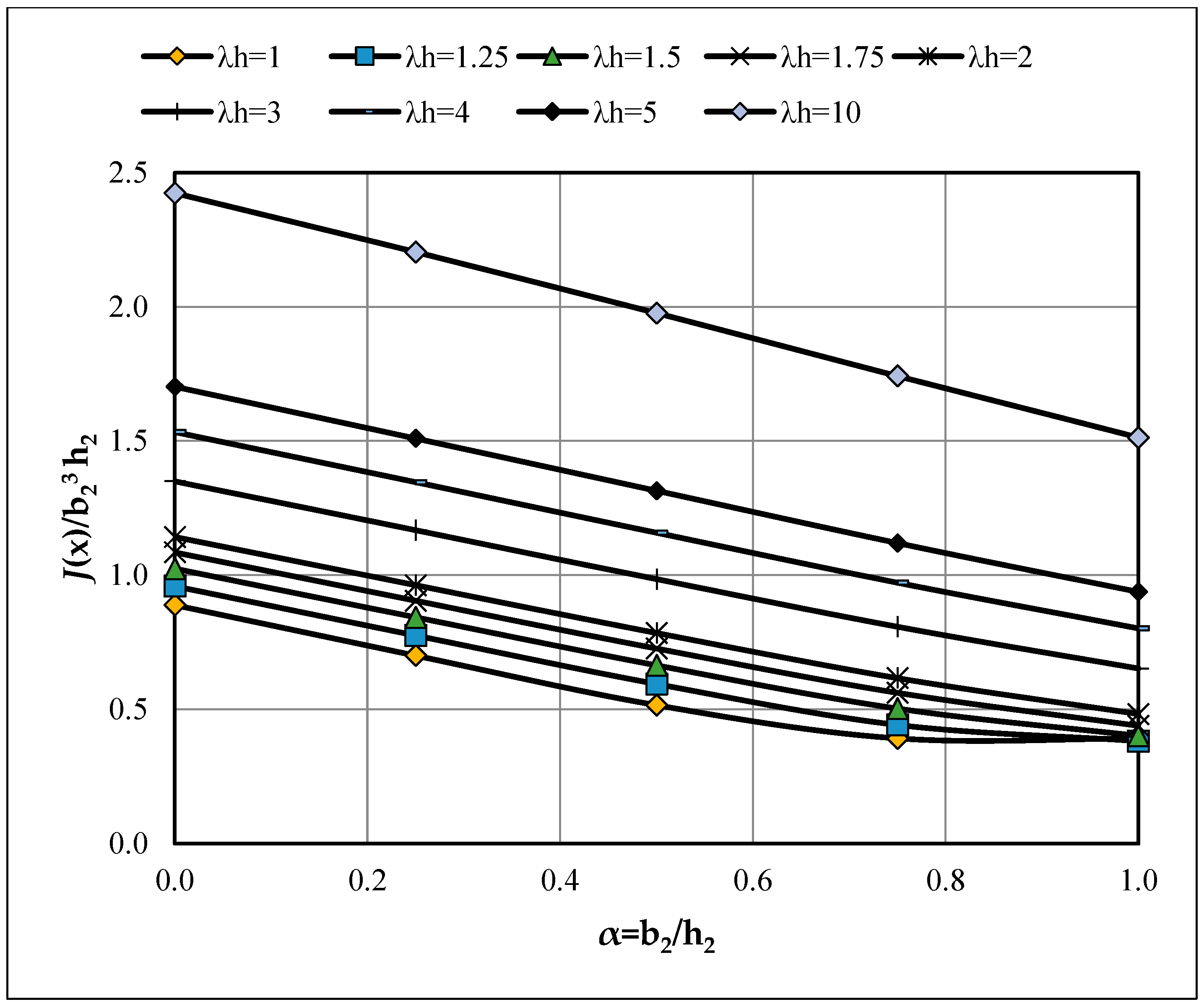
The effect of aspect ratio (α) is as follows: As in the singly tapered case, increasing α raises I(x) and lowers f. Representative curves in Figure A4, Figure A6 and Figure A8 (variation of f with α at fixed λ_b) show an approximately linear decrease of f with α, while Figure A5, Figure A7, Figure A9 and Figure A10 (variation with λ_h) show an approximately linear increase of f with λ_h. For compact design-oriented values, see the summary tables in the main text (e.g., Table 2), and consult Appendix A for the complete grids.

3.4. Limiting Behaviors, and Physical Interpretation

Very narrow sections (α → 0): I(x)→3 and f → 1/3 match the Saint-Venant solution for a prismatic rectangle. Accordingly, J = (b₂³h₂)/3 in this limit.

Very wide sections (α→ ∞): under the present normalization, I(x) → 0 and thus f → ∞; physically, GJ becomes very large and the twist θ = T/(GJ) tends to approach zero for a given torque T—i.e., very high torsional rigidity.

3.5. Interpretive Summary of Trends (Design Oriented)

An interpretive summary of trends is as follows: The numerical grids in Section 3 are accompanied by an interpretation that explains what the numbers mean and why the trends occur. In the prismatic, very-narrow rectangular limit, the dimensionless integral tends to I(x) → 3, so the normalized torsion coefficient satisfies f = J/(b₂³h₂) → 1/3, reproducing the classical rectangular result. Departing from this limit, the results reveal clear monotonicity with respect to geometry: at the fixed aspect ratio α = b₂/h₂, increasing depth-taper λ_h = h₁/h₂ raises f (i.e., increases normalized torsional rigidity), whereas at fixed λ_h, increasing α lowers f (narrower sections are torsionally stiffer than wider ones of the same h₂). For example, for α = 1.00 (singly tapered, λ_b = 1), f rises from 0.1408 at λ_h = 1 to 0.5504 at λ_h = 5; for a doubly tapered case with λ_h = 3 and α = 0.50, f increases from 0.8098 to 2.6522 as λ_h grows from 1 to 10. A mild non-monotonicity appears at α = 1.00 for λ_b = 3, where f dips at λ_h = 2 (0.7625 → 0.7154) before increasing at larger λ_h (up to 1.9284 at λ_h = 10); this reflects the competing influences of depth growth and width growth on the Saint-Venant torsion function. The design implication is as follows: since θ = T/(GJ), increases in f (and thus J) reduce twist under a given torque, while decreases in f elevate twist and shear flow—guiding proportioning during preliminary sizing and serviceability checks.

The validity of this equation is verified by the following examples:

Example 1 (Prismatic Bar):

Prismatic bar, h₁ = h₂ = 400 mm, λ = h₁/h₂ = 1.0, L = 4000 mm, T = 2.4 kN·m and G = 9281.37 MPa.

β = h₂/L = 400/4000 = 0.1

α = b₂/h₂ = 400/400 = 1.0

From Table A1, I(x) for these parameters is equal to (7)

$$J\left(x\right)={\displaystyle \frac{{b_2}^3{h}_2}{I_x}}=3.6056\times {10}^9{\mathrm{m}\mathrm{m}}^4$$

FEM solution:

This problem is solved by finite element method by using (STAAD Pro) software, the bar is subjected to constant torque at the free end (2.4 kN·m) max. shear stress obtained = τ_max = 0.122 MPa. And rotation (θ) = 2.7 × 10⁻⁴ rad, G$\theta$ = 2.506 MPa.

Analytical solution:

$${\left(G\theta \right)}_{analytic}={\displaystyle \frac{TL}{J\left(x\right)}}={\displaystyle \frac{TL\left[I\left(x\right)\right]}{{b_2}^3{h}_2}}=2.6625\mathrm{M}\mathrm{P}\mathrm{a}$$

$${\mathsf{\tau }}_{max}={\displaystyle \frac{{\pi }^3}{8}}\left(0.1\right){\displaystyle \frac{2.6625}{7.1}}=0.1453\mathrm{M}\mathrm{P}\mathrm{a}$$

$${\left(G\theta \right)}_{FEM}=2.506\mathrm{M}\mathrm{P}\mathrm{a}$$

Ratio of ${\left(G\theta \right)}_{analytic}/{\left(G\theta \right)}_{FEM}$ = 2.6625/2.506 = 1.0625.

Substituting G$\theta$ and I(x) into Equation (29), using G$\theta$ from analytical solution (2.6625 MPa), ${\mathsf{\tau }}_{max}=0.1453\mathrm{M}\mathrm{P}\mathrm{a}$.

Ratio of stress (R) ${\displaystyle \frac{{\mathsf{\tau }}_{max}Analytical}{{\mathsf{\tau }}_{max}FEM}}={\displaystyle \frac{0.1453}{0.122}}=1.191$.

Using G$\theta$ from FEM solution (2.506 MPa), τ_max = 0.1365 MPa, and R = 0.1365/0.122 = 1.119. The comparison of results is acceptable.

Example 2 (Tapered Bar):

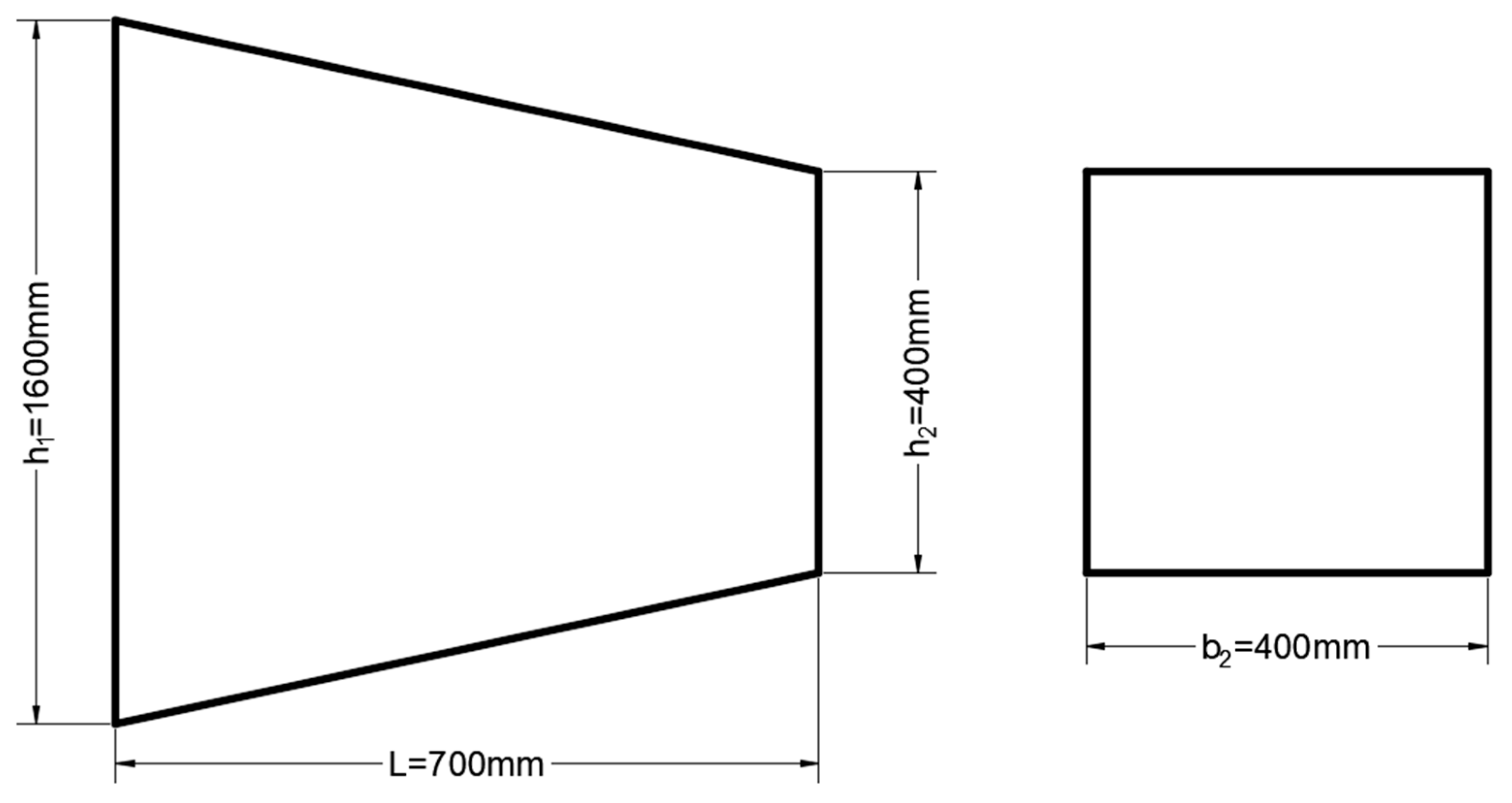
Tapered bar h₁ = 1600 mm, h₂ = 400 mm, b₂ = 400 mm, L = 700 mm, T = 2.4 kN·m and G = 9281.37 Mpa. As detailed in Figure 5:

$$\lambda ={\displaystyle \frac{h_1}{h_2}}=4.0$$

$$\alpha ={\displaystyle \frac{b_2}{h_2}}=1.0$$

$$\beta ={\displaystyle \frac{h_2}{L}}=0.57143$$

From Table A1; I(x) = 2.162216.

FEM solution

This problem is solved by finite element method by using (STAAD Pro) and gives the following results:

τ_max = 0.232 MPa, and rotation (θ) = 3.116 × 10⁻⁵ rad, G$\theta$ = 0.29 MPa.

Analytical solution:

$${\left(G\theta \right)}_{analytic}={\displaystyle \frac{TL}{J\left(x\right)}}={\displaystyle \frac{TLI\left(x\right)}{{b_2}^3{h}_2}}={\displaystyle \frac{0.4\times {10}^6\left(2.162216\right)700}{{400}^3\left(400\right)}}=0.1419\mathrm{M}\mathrm{P}\mathrm{a}$$

From Equation (29) and using G$\theta$= 0.1419 MPa,

$${\mathsf{\tau }}_{max}={\displaystyle \frac{{\pi }^3}{8}}\left(0.57143\right){\displaystyle \frac{0.1419}{2.162216}}=0.1453\mathrm{M}\mathrm{P}\mathrm{a}$$

$$StressratioR={\displaystyle \frac{0.1453}{0.232}}=0.626$$

Using G$\theta$= 0.29 MPa in Equation (29); ${\mathsf{\tau }}_{max}=0.297\mathrm{M}\mathrm{P}\mathrm{a}$,

$$StressratioR={\displaystyle \frac{0.297}{0.232}}=1.28$$

Using single Fourier series (equation), and taking a = b₂/2, b = h₂/2, and α = b₂/h₂, maximum shearing stress and torque are equal to

$${\tau }_{max}=G\theta {\displaystyle \frac{b_2}{\mathrm{L}}}[1-{\displaystyle \frac{8}{{\pi }^2}}\sum _{n=\mathrm{1,3},5}^{\mathrm{\infty }}{\displaystyle \frac{1}{n^{2}cosh\frac{n\pi }{2\alpha }}}]$$

$$T={\displaystyle \frac{G\theta }{L}}J$$

where

$$J={\displaystyle \frac{{\left(b_2\right)}^3\left(h_2\right)}{3}}[1-{\displaystyle \frac{192}{{\pi }^5}}\alpha \sum _{n=\mathrm{1,3},5}^{\mathrm{\infty }}{\displaystyle \frac{1}{n^5}}tanh{\displaystyle \frac{n\pi }{2a}}]$$

These equations are applied on the previous examples, one and two, and give the following results:

Taking n = 1 to 5, α = 1.0, β = 0.1

$$J={\displaystyle \frac{{\left(b_2\right)}^3\left(h_2\right)}{3}}[1-{\displaystyle \frac{192}{{\pi }^5}}1.0\left(0.9216\right)]=0.42178{\displaystyle \frac{{\left(b_2\right)}^3\left(h_2\right)}{3}}=0.1406{\left(b_2\right)}^3\left(h_2\right)$$

J = 3.6 × 109 mm⁴, which is very close to the value which is determined from Equation (9), (3.6056 × 109 mm⁴)

$${\tau }_{max}=\mathrm{G}\theta (0.1)[1-{\displaystyle \frac{8}{{\pi }^2}}\sum _{n=\mathrm{1,3},5}^{\mathrm{\infty }}{\displaystyle \frac{1}{n^{2}cosh\frac{n\pi }{2\alpha }}}]=0.0677G\theta$$

Using Gθ = 2.6625 MPa, τ_max = 0.18 MPa and stress ratio (R) = ${\displaystyle \frac{0.18}{0.122}}=1.447$.

Using Gθ = 2.506 MPa, τ_max = 0.17 MPa and stress ratio (R) = ${\displaystyle \frac{0.17}{0.122}}=1.39$.

4. Conclusions

This study derives a unified, design-oriented expression for the torsional constant J of non-prismatic rectangular bars with linearly varying geometry, encompassing both singly and doubly tapered configurations. By introducing the dimensionless integral I(x) and the geometric parameters (λ_h, λ_b, α) (depth taper, width taper, and aspect ratio), the formulation characterizes the spatial evolution of J along the span and elucidates its asymptotic behavior in the limits of very narrow and very wide sections. The expressions are specialized to prismatic and tapered cases and validated against membrane-analogy solutions (single- and double-Fourier series) and finite element analyses, showing close quantitative agreement. The principal conclusions are summarized below:

• This study derives a general expression for the torsional constant J of linearly tapered rectangular bars, covering the following: (i) singly tapered (non-prismatic) members with linearly varying depth and constant width, and (ii) doubly tapered members with both width and depth varying linearly along the member axis.
• In non-prismatic bars (singly tapered cross section), width of the cross section is constant and depth of the cross section is linearly changed along the axis of the bar.
• In non-prismatic bars (doubly tapered cross section), both width and depth of the cross section are linearly changed along the axis of the bar.
• For non-prismatic bars (singly tapered cross section), the value of the integral I(x) begins from value (3) for a very narrow cross section (small α) and exponentially decreased with increasing the tapered aspect ratio (λ), and parabolically increased with increasing the cross-section aspect ratio (α), while reversely, the value of torsion constant coefficient (f) begins from (1/3) and approximately linearly increased with increasing the tapered aspect ratio (λ) and linearly decreased with increasing the cross-section aspect ratio (α).

For a very narrow section α = 0.001, that is a very thin bar, I(x) = 3, and $J\left(x\right)={\displaystyle \frac{{b_2}^3{h}_2}{3}}$

• which is exactly equal to that determined by other references for rectangular sections.

For a very wide cross section α ≥ 10, I(x) reached zero, and J(x) reached infinity, then the angle of rotation $\theta ={\displaystyle \frac{TL}{GJ\left(x\right)}}$

• reached zero, that is, no torsional resistance of this cross-section type.
• For non-prismatic bars (doubly tapered cross section), the value of I(x) begins from (3) for a very narrow prismatic bar that is (λ_h = 1 and λ_b = 1) and (α) approximately zero, then the integral values decreased with increasing tapered depth ratio (λ_h) and increased with increasing aspect ratio of the cross section (α), which also decreased with increasing the tapered width ratio (λ_b). Reversely, the value of torsion constant coefficient J(x)/b₂³ h₂ begins from (1/3) for a very narrow prismatic bar that is (λ_h = 1 and λ_b = 1) and (α) approximately zero, then the values increased with increasing tapered depth ratio (λ_h) and decreased with increasing aspect ratio of the cross section (α), and also increased with increasing the tapered width ratio (λ_b).
• Analytical predictions for the torsional constant J and shear stress τ are evaluated for both prismatic (uniform) and tapered rectangular bars and benchmarked against membrane-analogy solutions (single- and double-Fourier series) and finite element (FE) analyses, demonstrating good agreement.

5. Design Use (Short Guide)

For reading charts/tables: Table A1, Table A2, Table A3, Table A4, Table A5, Table A6, Table A7, Table A8, Table A9, Table A10 and Table A11 give I(x); Table A12, Table A13, Table A14, Table A15, Table A16, Table A17, Table A18, Table A19 and Table A20 give J(x)/(b₂³h₂) = 1/I(x). Figure A1, Figure A2, Figure A3, Figure A4, Figure A5, Figure A6, Figure A7, Figure A8, Figure A9 and Figure A10 show trends vs. α = b₂/h₂, λ_h = b₁/h₂, λ_b = b₁/b₂. Fix the held parameter (from the title), pick your (α, λ_h) (and λ_b), and linearly interpolate if needed. Convert J(x) = b₂³h₂/I(x) or J(x) = (b₂³h₂) [J/(b₂³h₂)].

A quick workflow is as follows: Classify geometry: singly (λ_b = 1) or doubly tapered; compute α, λ_h, λ_b. Select the matching table/figure; read or interpolate the value. Compute J(x); then θ = T/(GJ) and check stresses per code. Verify against figure trends as a sanity check.

Limits of applicability include linear taper; solid rectangles; small strain, Saint-Venant torsion; uniform G; no material nonlinearity (cracking, plasticity, or therapy). Interpolate within bounds; avoid extrapolation (or confirm with FE).

References

1. Albegmprli, H.M.; Hashim, D.T.; Abbu, M.A. Combined behavior of reinforced concrete out-of-plane parts beams encased with steel section. Buildings 2025, 15, 2473. [Google Scholar] [CrossRef]
2. Cao, H.; Chen, D.; Zhang, Y.; Wang, H.; Chen, H. Finite element analysis of curved beam elements employing trigonometric displacement distribution patterns. Buildings 2023, 13, 2239. [Google Scholar] [CrossRef]
3. Darwin, D.; Dolan, C.W. Design of Concrete Structures, 16th ed.; McGraw-Hill Education: New York, NY, USA, 2021; 864p. [Google Scholar]
4. McCormac, J.C.; Brown, R.H. Design of Reinforced Concrete, 10th ed.; John Wiley & Sons, Inc.: Hoboken, NJ, USA, 2016; 650p. [Google Scholar]
5. Pincheira, J.A.; Montesions, G.J.P.; Wang, C.K.; Salmon, C. Reinforced Concrete Design, 9th ed.; Oxford University Press: Oxford, UK, 2018; 972p. [Google Scholar]
6. Wight, J.K.; MacGregor, J.G. Reinforced Concrete: Mechanics & Design, 5th ed.; Pearson: New York, NY, USA, 2009; 1128p. [Google Scholar]
7. Francu, J.; Nováčková, P.; Janíček, P. Torsion of a non-circular bar. Eng. Mech. 2012, 19, 45–60. [Google Scholar]
8. Campanile, A.; Mardarino, M.; Piscopo, V.; Pranzitelli, A. On the exact solution of non-uniform torsion for beams with axial symmetric cross-section. World Acad. Sci. Eng. Technol. 2009, 55, 36–45. [Google Scholar]
9. Saada, A.S. Elasticity: Theory and Applications, 2nd ed.; Krieger Publishing Company: Malabar, FL, USA, 1993; 775p. [Google Scholar]
10. Tso, W.K.; Ghobarah, A.A. Nonlinear non-uniform torsion of thin-walled beams. Int. J. Mech. Sci. 1971, 13, 1039–1047. [Google Scholar] [CrossRef]
11. Louis, A.M.; Danago, L.; Cabrera, R.M. Torsion of a rectangular prismatic bar: Solution using a power fit model. Philipp. Eng. J. 2007, 28, 77–98. [Google Scholar]
12. Nguyen, N.D.; Nguyen, T.K.; Vo, T.P.; Nguyen, L.B. Bending, buckling and free vibration behaviors of thin-walled functionally graded sandwich and composite channel-section beams. Mech. Based Des. Struct. Mach. 2023, 51, 932–960. [Google Scholar] [CrossRef]
13. Chaikittiratana, A.; Wattanasakulpong, N. Gram–Schmidt–Ritz method for dynamic response of FG-GPLRC beams under multiple moving loads. Mech. Based Des. Struct. Mach. 2022, 50, 2427–2448. [Google Scholar] [CrossRef]
14. Arda, M.; Aydoğdu, M. Vibration analysis of carbon nanotube mass sensors considering both inertia and stiffness of the detected mass. Mech. Based Des. Struct. Mach. 2022, 50, 841–857. [Google Scholar] [CrossRef]
15. Akgöz, B.; Civalek, Ö. Buckling analysis of functionally graded tapered microbeams via Rayleigh–Ritz method. Mathematics 2022, 10, 4429. [Google Scholar] [CrossRef]
16. Civalek, Ö.; Akbaş, Ş.D.; Akgöz, B.; Dastjerdi, S. Forced vibration analysis of composite beams reinforced by carbon nanotubes. Nanomaterials 2021, 11, 571. [Google Scholar] [CrossRef] [PubMed]
17. Gere, J.M. Mechanics of Materials, 5th ed.; Brooks/Cole, Thomson Learning: Boston, MA, USA, 2001. [Google Scholar]
18. Timoshenko, S.P.; Gere, J.M. Theory of Elastic Stability; Courier Corporation: North Chelmsford, MA, USA, 2012. [Google Scholar]
19. Boresi, A.P.; Schmidt, R.J. Advanced Mechanics of Materials, 6th ed.; John Wiley & Sons, Inc.: Hoboken, NJ, USA, 2003; 695p. [Google Scholar]
20. Timoshenko, S.; Goodier, J.N. Theory of Elasticity; McGraw-Hill Book Company, Inc.: New York, NY, USA, 1951; 506p. [Google Scholar]
21. Barber, J.R.; Klarbring, A. (Eds.) Solid Mechanics and Its Applications; Springer: Berlin/Heidelberg, Germany, 2003; Volume 107, 410p. [Google Scholar]
22. Ameen, M. Computational Elasticity, Rev. ed.; Alpha Science International Ltd.: Oxford, UK, 2008; 509p. [Google Scholar]
23. Sadd, M.H. Elasticity: Theory, Applications, and Numerics, 2nd ed.; Academic Press: Cambridge, MA, USA; Elsevier Inc.: New York, NY, USA, 2009; 536p. [Google Scholar]
Figure 1. Bar with continuously varying cross section and constant torque.
Buildings 15 03926 g001
Figure 2. Non-prismatic singly tapered cross section.
Buildings 15 03926 g002
Figure 3. Non-prismatic doubly tapered cross section.
Buildings 15 03926 g003
Figure 4. Membrane Cross Section and Corresponding Equilibrium under Distributed Load.
Buildings 15 03926 g004
Figure 5. Membrane cross section and membrane equilibrium.
Buildings 15 03926 g005