A Multi-Stage Framework Combining Experimental Testing, Numerical Calibration, and AI Surrogates for Composite Panel Characterization

Abstract

Composite modular panels are increasingly used in modern buildings, yet their layered behavior makes mechanical characterization and modeling difficult. This study presents a novel hybrid framework that integrates analytical, numerical, and AI-driven approaches for the mechanical characterization of composite panels. The system combines a layered concrete configuration with embedded steel reinforcement, and its performance was evaluated through experimental testing, analytical formulation, finite element simulations, and artificial intelligence techniques. Full-scale bending and shear tests were conducted and results in terms of displacements were compared with in silico simulations. The equivalent elastic modulus and thickness were suggested via a closed-form analytical procedure and validated numerically, showing less than 3% deviation from experiments. These equivalent parameters were used to simulate the dynamic response of a two-storey prototype building under harmonic excitation, with simulated modal periods differing by less than 10% from experimental data. To generalize the method, a parametric dataset of 218 panel configurations was generated by varying material and geometric properties. Machine learning models including Artificial Neural Network, Random Forest, Gradient Boosting, and Extra Trees were trained on this dataset, achieving R² > 0.98 for both targets. A graphical user interface was developed to integrate the trained models into an engineering tool for fast prediction of equivalent properties. The proposed methodology provides a unified and computationally efficient approach that combines physical accuracy with practical usability, enabling rapid design and optimization of composite panel structures.

1. Introduction

The accurate identification of structural dynamics is a fundamental aspect of structural engineering, particularly for performance evaluation, seismic assessment, and health monitoring of both traditional and novel systems. Over the past few decades, there has been a growing need for lightweight, prefabricated, and high-efficiency building components. This has led to the use of sophisticated composite panels in modular construction. These systems often exhibit complex mechanical behavior because of their layered composition and interactions between different materials and reinforcements. As such, characterizing their equivalent mechanical properties becomes essential for integrating them into large-scale structural models and for developing practical design tools that reflect their true behavior under loading. Dynamic identification of a structure refers to the set of analytical, experimental, and data-driven techniques used to determine its dynamic properties, such as natural frequencies, vibration modes, and damping ratios. These parameters are critical for evaluating structural performance under operational or extreme loading conditions [1,2].

Experimental modal analysis, often referred to as an “inverse problem,” involves deducing structural properties from measured dynamic responses, in contrast to direct problems where the response is calculated from known properties and inputs. Initially developed for aerospace applications, this method has since found broad use in automation, robotics, and civil infrastructure. Extensions to the elastic-plastic domain have included shear-layer behavior [3], shakedown and limit-load analysis [4], and lower-bound solutions for complex geometries [5]. In civil engineering, dynamic tests are frequently performed both as part of the design verification phase and for condition assessment of aging or post-seismic structures. Among the most common procedures is the application of sinusoidal excitation at varying frequencies to extract modal parameters experimentally, which are then used to calibrate finite element (FE) models [6,7,8].

Modern composite panels pose a challenge in dynamic assessment because of their multi-layered structure and interactions between core, reinforcement, and external loads [9,10]. Early experimental modal studies have focused on fundamental dynamics of such elements. For instance, Bocheński et al. [11] performed modal analysis of composite box-beams and verified mode shapes and natural frequencies experimentally before comparing with numerical models. Similarly, research on fiber-reinforced and sandwich panels has confirmed that targeted modal identification effectively captures equivalent stiffness properties under dynamic loading [12,13]. While these works establish basic identification strategies, they often lack a systematic approach specifically for modular, prefabricated panel systems.

Homogenization and inversion techniques, based on combining experimental data with FE modeling, have emerged as effective means to derive equivalent panel parameters for dynamical analyses. Rainieri et al. [14,15] applied inverse dynamics procedures to infer equivalent elasticity and shear properties, supporting FE calibration. Esposito et al. [16] proposed an automated FEM procedure for the identification of crack propagation in both homogeneous and heterogeneous media. However, this inversion requires repeated model updating, which becomes computationally expensive when studying multiple configurations-such as variable reinforcement layouts, core moduli, and loading situations. This challenge is especially relevant in prefabricated construction, where designers need to explore a wide design space efficiently.

To address this, surrogate modeling and machine learning (ML) approaches have gained traction in structural engineering. Arndt et al. [17] developed a reduced-dimension surrogate that integrates FE simulations and experimental tests for composite/metal structures. Sheini Dashtgoli et al. [18] used GRNN models to predict the load–displacement behavior of bio-based sandwich panels with high accuracy (${\mathrm{R}}^2> 0.99$), based on geometry and material inputs. Viotti and Gomes [19] proposed a ML framework for delamination detection in sandwich composites using modal data from FE simulations. Their models, combining classification and regression, achieved near 85% accuracy in localizing damage, highlighting the potential of ML for SHM tasks in layered structures. Kamarian et al. [20] applied shallow and deep neural networks to predict the bending behavior of sandwich beams with 3D-printed auxetic cores and natural fiber composite face sheets. Their models accurately estimated specific energy absorption and load-deflection curves, confirming the suitability of ML for capturing nonlinear mechanical responses in sustainable composite systems. Mottaghian and Taheri [21] combined FE cohesive zone modeling with ML to predict the axial impact response of adhesively bonded joints using sandwich composite adherends. By training neural networks and genetic models, they accurately estimated load-bearing capacities and derived cost-effective empirical design formulas, demonstrating the efficiency of hybrid FE–ML approaches in joint performance prediction. Vaishali et al. [22] developed a Gaussian process ML model to enhance vibration analysis of composite and sandwich plates for large-scale simulations. Khan et al. [23] provided a comprehensive review of ML-based damage assessment in smart composite structures. They stressed how important it is to use discriminative features and matching ML algorithms for accurate detection, localization, and quantification of various failure modes such as delamination, matrix cracking, and fiber breakage. Ribeiro Junior and Gomes [24] provided a comprehensive review of ML techniques for damage assessment in composite structures and emphasized the growing reliance on neural networks for detecting and quantifying damage.

Despite the promise of these methods, their application remains fragmented across different structural systems. Some focus on damage detection in plates or beams, others on micro-scale composite micromechanics. Few studies combine a validated inversion-based equivalent model with a fast ML surrogate that is practically deployed on a user interface. In particular, no existing work to our knowledge offers a complete framework for composite panels that includes (i) experimental modal testing, (ii) FE model inversion, (iii) ML surrogate prediction, and (iv) a user-accessible GUI.

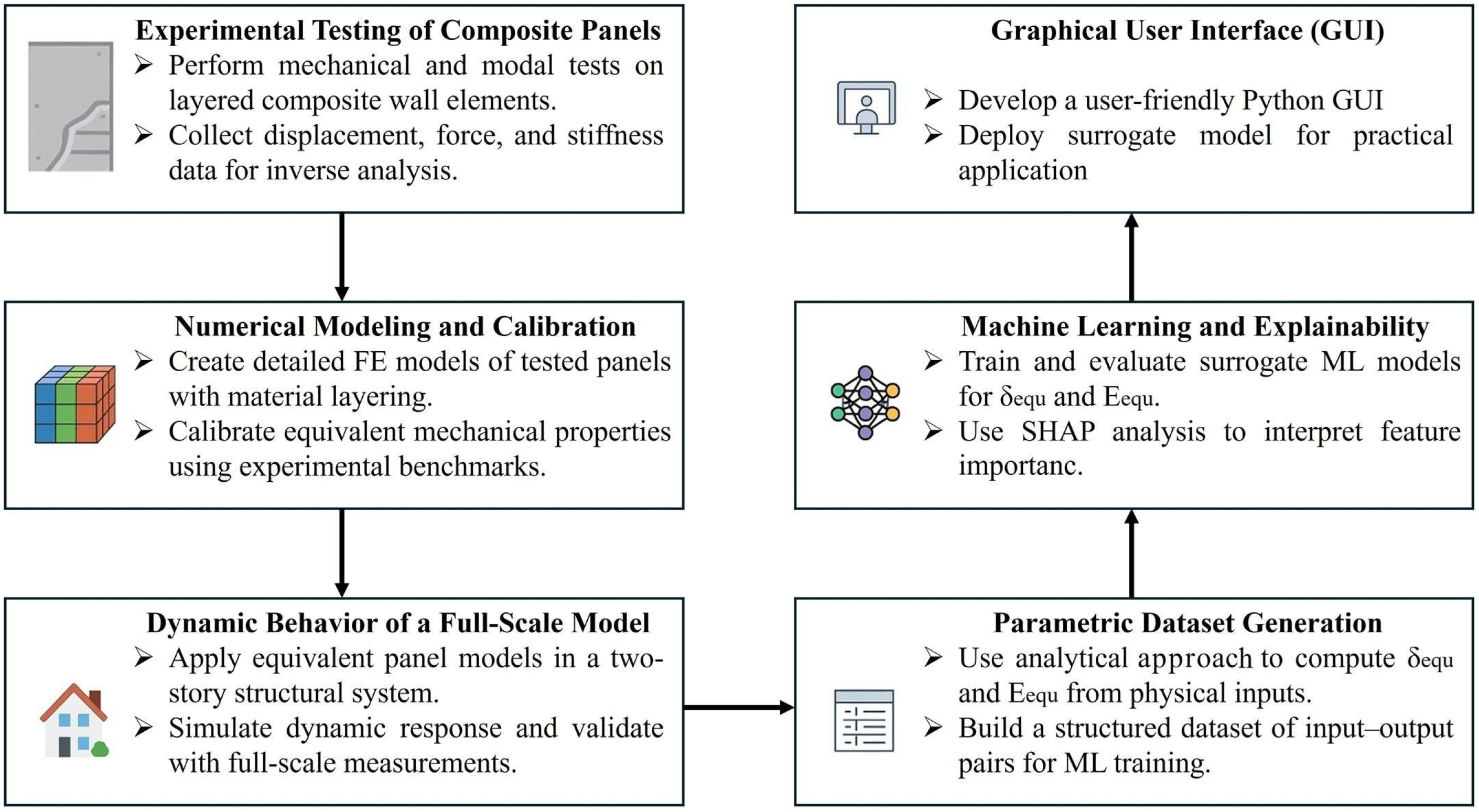
In this framework, the present work investigates the dynamic and static behaviour of an innovative composite panel system through a multi-step workflow that combines laboratory testing, numerical simulation, and ML techniques. The panel has been subjected to experimental testing, and a FE model has been calibrated using the measured modal response. An equivalent homogeneous panel has then been derived and used to simulate the dynamic behaviour of a two-story frame structure subjected to vibrodyne excitation [25,26,27]. Comparison between experimental and numerical results confirmed the consistency of the equivalent model and validated its use for further parametric analysis. Furthermore, the present study integrates a data-driven methodology to complement the experimental and numerical framework. While the analytical formulation remains the foundation for deriving equivalent panel properties, its repeated application across different configurations can become time-consuming and computationally inefficient, especially during early-stage design or optimization. To address this limitation, we introduce a ML-based surrogate modelling strategy aimed at predicting two key equivalent parameters including the equivalent elastic modulus and the equivalent panel thickness directly from the composite layout and load conditions. This surrogate approach enables rapid prediction of the global structural response without relying on full FE simulations or iterative inversion. Four different ML algorithms including artificial neural networks (ANNs), random forest (RF), XGBoost (XGB), and Extra Trees were trained and validated using a parametric dataset derived from the inversion process, and their performance was assessed using cross-validation and standard evaluation metrics. The proposed tool does not replace the theoretical framework but rather extends it by offering a lightweight, accurate, and practical predictive solution. To enhance engineering usability, a user-friendly web-based GUI was developed using the Streamlit platform. This allows structural designers to enter panel specifications and get expected values in engineering units. This capability is quite helpful for sensitivity analysis and early design validation.

Contributions and Novelty of the Study

This work proposes a hybrid analytical–numerical–data-driven framework for the mechanical characterization and surrogate modeling of prefabricated composite panels. The main contributions and novelties can be summarized as follows:

• Integrated experimental–numerical–AI workflow: The study combines full-scale experimental testing, finite element calibration, analytical homogenization, and machine learning surrogate modeling within a single, reproducible framework.
• Closed-form homogenization formulation: A simplified analytical model is derived to compute the equivalent elastic modulus and thickness of layered concrete panels under combined bending and shear, validated against experiments and 3D FE simulations.
• Dynamic validation on a full-scale structure: The equivalent model is applied to simulate and replicate the dynamic behavior of a two-storey prototype building under vibrodyne excitation, confirming its predictive reliability.
• Surrogate modeling for design generalization: A machine learning surrogate trained on 218 parametric FE–analytical cases enables instant prediction of equivalent stiffness parameters from geometric and material inputs, reducing computational cost by several orders of magnitude.
• Deployment through an engineering-ready GUI: A user-accessible Streamlit interface translates the analytical–ML framework into a practical tool for engineers, allowing rapid prediction and data export without programming effort.

Together, these aspects establish a novel, end-to-end methodology that bridges physical testing, analytical formulation, numerical simulation, and AI-based design assistance; a combination not previously reported for modular composite panel systems.

2. Experimental Characterization of Composite Panels

2.1. Panel Geometry and Materials

The structural element investigated is a prefabricated, multi-layered composite panel designed for modular and seismic-resistant buildings. The panel has overall dimensions of 2000 mm (H) × 1500 mm (L) × 320 mm (t). Its architecture follows a sandwich-type configuration of three concrete layers with distinct roles, enclosed by a welded 10 mm steel frame and reinforced with B450C rebars.

Sandwich Layer Configuration

The top and bottom layers (each 130 mm thick) are made of lightweight concrete with polystyrene beads, reducing mass and improving thermal insulation. The 60 mm high-strength concrete (C35/45) core provides the main flexural and shear contribution. This trilayer layout optimizes stiffness-to-weight ratio and ensures effective composite action through continuous casting without slip at interfaces.

The adopted thickness ratio (130 mm–60 mm–130 mm) was selected from sandwich panel mechanics and verified numerically. With a fixed total thickness of 320 mm and the measured moduli (lightweight layers E ≈ 21 GPa; core E ≈ 36 GPa), a parametric check based on u = u_b + u_s (first-order shear deformation) and 3D FE models showed that: (i) faces control EI and bending stiffness, (ii) the core governs shear stiffness GA, and (iii) the optimal range for the core is ≈60–70 mm if the shear share of total deflection is kept within ≈20–25% at service load. A thinner core increased u_s; a thicker core produced marginal bending gains but higher mass and longer vibration periods. The 60 mm core also minimizes areal mass because the core concrete is the densest layer, while still matching the experimental mid-span displacement (1.56 mm at 50 t). The 130 mm faces provide sufficient stiffness, local bearing capacity at supports, and rebar cover/anchorage for Φ16 bars within the steel frame.

2.2. Steel Frame and Reinforcement

The entire panel is confined within a 10 mm thick rectangular steel frame ($\delta f$), welded along its edges. This frame ensures confinement, distributes concentrated loads, and simplifies connection to surrounding structural elements. In addition, the panel incorporates an internal steel reinforcement system using B450C steel bars:

• Five vertical bars ($\mathsf{\Phi }$16 mm), spaced 400 mm apart ($i_L$), are embedded along the height of the panel.
• Three horizontal bars ($\mathsf{\Phi }$16 mm), spaced 375 mm apart ($i_D$), are embedded along the panel width.

The reinforcement layout, as detailed in Figure 1, ensures sufficient ductility and crack control under both flexural and in-plane loading scenarios. It also contributes to panel integrity during handling and installation.

Material Properties

The mechanical properties of all materials used in the panel are summarized in

Table 1. Concrete mechanical properties.

	${\mathit{f}}_{\mathit{c}\mathit{k}}$ [MPa]	$\mathit{E}$ [MPa]	$\mathit{\nu }$
Top Layer	20	21,000	0.24
Middle Layer	35	36,000	0.30
Bottom Layer	20	21,000	0.24

and

Table 2. Steel rebars mechanical properties.

${\mathit{f}}_{\mathit{y}}$ [MPa]	$\mathit{E}$ [MPa]	$\mathit{\nu }$
450	210,000	0.30

.

These include:

• Concrete: Characteristic compressive strength ($f_{ck}$), elastic modulus ($E$), and Poisson’s ratio ($\mathsf{\nu }$) for both lightweight and structural concrete layers.
• Steel: Yield strength ($f_y$), elastic modulus, and Poisson’s ratio for both the perimeter frame and the embedded rebars. All materials were sourced from certified suppliers and comply with European standards for structural and prefabricated concrete components.

2.3. Experimental Setup and Instrumentation

To characterize the mechanical performance of the composite panel under realistic service conditions, a dedicated full-scale experimental campaign was conducted. The primary objective of the setup was to analyze both bending and shear behavior through controlled loading schemes while accurately measuring the resulting displacements and deformation patterns.

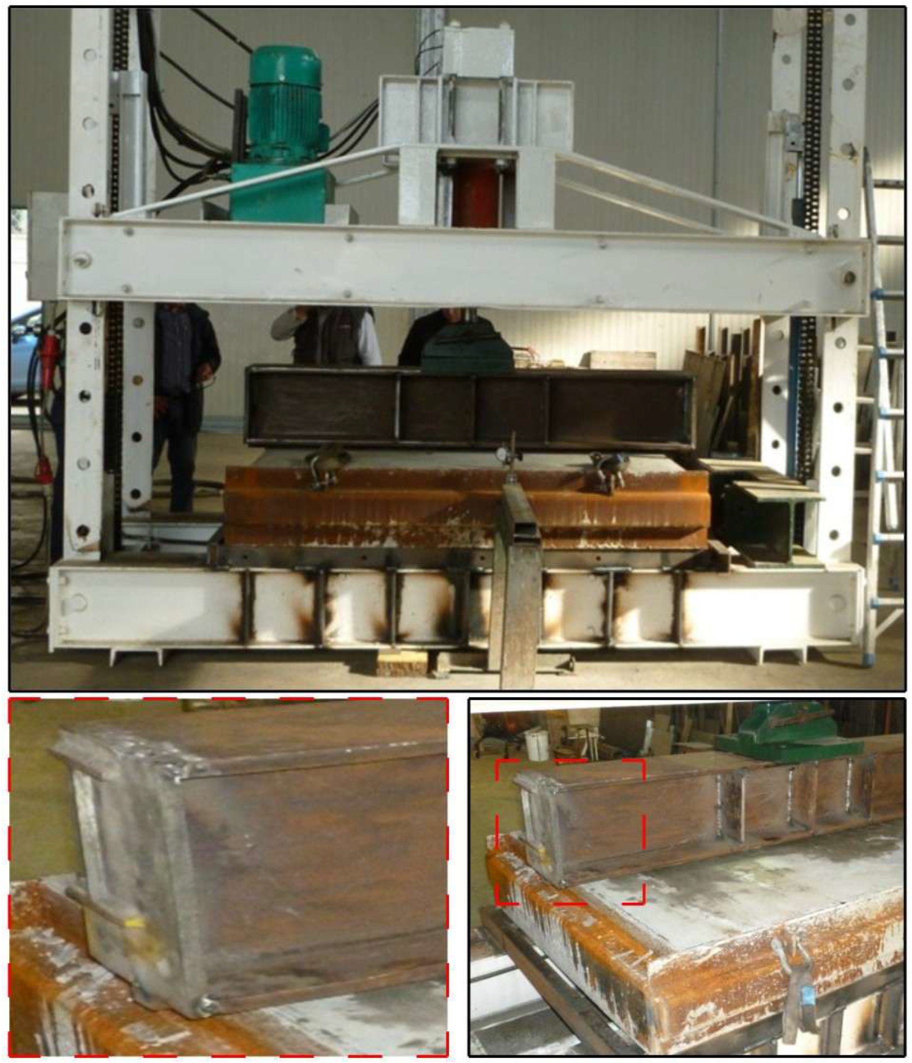
The experimental framework was designed to simulate the panel’s in situ boundary conditions. Specifically, the panel was vertically positioned between two rigid slabs and loaded orthogonally through a centrally applied force, thereby replicating the actual configuration of infill panels constrained between the floor and ceiling of a multistory building. The vertical loading was applied using a hydraulic actuator fixed to the upper crossbeam of a steel reaction frame. The actuator imposed a monotonic load at the mid-height of the panel, corresponding to the centroid of the core concrete layer.

To monitor the structural response, a precise instrumentation system was deployed. Three analog displacement transducers (LVDTs) were employed to capture the out-of-plane displacements:

• LVDT-1 and LVDT-2 were mounted symmetrically at the left and right support points, aligned along the panel’s mid-span. These sensors recorded the vertical movements at the supports, enabling the estimation of rigid-body displacement components due to boundary compliance or localized rotations.
• LVDT-3 was positioned at the geometric center of the panel, aligned with the loading point. This transducer measured the central deflection and served as the primary indicator of the panel’s flexural response.

All sensors were connected to a high-resolution data acquisition system that synchronized displacement and load readings throughout the test. The instrumentation layout ensured the separation of rigid and elastic displacements by enabling differential analysis of the LVDT readings. This distinction was critical for accurately computing the true elastic deformation of the structure.

The loading procedure followed an incremental protocol, initially applying loads in 1-ton steps up to 60 tons (600 kN). Beyond this threshold, the increment was increased to 2 tons per step, reaching a maximum load of 100 tons. This conservative escalation was selected to prevent damage to the testing equipment while still capturing the panel’s non-linear and post-yield behavior.

A detailed schematic of the experimental setup, including support conditions, actuator position, and transducer placements, is presented in Figure 2. The overall configuration ensured repeatable boundary conditions, minimized geometric uncertainties, and supported high-fidelity interpretation of the bending and shear response.

The loading rate during all tests was maintained at approximately 10 kN/min to ensure quasi-static conditions and avoid dynamic effects. The applied load was increased stepwise under force control using a calibrated hydraulic actuator. Displacement control was performed through analog dial gauges (resolution 0.01 mm) connected to a synchronized acquisition system. Readings were taken at each 10 kN load increment, corresponding to approximately one-minute intervals, allowing accurate monitoring of the load–displacement relationship and time-dependent response.

2.4. Test Procedure and Key Observations

The campaign included independent bending and shear tests. Each configuration was tested on one full-scale specimen due to cost and setup constraints, with repeatability verified through load–unload cycles. The limited number of tests was compensated by calibrated analytical and numerical models. The strong consistency between experimental and simulated results supports the reliability of the adopted methodology.

2.5. Bending Test

The bending test was performed using a three-point loading configuration, in which the panel was horizontally supported at both ends and subjected to a concentrated vertical load at mid-span. The steel frame housing the panel was fixed to two reaction supports, simulating hinged boundary conditions typically encountered in structural infill applications.

The hinged boundary conditions were physically achieved by placing the panel on two welded double-T steel supports integrated into the testing frame. These supports allowed free rotation at the panel edges while restraining vertical translation, thereby reproducing a simply supported condition. The applied load was transmitted through a stiff steel beam designed to distribute the force uniformly along the panel width. To obtain a narrow and well-defined contact area, a rectangular steel bar with a 2 cm contact width was welded beneath the loading beam, ensuring an almost line-type contact and accurate simulation of a uniform bending load. This configuration guaranteed repeatable and well-controlled boundary conditions throughout the test series.

The loading piston was mounted vertically at the panel’s geometric center, directly above the core layer. The load was applied incrementally in a quasi-static fashion, starting from an initial preload and increasing in 1-ton steps up to 60 tons. This range corresponds to the expected service loading and the onset of nonlinear deformation. For safety and to ensure mechanical stability, the increment was then increased to 2 tons up to a maximum applied load of 100 tons (approximately 1 MN), which approached the operational limits of the testing system without compromising the integrity of the specimen.

At each load step, the vertical displacements were recorded using the three LVDTs. To isolate the elastic deflection of the panel, the average displacement of the support transducers (LVDT-1 and LVDT-2) was subtracted from the central transducer (LVDT-3). This correction removed the contribution of rigid-body movements caused by settlement or compliance of the supports.

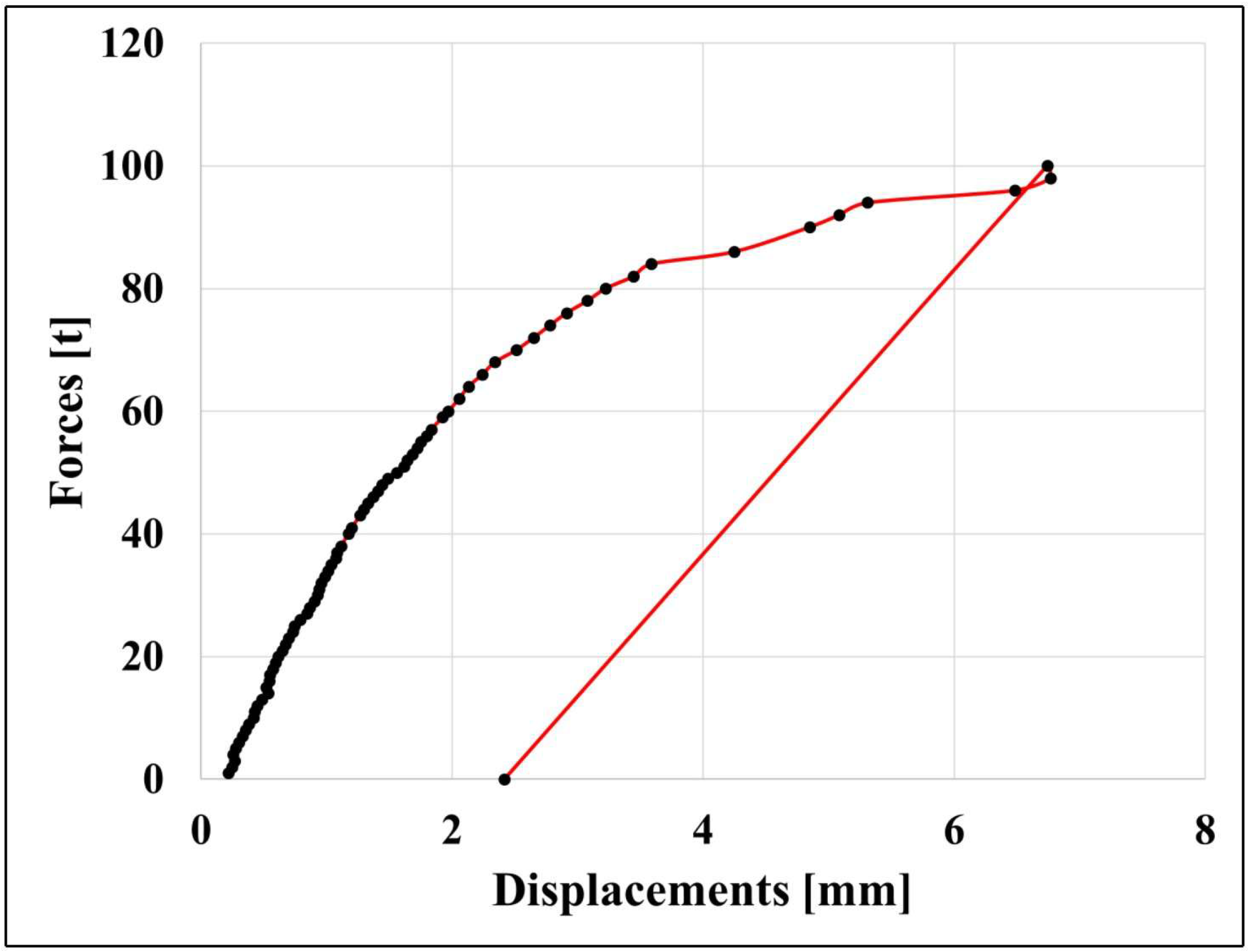
The resulting load–displacement curve (Figure 3) showed an initially linear elastic response up to approximately 48–55 tons, followed by a clear deviation from linearity indicative of material nonlinearity and progressive plasticization. Three load steps (39, 42, and 58 tons) showed minor anomalies in displacement behavior, likely due to localized slippage or temporary sensor noise, and were conservatively excluded from the elastic regression analysis. A linear regression was applied to the initial elastic portion of the load–deflection curve. The angle of the elastic branch ($\mathsf{\alpha }$) was calculated by evaluating the tangent of the slope of consecutive segments. The final estimate of $\mathsf{\alpha }= 1.545$ radians corresponds to a slope of approximately 38.70 in the force–displacement diagram, confirming the panel’s high stiffness in the pre-yield regime. Physically, this angle represents the inclination of the elastic branch in the load–displacement curve, where a larger α denotes a stiffer response. Its tangent (tan α ≈ 38.7) expresses the bending stiffness directly as the slope of the elastic region, linking graphical representation and mechanical behavior. This value was consistent with analytical expectations based on layered composite behavior.

Two full-scale bending tests were conducted, and both exhibited almost identical elastic stiffness and ultimate strength. The maximum load recorded was 100 t, corresponding to central displacements of 6.4 mm and 6.2 mm in the first and second tests, respectively. Due to the high consistency between the two datasets, only one representative load–displacement curve is reported in Figure 3.

2.6. Shear Test

The in-plane shear behavior was evaluated through a cantilever test configuration. To reproduce a clamped boundary condition, the panel was welded along one vertical edge to the testing frame at both the top and bottom ends. This arrangement prevented any rotation or translation of the restrained edge, ensuring full fixity. The opposite vertical edge was left free, and the horizontal load was applied at its upper end to induce in-plane shear deformation. This configuration established a clear fixed–free boundary condition, providing controlled load transfer and accurate measurement of the panel’s shear response. The panel was fixed vertically at its base and loaded horizontally at its top edge, replicating the lateral forces typically induced by seismic or wind loads in building applications. A single-point horizontal force was applied using a servo-controlled actuator connected to a steel load distribution plate (Figure 4a,b). To measure the shear deformation, three high-precision comparators were mounted at strategic locations along the vertical axis. These instruments captured both elastic displacement and rigid-body rotation of the panel. The measurements enabled the separation of shear strain from global lateral translation.

The resulting load–displacement curve (Figure 4c) exhibited an initially linear progression, followed by a gradual transition to non-linear behavior. The stiffness and deformation capacity observed in this test confirmed the structural contribution of the steel frame and the integrity of the sandwich configuration under lateral loading. Quantitatively, the panel displayed an almost entirely linear elastic response up to the maximum applied horizontal load of about 90 kN, without any visible cracking or localized yielding. The measured horizontal stiffness was approximately 13.8 kN/mm, corresponding to an average engineering shear strain of ≈0.0005 at the maximum displacement. The associated shear stress along the loaded edge was about 0.43 MPa, which remains below the expected cracking threshold of the lightweight concrete layers (≈0.9–1.0 MPa). These results indicate that the specimen behaved elastically throughout the test, consistent with theoretical stiffness predictions derived from the homogenized analytical model.

Key Observations:

• The panel exhibited robust structural behavior under both bending and shear loads, with well-defined elastic regions and controlled post-yield deformation.
• The steel frame and internal reinforcement effectively limited excessive cracking and ensured ductility, even beyond the elastic threshold.
• The multi-layer composite design provided a favorable combination of stiffness, energy dissipation, and lightweight performance, confirming its suitability for modular structural applications.

These experimental results formed the basis for calibrating the numerical models and extracting homogenized equivalent properties, as discussed in the subsequent section.

In total, four full-scale composite panel specimens (1.50 × 2.00 m) were produced and tested: two under three-point bending and two under in-plane shear. The bending tests yielded consistent and overlapping load–displacement curves, confirming the stability of the setup and the reproducibility of results. Among the shear specimens, only one test was successfully completed, as the second experienced a setup malfunction during loading, which prevented reliable data acquisition. The results from the successful shear test were therefore used for model calibration and validation. Despite this limitation, the consistent bending tests and the high-quality shear data provided a sufficient experimental basis for model development and verification.

3. Numerical Modelling and Calibration

3.1. Finite Element Model Description

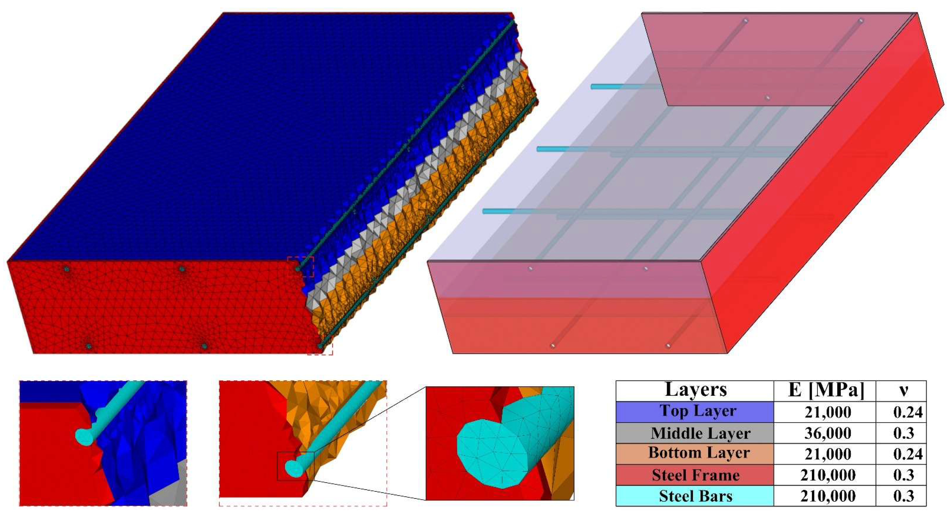
A detailed FE model was developed to simulate the mechanical behavior of the multi-layered composite panel under both bending and in-plane shear loads. The modeling was carried out using ANSYS Multiphysics environment (Ansys, Inc., Canonsburg, PA, USA) via the Ansys Parametric Design Language (ADPL), employing the 10-node tetrahedral SOLID187 (three degrees of freedom per node and quadratic shape functions) element type for all the panel’s constituents to ensure both computational efficiency and accurate strain distribution.

The geometry of the FE model precisely replicated the panel tested in the experimental campaign: 2000 mm height (H), 1500 mm width (L), and 320 mm total thickness (W). The three-layer structure was represented by distinct volumetric domains corresponding to the two lightweight outer layers (W_t = W_b = 130 mm each) and the central core layer (W_m = 60 mm). The steel perimeter frame, with $\mathsf{\delta }f$ of 10 mm in thickness. All material interfaces were assumed to be perfectly bonded, reflecting the monolithic behavior observed in the experiments.

The internal steel reinforcement (B450C bars, $\mathsf{\Phi }=16 \mathrm{m}\mathrm{m}$ in diameter) were embedded within the concrete layers, assuming perfect bond between reinforcement and concrete, which is appropriate given the absence of observed slip in the test data. The five vertical reinforcement bars were uniformly spaced at 400 mm (i_l) within the interior region, while the spacing near the panel edges was reduced to 200 mm (i_l,ext) to improve anchorage. Along the panel height (H), the horizontal spacing between bar layers was kept constant at 375 mm (i_h = i_h,ext), consistent with the experimental configuration.

A convergence study was conducted to select the optimal mesh density. The final mesh size was set at 100 mm for the concrete layers, and down to 10 mm for the steel bars, thereby balancing accuracy and computational cost.

Material properties were assigned based on experimentally validated parameters.

For the whole model, a linear isotropic and elastic model was adopted for all simulations. The elastic modulus $E$ and Poisson’s ratio $\mathsf{\nu }$ were defined according to Table 1 and Table 2, with a clear distinction between lightweight concrete layers and the high-strength core.

All components were modeled as linear elastic, and full strain compatibility (perfect bond) was enforced between the steel reinforcement and concrete as well as across the interfaces between the concrete layers and the steel frame. These assumptions were appropriate for the applied load levels, where stresses and measured displacements remained within the service range, well below yielding or cracking thresholds. Under such conditions, interface shear stresses are much lower than the bond capacity provided by mechanical interlock and adhesion, making relative slip negligible. No explicit contact or cohesive interfaces were introduced, since no detachment or sliding was observed during testing and the frame confinement ensured composite action. This approach allowed an accurate and efficient representation of the global stiffness distribution. It is acknowledged, however, that bond–slip and nonlinear effects may become significant under higher or cyclic loading; these aspects will be considered in future developments with nonlinear constitutive laws and explicit interface definitions.

Boundary conditions were applied to match the experimental test setups. For the bending test simulation, the panel was supported by two cylindrical hinges at the bottom corners and loaded centrally on top using distributed applied forces. For the shear test, the bottom edge was fully constrained, and the top edge was subjected to an applied in-plane horizontal force. The developed FE model provided a reliable basis for the subsequent calibration phase, in which numerical results were quantitatively compared against the experimental data to extract equivalent homogenized stiffness parameters and validate the modeling assumptions.

3.2. Model Calibration Using Experimental Data

3.2.1. Numerical vs. Experimental Comparison: Bending Test

To analyze the bending behavior of the composite panel and evaluate its stiffness contribution, a detailed three-dimensional FE model was developed, as shown in Figure 5. The in silico model captures the full geometry of the composite panel, including the steel frame, internal reinforcement, and three distinct concrete layers, that are the concrete core layer, and the two lightweight concrete ones. The mesh is constituted by 388,196 nodes and 277,000 10-node SOLID187 tetrahedral elements, each with three degrees of freedom per node and quadratic shape functions. A uniform load of 50 tons was applied across the mid-span, while the vertical sides (L-direction) were fully constrained, replicating the experimental boundary conditions. The elastic moduli of the materials were defined as follows: 36,000 MPa for the concrete core, 21,000 MPa for the top and bottom lightweight concrete layers, and 210,000 MPa for the steel components. To identify the key material parameters influencing the panel’s flexural response, a parametric study was conducted by varying:

• The thickness of the concrete core, Wm, from 60 mm to 100 mm in 20 mm increments;
• The Young’s modulus of the lightweight concrete layers from 13,000 MPa to 21,000 MPa in 4000 MPa increments.

A fixed Poisson’s of 0.24 was used for all concrete layers.

The results of this parametric analysis are presented in Figure 6, where histograms show the sensitivity of the maximum displacement to both geometric and constitutive parameters. The configuration yielding the closest match to the experimental displacement (1.548 mm) was found for a core thickness of 60 mm and lightweight concrete layers with an elastic modulus of 21,000 MPa, resulting in a numerically predicted maximum displacement of 1.56 mm. A similar integration of analytical formulations with finite element simulations to capture localized stress and strain distributions was also adopted in recent works on auxetic composite systems [28] and in other numerical–analytical investigations of complex structural components [29,30], confirming the relevance of coupled analytical–numerical strategies for accurate prediction of heterogeneous material behavior.

3.2.2. Numerical vs. Experimental Comparison: Shear Test

To validate the model under shear loading, a new FE simulation was conducted using the same 3D mesh and material properties as in the bending analysis. The boundary conditions replicated the experimental shear test shown earlier in Figure 4, with the panel fully constrained at $\mathrm{x}=0$ and $\mathrm{x}=\mathrm{L}$, and subjected to a concentrated in-plane load applied at the top corner of the panel, at coordinates $\left(\mathrm{x},\mathrm{y}\right)=\left(0,H\right)$.

The simulation yielded a maximum horizontal displacement of 0.383 mm at a load of 50 tons, compared to the experimental value of 0.373 mm. This corresponds to a relative error of 2.68%, confirming the validity and robustness of the calibrated finite element model in accurately capturing the composite panel’s behavior under both bending and shear loads.

To complement the displacement-based comparison, the internal stress distributions obtained from the calibrated FE model were also analyzed. Figure 7 illustrates the normal stress σ_z under bending, while Figure 8 presents the shear stress σ_x contours under in-plane loading. The plots separately display the stress fields in the lightweight concrete layers, the concrete core, and the steel frame. The results indicate smooth stress transfer across the interfaces, with maximum tensile and compressive stresses developing, respectively, in the bottom and top lightweight layers, consistent with classical flexural theory. In shear, the highest stress concentrations were observed in the concrete core and at the frame junctions, confirming the structural role of the perimeter steel frame in confining the panel. These findings demonstrate that the model not only reproduces the global displacement response but also provides a realistic representation of the internal stress flow within the composite system.

Overall, the strong agreement between the numerical predictions and laboratory measurements in both loading conditions demonstrates that the developed 3D model can reliably replicate the mechanical performance of the composite panel.

3.3. Derivation of Equivalent Homogeneous Panel

Aiming to furnish a practical and straightforward approach for evaluating the equivalent homogeneous elastic modulus $E_{eq}$, and the equivalent homogeneous thickness $\delta$_eq of the panel under investigation, an analytical approach has been performed. The objective was to derive two equivalent properties: $E_{eq}$ and $\delta$_eq, under combined bending and shear actions. This approach offers a practical means of translating the behavior of a complex multi-layered panel into an equivalent monolithic system suitable for use in standard finite element modeling.

The derivation is based on a first-order shear deformation theory, assuming small displacements and plane sections remain planes but not necessarily perpendicular to the beam axis, thus accounting for shear deformations. Under these assumptions, the total displacement of the mid-span $u$ is additively decomposed into bending ($u_b$) and shear ($u_s$) contributions, expressed as

$$u_s=\left({\displaystyle \frac{F{H}^3}{3E{I}_1}}\right)+\left({\displaystyle \frac{FH}{GA}}\right), u_b=\left({\displaystyle \frac{F{H}^3}{48E{I}_2}}\right)$$

(1)

where $F$ is the applied force, $H$ is the panel height, $L$ is the panel length, $E$ is the elastic modulus, $G$ is the shear modulus, $\mathsf{\nu }$ is Poisson’s ratio, $A$ is the cross-sectional area, $I_1$ and $I_2$ are the second moments of area for shear and bending components, respectively.

All the terms above-mentioned are defined as

$$I_1={\displaystyle \frac{\delta L^3}{12}}, I_2={\displaystyle \frac{{\delta }^{3}L}{12}}, G={\displaystyle \frac{E}{2 \left(1+\nu \right)}}, A=\delta L$$

(2)

Hence the equation in (1) become

$$u_s={\displaystyle \frac{\left(F H^3\right)}{3 E \left(\delta \frac{L^3}{12}\right)}}+{\displaystyle \frac{\left(F H\right)}{\frac{E}{2\left(1+\nu \right)}\delta L}}, u_b={\displaystyle \frac{\left(F H^3\right)}{48\frac{E{ \delta }^{3}L}{12}}}$$

(3)

From the second equation in (3), we derive the expression of the elastic modulus E as

$$E={\displaystyle \frac{F{H}^3}{4u_b{\delta }^{3}L}}$$

(4)

Substituting Equation (4) in the first of Equation (3), and further simplifying and rearranging the terms, we can find the expression of $\delta$, that is

$$\delta =\pm \sqrt{{\displaystyle \frac{L^2{H}^2{u}_s}{16 u_b{H}^2+8 \left(1+\nu \right)u_b{L}^2}}}$$

(5)

Discarding the negative solution of Equation (5), and substituting $\delta$ in Equation (4), we can derive the explicit expression of the equivalent elastic modulus E as

$$E={\displaystyle \frac{F H^3}{4 u_{b}L \sqrt{ {\left(\frac{L^2{H}^2{u}_s}{16 u_b{H}^2+8 \left(1+\nu \right)u_b{L}^2}\right)}^3}}}$$

(6)

At first, we substituted into Equations (5) and (6) the experimental displacements u_b = 1.56 mm and u_s = 0.383 mm, corresponding to a load F = 500,000 N, a span length L = 2000 mm, a height H = 1500 mm, and a total thickness δ = 320 mm. The resulting equivalent elastic modulus E_eq and equivalent thickness δ_eq were 28,141 MPa and 169.7 mm, respectively.

To validate these equivalent parameters, a 3D homogeneous finite element model was developed in the ANSYS Multiphysics environment (ANSYS, Inc., Canonsburg, PA, USA). The homogeneous model, which had the same L and H as the composite panel described earlier, consisted of 7523 SOLID187 10-node tetrahedral elements (three degrees of freedom per node, quadratic shape functions) and 11,968 nodes. The computed displacements at the centroid of the homogenized model were u_b = 1.48 mm and u_s = 0.33 mm, compared with the experimental values of 1.56 mm and 0.383 mm, respectively.

Finally, another panel with a reduced total thickness of 260 mm was analytically homogenized using Equations (5) and (6). The experimental displacements measured at 50 tons under bending and shear were u_b = 3.034 mm and u_s = 0.444, which yielded homogenized parameters of E_eq = 31,442 MPa and δ_eq = 130.3 mm. The corresponding homogeneous FE model produced displacements of u_b = 2.8 mm and u_s = 0.38 mm, confirming the accuracy of the equivalent formulation.

Unlike traditional homogenization schemes limited to theoretical or numerical validation, the present approach couples analytical derivation with experimental calibration and is later extended through ML surrogates for rapid prediction.

Recent fracture-mechanics studies on 3D-printed rock-like specimens have combined DIC and PFC-based DEM to analyze fissure-driven failure in tunnels and layered media [31,32]. While these works share an experimental–numerical integration ethos, the present study targets steel–concrete composite panels, adopts a continuum FE calibration with analytical homogenization, and introduces an ML surrogate for equivalent properties. Hence, the material system, governing failure mechanisms, and computational framework are fundamentally different.

4. Dynamic Behavior of Full-Scale Building Model

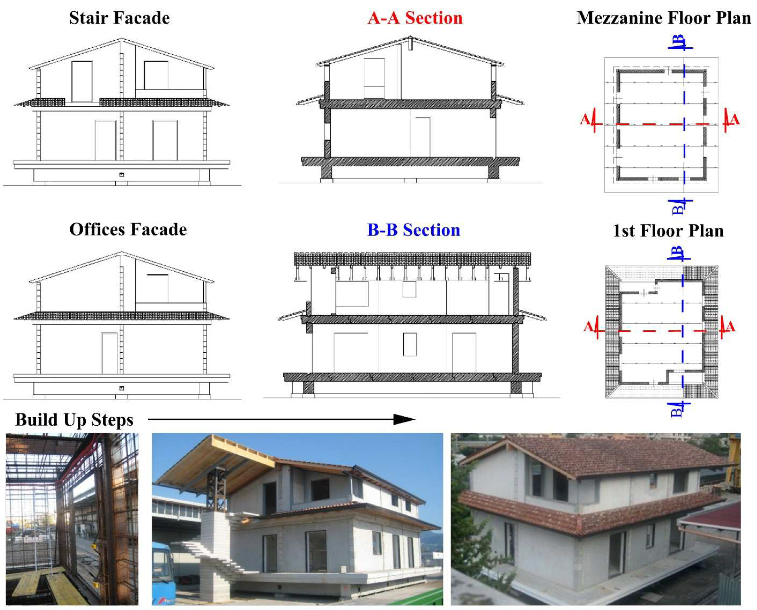
The experimental investigation focused on a full-scale two-storey building constructed using the composite panels previously analyzed. The building has a total floor area of 220 ${\mathrm{m}}^2$ and an overall height of 8.60 m, as illustrated in Figure 9. It is supported on eight individual foundations connected by four reinforced concrete foundation beams, each with a cross-section of 60 cm by 70 cm. The structural system incorporates “male-female” mechanical joints at several interfaces, including foundation-to-panel, slab-to-foundation, and panel-to-panel connections. These interlocking joints were designed to ensure rapid assembly and structural continuity. To secure the overall integrity of the system, once the second floor was positioned, post-tensioning steel cables were inserted through vertically aligned ducts in the panels. These cables were anchored at the top slab and the foundation level using specially designed through-holes, ensuring vertical precompression and enhancing global stiffness.

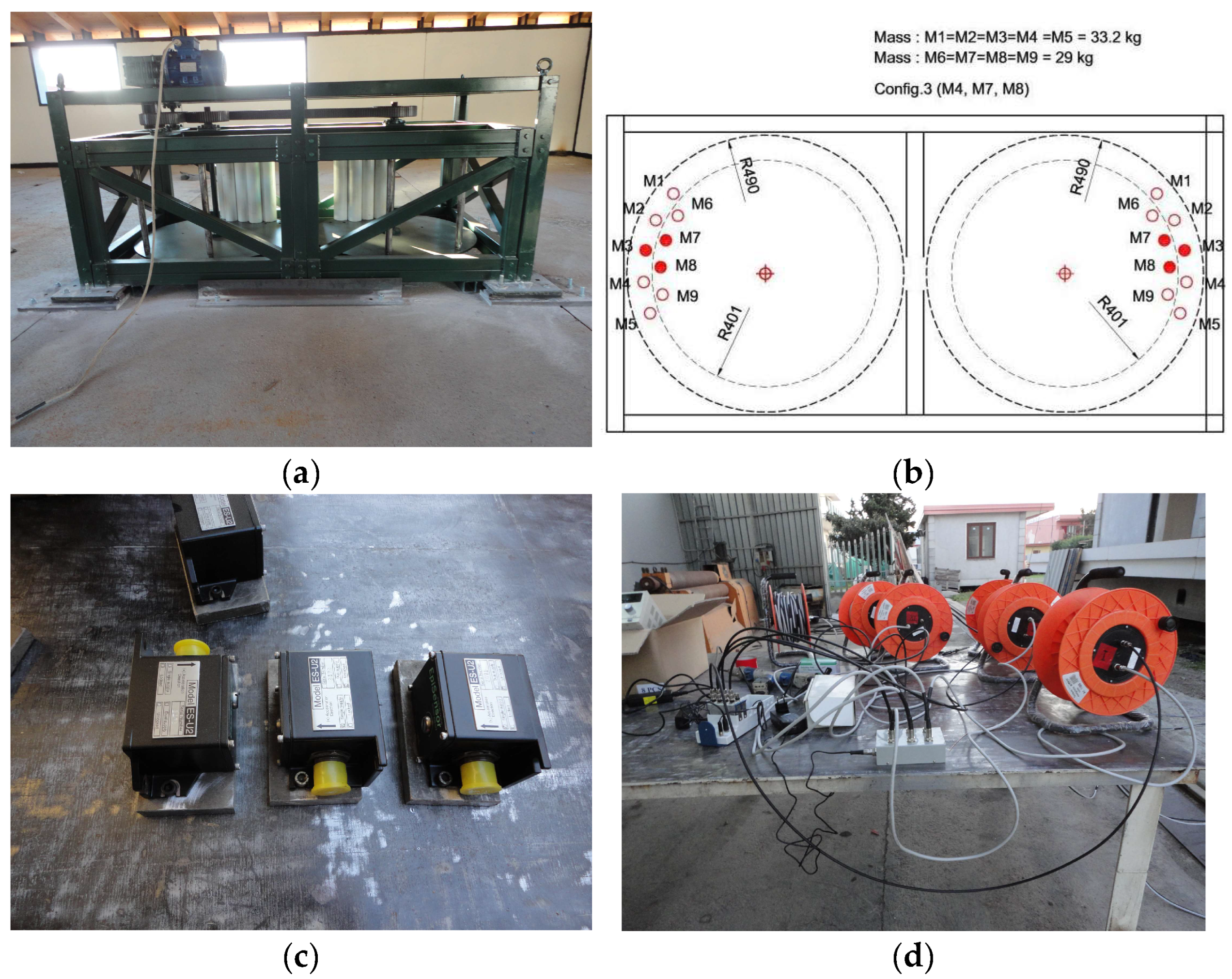
The structure was subjected to dynamic excitation along both the x and y directions. A vibrodyne system was rigidly mounted on the second floor using a configuration of steel plates and anchor bolts, as introduced above. During testing, accelerations, velocities, and displacements were recorded at various frequencies using an acquisition system that comprised five unidirectional Kinemetrics Episensor accelerometers. These sensors were strategically positioned at the four corners of the second-floor slab. Data processing focused on identifying the excitation period producing the maximum displacements in both directions. To accurately determine the building’s natural vibration frequency, the influence of the applied forcing function was removed from the measured response.

For each phase, the acceleration profiles were recorded and used to reconstruct the time history of the applied sinusoidal force and the whole experimental arrangement is illustrated in Figure 10.

4.1. Dynamic Simulation Using Equivalent Panels

To assess the predictive capacity of the equivalent homogenized panel models, a full-scale FE simulation of the two-storey structure was carried out. The simulation adopted the previously calibrated values of equivalent elastic modulus $E_{eq}$ and equivalent panel thickness ${\delta }_{eq}$, derived analytically in previous section.

In the FE model, the composite floor panels of the first and second storeys, originally 32 cm and 26 cm thick, respectively, were replaced by homogeneous layers having equivalent mechanical properties. Specifically, the panels were modeled with $\delta$_eq $=16.51 \mathrm{c}\mathrm{m}$ of thickness for the first floor, and with $\delta$_eq $=12.20 \mathrm{c}\mathrm{m}$ for the second floor. The model geometry matched the actual dimensions of the experimental building and incorporated appropriate boundary conditions and mass distributions consistent with the physical setup. Figure 11a shows the final FE model of the structure, where solid tetrahedral elements were employed for both the structural panels and the frame components.

A modal analysis was performed to extract the dynamic characteristics of the system. The first mode shape, corresponding to the dominant vibration along the x-direction, is depicted in Figure 11b, while the second significant mode in the y-direction is shown in Figure 11c. These mode shapes correspond to the expected translational behavior of the full structure under harmonic forcing applied via the Vibrodyne actuator.

To provide a clearer overview of the experimental configuration, the main dynamic test parameters are summarized in

Table 3. Main experimental parameters adopted in the dynamic characterization.

Parameter	Range/Value	Unit	Description
Period	0.28–0.32	s	Range of dominant vibration periods identified during testing
Main frequency	3.15	Hz	Fundamental excitation frequency of the vibrodyne system
Maximum acceleration	0.20	m/s2	Peak acceleration recorded during harmonic excitation
Maximum displacement	0.32	mm	Maximum measured displacement at resonance
Sampling rate	200	Hz	Data acquisition rate of the vibrodyne sensors
Instrument accuracy	±0.01	mm	Accuracy of displacement sensors (LVDTs)

. These values describe the excitation and measurement characteristics of the vibrodyne-based modal tests performed on the two-storey prototype. It is worth noting that the dynamic analysis supports the static and equivalent stiffness investigation presented in the previous sections and was mainly used for validation of the global response.

4.2. Comparison of Simulated and Experimental Response

The fidelity of the FE simulation using the equivalent panel properties was evaluated by comparing the numerically predicted dynamic response against the experimental measurements obtained from the Vibrodyne-based modal tests. The comparison focused on both the vibration periods and the amplitude of structural displacements under harmonic excitation.

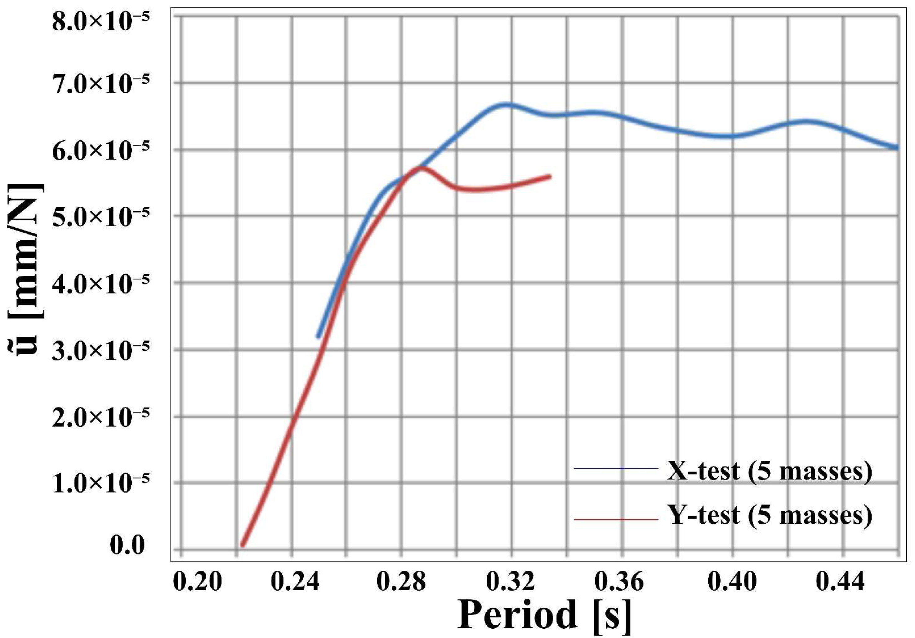
As previously discussed, the dynamic testing of the full-scale structure revealed that the maximum average displacements occurred at a forcing period of T = 0.286 s, corresponding to a dominant frequency of excitation. At this period, the recorded peak displacements were 3.45 mm in the x-direction and 3.37 mm in the y-direction, as illustrated in Figure 12, which reports the normalized displacement ($\tilde{u}=u/F$) with respect to the excitation period (T). The dynamic tests were performed using the Vibrodyne loaded with five masses per rotating disk in both X and Y directions.

The FE simulation yielded remarkably consistent results. The first mode of vibration, oriented in the x-direction, had a period of T₁ = 0.321 s, while the third mode, governing the y-direction response, showed a period of T₃ = 0.286 s. These values closely match the experimentally observed dynamic characteristics, particularly in the y-direction where the agreement is exact. The slight overestimation in the x-direction mode period (approximately 11%) may be attributed to simplifications in modeling non-structural mass distributions and connection stiffness.

Overall, the comparison confirms that the use of homogenized panels with equivalent elastic properties provides a valid and computationally efficient strategy for replicating the global dynamic behavior of complex modular systems. The simulation accurately reproduces both the natural frequencies and the displacement amplitudes observed in the full-scale experimental setup, thereby validating the analytical formulation developed in a previous section and supporting its use in future structural analysis of similar composite buildings.

5. Parametric Dataset Generation

To support surrogate modeling of composite panel behavior, a structured dataset was generated through a systematic analytical formulation, as defined in the framework of Section 3.3. Specifically, Equations. In this regard, Equations (4) and (5) were used to extract the equivalent elastic modulus $E_{eq}$ and equivalent thickness ${\mathsf{\delta }}_{eq}$ from bending and shear displacements computed through FE simulations. The dataset serves as the foundation for training ML models capable of predicting equivalent structural properties from arbitrary panel configurations.

A total of 218 unique parametric cases were developed to cover a broad range of geometrical, material, and reinforcement conditions. Each configuration was modeled using a full 3D FE mesh based on the assumptions and modeling approach detailed in Section 3. The models were implemented in the Ansys Multiphysics environment using the APDL scripting language, which enabled automated geometry construction, meshing, material assignment, boundary condition setup, and load application for each variant.

All configurations were subjected to a consistent load of 490.5 kN applied in accordance with the same boundary and loading conditions used in the experimental calibration phase. Following each simulation, the resulting displacements under both bending ($u_b$) and shear ($u_s$) loads were extracted at the panel centroid. These displacements were then used as inputs to a custom Python routine implementing the analytical homogenization equations. The script automatically calculated the corresponding equivalent elastic modulus and thickness for each case, ensuring uniform and repeatable data processing across the dataset.

The parametric ranges were selected to reflect practical design limits of prefabricated modular panels, ensuring that the surrogate model learns realistic stiffness–geometry interactions. The variables were grouped into geometric, material, and reinforcement categories, as summarized in

Table 4. Summarizes the main parameters included in the dataset.

Category	Parameter (Symbol)	Unit	Range/Levels	Physical Role
Geometry	Panel height (H), length (L), core thickness (tm), face thickness (tt = tb)	mm	H: 1500–2800; L: 2000–2800; tm: 60–100; tt: 100–160	Define global slenderness and bending–shear contribution
Material	Core modulus (Em), face modulus (Et = Eb)	MPa	Em: 30,000–36,000; Et: 13,000–21,000	Control stiffness contrast and flexural rigidity
Reinforcement	Bar diameter (Φ), vertical spacing (iL), horizontal spacing (iH)	mm	Φ: 12–20; iL: 200–400; iH: 300–400	Influence stiffness, ductility, and crack control
Outputs	Bending and shear displacements (ub, us) → Equivalent properties (Eeq, δeq)	–	Extracted from FE response	Serve as target quantities for surrogate training

.

For the 218 complete panel models the reinforcement layout was modified by adjusting the number of vertical and horizontal bars, their spacing, and the bar diameter, within realistic structural constraints. Although no failed simulations were observed, internal consistency checks were performed to ensure that each resulting $E_{eq}$ and ${\mathsf{\delta }}_{eq}$ value corresponded to physically admissible displacement magnitudes.

Statistical characterization of the dataset confirmed broad yet balanced variability. The geometric parameters showed coefficients of variation of 0.22–0.27, while E_m and E_t exhibited moderate dispersion (COV ≈ 0.15), ensuring sufficient contrast for training without biasing the model toward extreme stiffness cases.

This dataset captures the essential coupling between geometry, material stiffness, and internal reinforcement in determining the equivalent behavior of composite panels. It provides the basis for the supervised ML strategies described in Section 6 and supports the development of predictive tools for early-stage panel design and optimization. An overview of the proposed methodology is provided in Figure 13.

6. Machine Learning Surrogate Modeling

To complement the analytical approach and further generalize the mechanical behaviour of composite panels, we integrate ML as a surrogate modeling tool [33]. The inverse equations yield equivalent parameters for a finite set of panel configurations; however, practical engineering applications often demand fast predictions across a broader design space with varying geometry, reinforcement, and material properties. This integration of physics-based inversion and machine learning represents a distinctive contribution, enabling real-time estimation of equivalent parameters directly from input configurations. ML offers a data-driven strategy to interpolate and extrapolate mechanical responses from these engineered features without rerunning analytical or experimental procedures. Against this backdrop, this section details the development, training, and evaluation of supervised ML models used to predict the equivalent elastic modulus ($E_{eq}$) and equivalent thickness (${\mathsf{\delta }}_{eq}$). We chose four ML algorithms that provide a good balance between accuracy, speed, and resilience. The selected models include Artificial Neural Networks (ANN), which are well-suited for capturing high non-linear patterns; Random Forest (RF), known for its stability and resistance to overfitting in small-to-medium datasets; Extreme Gradient Boosting (XGBoost), which offers high predictive power through sequential learning and regularization; and Extra Trees Regressor (ETR), which enhances variance reduction by introducing additional randomization in the tree-building process. Each algorithm was tuned using a hyperparameter optimization procedure. Performance was evaluated under five-fold cross-validation to ensure generalizability. The complete workflow was implemented in Python using the Scikit-learn [34] and XGBoost [35] libraries, enabling reproducible and scalable model development.

6.1. Data Preparation, Scaling, and Machine Learning Algorithms

The training dataset was generated from the parametric numerical study of Section 4. It includes 15 input features including core thickness, lightweight concrete thickness, Young’s modulus of the core, Young’s modulus of the lightweight layer, panel height, panel length, reinforcement bar diameter, internal longitudinal spacing, side spacing, transverse spacing, number of longitudinal bars, number of transverse bars, applied load, bending displacement, and shear displacement. All geometric quantities are expressed in millimeters (mm), material stiffness values in megapascals (MPa), and load in Newtons (N). The two target outputs, ${\delta }_{eq}$ and $E_{eq}$, were computed for each sample using the analytical inverse formulae derived in Section 5. Prior to training, all input features were scaled using a StandardScaler [35] to improve model convergence and avoid feature dominance. Since the parametric dataset was numerically generated under predefined physical limits, no outliers were present. Feature standardization was performed using the StandardScaler to remove the mean and scale to unit variance. This method was preferred over Min–Max normalization as it preserves the relative feature variance and enhances convergence for algorithms such as ANN and XGBoost. Two separate scalers were applied to the target variables to account for differences in numerical range and variance.

Four supervised machine-learning algorithms were implemented and compared. A feedforward Artificial Neural Network (ANN) [36] was trained using the MLPRegressor class [34], with architecture and learning parameters optimized through grid search and early stopping [37,38] to prevent overfitting. The Random Forest (RF) [39,40] model, based on ensembles of decision trees trained on bootstrapped subsets, was tuned by cross-validation to balance bias and variance. The Extreme Gradient Boosting (XGBoost) algorithm [35,41] was used as an enhanced gradient-boosted ensemble with regularized loss minimization, where learning rate, tree depth, and regularization coefficients were optimized to achieve stable generalization. Finally, the Extra Trees Regressor (ETR) [42] was trained as a randomized ensemble using the entire dataset without bootstrapping, introducing random split thresholds to reduce variance and improve predictive robustness.

6.2. Model Training and Evaluation Strategy

To ensure that all algorithms were compared fairly and consistently, all models were trained on the same dataset using the same preprocessing, cross-validation, and evaluation methods. We first split the whole dataset into two groups: one for training and one for testing. A stratified 70/30 split was used. This distribution ensured there was enough variety for training while keeping a separate group for the final generalization evaluation. We set up a separate grid of hyperparameters for each ML model: ANN, Random Forest, XGBoost, and Extra Trees (see

Table 5. Hyperparameter Tuning—Search Ranges and Final Selected Values.

Model	Hyperparameter	Search Space	Final Selected Value
ANN	Hidden Layers	(64, 32), (128, 64, 32), (256, 128, 64)	(256, 128, 64)
	Learning Rate Init	0.001, 0.01, 0.1	0.001
	Alpha (L2 penalty)	0.0001, 0.001, 0.01	0.0001
RF	n-estimators	100, 200, 300	100
	max-depth	None, 5, 10, 20	10
	min-samples-split	2, 10, 20	10
	min-samples-leaf	1, 5, 10	1
	Bootstrap	True, False	True
XGBoost	colsample-bytree	0.8, 1.0, 1.2	0.8
	Gamma	0, 0.01, 0.1	0
	learning-rate	0.01, 0.1, 0.2, 0.3	0.2
	max-depth	2, 4, 6	2
	min-child-weight	1, 4, 7	4
	n-estimators	50, 100, 200	200
	reg-alpha	0.01, 0.1, 1.0	0.01
	reg-lambda	0, 0.001, 0.01, 0.1	0.001
	Subsample	0.8, 1.0, 1.2	0.8
ExtraTrees	n-estimators	100, 200, 300	200
	max-depth	None, 10, 20, 30	None
	min-samples-split	2, 10, 20	2
	min-samples-leaf	1, 4, 10	1
	Bootstrap	False, True	True

for more information). A Grid Search CV method was used to search the whole parameter space, utilizing five-fold cross-validation and the $R^2$ score as the optimization metric. This approach was repeated separately for each of the two target variables.

After finding the best hyperparameter settings for each model, the corresponding estimator was retrained on the entire training set and saved as a .joblib file. In addition to tracking the best score, fold-wise predictions were generated and exported for detailed error analysis. Specifically, for each of the five folds, the trained model predicted outcomes on the validation subset, and the resulting predictions were saved alongside the true values to Excel files for further interpretation. Performance metrics including $R^2$, Mean Absolute Error (MAE), and Root Mean Square Error (RMSE) (

Table 6. Formulas and descriptions of the evaluation metrics used to assess model performance: Coefficient of Determination (${\mathrm{R}}^2$) (Values closer to 1 indicate better predictive performance), Mean Absolute Error (MAE) (Unlike RMSE, it gives equal weight to all errors and is less affected by outliers), and Root Mean Square Error (RMSE) (penalizing large errors more than MAE).

Metric	Formula	Description
${\mathrm{R}}^2$	$R^2=1-{\displaystyle \frac{{\sum }_{i=1}^n{\left(y_i-\widehat{y_i}\right)}^2}{{\sum }_{i=1}^n{\left(y_i-\overline{y_i}\right)}^2}}$	Proportion of variance in the observed data explained by the model.
MAE	$MAE={\displaystyle \frac{1}{n}}{\displaystyle \sum _{i=1}^n}|y_i-\widehat{y_i}|$	MAE quantifies the average absolute difference between predicted and actual values.
RMSE	$RMSE=\sqrt{{\displaystyle \frac{1}{n}}{\displaystyle \sum _{i=1}^n}{\left\{y_i-\widehat{y_i}\right)}^2}$	Reflects the square root of the average squared differences.

) were calculated for each fold and aggregated to report mean performance for each model. This unified training pipeline was implemented in Python using Scikit-learn for preprocessing, model evaluation, and pipeline management, and XGBoost was used for gradient boosting implementations. The complete pipeline ensures transparency, comparability, and full reproducibility from preprocessing to model deployment.

This modeling framework provides a complete surrogate prediction system for estimating mechanical response in composite panel systems by combining several algorithmic approaches and carefully optimizing hyperparameters. The final models are also integrated into a practical GUI tool described in the last section.

6.3. Machine Learning Analysis Results

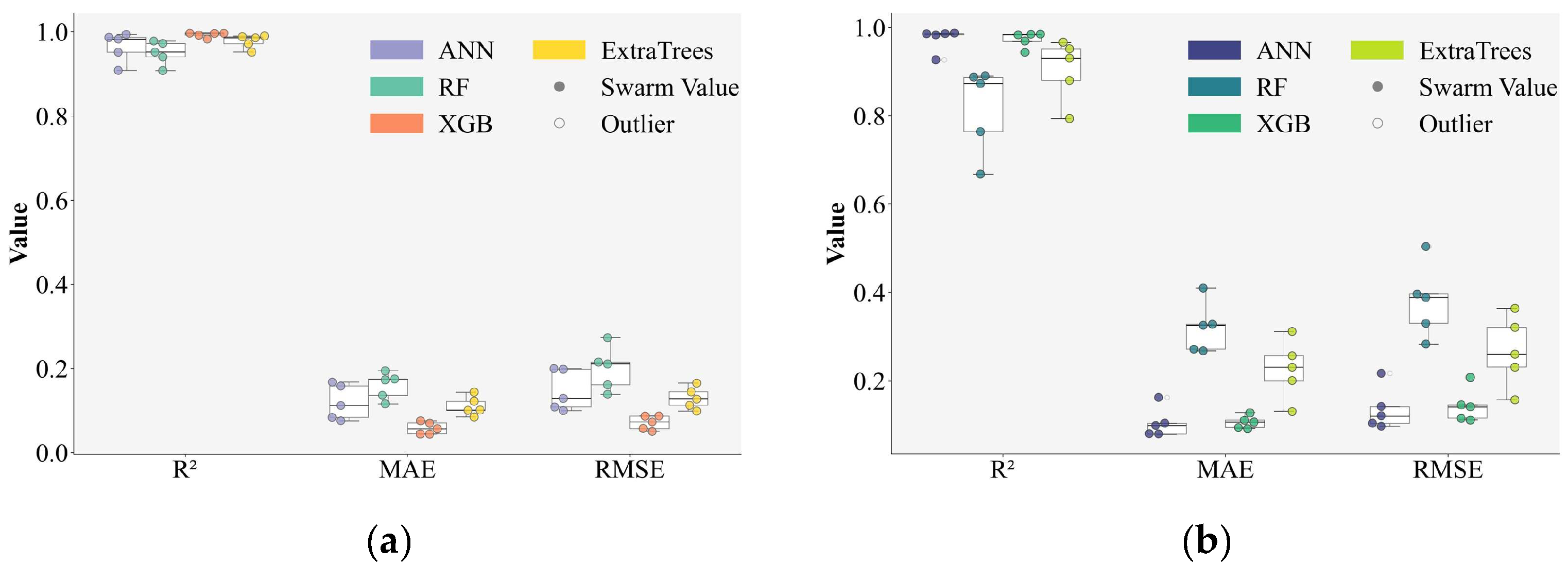
The comparative analysis of fold-wise performance across both target properties including equivalent thickness (${\delta }_{eq}$) and equivalent Young’s modulus ($E_{eq}$) shows that XGBoost and ANN consistently surpassed RF and ExtraTrees in terms of accuracy and stability.

For equivalent thickness (Figure 14a), XGBoost showed better performance, achieving near-perfect R² scores across all folds with minimal MAE and RMSE dispersion. This indicates its high precision in capturing the structured nonlinearity of the analytical surface. ANN also performed well, particularly in folds with regular feature distributions, though slight fold-to-fold sensitivity suggests a higher dependency on initialization and optimization dynamics. ExtraTrees showed competitive ${\mathrm{R}}^2$ values but with more dispersed errors, likely due to its fully randomized split strategy. RF consistently trailed behind, even if it was reliable, which showed limitations in modeling sharp transitions in the input–output relationship.

For equivalent Young’s modulus (Figure 14b), ANN was the best model, with high ${\mathrm{R}}^2$ and low error metrics across most folds, except for one moderate outlier. Its ability to approximate smooth, stiffness-driven mappings appears well-suited to this prediction task. XGBoost came in second, with high consistency but slightly greater bias in some folds. ExtraTrees and RF, on the other hand, showed larger variability and higher error ranges, which means a less stable generalization capacity for stiffness estimation.

Figure 15 shows how well all of the models predicted the two mechanical targets, ${\mathsf{\delta }}_{eq}$ and $E_{eq}$. Based on Figure 15a, XGBoost regularly achieved ${\mathrm{R}}^2$ values close to perfect $(>0.99$) on training, test, and full datasets for both targets, beating other models. ANN and ExtraTrees both did well for ${\mathsf{\delta }}_{eq}$, but RF’s test accuracy for $E_{eq}$ dropped significantly (${\mathrm{R}}^2=0.832$), which means poor generalization for stiffness prediction. According to Figure 15b, XGBoost again led with the lowest errors (0.339 mm for ${\mathsf{\delta }}_{eq}$ and 98.78 MPa for $E_{eq}$), showing its robustness. ExtraTrees and ANN performed well overall but showed signs of overfitting, especially for $E_{eq}$. For example, ExtraTrees had a low training MAE for ${\mathsf{\delta }}_{eq}$ (0.005 mm), which rose to 1.62 mm on the test set. The RMSE results from Figure 15c further confirm these trends. XGBoost maintained the lowest RMSE across both targets (0.650 mm and 179.33 MPa), followed by ANN. RF displayed the highest RMSE for $E_{eq}$, on the test set (940 MPa). Accurate prediction of ${\mathsf{\delta }}_{eq}$ and $E_{eq}$ is important for reliable modeling of composite panels. XGBoost proved the most effective, while ANN remains a strong alternative when properly tuned. RF and ExtraTrees were less effective in capturing coupled geometrical–mechanical relationships in this context.

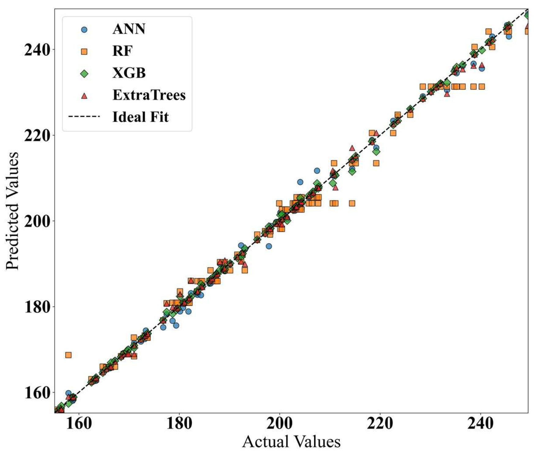
Figure 16 shows the predicted values of ${\mathsf{\delta }}_{eq}$ compared to the actual values across all instances, showing how well the model matches the ideal 1:1 line. All four models were quite good at predicting, but XGBoost was the best across the board, showing that it had minimal bias and was able to generalize well. ANN and ExtraTrees likewise stayed close to the diagonal, while RF was more spread out, especially at lower ${\mathsf{\delta }}_{eq}$ values (less than 200 mm), which shows that it doesn’t generalize as well.

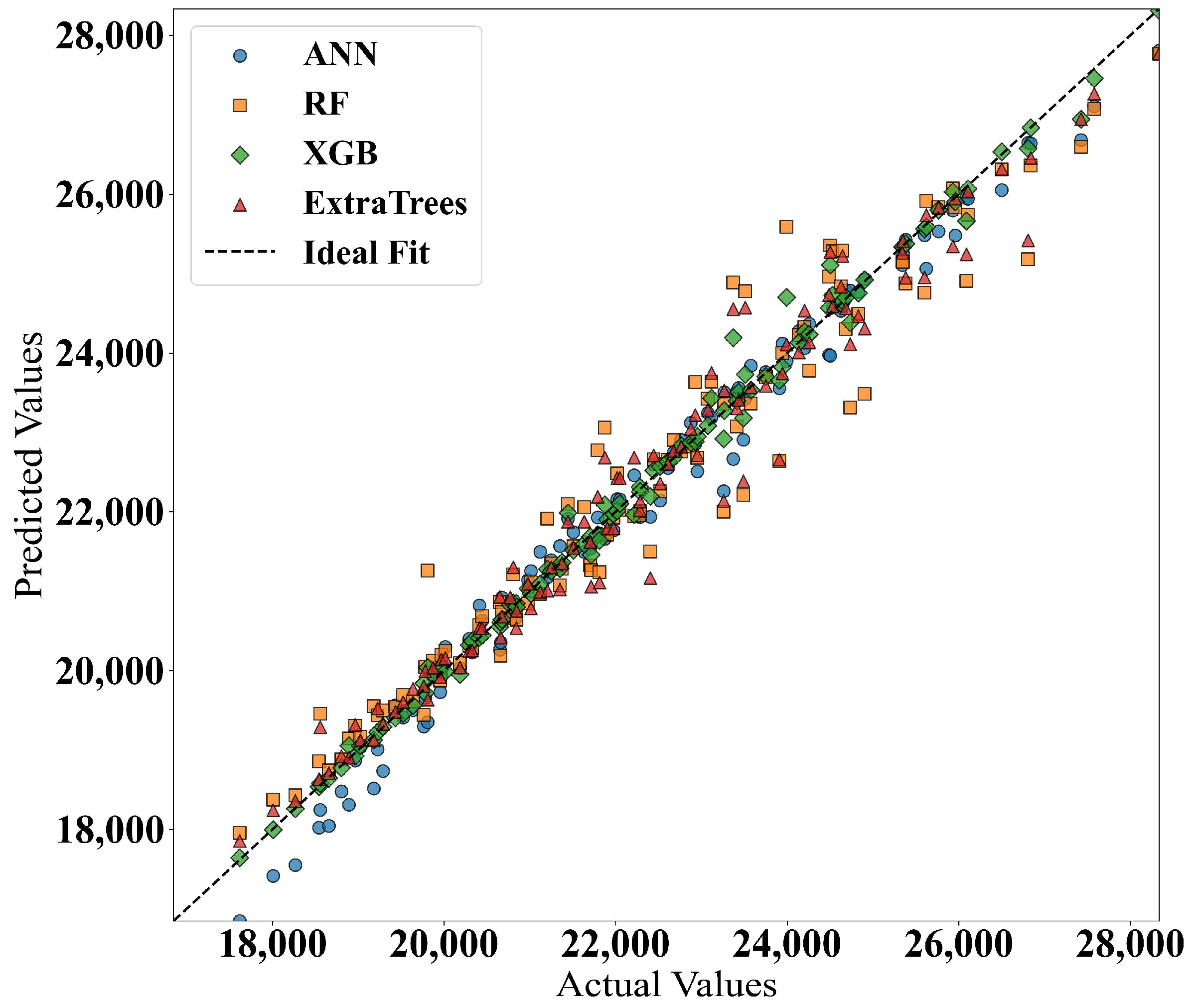
Figure 17 shows the predicted versus actual values of $E_{eq}$, which shows important differences in model behaviour. XGBoost and ExtraTrees consistently followed the ideal 1:1 line closely across the whole modulus range (17,500–28,000 MPa). This shows that they learned stiffness trends well by managing feature interactions. ANN also performed well but slightly underestimated lower modulus values, possibly due to local data sparsity or activation saturation effects. On the other hand, RF showed noticeable spread in the upper range, confirming its reduced capacity to generalize non-linear stiffness patterns.

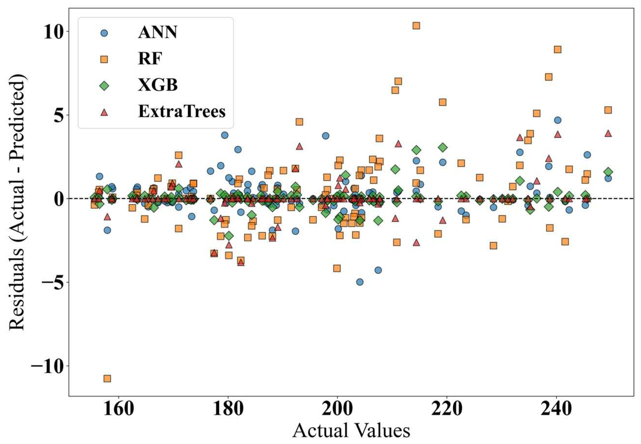
Figure 18 examines residual distributions across predicted ${\mathsf{\delta }}_{eq}$ values to give insights into local prediction fidelity. XGBoost and ExtraTrees had tight, symmetrical residuals that were centred around zero. This showed that they were good at generalizing and handling local variances. This stability is attributed to their ensemble structures, which effectively capture complex feature interactions. On the other hand, ANN showed moderate variance and isolated underestimations, likely tied to non-linear zones with sparse data. At higher ${\delta }_{eq}$ values, RF consistently under-predicted, which suggests difficulties in modelling flexible panel configurations due to limited adaptability of axis-aligned splits. Since ${\delta }_{eq}$ affects serviceability and deformation-based design, it is important to keep residual bias as low as possible. The better residual behaviour of XGBoost and ExtraTrees confirms their suitability for reliable surrogate modelling in structural applications.

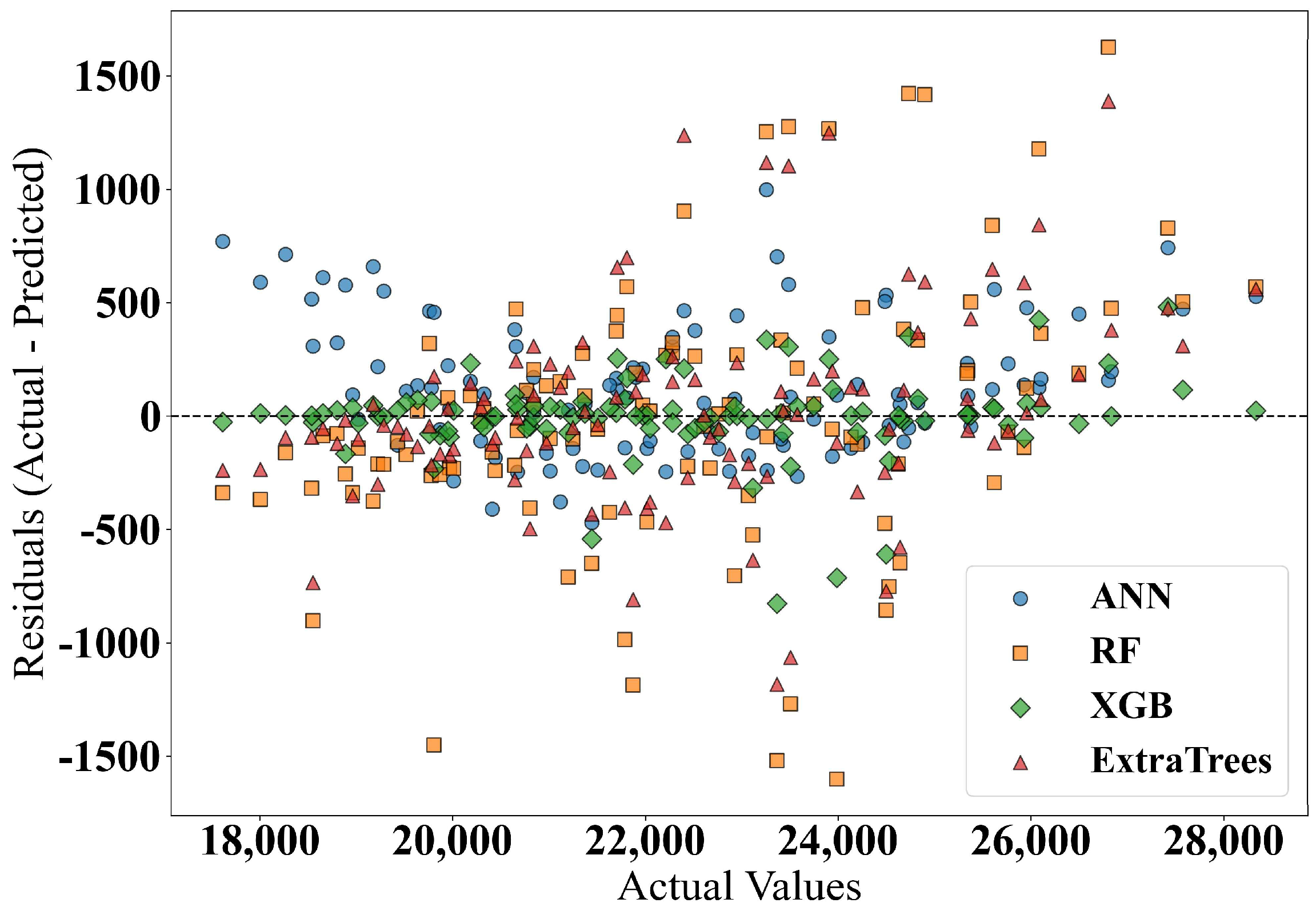
Figure 19 shows the residual distributions for anticipated equivalent stiffness ($E_{eq}$), which show key differences in how the models behaviour. XGBoost has the most consistent and symmetrical residuals, which shows that it can capture the non-linear relationships between input features. ExtraTrees and RF, on the other hand, display broader residual dispersion, especially in higher stiffness regions. This means that they are less generalizable and may overfit certain configurations. ANN performs reasonably but slightly over-predicts in stiffer assemblies. This could be because it is sensitive to early convergence or limited high-modulus training data. The results confirm that boosting-based models, especially XGBoost, are better suited for representing composite stiffness trends.

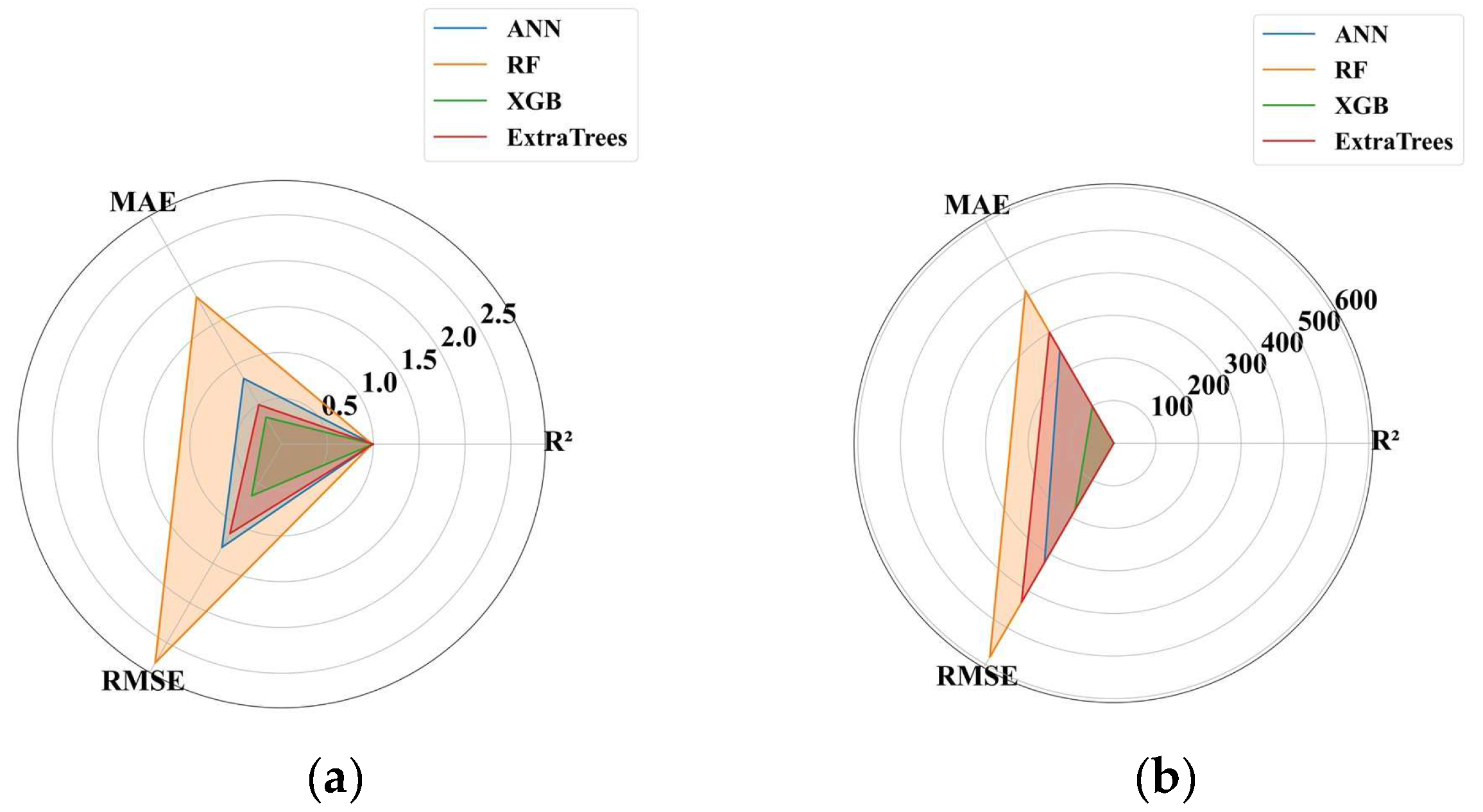
Figure 20a shows comparison of model performance for predicting ${\mathsf{\delta }}_{eq}$ across the entire dataset. The plot illustrates the balance between ${\mathrm{R}}^2$, MAE, and RMSE for each ML model. XGBoost and ExtraTrees show compact profiles, indicating low errors and high predictive power. In contrast, the RF model shows wider spread, particularly in RMSE, highlighting reduced robustness. ANN achieves competitive MAE but with larger variance, suggesting sensitivity to localized panel configurations. Figure 20b shows comparison of model performance for predicting $E_{eq}$ across the entire dataset. The XGBoost model displays the most compact and balanced radar shape, combining high accuracy (${\mathrm{R}}^2$) with low MAE and RMSE. ExtraTrees performs similarly but with slightly higher dispersion in error metrics. The ANN model shows moderate performance but with increased error spread, while RF underperforms due to its inability to generalize well under varying stiffness and reinforcement layouts. The radar profiles effectively reflect the trade-offs between prediction error and generalization capacity in modeling complex structural behaviors.

Figure 21 presents SHapley Additive exPlanations (SHAP)-based interpretability analysis. SHAP quantifies the contribution of each input feature to the model’s output by computing local, model-agnostic attributions grounded in game theory [43]. For clarity and interpretability, only the seven most influential features are shown in Figure 21 and Figure 22. For ${\mathsf{\delta }}_{eq}$ (Figure 21a), the thickness of the lightweight concrete layer emerges as the most important feature, followed by the core thickness and panel height. This shows that deformability is primarily governed by the panel’s layered geometry. Core modulus and inversion displacements contribute minimally, indicating that ${\mathsf{\delta }}_{eq}$ is more sensitive to geometrical than mechanical properties. For $E_{eq}$ (Figure 21b), core thickness and core elastic modulus are the leading predictors, aligning with their direct role in defining panel stiffness. Geometric features such as panel height and length also show moderate influence. Notably, the lightweight layer’s thickness-dominant in ${\mathsf{\delta }}_{eq}$ prediction has less impact on stiffness, emphasizing a clear separation between deformation- and stiffness-driving factors. These results reinforce the model’s ability to reflect meaningful mechanical dependencies through learned patterns.

Figure 22 summarizes the global feature importance based on SHAP values for both target outputs. For ${\mathsf{\delta }}_{eq}$, the lightweight concrete thickness emerges as the dominant contributor, accounting for 44.6% of the total importance. Combined with panel height (32.7%), these geometric features explain over 75% of the model’s predictive power, showing how important structural layout is in controlling deformability. Mechanical properties like core modulus and displacement inputs contribute marginally, indicating localized or case-specific effects. On the other hand, the feature importance for $E_{eq}$ is more evenly distributed. Panel height, core modulus, panel length, and bending displacement each contribute comparably (17–22%), showing a multi-variable dependency that captures both geometric configuration and material stiffness. Notably, the importance of lightweight concrete thickness drops to just 6.1%, which shows its minimal role in stiffness prediction. This divergence in SHAP profiles confirms that the models differentiate between geometry-driven and stiffness-driven targets, effectively learning the distinct physical mechanisms embedded in the inversion formulation.

As already noted, the experimental campaign was limited to a few full-scale specimens because of the high cost and complexity of testing. To address this, validated numerical and analytical models were employed to generate additional training data that remained consistent with the measured experimental responses. Several strategies were applied to mitigate overfitting, including five-fold cross-validation, hyperparameter regularization, and model interpretability analysis through SHAP values. The latter confirmed that the most influential features such as panel height, core modulus, and lightweight layer thickness, corresponded to physically meaningful parameters, supporting the reliability of the learning process. Although this combined approach effectively reduces overfitting risk within the defined design space, future work will focus on expanding the experimental database to further enhance the generalization capacity of the proposed surrogate models.

7. Graphical Interface for Predicting Equivalent Structural Properties

To facilitate the practical deployment of the machine learning models developed in this study, an interactive graphical user interface (GUI) was implemented using the Streamlit framework [44]. The objective of this interface is to allow structural engineers and researchers to predict the ${\mathsf{\delta }}_{eq}$ and $E_{eq}$ of composite panel configurations without requiring any programming background or ML expertise. The application bridges the gap between advanced data-driven modeling and design workflows by offering an accessible prediction tool. The GUI integrates two independently optimized models, both trained using the XGBoost algorithm and fine-tuned via GridSearchCV, for predicting the equivalent mechanical properties derived from the parametric study. The trained models were saved alongside their respective input/output scalers using the .joblib format to ensure consistent normalization and inverse transformations. At runtime, these assets are loaded dynamically and retained in memory, enabling fast, responsive inference for both single and batch predictions. The batch-mode function allows the evaluation of multiple panel configurations within seconds. All trained models are pre-loaded in memory, resulting in an average runtime of about 0.05 s per single prediction and less than 2 s for typical batches of 100 records. Before processing, the application automatically verifies the uploaded Excel file to ensure that all 15 input columns are present and correctly labeled, providing user feedback when inconsistencies are detected. The application accepts 15 input features that describe key material, geometric, and reinforcement-related parameters of the composite panel system. These include concrete layer thicknesses, respective Young’s moduli, overall panel dimensions, reinforcement arrangement details (e.g., bar diameters, spacing, and layout), and applied mechanical loading conditions. The layout is modularly structured across four expandable panels, categorizing inputs into material properties, geometry, reinforcement layout, and load–displacement characteristics. This layout improves navigability while maintaining domain-specific clarity.

Once the “Predict Outputs” button is triggered, the entered data are automatically validated, scaled, and passed through the respective ML pipelines. The final predicted values for ${\mathsf{\delta }}_{eq}$ and $E_{eq}$ are displayed in engineering units (mm and MPa), with controlled formatting to ensure numerical interpretability. Additionally, the GUI provides the option to download a complete summary of the input parameters and output predictions in Excel format, supporting traceability and facilitating engineering documentation or design iteration logging. Beyond individual predictions, the interface includes a batch mode for file-based inference. Users can upload Excel files containing multiple input records, and the app will return a full set of predictions with minimal delay. This functionality is particularly useful for performing systematic design explorations or analyzing large sets of parametric design alternatives. The front end was deliberately kept lightweight and intuitive, while preserving technical depth. Informative headers, unit-aware input fields, and consistent visual feedback help maintain scientific accuracy without overwhelming the user. Overall, this GUI translates the model’s analytical capabilities into a deployable tool that is both accessible and technically rigorous. Figure 23 illustrates the deployed Streamlit-based GUI, showing three main sections: the input interface where users define material properties and geometric characteristics of the panel, the reinforcement layout and loading/displacement section used to complete the feature configuration, and the output and export area, including real-time predictions of ${\delta }_{eq}$ and $E_{eq}$ along with batch processing functionality. The application is available at [45].

In addition to flexibility, the main advantage of using machine learning in this framework lies in its computational efficiency. Once trained, the models can predict equivalent panel properties within milliseconds, avoiding the need for repeated FE analyses or iterative calibration. This approach significantly reduces the numerical cost while maintaining physical consistency, as also observed in surrogate-assisted studies for composite materials [46].

8. Conclusions

This study developed and validated a comprehensive hybrid framework for the mechanical characterization and surrogate modeling of composite structural panels. The originality of this study lies in establishing a unified and validated framework that merges experimental, analytical, and data-driven modeling into a single consistent methodology. The composite panels were first characterized through controlled bending and shear experiments, enabling the quantification of their mechanical behavior. An analytical homogenization procedure was then applied to calculate equivalent elastic modulus and thickness from displacement data, accounting for both bending and shear contributions. These equivalent parameters were validated through calibrated FE simulations and integrated into a two-storey structural model. Dynamic testing of the assembled building under harmonic excitation applied via a vibrodyne demonstrated strong agreement between measured and simulated responses. Modal periods in both directions matched within 10%, confirming the reliability of the homogenized panel formulation.

The mechanical interpretation of these results indicates that the layered concrete configuration, together with the steel frame and internal rebars, effectively transfers both flexural and shear stresses across the interfaces, behaving as a continuous composite system. The derived equivalent stiffness reflects the combined role of the lightweight layers in limiting deformation and the high-strength core in sustaining the main load.

To generalize the approach, a parametric dataset was generated by varying material and geometric parameters across 218 representative panel configurations. Each configuration was processed through the analytical equations to derive equivalent properties. These served as the training targets for multiple machine learning models. A graphical user interface was developed to let instant prediction and design assistance.

In summary, this work delivers a validated and extensible methodology for modelling, predicting, and deploying composite panel systems. Mechanically, the results show that the bending stiffness is primarily governed by the concrete core thickness and its modulus, while the shear flexibility depends more on the outer lightweight layers and their interaction with the steel frame. The equivalent panel model thus captures the true stiffness hierarchy among materials and provides realistic global behavior under dynamic loads. The homogenized panel model accurately replicated the dynamic response of the actual building, including mode shapes, modal periods, and displacement magnitudes under harmonic forcing, allowing for full-scale validation. This confirms that the proposed homogenization is not merely numerical fitting but a physically meaningful representation of stress transfer and deformation mechanisms within the composite system.

The composite panels can be modelled as equivalent slab–plate elements, with equivalent thicknesses between 12.20 cm and 16.51 cm (first floor) and between 26 cm and 32 cm (second floor), enabling fast and accurate simulations. Moreover, experimental results confirmed that mounting tolerances in panel joints enhanced energy dissipation, mimicking monolithic behaviour and improving seismic performance. Finally, an efficient surrogate modelling, trained on the parametric dataset can rapidly predict equivalent modulus and thickness with high accuracy, without the need for repeated simulations or experiments. The surrogate’s success is mainly attributed to its ability to preserve the physical consistency of the analytical model while providing near-instant numerical predictions. This integration bridges the gap between detailed mechanics and practical design use. Furthermore, combining analytical formulation with data-driven methodologies, an engineering-ready and user-friendly graphical unit interface (GUI) was built to support direct input of panel properties and instant prediction of equivalent parameters, integrating structural mechanics and Machine Learning to offer interpretable, efficient, and reliable tools for modern structural engineering.

Overall, the proposed approach demonstrates that data-driven homogenization can capture the essential mechanics of layered concrete–steel systems while reducing the computational burden of traditional FE calibration. The observed stiffness distribution and damping behaviour provide clear cause–effect insights into how layer configuration and reinforcement influence global response. Future research may expand this framework to account for non-linear, seismic, or thermal behaviour.

References

1. De Silva, C.W. Vibration Monitoring, Testing, and Instrumentation; CRC Press: Boca Raton, FL, USA, 2007. [Google Scholar] [CrossRef]
2. Ewins, D.J. Modal Testing: Theory, Practice and Application; John Wiley & Sons: Hoboken, NJ, USA, 2009. [Google Scholar]
3. Cennamo, C.; Gesualdo, A.; Monaco, M. Shear plastic constitutive behavior for near-fault ground motion. J. Eng. Mech. 2017, 143, 04017086. [Google Scholar] [CrossRef]
4. Palladino, S.; Esposito, L.; Ferla, P.; Totaro, E.; Zona, R.; Minutolo, V. Experimental and numerical evaluation of residual displacement and ductility in ratcheting and shakedown of an aluminum beam. Appl. Sci. 2020, 10, 3610. [Google Scholar] [CrossRef]
5. Zona, R.; Esposito, L.; Ferla, P.; Palladino, S.; Totaro, E.; Minutolo, V. Lower bound limit analysis of parabolic domes based on spherical analytical solution. Int. J. Adv. Res. Eng. Technol. 2020, 11, 59–79. [Google Scholar]
6. Lalanne, C. Sinusoidal Vibration; CRC Press: Boca Raton, FL, USA, 2002. [Google Scholar] [CrossRef]
7. Li, Z.; Zhang, S.; Zhou, Y.; Wu, W.; Tu, L.; Liu, J. Calibrating nonlinearity coefficients of a nano-g accelerometer by dual-frequency excitation on a shaker. Measurement 2024, 225, 114016. [Google Scholar] [CrossRef]
8. Yang, M.; Phung, B.T. Motor winding insulation degradation under repetitive voltage pulses. IEEE Access 2024, 12, 77658–77674. [Google Scholar] [CrossRef]
9. Dash, B.; Mahapatra, T.R.; Mishra, P.; Mishra, D.; Mahmoud, S.R. A Review of Computational Methods for Vibroacoustic Analysis of Advanced Material Structures. Arch. Comput. Methods Eng. 2025, 32, 2187–2211. [Google Scholar] [CrossRef]
10. Jefferson, A.; Sain, M.; Ramakrishna, S.; Jawaid, M.; Dhakal, H.N. Environmentally friendly fire retardant natural fibre composites: A review. Int. Mater. Rev. 2024, 69, 267–308. [Google Scholar] [CrossRef]
11. Bocheński, M.; Gawryluk, J.; Kłoda, L. Experimental modal analysis of an active thin-walled composite structure. Model. Meas. Control B 2019, 88, 154–159. [Google Scholar] [CrossRef]
12. Pourkamali-Anaraki, F.; Husseini, J.F.; Pineda, E.J.; Bednarcyk, B.A.; Stapleton, S.E. Two-stage surrogate modeling for data-driven design optimization with application to composite microstructure generation. Eng. Appl. Artif. Intell. 2024, 138, 109436. [Google Scholar] [CrossRef]
13. Husseini, J.; Stapleton, S.; Carey, E.; Pineda, E.J. Microscale Constitutive Model Sensitivity on Multiscale Modeling of Fiber Reinforced Composites. In Proceedings of the AIAA SCITECH 2025 Forum, Orlando, FL, USA, 6–10 January 2025; p. 1155. [Google Scholar] [CrossRef]
14. Rainieri, C.; Fabbrocino, G.; Cosenza, E. Automated Operational Modal Analysis as structural health monitoring tool: Theoretical and applicative aspects. Key Eng. Mater. 2007, 347, 479–484. [Google Scholar] [CrossRef]
15. Rainieri, C.; Fabbrocino, G.; Cosenza, E.; Manfredi, G. Implementation of OMA procedures using LabVIEW: Theory and application. In Proceedings of the 2nd International Operational Modal Analysis Conference, Copenhagen, Denmark, 30 April–2 May 2007; Volume 30, pp. 1–13. [Google Scholar]
16. Esposito, L.; Palladino, S.; Minutolo, V. An effective free-meshing and linear Step-Wise procedure to predict crack initiation and propagation. Theor. Appl. Fract. Mech. 2024, 130, 104240. [Google Scholar] [CrossRef]
17. Arndt, C.; Crusenberry, C.; Heng, B.; Butler, R.; TerMaath, S. Reduced-dimension surrogate modeling to characterize the damage tolerance of composite/metal structures. Modelling 2023, 4, 485–514. [Google Scholar] [CrossRef]
18. Dashtgoli, D.S.; Taghizadeh, S.; Macconi, L.; Concli, F. Comparative analysis of machine learning models for predicting the mechanical behavior of bio-based cellular composite sandwich structures. Materials 2024, 17, 3493. [Google Scholar] [CrossRef] [PubMed]
19. Viotti, I.D.; Gomes, G.F. Delamination identification in sandwich composite structures using machine learning techniques. Comput. Struct. 2023, 280, 106990. [Google Scholar] [CrossRef]
20. Kamarian, S.; Teimouri, A.; Alinia, M.; Saber-Samandari, S.; Song, J.I. Machine learning for bending behavior of sandwich beams with 3D-printed core and natural fiber-reinforced composite face sheets. Polym. Compos. 2024, 45, 3043–3054. [Google Scholar] [CrossRef]
21. Mottaghian, F.; Taheri, F. Machine learning/finite element analysis—A collaborative approach for predicting the axial impact response of adhesively bonded joints with unique sandwich composite adherends. Compos. Sci. Technol. 2023, 242, 110162. [Google Scholar] [CrossRef]
22. Vaishali; Mukhopadhyay, T.; Naskar, S.; Dey, S. On machine learning assisted data-driven bridging of FSDT and HOZT for high-fidelity uncertainty quantification of laminated composite and sandwich plates. Compos. Struct. 2023, 304, 116276. [Google Scholar] [CrossRef]
23. Khan, A.; Kim, N.; Shin, J.K.; Kim, H.S.; Youn, B.D. Damage assessment of smart composite structures via machine learning: A review. JMST Adv. 2019, 1, 107–124. [Google Scholar] [CrossRef]
24. Ribeiro, R.F., Jr.; Gomes, G.F. On the use of machine learning for damage assessment in composite structures: A review. Appl. Compos. Mater. 2024, 31, 1–37. [Google Scholar] [CrossRef]
25. Modano, M.; Albo, N.; Fulgione, M.; Spizzuoco, M. Dynamical Characterization of an Innovative Building System. In Proceedings of the GIMC-SIMAI Workshop for Young Scientists, Naples, Italy, 10–12 July 2024; Springer: Cham, Switzerland, 2024; pp. 113–122. [Google Scholar]
26. Modano, M.; Fabbrocino, F.; Gesualdo, A.; Matrone, G.; Farina, I.; Fraternali, F. On the forced vibration test by vibrodyne. In Proceedings of the COMPDYN 2015—5th ECCOMAS Thematic Conference on Computational Methods in Structural Dynamics and Earthquake Engineering, Crete Island, Greece, 25–27 May 2015; pp. 209–217. [Google Scholar]
27. Modano, M.; Gesualdo, A.; Mascolo, I.; Farina, I. Dynamic testing and structural identification of innovative network structures. In Proceedings of the Atti del XXIII Convegno AIMETA, Salerno, Italy, 4–7 September 2017; Volume 3, pp. 1205–1213. [Google Scholar]
28. Palladino, S.; Fraldi, M.; Minutolo, V.; Esposito, L. Steering Cracks Via Auxetic Zebra-Composites. SSRN 2025. [Google Scholar] [CrossRef]
29. Sarfarazi, S.; Fakhraddini, A.; Modaresahmadi, K. Evaluation of panel zone shear strength in cruciform columns, box-columns and double web-columns. Int. J. Struct. Civ. Eng. Res. 2016, 5, 52–56. [Google Scholar] [CrossRef]
30. Sarfarazi, S.; Saffari, H.; Fakhraddini, A. Shear Behavior of Panel Zone Considering Axial Force for Flanged Cruciform Columns. Civ. Eng. Infrastruct. J. 2020, 53, 359–377. [Google Scholar]
31. Hu, X.; Yu, S.; Li, Y.; Liu, R.; Yu, J. Research on the influencing mechanisms of ice-filled fissures on the failure processes of tunnel specimens. Theor. Appl. Fract. Mech. 2025, 139, 105141. [Google Scholar] [CrossRef]
32. Zhang, Q.; Yu, S.; Yu, J.; Li, Y.; Xu, H.; Huang, Q. Investigating the interaction mechanisms between fissures and layers of SCB specimens using a novel layer 3D printing technology and DEM. Theor. Appl. Fract. Mech. 2025, 139, 105044. [Google Scholar] [CrossRef]
33. Mascolo, I.; Sarfarazi, S.; Modano, M. Feasible and robust optimisation of cable forces in suspended bridges: A two-stage metaheuristic approach. Mech. Res. Commun. 2025, 104, 104554. [Google Scholar] [CrossRef]
34. Pedregosa, F.; Varoquaux, G.; Gramfort, A.; Michel, V.; Thirion, B.; Grisel, O.; Blondel, M.; Prettenhofer, P.; Weiss, R.; Dubourg, V.; et al. Scikit-learn: Machine learning in Python. J. Mach. Learn. Res. 2011, 12, 2825–2830. [Google Scholar]
35. Chen, T.; Guestrin, C. XGBoost: A scalable tree boosting system. In Proceedings of the 22nd ACM SIGKDD International Conference on Knowledge Discovery and Data Mining, San Francisco, CA, USA, 13–17August 2016; pp. 785–794. [Google Scholar] [CrossRef]
36. Abdel-aziem, A.H.; Soliman, T.H.M. A multi-layer perceptron (MLP) neural networks for stellar classification: A review of methods and results. Int. J. Adv. Appl. Comput. Intell. 2023, 3, 29–37. [Google Scholar] [CrossRef]
37. Sarfarazi, S.; Mascolo, I.; Modano, M.; Guarracino, F. Application of Artificial Intelligence to Support Design and Analysis of Steel Structures. Metals 2025, 15, 408. [Google Scholar] [CrossRef]
38. Sazlı, M.H. A brief review of feed-forward neural networks. Commun. Fac. Sci. Univ. Ank. Ser. A2–A3 Phys. Sci. Eng. 2006, 50. [Google Scholar] [CrossRef]
39. Rabi, M.; Abarkan, I.; Sarfarazi, S.; Ferreira, F.V.; Alkherret, A.J. Automated design and optimization of concrete beams reinforced with stainless steel. Struct. Concr. 2025; early view. [Google Scholar] [CrossRef]
40. Sarfarazi, S.; Shamass, R.; Guarracino, F.; Mascolo, I.; Modano, M. Exploring the stainless-steel beam-to-column connections response: A hybrid explainable machine learning framework for characterization. Front. Struct. Civ. Eng. 2025, 19, 34–59. [Google Scholar] [CrossRef]
41. Sarfarazi, S.; Shamass, R.; Guarracino, F.; Mascolo, I.; Modano, M. Advanced predictive modeling of shear strength in stainless-steel column web panels using explainable AI insights. Results Eng. 2024, 24, 103454. [Google Scholar] [CrossRef]
42. Geurts, P.; Ernst, D.; Wehenkel, L. Extremely randomized trees. Mach. Learn. 2006, 63, 3–42. [Google Scholar] [CrossRef]
43. Lundberg, S.M.; Lee, S.-I. A unified approach to interpreting model predictions. In Proceedings of the 31st International Conference on Neural Information Processing Systems, Long Beach, CA, USA, 4–9 December 2017. [Google Scholar]
44. Streamlit. Streamlit Platform Documentation. 2025. Available online: https://streamlit.io (accessed on 14 July 2025).
45. Sarnafazi, S. Characterization of an Innovative Composite Structural Element App. 2025. Available online: https://characterization-of-an-innovative-composite-structural-element.streamlit.app/ (accessed on 12 July 2025).
46. Chai, B.X.; Eisenbart, B.; Nikzad, M.; Fox, B.; Wang, Y.; Bwar, K.H.; Zhang, K. Review of approaches to minimise the cost of simulation-based optimisation for liquid composite moulding processes. Materials 2023, 16, 7580. [Google Scholar] [CrossRef]
Figure 1. The stratigraphic profile of the three-layer composite panel (left). The first lightweight concrete layer (blue), the standard concrete core layer (grey), and the third lightweight concrete layer (orange). The geometry of the panel, along with the progressive parametric dimensions (middle). Two zooms depicting the steel frame thickness δ f and the steel bars diameter φ s (right).
Buildings 15 03900 g001
Figure 2. Experimental setup: Bending test.
Buildings 15 03900 g002
Figure 3. Bending test: Force vs. Displacement curve.
Buildings 15 03900 g003
Figure 4. Shear test model (a), experimental setup (b), and displacement versus force curve (c).
Buildings 15 03900 g004
Figure 5. The half 3D numerical model. On the left, the finite element mesh with the three layers, with emphasis on the mesh of the cylindrical bars (black zoom). The steel frame (red), the first lightweight concrete layer at the top edge (blue), the concrete core (grey), the second lightweight concrete layer on the bottom (orange), and the steel bars (cyan). On the right, the geometry and the material properties.
Buildings 15 03900 g005
Figure 6. Histograms of numerical displacement results under bending and compared with the experimental ones by varying the core thickness from 60 mm to 100 mm (left), and the elastic modulus of the top and bottom lightweight layers from 13,000 MPa to 21,000 MPa (right).
Buildings 15 03900 g006
Figure 7. Normal stress (σz) contours under bending for lightweight layers, concrete core, and steel frame, showing consistent tensile–compressive zones and smooth stress transfer across interfaces.
Buildings 15 03900 g007
Figure 8. Shear stress (σx) contours under in-plane loading for lightweight layers, concrete core, and steel frame, highlighting stress concentration at core–frame junctions and effective confinement by the steel boundary.
Buildings 15 03900 g008
Figure 9. Facades, sections, and plans. On the bottom three steps during the building up.
Buildings 15 03900 g009
Figure 10. Experimental setup (a). Location of the masses on the rotating discs (b). Measurement setup (c,d).
Buildings 15 03900 g010
Figure 11. FE model (a), I Modal shape (b), and II Modal shape (c).
Buildings 15 03900 g011
Figure 12. Normalized displacement–force ratio ( u ˜ = u / F ) versus excitation period (T) obtained from Vibrodyne tests in the X and Y directions.
Buildings 15 03900 g012
Figure 13. Overview of the proposed hybrid framework.
Buildings 15 03900 g013
Figure 14. 5-fold cross-validation performance of all models (ANN, RF, XGB, Extra Trees) for (a) equivalent thickness; (b) equivalent Young’s modulus.
Buildings 15 03900 g014
Figure 15. Heatmaps of (a) R 2 , (b) MAE, and (c) RMSE for all ML models (ANN, RF, XGB, ExtraTrees) across training, test, and full datasets.
Buildings 15 03900 g015
Figure 16. Comparison plot for the equivalent thickness ( δ e q ) predictions using the full dataset.
Buildings 15 03900 g016
Figure 17. Band comparison of predicted vs. actual values for equivalent Young’s modulus ( E e q ) across the full dataset, using all four regressors.
Buildings 15 03900 g017
Figure 18. Residual error distribution for the predicted equivalent thickness δ e q over the entire dataset.
Buildings 15 03900 g018
Figure 19. Residual error distribution for the predicted equivalent thickness E e q over the entire dataset.
Buildings 15 03900 g019
Figure 20. Comparative radar plots of model performance metrics ( R 2 , MAE, RMSE) for predicting (a) equivalent thickness ( δ e q ) and (b) equivalent Young’s modulus ( E e q ) using four ML models: ANN, RF, XGB, and ExtraTrees.
Buildings 15 03900 g020
Figure 21. SHAP violin plots for model predictions of (a) equivalent thickness and (b) equivalent Young’s modulus.
Buildings 15 03900 g021
Figure 22. SHAP importance plots for (a) equivalent thickness and (b) equivalent Young’s modulus, based on mean absolute SHAP values.
Buildings 15 03900 g022
Figure 23. Streamlit-based GUI for predicting equivalent mechanical properties of composite concrete panels.
Buildings 15 03900 g023