Model with GA and PSO: Pile Bearing Capacity Prediction and Geotechnical Validation

Abstract

Accurate prediction of the ultimate bearing capacity (UBC) of single piles is essential for safe and economical foundation design, as it directly impacts construction safety and resource efficiency. This study aims to develop a hybrid prediction framework integrating Genetic Algorithm (GA) and Particle Swarm Optimization (PSO) to optimize a Backpropagation Neural Network (BPNN). GA performs global exploration to generate diverse initial solutions, while PSO accelerates convergence through adaptive parameter updates, balancing exploration and exploitation. The primary objective of this study is to enhance the accuracy and reliability of UBC prediction, which is crucial for informed decision-making in geotechnical engineering. A dataset consisting of 282 high-strain dynamic load tests was employed to assess the performance of the proposed GA-PSO-BPNN model in comparison with CNN, XGBoost, and traditional dynamic formulas (Hiley, Danish, and Winkler). The GA-PSO-BPNN achieved an R² of 0.951 and an RMSE of 660.13, outperforming other AI models and traditional approaches. Furthermore, SHAP (SHapley Additive exPlanations) analysis was conducted to evaluate the relative importance of input variables, where SHAP values were used to explain the contribution of each feature to the model’s predictions. The findings indicate that the GA-PSO-BPNN model provides a robust, cost-efficient, and interpretable approach for UBC prediction, which aligns with current sustainability goals by optimizing resource usage in foundation design. This model shows significant potential for practical use across various geotechnical settings, contributing to safer, more sustainable infrastructure projects.

1. Introduction

The accurate prediction of pile-bearing capacity is a critical challenge in geotechnical engineering, playing a fundamental role in foundation design and ensuring structural safety. Traditional methods for estimating pile capacity, such as the theoretical and empirical models developed by Meyerhof [1], have long served as the cornerstone of engineering practice. However, these approaches rely on idealized soil conditions and simplified assumptions, which limit their applicability to complex, site-specific scenarios. This highlights the need for more robust and adaptive prediction methods capable of handling the intricacies of real-world conditions.

To address these limitations, researchers have increasingly integrated dynamic testing and numerical methods to enhance the accuracy of pile-bearing capacity predictions. Yin et al. [2] investigated the dynamic damage characteristics of mudstone surrounding hammer-driven piles, offering valuable insights into stress distribution and damage evolution near the pile tip. Similarly, Alwalan and El Naggar [3] introduced analytical models based on high-strain dynamic load tests, enabling time-domain characterization of pile responses. Additionally, Alkroosh and Nikraz [4] explored the application of evolutionary algorithms to predict dynamic pile capacity, while Zhang and Xue [5] developed hybrid models to evaluate the end-bearing capacity of rock-socketed piles under complex loading conditions.

With the increase in computational power and data availability, machine learning (ML) has emerged as a transformative tool for modeling the nonlinear, multivariate relationships associated with pile behavior. Early efforts in ML employed artificial neural networks (ANNs) to estimate bearing capacity from field and laboratory data [6,7,8]. Over time, these models have been enhanced by integrating optimization algorithms, such as Particle Swarm Optimization (PSO) [9,10], Imperialist Competitive Algorithm (ICA) [11], and Simulated Annealing (SA) [12]. These hybrid approaches have demonstrated improved performance across various soil types and pile configurations, offering more reliable and adaptable solutions compared to traditional methods.

Support Vector Machines (SVMs) have also been successfully applied to predict pile-bearing capacity. Kordjazi et al. [7] developed accurate models using cone penetration test (CPT) data, showcasing the potential of SVM in this field. Building upon this, Prayogo and Susanto [13] advanced the technique by implementing a self-tuning least squares SVM. Additionally, Borthakur and Dey [14] applied SVM models to estimate the group capacity of micropiles in soft clayey soils, further demonstrating the versatility of SVM in diverse geotechnical contexts.

Adaptive Neuro-Fuzzy Inference Systems (ANFIS) have been combined with other methods to improve both their performance and interpretability. Harandizadeh et al. [15,16] applied ANFIS-GMDH models optimized with PSO to predict pile capacity, while Dehghanbanadaki et al. [17] adopted similar frameworks for c-φ soils. Momeni et al. [18] employed Gaussian Process Regression (GPR) and contributed to the development of hybrid artificial neural networks (ANNs) [19]. Additionally, Moayedi et al. [20] explored various evolutionary algorithms and neural network approaches, expanding the scope of hybrid models in pile-bearing capacity prediction.

The application of deep learning has further broadened the scope of pile-bearing capacity prediction. Pham et al. [21] utilized genetic algorithms to optimize deep neural networks, while Kumar et al. [22] applied deep learning models for axial capacity prediction. Pham et al. [23] and Yaychi and Esmaeili-Falak [24] explored Random Forest (RF) and tuned RF frameworks. Additionally, Extreme Gradient Boosting (XGBoost) models have demonstrated strong generalization capabilities, as evidenced by the works of Amjad et al. [25] and Esmaeili-Falak and Benemaran [26]. Nguyen et al. [27] further enhanced XGBoost performance by optimizing it with a Whale Optimization Algorithm, showcasing the growing potential of hybrid models in improving prediction accuracy.

Numerous studies have introduced novel hybrid models tailored for specific soil and pile types. Jahed Armaghani and colleagues made significant contributions by developing PSO–ANN models [9], hybrid GWO–MLP models [17], and ICA–ANN models [28]. Their collaboration with other researchers has led to multiple benchmark datasets and modeling strategies. Gomes et al. [29] and Kardani et al. [30] conducted comparative analyses of optimized machine learning algorithms for cohesionless soils. Zhou [31] introduced metaheuristic-driven learning frameworks, while Liu et al. [32] evaluated various machine learning methods using field-driven pile data, further advancing the application of ML in geotechnical engineering.

Special environmental and geotechnical conditions have also been addressed in the literature. Deng et al. [33] investigated the behavior of saline soils in cold regions, while Dadhich et al. [34] applied machine learning models to predict the axial capacity of aggregate pier-reinforced clay. Sun et al. [35] proposed a GWO–SVR hybrid model for rock-socketed piles, and Cao et al. [36] developed a rapid machine learning-based method to evaluate the vertical capacity of pile groups. These studies highlight the adaptability of ML approaches to diverse and challenging geotechnical environments.

In recent years, reviews and benchmarking studies have highlighted both the potential and limitations of machine learning (ML) applications in geotechnical engineering. Hang et al. [37] presented a critical review of deep learning models, emphasizing the need for domain-informed architecture design to improve model accuracy. Karakaş et al. [38] reevaluated multiple models using SHAP and Joint Shapley analysis, enhancing the transparency of ML predictions. Additionally, Ouyang et al. [39] introduced physics-informed neural networks (PINNs) to more effectively account for soil–structure interactions in laterally loaded piles, representing an innovative step towards integrating physical principles into ML models.

This study addresses the limitations of traditional methods for predicting the ultimate bearing capacity (UBC) of driven piles by developing and validating a novel hybrid prediction model, GA-PSO-BPNN. This research not only enhances the accuracy of pile-bearing capacity predictions but also aligns with sustainable development goals by reducing the environmental impact associated with over-engineering in pile foundation design. The improved prediction model can lead to more efficient resource use and contribute to environmentally friendly construction practices, aligning with governmental directives on sustainable infrastructure development. To bridge this research gap and enhance UBC prediction accuracy, three machine learning models were selected for comparative analysis: the Convolutional Neural Network (CNN), Extreme Gradient Boosting (XGB), and the proposed Genetic Algorithm-Particle Swarm Optimization-enhanced BPNN (GA-PSO-BPNN). This selection is justified by the documented high accuracy and precision of these models, particularly BPNN variants, in predicting pile UBC in prior geotechnical studies. The BPNN serves as a foundational model, effectively establishing nonlinear mappings between pile UBC and relevant soil parameters. Its suitability is demonstrated using the 282 datasets derived from Pile Driving Analyzer (PDA) tests employed in this research. Particle Swarm Optimization (PSO), inspired by social behavior, is a stochastic search algorithm renowned for its efficient global exploration capabilities, straightforward parameterization, and robust convergence properties. As evidenced by studies (e.g., [9,10]), PSO has proven to be a powerful tool in solving complex geotechnical optimization problems, including pile capacity prediction. Its effectiveness stems from its ability to efficiently navigate the parameter space and locate global optima, thereby mitigating the risk of convergence to local minima. The integration of Genetic Algorithms (GA) further enhances the optimization process. GA’s inherent strengths in handling discrete variables and performing global searches through selection, crossover, and mutation operations complement PSO, leading to the development of the GA-PSO-BP model. Together, these three models facilitate an in-depth analysis of the driven pile UBC dataset. By harnessing the complementary strengths of each individual algorithm, the proposed hybrid approach offers a cost-effective and robust solution for UBC prediction, successfully addressing the limitations of traditional methods.

2. Methodology

2.1. Pile Dynamic Load Test

High Strain Dynamic Testing (HSDT) operates on the principles of one-dimensional stress wave propagation theory established by Smith [40], serving as a fundamental in situ methodology for evaluating pile foundation bearing capacity. The technique involves applying a high-energy transient impact to the pile head while synchronously measuring force and velocity responses, enabling dynamic analysis of soil–pile interaction. Its development commenced with Smith’s numerical wave equation model, which provided the theoretical framework for dynamic pile analysis. A transformative advancement occurred in 1972 when Rausche [41] et al. pioneered the portable Pile Driving Analyzer (PDA), revolutionizing real-time field monitoring during driving operations. Subsequent innovations by the Goble research team yielded the Case method for rapid bearing capacity estimation [42] and the signal-matching algorithm CAPWAP [43], significantly enhancing interpretation accuracy through reconciliation of measured and simulated wave responses. Standardization milestones—notably ASTM D4945 [44] and EN ISO 22476-1 [45]—codified testing protocols and facilitated global adoption. Validation studies, including Paikowsky et al.’s [46] Federal Highway Administration report, substantiated the method’s engineering reliability. The dynamic load test results were recorded with a PDA device (Pile Dynamics, Inc., Cleveland, OH, USA), and a representative test setup is presented in Figure 1.

2.2. CNN (Convolutional Neural Network)

Convolutional Neural Networks (CNNs) are a class of deep learning algorithms inspired by the visual processing mechanisms of the human brain, widely applied in areas such as image recognition, speech processing, and natural language understanding. CNN automatically and adaptively learn the hierarchical spatial features within input data through convolutional layers. In the network architecture, the convolutional layers apply filters to extract local features, such as edges and textures, from the image, while progressively capturing more abstract, higher-level features through multiple layers of processing. Following each convolutional layer, pooling layers are typically employed to reduce the spatial dimensions of the data, preserving the important features. The final step involves fully connected layers for classification or regression tasks. The training of a convolutional neural network (CNN) updates its weights through backpropagation, aiming to minimize the discrepancy between predicted outputs and true labels. This approach has been widely applied in domains such as computer vision, autonomous driving, and medical image analysis, especially for tasks that demand the extraction of spatial dependencies from data. The primary procedures of CNN can be summarized as follows:

• Convolution and Feature Extraction: The core operation in CNN is the convolution process, where the input data (e.g., an image) is convolved with a set of filters (kernels) to extract local features.
• Activation Function: After convolution, a nonlinear activation function such as ReLU (Rectified Linear Unit) is applied to introduce nonlinearity.
• Pooling and Dimensionality Reduction: The pooling layer is used to downsample the feature maps, typically through max pooling or average pooling.
• Fully Connected Layer and Backpropagation: After convolution and pooling, the data is flattened into a vector and passed through fully connected layers to make predictions. The network learns to minimize the error using backpropagation, updating weights using the gradient descent method.

These steps enable CNNs to effectively learn and recognize patterns in complex data, such as images, through the use of convolution, activation, pooling, and backpropagation. The primary procedures of CNN, including these operations, are summarized here, and the detailed mathematical formulations and key equations for each process can be found in the Appendix A section.

In this study, CNN was implemented as a deep-learning baseline for the five normalized input features (D, W, H, S, L) derived from PDA tests. By employing convolutional filters, the model captures short-range nonlinear interactions among variables, thereby serving as a representative deep-learning comparator.

2.3. XBG (EXtreme Gradient Boosting)

Extreme Gradient Boosting (XGB) is a robust ensemble learning technique that integrates multiple weak learners, typically decision trees, to significantly improve the accuracy of predictive models. By leveraging the power of gradient boosting, XGB trains these models in a sequential manner, refining them in each cycle to progressively reduce errors. The iterative nature of the training process allows XGB to focus on correcting the mistakes of previous models, ultimately producing a strong, reliable prediction system. This method is widely recognized for its ability to handle complex datasets and deliver high performance in a variety of machine learning tasks, from classification to regression:

• Model Initialization: The process starts with an initial model, usually a constant value, such as the mean of the target variable.
• Gradient Computation: In each iteration, the gradient of the loss function with respect to the current model ${\mathrm{f}}_{\mathrm{m}}\left(\mathrm{x}\right)$ is computed.
• Adding New Trees: A new decision tree is fit to the negative gradient (or residuals) from the previous model. This tree aims to correct the errors by learning from the gradients.
• Regularization and Final Prediction: To prevent overfitting, XGB incorporates regularization terms into the objective function, which balances the model’s complexity and accuracy.

Through these steps, XGB iteratively builds an ensemble of trees, each learning from the mistakes of the previous ones, while regularization ensures the model remains generalizable. The primary procedures of XGB, including these operations, are summarized here, and the detailed mathematical formulations and key equations for each process can be found in the Appendix A section.

2.4. BPNN (Back Propagation Neural Network)

As a representative deep learning architecture, Backpropagation Neural Networks (BPNNs) employ multilayer structures to identify intricate patterns and nonlinear associations. By applying the backpropagation algorithm, the network systematically updates its parameters, thereby facilitating feature extraction and the learning of complex high-dimensional functions. The fundamental equations and processes are summarized as follows:

• Model Initialization: The BPNN begins with an initial set of weights, which are typically initialized randomly. The input data is then passed through the network layer by layer. Each neuron computes its output by taking a weighted sum of its inputs, adding a bias term, and applying an activation function.
• Error Calculation and Backpropagation: The error between the predicted output y and the actual target value $y_{true}$ is calculated using a loss function, typically Mean Squared Error (MSE). Backpropagation involves calculating the gradient of the error with respect to each weight by applying the chain rule of differentiation.
• Weight Update: After the error gradients are computed, the weights are adjusted using gradient descent to minimize the error.

Through these steps, the BPNN learns to map inputs to outputs by adjusting its weights based on the errors made during predictions, gradually improving its accuracy over time. The primary procedures of BPNN, including these operations, are summarized here, and the detailed mathematical formulations and key equations for each process can be found in the Appendix A section.

2.5. Pile Driving Formulas

Over time, numerous dynamic pile driving equations have been developed, many of which continue to be widely utilized in construction practices. These formulas are valuable as they facilitate indirect estimation of the pile’s bearing capacity during installation, utilizing parameters that are relatively easy to measure. In principle, these methods correlate the input driving energy with the combined effects of ground resistance and energy dissipation, assuming that the pile resistance (R) is directly related to the ultimate bearing capacity. Variations in the interpretation of energy loss have led to several different formulations. Although dynamic formulas provide a practical method for estimating pile bearing capacity (UBC), they come with inherent limitations [47]. These formulas focus primarily on kinetic energy, often neglecting the full driving system. Key factors such as soil parameters, which are inferred indirectly through penetration depth, and crucial elements like hammer velocity and energy transfer along the pile, are typically excluded. As a result, despite the numerous proposed formulas, only a few have achieved widespread acceptance. Given the scope of this work, a comprehensive review of all formulas is not feasible. For this study, three widely recognized formulas—Hiley, Winkler, and Danish—were chosen. Additionally, by integrating dynamic load testing (DLT) results to evaluate the actual energy transmitted to the pile, the applicability of these traditional formulas was improved, leading to modified versions. The equations utilized are listed in

Table 1. Dynamic pile driving formulas within the framework of this study.

Equation Title	Equation Representation	Formula Annotation	Units	Description
Hiley	${\mathrm{Q}}_{\mathrm{u}}={\displaystyle \frac{{\mathrm{e}}_{\mathrm{h}}{\mathrm{W}}_{\mathrm{r}}\mathrm{h}}{\mathrm{S}+\frac{1}{2}({\mathrm{C}}_1+{\mathrm{C}}_2+{\mathrm{C}}_3)}}\cdot {\displaystyle \frac{{\mathrm{W}}_{\mathrm{r}}+{\mathrm{n}}^2{\mathrm{W}}_{\mathrm{p}}}{{\mathrm{W}}_{\mathrm{r}}+{\mathrm{W}}_{\mathrm{p}}}}$	${\mathrm{e}}_{\mathrm{h}}$: Hammer efficiency ${\mathrm{W}}_{\mathrm{r}}$: Ram weight S: Permanent penetration per ${\mathrm{W}}_{\mathrm{p}}$: Pile weight	${\mathrm{e}}_{\mathrm{h}}$: Unitless ${\mathrm{W}}_{\mathrm{r}}$: kN h: m S: m $C_1,C_2,C_3$: Unitless $W_P$: kN	No parameter tuning on the test set; constants $C_1,C_2,C_3$ are empirically determined from training data and may vary by soil conditions.
Winkler	${\mathrm{Q}}_{\mathrm{u}}={\displaystyle \frac{{\mathrm{W}}_{\mathrm{h}}}{\mathrm{s}}}\cdot \mathrm{K}$	K: Empirical correction factor (dimensionless)	$W_h$: kN S: m K: Unitless	This formula uses an empirical factor K, adjusted for soil conditions and pile type.
Danish	${\mathrm{Q}}_{\mathrm{u}}={\displaystyle \frac{{\mathrm{e}}_{\mathrm{h}}{\mathrm{W}}_{\mathrm{r}}\mathrm{h}}{\mathrm{S}+\mathrm{C}}},\mathrm{C}=\sqrt{{\displaystyle \frac{{\mathrm{e}}_{\mathrm{h}}{\mathrm{W}}_{\mathrm{r}}\mathrm{h}\mathrm{l}}{2\mathrm{A}{\mathrm{E}}_{\mathrm{p}}}}}$	C: Elastic compression term (m) l: Pile length A: Pile cross-sectional area ${\mathrm{E}}_p$: Elastic modulus of pile material	${\mathrm{e}}_{\mathrm{h}}$: Unitless ${\mathrm{W}}_{\mathrm{r}}$: kN h: m S: m C: m l: mA:${ \mathrm{m}}^2$ $E_p$: Mpa	This formula improves on Hiley by considering pile length and material stiffness (via $E_P$) to better estimate bearing capacity.
Modified Hiley	${\mathrm{Q}}_{\mathrm{u}}={\displaystyle \frac{\mathrm{E}\mathrm{M}\mathrm{X}}{\mathrm{S}+\frac{1}{2}\mathrm{Q}}}$	M: Ram weight X: Hammer drop height Q: Elastic compression of the pile-soil system	E: Mpa M: kN X: m S: m $Q_u$: kN	This modified formula improves prediction accuracy by considering pile material stiffness.
Modified Danish	$Q_u={\displaystyle \frac{EMX}{S+C}},C=\sqrt{{\displaystyle \frac{EMX\cdot L}{2A{E}_p}}}$	E: Hammer efficiency	E: Mpa ${\mathrm{W}}_{\mathrm{r}}$: kN h: m S: m $Q_u$: kN	This formula refines the elastic compression term to better match observed pile behavior during driving.

.

2.6. Methodological Distinctions: A Machine Learning Approach Versus Conventional Analysis

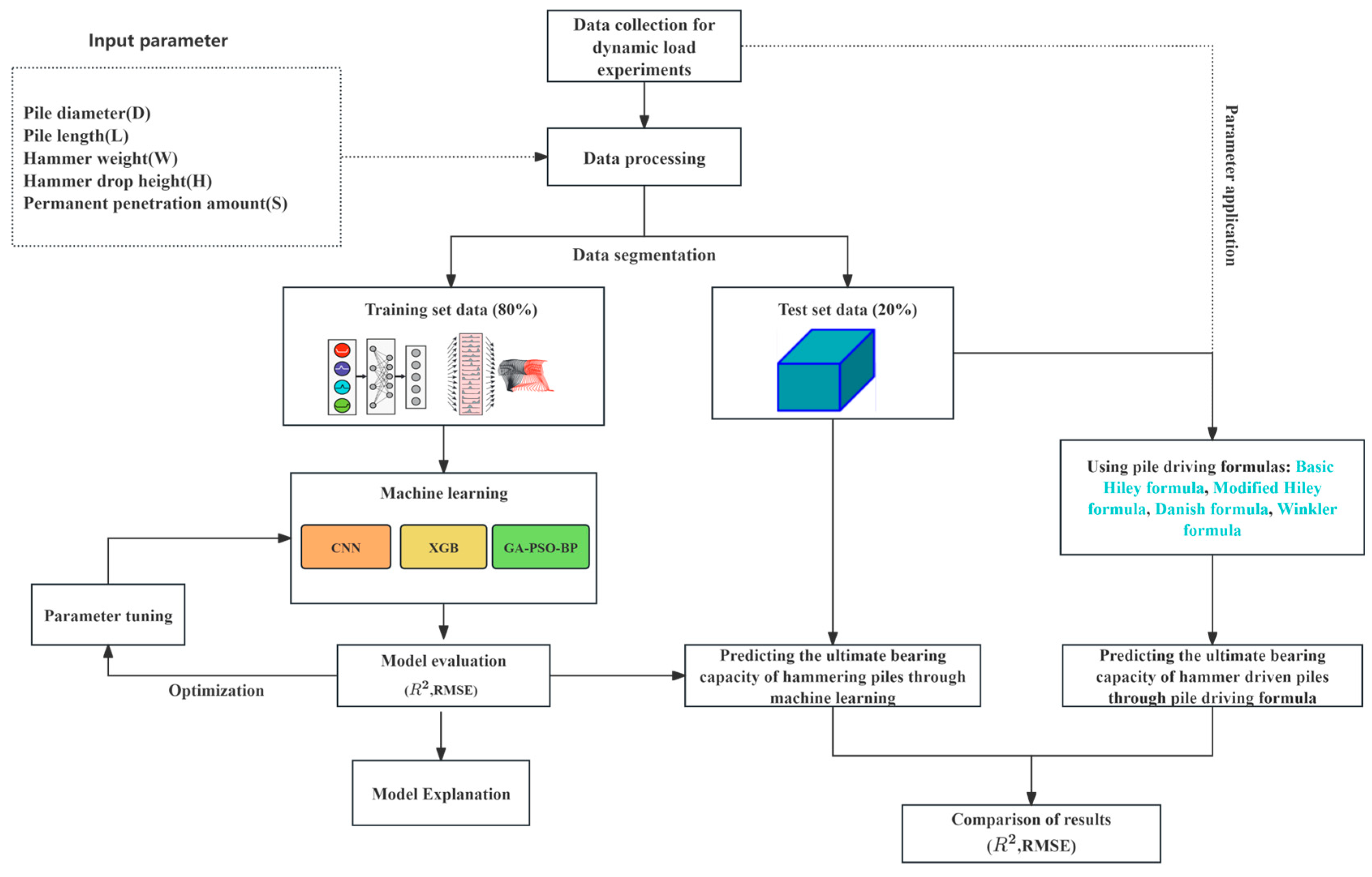
The complete workflow of this study is depicted in Figure 2. It begins with the collection of raw data from dynamic load testing on hammer-driven piles. After preprocessing steps including normalization, outlier handling, and feature engineering, the dataset is divided into training and testing sets at an 8:2 ratio. Three modeling approaches are employed: Convolutional Neural Network (CNN), which captures spatial hierarchies and local dependencies; Extreme Gradient Boosting (XGB), known for its strong capability in learning complex patterns and resistance to overfitting; and Backpropagation Neural Network (BPNN), which, despite its powerful nonlinear fitting ability, is prone to falling into local optima. To overcome this limitation, a hybrid GA–PSO–BPNN model is proposed, integrating Genetic Algorithm (GA) and Particle Swarm Optimization (PSO) to combine global search capabilities with efficient convergence, thereby improving prediction accuracy and stability. The hybrid model is compared with CNN, XGB, traditional dynamic formulas (including Hiley, Danish, Winkler, and their modified versions), and actual measurement data to demonstrate the superiority of the machine learning approach. Additionally, SHAP value analysis is employed to interpret the influence of input variables, and the model’s applicability is discussed in light of the distinct characteristics of pre-drilled and precast piles. This integrated methodology combines machine learning with traditional techniques, enabling a comprehensive evaluation of UBC. The integration of GA and PSO is motivated by their complementary strengths: GA enhances global exploration through crossover and mutation to avoid premature convergence, whereas PSO provides rapid local exploitation by refining candidate solutions with adaptive inertia weights. Their combination allows the GA–PSO–BPNN framework to balance exploration and exploitation, resulting in more robust and accurate optimization outcomes than GA-BPNN or PSO-BPNN alone.

The GA-PSO-BPNN model developed in this study is designed for use with a specific range of input parameters and pile types. The model was trained on data derived from high-strain dynamic testing (PDA) of hammer-driven piles, which includes input variables such as pile diameter (D), hammer weight (W), hammer drop height (H), permanent penetration (S), and pile length (L). The model’s predictions are most accurate within the ranges of these input variables, which were defined based on the dataset used for training.

However, caution is advised when applying the model to situations beyond the defined input ranges. For example, extrapolation to pile types other than hammer-driven piles (e.g., bored piles, continuous flight auger piles) or geotechnical conditions that differ significantly from those represented in the dataset may lead to inaccurate predictions. Additionally, the model does not account for factors such as groundwater level, soil heterogeneity, and extreme environmental conditions, which can significantly affect the ultimate bearing capacity (UBC) but were not included in the training data. Thus, the model’s predictions should be limited to the scope of use defined by the current dataset, and users should avoid extrapolation to conditions outside this domain.

3. Data Preparation and Experimental Configuration

3.1. Data Preparation

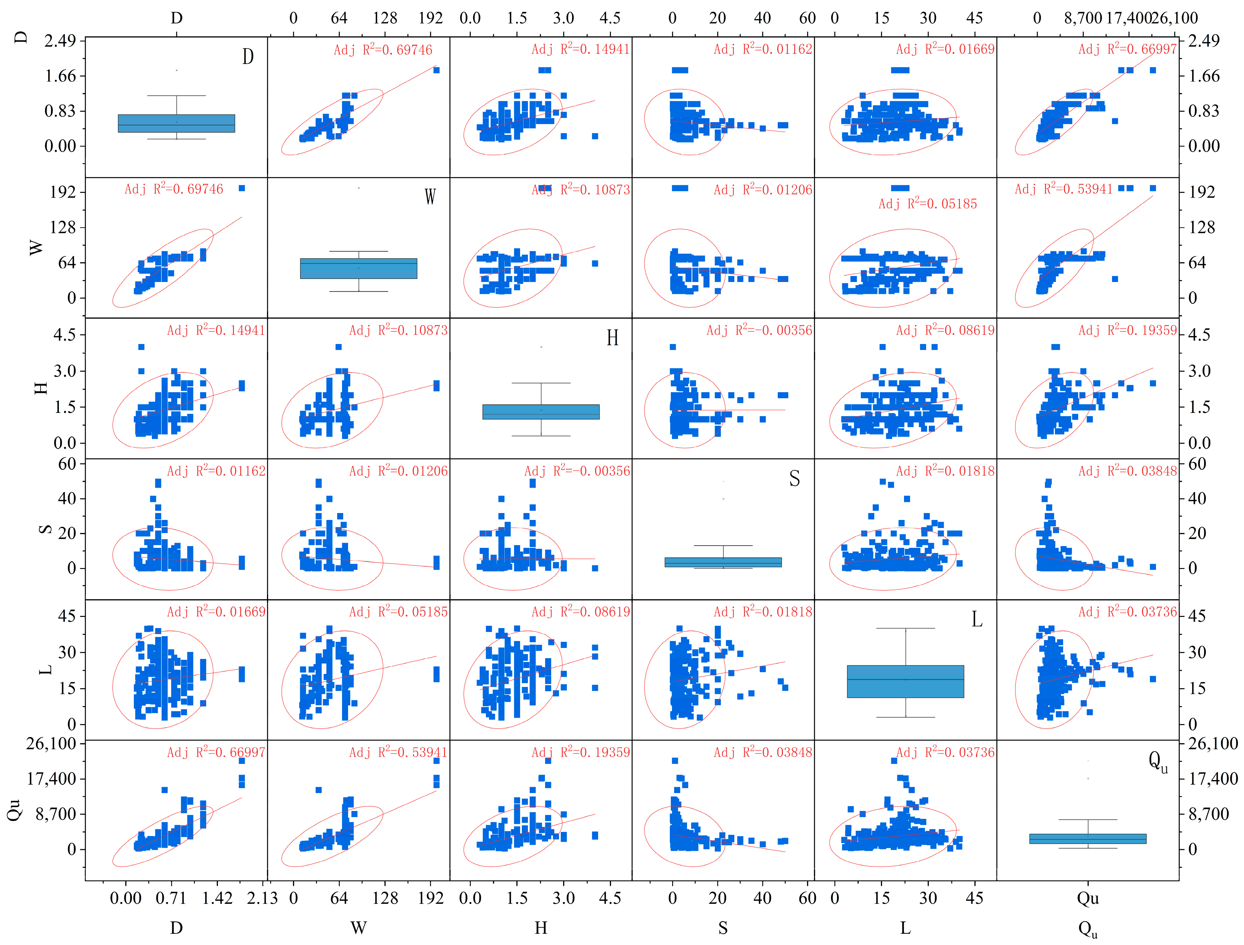
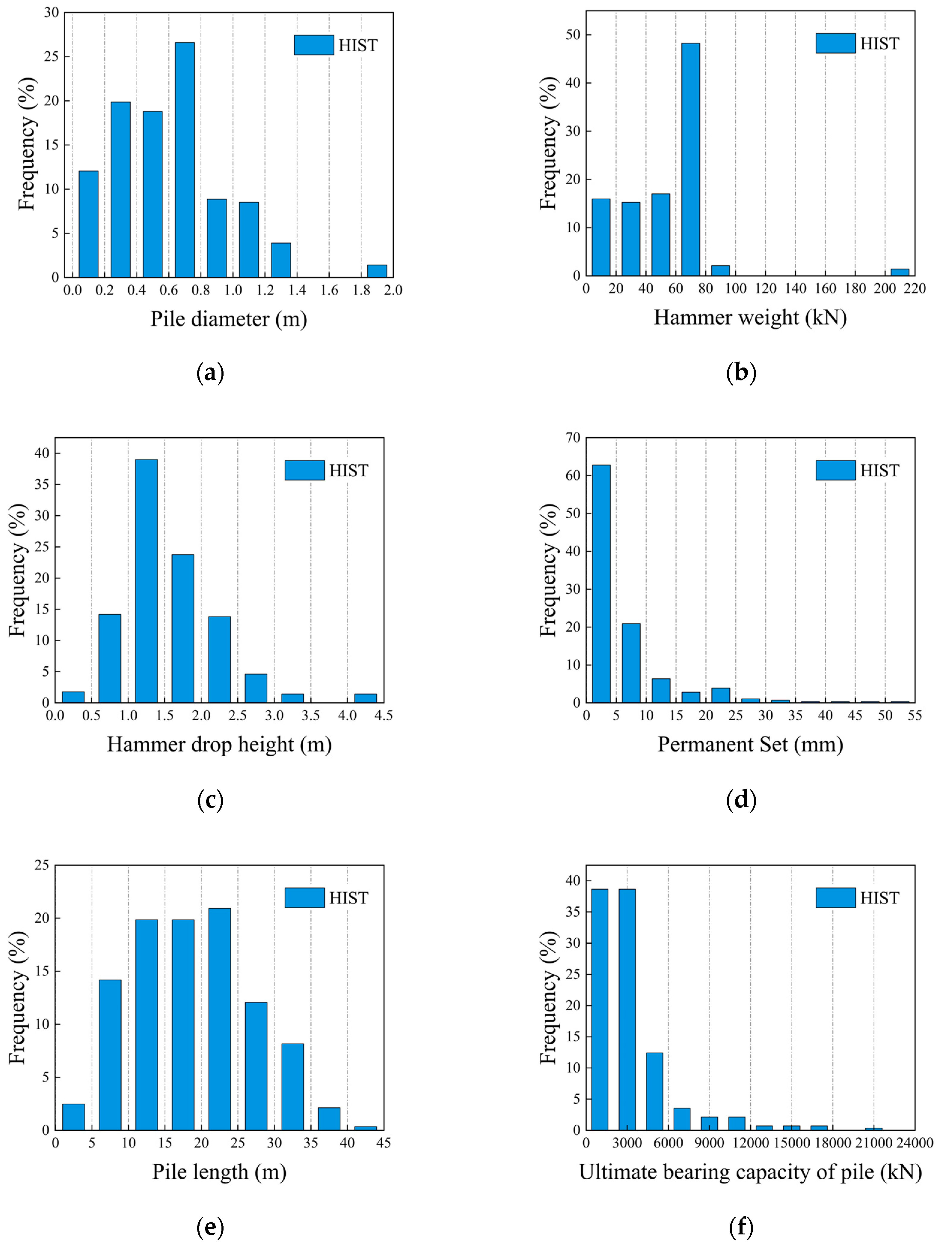
The dataset used in this study is primarily derived from two key sources: Pessoa et al. [48] and Momeni et al. [49], which provide comprehensive high-strain dynamic testing (PDA) data across a wide range of pile types, construction methods, and geological conditions. These datasets offer a robust foundation for model development, ensuring diversity and reliability through their extensive geographical and technical coverage. Figure 3 presents a scatter matrix of variable relationships, with Pearson correlation coefficients (expressed as adjusted $R^2$ values) displayed below the diagonal and box plots illustrating variable distributions above it. The analysis reveals notably high correlations between diameter (D) and Ultimate bearing capacity of pile ($Q_u$), as well as hammer weight (W) and Ultimate bearing capacity of pile ($Q_u$), necessitating careful examination of these variables in subsequent modeling to mitigate potential multicollinearity and overfitting. In contrast, height (H), S, and length (L) exhibit weak correlations with other variables, indicating a low risk of multicollinearity. Overall, the generally low correlations among most independent variables suggest that the model inputs maintain satisfactory independence. The corresponding variable distributions are shown in Figure 4. The histograms indicate that hammer drop height is primarily distributed between 0.5 and 1.5 m, with a distinct peak at around 1 m. Hammer weight values are concentrated near 60 kN, reflecting standard practice in field testing. Permanent penetration values are heavily skewed toward the 0–5 mm range, indicating that minimal residual settlement is most common. Pile diameters are relatively evenly distributed, with frequent occurrences between 0.6 and 0.8 m. Pile lengths exhibit a mild right-skewed trend, with the majority falling in the 20–30 m range. The ultimate bearing capacity ($Q_u$) shows a concentration around 3000 kN, with fewer instances of higher values. Skewness analysis confirms that most variables exhibit near-symmetric distributions, suggesting a balanced dataset suitable for machine learning applications.

3.2. Data Preprocessing

This study uses a dataset obtained from dynamic load tests performed on key construction projects in Brazil and Sri Lanka. The dataset was split into training and testing sets using an 80:20 ratio, with a fixed random seed of 3,659,418,059 to ensure reproducibility. Additionally, the data split was stratified by site (Brazil and Sri Lanka) to maintain representative proportions of samples from each site in both the training and testing sets. During preprocessing, input variables were normalized to the range [0, 1] via Min-Max scaling, while extreme values were identified and either removed or adjusted using the Interquartile Range (IQR) method, with a total of 14 records removed or adjusted across all variables. After outlier handling, the final dataset contained 282 records. To mitigate overfitting risks and enhance generalization, 10-fold cross-validation was performed strictly within the training partition, ensuring that no test data leakage occurred during the model development and evaluation phases. Hyperparameter tuning was also conducted exclusively on the training data. These measures helped ensure the reliability of the results and the robustness of the model.

For the XGBoost model, the optimal configuration n = 300, learning rate = 0.001, and max depth = 10—achieved an effective bias–variance trade-off, resulting in the highest $R^2$ value. In the CNN model, given its sensitivity to batch size and learning rate, the Adam optimizer was adopted with a batch size of 10, and mean squared error (MSE) was used as the metric to systematically evaluate the impact of network depth on performance. The GA-PSO-BPNN model determined the optimal number of hidden neurons through empirical formulas and root mean squared error (RMSE), with the best R² attained using a population size of 450, cognitive and social coefficients set to $C_1$ = 2.286 and $C_2$ = 1.714, and a genetic operation size of 25. The final hyperparameter configurations for all models are summarized in

Table 2. The control parameters and optimized hyperparameters for the CNN, XGB, and GA-PSO-BPNN models.

Model	XGB	CNN	GA-PSO-BPNN
Control parameter	n_estimators = 300 learning_rate = 0.001 max_depth = 10	Input Layer Shape: [32, 1, 5, 1] Convolutional Layer Filters: 32, Kernel size: [10, 1] Pooling Layer Pool size: [1, 10], Stride: 10 Adam optimizer, Learning rate: 0.004	population size = 450 ${\mathrm{C}}_1$ = 2.286, ${\mathrm{C}}_2$ = 1.714 genetic operation size = 25

, providing a reproducible and robust experimental foundation for predicting the UBC foundations.

3.3. Performance Metrics

The predictive performance of the models was comprehensively evaluated using four key metrics: the coefficient of determination ($R^2$), root mean square error (RMSE), mean absolute error (MAE), and mean absolute percentage error (MAPE). $R^2$ quantified the proportion of variance explained by the model, while RMSE and MAE provided absolute measures of prediction error, with RMSE being more sensitive to larger deviations. MAPE complemented these by expressing error in relative terms, offering an intuitive assessment of prediction accuracy as a percentage.

$${\mathrm{R}}^2=1-{\displaystyle \frac{\sum _{\mathrm{i}=1}^{\mathrm{n}}\left({\mathrm{y}}_{\mathrm{i}}-{\widehat{\mathrm{y}}}_{\mathrm{i}}\right)}{\sum _{\mathrm{i}=1}^{\mathrm{n}}\left({\mathrm{y}}_{\mathrm{i}}-{\overline{\mathrm{y}}}_{\mathrm{i}}\right)}}$$

(1)

$$\mathrm{R}\mathrm{M}\mathrm{S}\mathrm{E}=\sqrt{{\displaystyle \frac{1}{\mathrm{n}}}\sum _{\mathrm{i}=1}^{\mathrm{n}}{\left({\mathrm{y}}_{\mathrm{i}}-{\widehat{\mathrm{y}}}_{\mathrm{i}}\right)}^2}$$

(2)

$$\mathrm{M}\mathrm{A}\mathrm{E}={\displaystyle \frac{1}{\mathrm{n}}}\sum _{\mathrm{i}=1}^{\mathrm{n}}\left|{\mathrm{y}}_{\mathrm{i}}-{\widehat{\mathrm{y}}}_{\mathrm{i}}\right|$$

(3)

$$\mathrm{M}\mathrm{A}\mathrm{P}\mathrm{E}=\sum _{\mathrm{i}=1}^{\mathrm{n}}\left|{\displaystyle \frac{{\mathrm{y}}_{\mathrm{i}}-{\widehat{\mathrm{y}}}_{\mathrm{i}}}{{\mathrm{y}}_{\mathrm{i}}}}\right|\cdot {\displaystyle \frac{1}{\mathrm{n}}}$$

(4)

Here, ${\mathrm{y}}_{\mathrm{i}}$ denotes the observed values, ${\widehat{y}}_{\mathrm{i}}$ the predicted values, and ${\overline{y}}_i$ the mean of the observed data. The coefficient of determination ($R^2$) quantifies the proportion of variance explained by the model, RMSE measures the square root of average squared errors with stronger penalties for larger deviations, MAE captures the average magnitude of errors regardless of direction, and MAPE expresses errors as a percentage of actual values, facilitating relative comparisons across models.

3.4. Explanatory Approach

In machine learning, SHAP (SHapley Additive exPlanations) values are employed to quantify the contribution of individual input features to model predictions. Rooted in cooperative game theory, SHAP allocates feature importance based on the concept of Shapley values, offering a model-agnostic framework for interpreting output decisions in a mathematically grounded and consistent manner. By evaluating all possible subsets of features, the method computes the average marginal contribution of each feature across all permutations, ensuring a fair distribution of influence among predictors. A positive SHAP value signifies that the feature increases the predicted output, whereas a negative value indicates a suppressing effect. This approach enhances transparency in black-box models by identifying critical features and clarifying local decision mechanisms, thereby facilitating model diagnostics and validation. Antwarg et al. [50] emphasized that SHAP outperforms alternative interpretation techniques such as LIME in terms of consistency, robustness, and usability. Owing to its compatibility with diverse model architectures—including CNNs, XGBoost, and hybrid systems like GA-PSO-BPNN used in this study—SHAP provides a unified and scalable tool for evaluating feature importance across a wide range of machine learning models.

4. Results

4.1. Comparison of Performance Among AI-Based Prediction Models

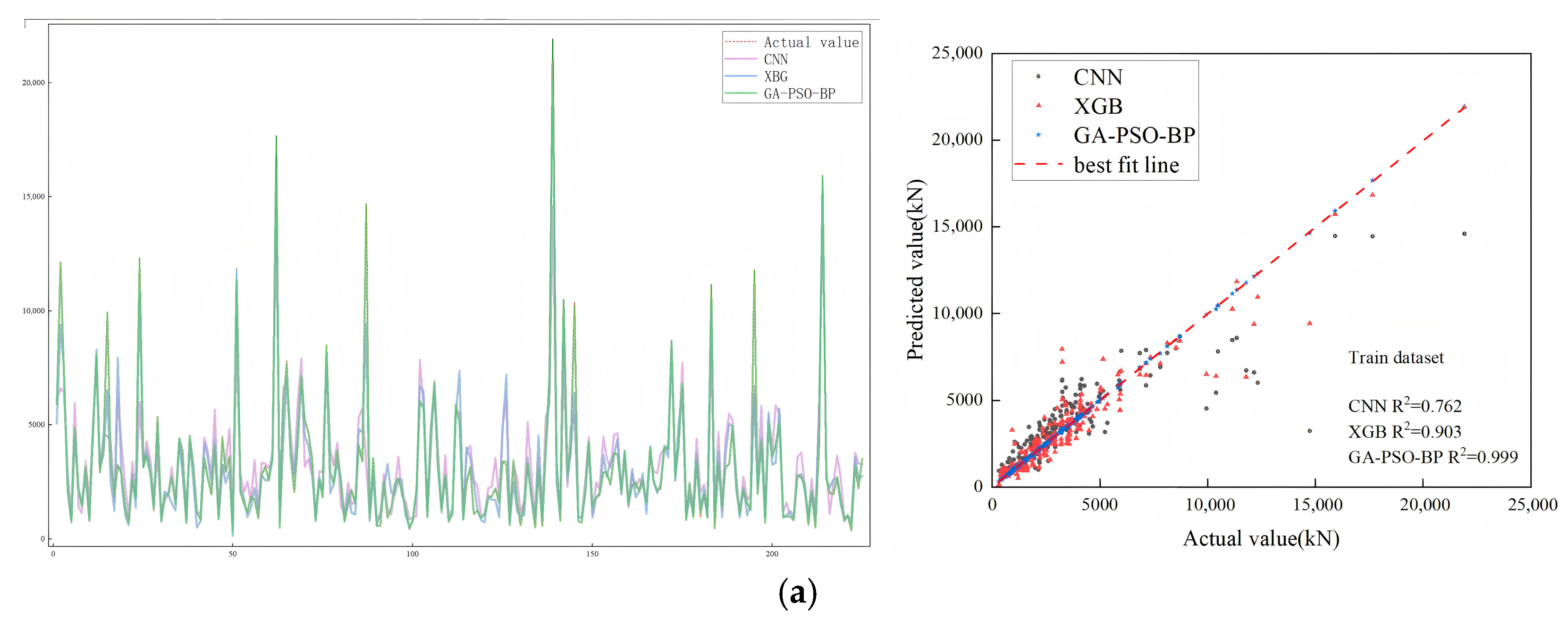
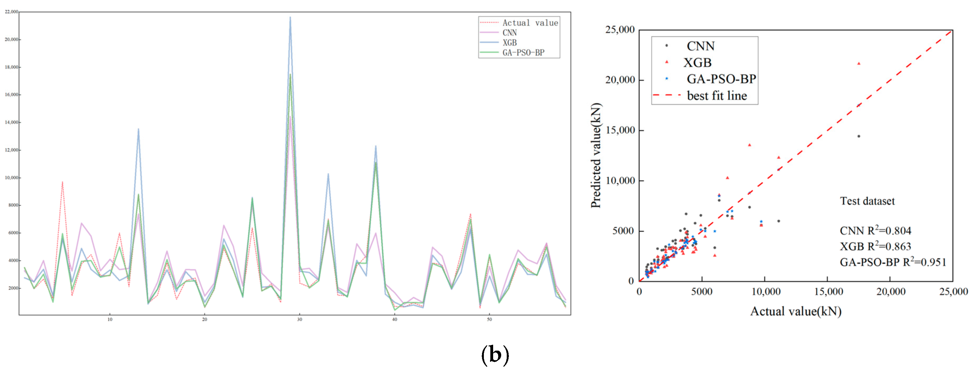
In this work, three machine learning models—CNN, XGB, and GA-PSO-BPNN—were applied to predict UBC driving. Their performance was assessed using both training and testing datasets, with the outcomes summarized in Figure 5 and

Table 3. Results of UBC prediction performance using CNN, XGB, and GA-PSO-BPNN.

Model	${\mathbf{R}}^2$		MAPE		RMSE		MAE
	TR	TE	TR	TE	TR	TE	TR	TE
CNN	0.762	0.804	0.325	0.381	1520.31	1390.90	867.72	998.94
XGB	0.903	0.863	0.210	0.239	945.87	1350.07	521.52	836.15
GA-PSO-BPNN	0.999	0.951	0.013	0.135	39.28	660.13	27.41	328.51

. As shown in Figure 5, the predicted values from all three models generally match the measured results (CAPWAP) well. The scatter plots indicate that predictions near the best-fit line correspond to higher accuracy. Among the tested models, GA-PSO-BPNN achieved the best performance, with an ${\mathrm{R}}^2$ value of 0.999, followed by XGB and CNN. For the testing dataset, the scatter plots also confirm GA-PSO-BPNN as the most accurate, yielding the highest ${\mathrm{R}}^2$ value of 0.951, ahead of XGB and CNN.

Table 3 displays the performance metrics for both the training and testing datasets, offering a detailed analysis of the predictive capabilities of each machine learning model. The GA-PSO-BPNN model shows excellent performance on the training data, with a MAPE of 1.33%, RMSE of 39.28, and MAE of 27.41, indicating high accuracy. However, on the test data, despite a slight increase in MAPE and RMSE, the GA-PSO-BPNN model maintains relatively low values of MAPE (13.46%), RMSE (660.13), and MAE (328.51), demonstrating superior generalization capability compared to both CNN and XGBoost. In contrast, the CNN model exhibits an MAPE of 32.52%, RMSE of 1520.31, and MAE of 867.72 on the training data, with MAPE increasing further to 38.05% on the test data, which indicates considerable overfitting. The XGBoost model performs with a MAPE of 21.03%, RMSE of 945.87, and MAE of 521.52 on the training data, and on the test data, the MAPE is 23.97%, RMSE is 1350.07, and MAE is 836.15. Although the performance is comparatively stable, there remains a significant gap compared to the GA-PSO-BPNN model. Overall, the GA-PSO-BPNN model demonstrates strong generalization ability and lower error metrics, making it highly suitable for predicting the ultimate bearing capacity of impact-driven piles.

4.2. Analysis of Variable Significance in AI-Based Prediction Models

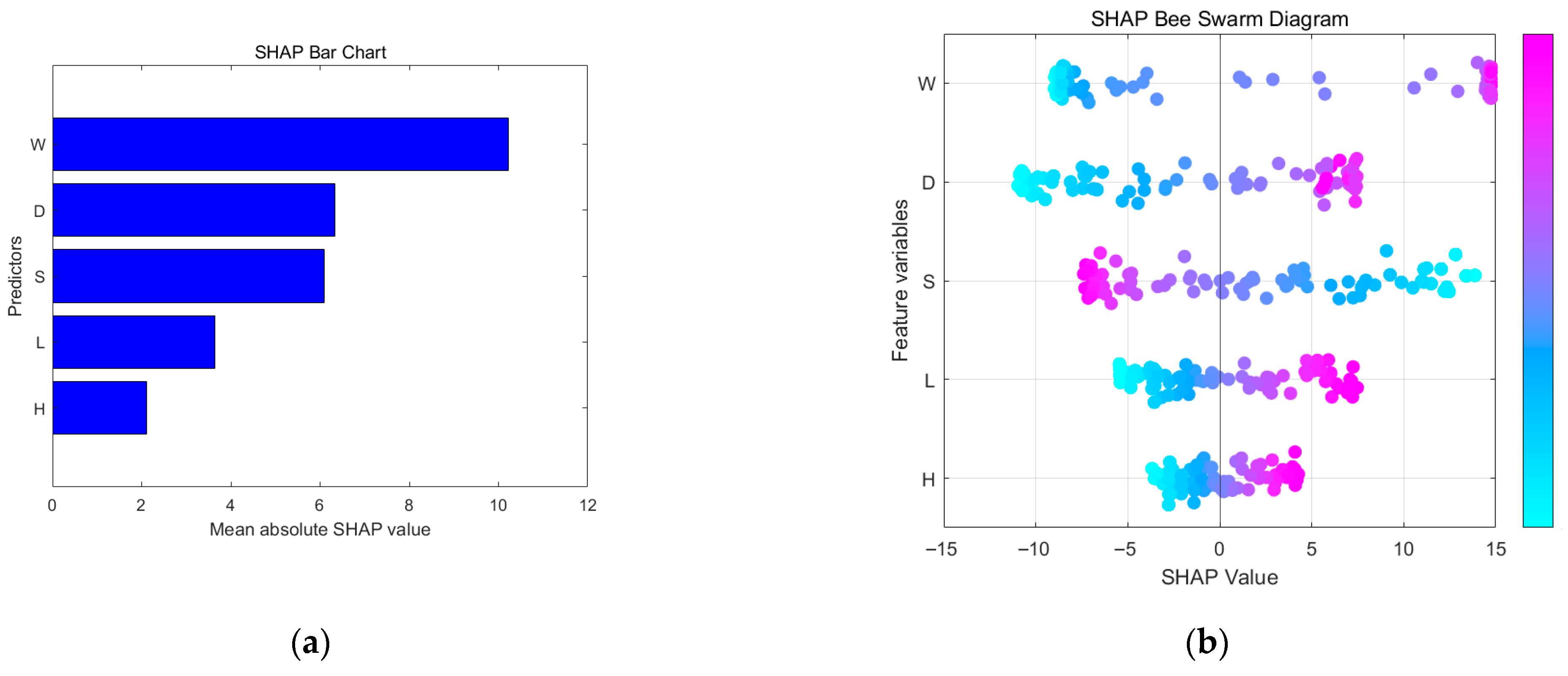
In this study, the sensitivity of the established GA-PSO-BPNN model Figure 6 was analyzed by using the shap algorithm, and the influence of input parameters on the prediction of pile foundation bearing capacity was quantified by a bee colony diagram and bar graph. The shap bar graph shows that the average absolute shap value of the hammer weight W (kN) is the highest (close to 10), indicating that its contribution to the model output is the most significant. The shap value of W in the bee colony diagram is concentrated in the positive range (5–15), indicating that increasing the hammer weight can significantly improve the predicted value of pile foundation bearing capacity, which is consistent with the mechanism of high-energy penetration of heavy hammer to enhance pile-soil densification in practical engineering. The low sensitivity of H conforms to the “energy dominated” theory in pile foundation dynamics, that is, the bearing capacity is mainly determined by the hammering energy (W × H), but w has dominated the energy representation in the model, resulting in the weakening of the independent contribution of H. This result is consistent with the engineering experience of the “heavy hammer low impact” process in the literature [51], which further verifies the rationality of the model.

In this study, the sensitivity of the GA-PSO-BPNN model (Figure 6) was analyzed using the SHAP algorithm, and the influence of input parameters on the prediction of pile foundation bearing capacity was quantified using a beeswarm plot and bar graph. The SHAP bar graph indicates that the average absolute SHAP value for W (hammer weight) is the highest (close to 10), suggesting that its contribution to the model’s output is the most significant. The SHAP values for W in the beeswarm plot are concentrated in the positive range (5–15), showing that an increase in hammer weight significantly enhances the predicted pile foundation bearing capacity. This finding aligns with the physical mechanism of high-energy penetration by a heavy hammer, which promotes pile-soil densification in practical engineering.

The complete global ranking based ”n SH’P values is as follows: W (hammer weight) > D (diameter) > S (permanent set) > L (length) > H (hammer drop height). The low sensitivity of H supports the “energy-dominated” theory in pile foundation dynamics, where bearing capacity is primarily determined by hammering energy (W × H). However, in this model, W (hammer weight) becomes the dominant factor, overshadowing the independent contribution of H (hammer drop height), as the model places greater emphasis on the hammer weight in determining pile bearing capacity.

D (diameter), which affects the pile’s contact area with the surrounding soil, is ranked second, reflecting its role in load distribution and bearing capacity. S (permanent set), which measures the pile’s residual deformation after hammering, is ranked third, indicating its influence on densification and load resistance. L (length) is ranked fourth, showing its contribution to the depth of pile penetration and stability, though its impact is less significant compared to W and D. Finally, H (hammer drop height), while still a contributing factor, ranks the lowest, emphasizing its secondary role in pile capacity compared to hammer weight and diameter.

This result is consistent with the “heavy hammer, low impact” process described in the literature [51], further validating the model’s rationale.

4.3. The Variable Importance Analysis of Prediction Models Based on Artificial Intelligence

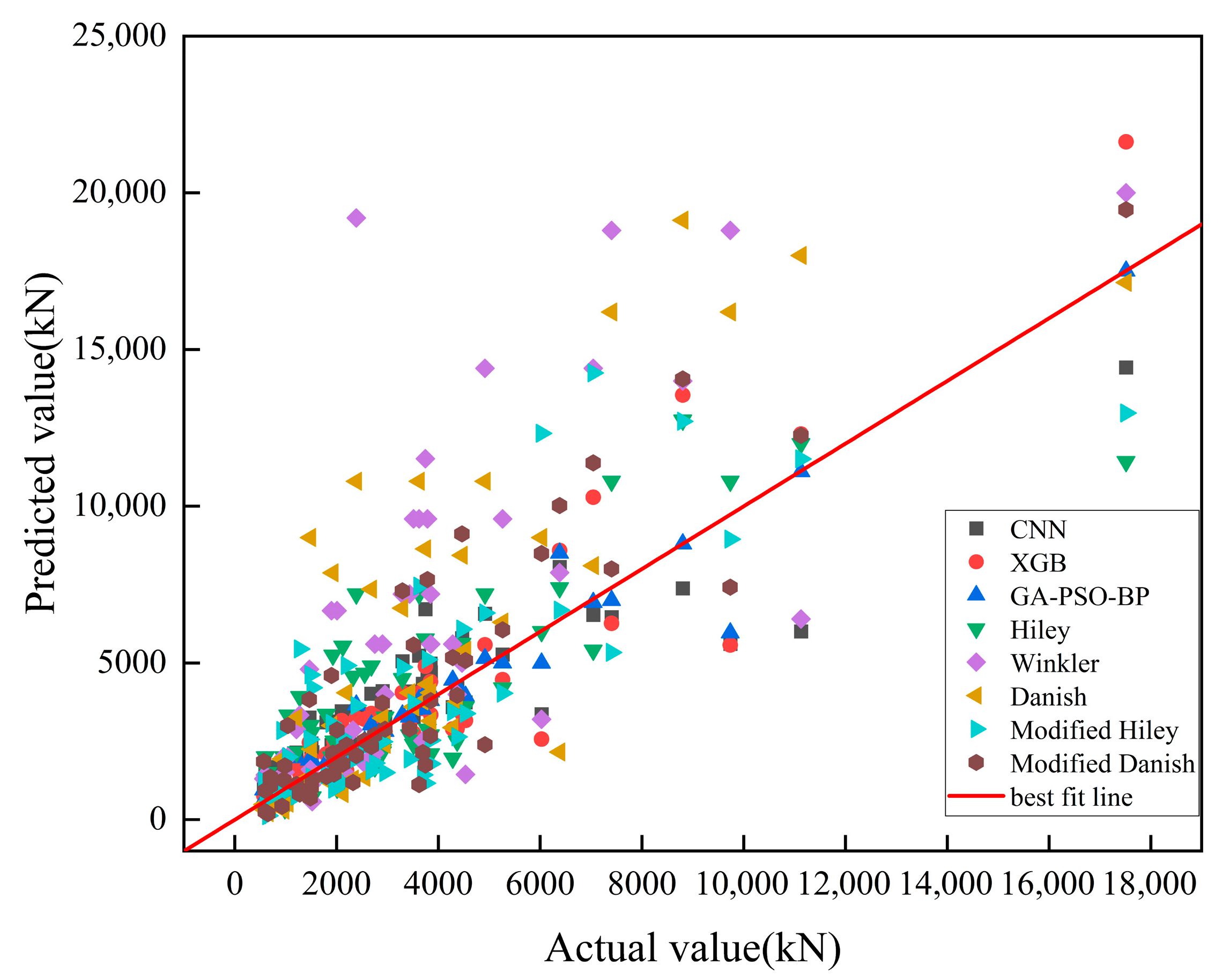
Figure 7 presents a comparison between three AI models (CNN, XGB, and GA-PSO-BPNN) and traditional dynamic piling formulas (Hiley, Winkler, Danish, etc.) in predicting the UBC. As shown in the figure, the predictions made by the AI models align closely with the best-fit line, indicating a significant advantage in terms of prediction accuracy. Specifically, the GA-PSO-BPNN model exhibits the highest predictive capability with an $R^2$ value of 0.951. Furthermore, its error metrics (such as MAPE, RMSE, and MAE) are notably lower than those of the other models, demonstrating its ability to more accurately capture the variations in UBC. In contrast, traditional dynamic piling formulas, such as the Winkler and Danish formulas, have $R^2$ values of −0.863 and −0.286, respectively, reflecting poor predictive performance and leading to substantial prediction errors. These formulas tend to either overestimate or underestimate the UBC, with the Winkler formula exhibiting particularly large prediction errors. Although the modified Hiley and Danish formulas show some improvement, their $R^2$ values remain lower than those of the AI models, suggesting limited capability in handling complex nonlinear relationships. The performance metrics in

Table 4. The use of neural networks and empirical formulas in predicting UBCs.

Model	${\mathit{R}}^2$	MAPE	RMSE	MAE
CNN	0.804	0.381	1390.9	998.49
XGB	0.863	0.239	1350.07	836.15
GA-PSO-BPNN	0.951	0.135	660.13	328.51
Hiley	0.588	0.615	1890.48	1460.69
Winkler	−0.863	0.901	4240.56	2748.28
Danish	−0.286	0.681	3342.23	2043.95
Modified Hiley	0.515	0.523	2051.78	1415.28
Modified Danish	0.638	0.456	1773.24	1211.08

further corroborate this observation: both the GA-PSO-BPNN and XGB models have high $R^2$ values and low error metrics, highlighting the superiority of AI models in capturing complex relationships and enhancing prediction accuracy. While the modified traditional formulas show some improvement when dynamic load testing energy values are introduced, their accuracy still falls short compared to the AI models, particularly in scenarios involving higher ultimate pile bearing capacities.

5. Discussion

This study introduces a novel hybrid model, GA-PSO-BPNN, for predicting the ultimate bearing capacity (UBC) of driven piles. The results show that the GA-PSO-BPNN model outperforms traditional methods and other machine learning models, including CNN and XGB, with an R² value of 0.951 and an RMSE of 660.13. These results confirm the model’s high accuracy and generalizability across different soil types and pile configurations, highlighting the potential of hybrid machine learning approaches for addressing the complexities in pile capacity prediction in geotechnical engineering.

The findings of this study are in agreement with previous research, which has demonstrated the effectiveness of machine learning models in predicting pile-bearing capacity. Alwalan and El Naggar [3] used analytical models based on dynamic tests to predict pile responses and observed similar improvements in prediction accuracy. However, unlike their approach, which relied on simplified assumptions about soil conditions, our model incorporates a broader set of input features and utilizes advanced optimization algorithms (GA and PSO) to improve model performance. This allows for a more accurate representation of the complex, nonlinear relationships between pile capacity and geotechnical parameters.

In contrast to the study by Yin et al. [2], which focused on dynamic damage around pile tips, our approach leverages a data-driven methodology, using large-scale datasets and machine learning techniques to analyze pile behavior. This shift towards data-driven modeling reduces the reliance on idealized assumptions, making our model more adaptable to real-world scenarios. Additionally, while Zhang and Xue [5] developed hybrid models for end-bearing capacity prediction in rock-socketed piles, our GA-PSO-BPNN model improves upon their work by combining the strengths of both GA and PSO, which enhances optimization robustness and parameter space exploration.

A key innovation of this study is the integration of GA and PSO with BPNN for predicting pile UBC. Previous studies have used individual machine learning algorithms, but the hybridization of GA, PSO, and BPNN provides a more effective solution to geotechnical prediction challenges. The combination of GA and PSO enhances the global search and optimization capabilities, making the model more efficient and reliable. This hybrid approach not only improves prediction accuracy but also increases the model’s adaptability to various soil conditions and pile configurations, overcoming the limitations of earlier models.

Moreover, this study contributes to the growing trend of integrating optimization techniques with machine learning models, as seen in recent works by Pham et al. [21] and Kumar et al. [22]. By combining optimization algorithms with machine learning, the proposed model offers a more robust solution for solving complex, nonlinear problems in geotechnical engineering, providing a promising approach for future advancements in pile foundation design.

The GA-PSO-BPNN model can be integrated into routine design practices, offering significant advantages in terms of cost, ease of deployment, and maintenance. While the model requires more computational resources for training and prediction compared to traditional methods, the increasing computational power, particularly with the rise in cloud computing and big data platforms, is expected to reduce the application costs over time. Optimizing the algorithms and leveraging hardware acceleration can further improve training and prediction efficiency, thus reducing operational costs in the long term. Although the model’s structure is relatively complex, it can be integrated into engineering practice by simplifying input/output processes and developing user-friendly interfaces. By incorporating the model into existing design tools, engineers can easily input parameters (such as pile diameter, length, and hammer weight) and obtain predictions without needing to understand the underlying machine learning mechanisms. Given that the model is based on machine learning, its performance may vary with new construction data and different geological conditions; therefore, regular updates are recommended to maintain prediction accuracy. Automating the process of data updates and model retraining will reduce the need for manual intervention, making maintenance more efficient. In future work, we plan to optimize the model’s computational efficiency by exploring lightweight algorithms or model compression techniques to reduce its cost in routine design applications. Additionally, by incorporating real-time feedback from field testing and continuous data updates, the model will improve over time, allowing it to accommodate a broader range of application scenarios.

6. Conclusions

This study demonstrates the potential of AI-based models for predicting the ultimate bearing capacity (UBC) of driven piles, with the proposed GA-PSO-BPNN framework achieving high accuracy (R² = 0.999 for training and R² = 0.951 for testing). By integrating Genetic Algorithm (GA) and Particle Swarm Optimization (PSO), the hybrid model addresses limitations of conventional BPNN, such as local optima and premature convergence, and shows superior adaptability to complex pile-soil interactions compared to traditional dynamic formulas. Furthermore, SHAP analysis improves interpretability by highlighting the influence of key input parameters, including pile diameter, hammer weight, and permanent penetration.

These findings emphasize the advantages of AI-driven approaches as reliable and transparent alternatives to traditional predictive methods. However, it should be noted that the current framework does not incorporate advanced principles such as plastic analysis or reliability-based design. Future research will seek to address these gaps by integrating plastic and shakedown responses, deformation control, and the consideration of uncertainties in material properties, manufacturing processes, and geometric variations. Furthermore, the inclusion of additional geotechnical parameters—such as soil classification, layer thickness, and groundwater conditions—will further improve the accuracy and generalizability of the model.

By combining AI-driven predictions with reliability-based design principles, future research will offer a more comprehensive approach to pile foundation design, ensuring not only structural strength but also consistent long-term performance in diverse geotechnical conditions.

References

1. Meyerhof, G.G.; Asce, F. Bearing Capacity and Settlement of Pile Foundations. J. Geotech. Eng. Div. ASCE 1976, 102, 197–228. [Google Scholar] [CrossRef]
2. Yin, J.; Bai, X.; Yan, N.; Sang, S.; Cui, L.; Liu, J.; Zhang, M. Dynamic Damage Characteristics of Mudstone around Hammer Driven Pile and Evaluation of Pile Bearing Capacity. Soil Dyn. Earthq. Eng. 2023, 167, 107789. [Google Scholar] [CrossRef]
3. Alwalan, M.F.; El Naggar, M.H. Analytical Models of Impact Force-Time Response Generated from High Strain Dynamic Load Test on Driven and Helical Piles. Comput. Geotech. 2020, 128, 103834. [Google Scholar] [CrossRef]
4. Alkroosh, I.; Nikraz, H. Predicting Pile Dynamic Capacity via Application of an Evolutionary Algorithm. Soils Found. 2014, 54, 233–242. [Google Scholar] [CrossRef]
5. Zhang, R.; Xue, X. A Novel Hybrid Model for Predicting the End-bearing Capacity of Rock-socketed Piles. Rock Mech. Rock Eng. 2024, 57, 10099–10114. [Google Scholar] [CrossRef]
6. Maizir, H.; Suryanita, R.; Jingga, H. Estimation of Pile Bearing Capacity of Single Driven Pile in Sandy Soil Using Finite Element and Artificial Neural Network Methods. Int. J. Appl. Phys. Sci. 2016, 2, 50002–50003. [Google Scholar] [CrossRef]
7. Kordjazi, A.; Pooya Nejad, F.; Jaksa, M.B. Prediction of Ultimate Axial Load-Carrying Capacity of Piles Using a Support Vector Machine Based on CPT Data. Comput. Geotech. 2014, 55, 91–102. [Google Scholar] [CrossRef]
8. Alkroosh, I.S.; Bahadori, M.; Nikraz, H.; Bahadori, A. Regressive Approach for Predicting Bearing Capacity of Bored Piles from Cone Penetration Test Data. J. Rock Mech. Geotech. Eng. 2015, 7, 584–592. [Google Scholar] [CrossRef]
9. Jahed Armaghani, D.; Shoib, R.S.N.S.B.R.; Faizi, K.; Rashid, A.S.A. Developing a Hybrid PSO–ANN Model for Estimating the Ultimate Bearing Capacity of Rock-Socketed Piles. Neural Comput. Appl. 2017, 28, 391–405. [Google Scholar] [CrossRef]
10. Wang, B.; Moayedi, H.; Nguyen, H.; Foong, L.K.; Rashid, A.S.A. Feasibility of a Novel Predictive Technique Based on Artificial Neural Network Optimized with Particle Swarm Optimization Estimating Pullout Bearing Capacity of Helical Piles. Eng. Comput. 2020, 36, 1315–1324. [Google Scholar] [CrossRef]
11. Armaghani, D.J.; Harandizadeh, H.; Momeni, E.; Maizir, H.; Zhou, J. An Optimized System of GMDH-ANFIS Predictive Model by ICA for Estimating Pile Bearing Capacity. Artif. Intell. Rev. 2022, 55, 2313–2350. [Google Scholar] [CrossRef]
12. Yong, W. A New Hybrid Simulated Annealing-Based Genetic Programming Technique to Predict the Ultimate Bearing Capacity of Piles. Eng. Comput. 2021, 37, 2111–2127. [Google Scholar] [CrossRef]
13. Prayogo, D.; Susanto, Y.T.T. Optimizing the Prediction Accuracy of Friction Capacity of Driven Piles in Cohesive Soil Using a Novel Self-Tuning Least Squares Support Vector Machine. Adv. Civ. Eng. 2018, 2018, 6490169. [Google Scholar] [CrossRef]
14. Borthakur, N.; Dey, A.K. Evaluation of Group Capacity of Micropile in Soft Clayey Soil from Experimental Analysis Using SVM-Based Prediction Model. Int. J. Geomech. 2020, 20, 04020008. [Google Scholar] [CrossRef]
15. Harandizadeh, H.; Toufigh, M.M.; Toufigh, V. Application of Improved ANFIS Approaches to Estimate Bearing Capacity of Piles. Soft Comput. 2019, 23, 9537–9549. [Google Scholar] [CrossRef]
16. Harandizadeh, H.; Jahed Armaghani, D.; Khari, M. A New Development of ANFIS–GMDH Optimized by PSO to Predict Pile Bearing Capacity Based on Experimental Datasets. Eng. Comput. 2021, 37, 685–700. [Google Scholar] [CrossRef]
17. Dehghanbanadaki, A.; Khari, M.; Amiri, S.T.; Armaghani, D.J. Estimation of Ultimate Bearing Capacity of Driven Piles in C-φ Soil Using MLP-GWO and ANFIS-GWO Models: A Comparative Study. Soft Comput. 2021, 25, 4103–4119. [Google Scholar] [CrossRef]
18. Momeni, E.; Dowlatshahi, M.B.; Omidinasab, F.; Maizir, H.; Armaghani, D.J. Gaussian Process Regression Technique to Estimate the Pile Bearing Capacity. Arab. J. Sci. Eng. 2020, 45, 8255–8267. [Google Scholar] [CrossRef]
19. Momeni, E.; Nazir, R.; Jahed Armaghani, D.; Maizir, H. Application of Artificial Neural Network for Predicting Shaft and Tip Resistances of Concrete Piles. Earth Sci. Res. J. 2015, 19, 85–93. [Google Scholar] [CrossRef]
20. Moayedi, H.; Moatamediyan, A.; Nguyen, H.; Bui, X.-N.; Bui, D.T.; Rashid, A.S.A. Prediction of Ultimate Bearing Capacity through Various Novel Evolutionary and Neural Network Models. Eng. Comput. 2020, 36, 671–687. [Google Scholar] [CrossRef]
21. Pham, T.A.; Tran, V.Q.; Vu, H.-L.T.; Ly, H.-B. Design Deep Neural Network Architecture Using a Genetic Algorithm for Estimation of Pile Bearing Capacity. PLoS ONE 2020, 15, e0243030. [Google Scholar] [CrossRef] [PubMed]
22. Kumar, M.; Kumar, D.R.; Khatti, J.; Samui, P.; Grover, K.S. Prediction of Bearing Capacity of Pile Foundation Using Deep Learning Approaches. Front. Struct. Civ. Eng. 2024, 18, 870–886. [Google Scholar] [CrossRef]
23. Pham, T.A.; Ly, H.-B.; Tran, V.Q.; Giap, L.V.; Vu, H.-L.T.; Duong, H.-A.T. Prediction of Pile Axial Bearing Capacity Using Artificial Neural Network and Random Forest. Appl. Sci. 2020, 10, 1871. [Google Scholar] [CrossRef]
24. Yaychi, B.M.; Esmaeili-Falak, M. Estimating Axial Bearing Capacity of Driven Piles Using Tuned Random Forest Frameworks. Geotech. Geol. Eng. 2024, 42, 7813–7834. [Google Scholar] [CrossRef]
25. Amjad, M.; Ahmad, I.; Ahmad, M.; Wróblewski, P.; Kamiński, P.; Amjad, U. Prediction of Pile Bearing Capacity Using XGBoost Algorithm: Modeling and Performance Evaluation. Appl. Sci. 2022, 12, 2126. [Google Scholar] [CrossRef]
26. Esmaeili-Falak, M.; Benemaran, R.S. Ensemble Extreme Gradient Boosting Based Models to Predict the Bearing Capacity of Micropile Group. Appl. Ocean Res. 2024, 151, 104149. [Google Scholar] [CrossRef]
27. Nguyen, H.; Cao, M.-T.; Tran, X.-L.; Tran, T.-H.; Hoang, N.-D. A Novel Whale Optimization Algorithm Optimized XGBoost Regression for Estimating Bearing Capacity of Concrete Piles. Neural Comput. Appl. 2023, 35, 3825–3852. [Google Scholar] [CrossRef]
28. Moayedi, H.; Jahed Armaghani, D. Optimizing an ANN Model with ICA for Estimating Bearing Capacity of Driven Pile in Cohesionless Soil. Eng. Comput. 2018, 34, 347–356. [Google Scholar] [CrossRef]
29. Yago, G.; Verri, F.; Ribeiro, D. Use of Machine Learning Techniques for Predicting the Bearing Capacity of Piles. Soils Rocks 2021, 44, e2021074921. [Google Scholar] [CrossRef]
30. Kardani, N.; Zhou, A.; Nazem, M.; Shen, S.-L. Estimation of Bearing Capacity of Piles in Cohesionless Soil Using Optimised Machine Learning Approaches. Geotech. Geol. Eng. 2020, 38, 2271–2291. [Google Scholar] [CrossRef]
31. Zhou, T. Developing a Machine Learning-Driven Model That Leverages Meta-Heuristic Algorithms to Forecast the Load-Bearing Capacity of Piles. J. Artif. Intell. Syst. Model. 2023, 1, 1–14. [Google Scholar] [CrossRef]
32. Liu, Q.; Cao, Y.; Wang, C. Prediction of Ultimate Axial Load-Carrying Capacity for Driven Piles Using Machine Learning Methods. In Proceedings of the 2019 IEEE 3rd Information Technology, Networking, Electronic and Automation Control Conference (ITNEC), Chengdu, China, 15–17 March 2019. [Google Scholar]
33. Yousheng, D.; Keqin, Z.; Zhongju, F.; Wen, Z.; Xinjun, Z.; Huiling, Z. Machine Learning Based Prediction Model for the Pile Bearing Capacity of Saline Soils in Cold Regions. Structures 2024, 59, 105735. [Google Scholar] [CrossRef]
34. Dadhich, S.; Sharma, J.K.; Madhira, M. Prediction of Ultimate Bearing Capacity of Aggregate Pier Reinforced Clay Using Machine Learning. Int. J. Geosynth. Ground Eng. 2021, 7, 44. [Google Scholar] [CrossRef]
35. Sun, Z.; Liu, F.; Han, Y.; Min, R. Prediction of Ultimate Bearing Capacity of Rock-Socketed Piles Based on GWO-SVR Algorithm. Structures 2024, 61, 106039. [Google Scholar] [CrossRef]
36. Cao, Y.; Ni, J.; Chen, J.; Geng, Y. Rapid Evaluation Method to Vertical Bearing Capacity of Pile Group Foundation Based on Machine Learning. Sensors 2025, 25, 1214. [Google Scholar] [CrossRef] [PubMed]
37. Zhang, W.; Li, H.; Li, Y.; Liu, H.; Chen, Y.; Ding, X. Application of Deep Learning Algorithms in Geotechnical Engineering: A Short Critical Review. Artif. Intell. Rev. 2021, 54, 5633–5673. [Google Scholar] [CrossRef]
38. Karakaş, S.; Taşkın, G.; Ülker, M.B.C. Re-Evaluation of Machine Learning Models for Predicting Ultimate Bearing Capacity of Piles through SHAP and Joint Shapley Methods. Neural Comput. Appl. 2024, 36, 697–715. [Google Scholar] [CrossRef]
39. Ouyang, W.; Li, G.; Chen, L.; Liu, S.-W. Machine Learning-Based Soil–Structure Interaction Analysis of Laterally Loaded Piles through Physics-Informed Neural Networks. Acta Geotech. 2024, 19, 4765–4790. [Google Scholar] [CrossRef]
40. Abdulkadirov, R.; Lyakhov, P.; Nagornov, N. Survey of Optimization Algorithms in Modern Neural Networks. Mathematics 2023, 11, 2466. [Google Scholar] [CrossRef]
41. Rausche, F.; Moses, F.; Goble, G.G. Soil resistance predictions from pile dynamics. J. Soil Mech. Found. Div. 1972, 98, 917–937. [Google Scholar] [CrossRef]
42. Rausche, F.; Goble, G.G.; Likins, G.E., Jr. Dynamic determination of pile capacity. J. Geotech. Eng. 1985, 111, 367–383. [Google Scholar] [CrossRef]
43. Hannigan, P.J.; Goble, G.G.; Thendean, G.; Likins, G.E.; Rausche, F. Design and Construction of Driven Pile Foundations—Volume I (Report No. FHWA-HI-97-013); Federal Highway Administration: Washington, DC, USA, 1998. Available online: https://rosap.ntl.bts.gov/view/dot/58200 (accessed on 20 October 2025).
44. ASTM D4945; Standard Test Method for High-Strain Dynamic Testing of Piles. ASTM International: West Conshohocken, PA, USA, 1989.
45. EN ISO 22476-1; Geotechnical Investigation and Testing—Field Testing—Part 1: Electrical Resistivity and High-Strain Dynamic Testing of Piles. International Organization for Standardization (ISO): Geneva, Switzerland, 2012.
46. Paikowsky, S.G.; Hart, L.J. Development and Field Testing of Multiple Deployment Model Pile (MDMP) (Report No. FHWA-RD-99-194); Federal Highway Administration: Washington, DC, USA, 2000. Available online: https://highways.dot.gov/sites/fhwa.dot.gov/files/FHWA-RD-99-194.pdf (accessed on 20 October 2025).
47. Prakash, S.; Sharma, H.D. Pile Foundations in Engineering Practice; John Wiley & Sons: Hoboken, NJ, USA, 1991. [Google Scholar]
48. Pessoa, A.D.; Sousa, G.C.L.D.; Araujo, R.D.C.D.; Anjos, G.J.M.D. Artificial Neural Network Model for Predicting Load Capacity of Driven Piles. Res. Soc. Dev. 2021, 10, e12210111526. [Google Scholar] [CrossRef]
49. Momeni, E.; Nazir, R.; Jahed Armaghani, D.; Maizir, H. Prediction of Pile Bearing Capacity Using a Hybrid Genetic Algorithm-Based ANN. Measurement 2014, 57, 122–131. [Google Scholar] [CrossRef]
50. Antwarg, L.; Miller, R.M.; Shapira, B.; Rokach, L. Explaining Anomalies Detected by Autoencoders Using Shapley Additive Explanations. Expert Syst. Appl. 2021, 186, 115736. [Google Scholar] [CrossRef]
51. Wang, J.-C.; Yu, J.; Shiguo, M.; Gong, X. Hammer’s Impact Force on Pile and Pile’s Penetration. Mar. Georesour. Geotechnol. 2016, 34, 409–419. [Google Scholar] [CrossRef]
Figure 1. Ultimate bearing capacity measurement of single pile via PDA.
Buildings 15 03839 g001
Figure 2. Procedure for developing the UBC prediction model.
Buildings 15 03839 g002
Figure 3. Scatter matrix diagram of variable relationships.
Buildings 15 03839 g003
Figure 4. Graphical illustration using a histogram (HIST) of surveying data: (a) input X 1 —Pile diameter (D); (b) input X 2 —Hammer weight (W); (c) input X 3 —Hammer drop height (H); (d) input X 4 —Permanent Set (S); (e) input X 5 —Pile length (L); (f) output Y—Ultimate bearing capacity of pile ( Q u ).
Buildings 15 03839 g004
Figure 5. The prediction outcomes of AI models across driving stages for both training and testing datasets. (a) training datasets; (b) test datasets.
Buildings 15 03839 g005aBuildings 15 03839 g005b
Figure 6. Explanation of driving phase prediction model using SHAP (a) SHAP Bar Chart, (b) SHAP Bee Swarm.
Buildings 15 03839 g006
Figure 7. AI models and dynamic driving formulas for predicting the results of the test dataset.
Buildings 15 03839 g007