Article

Machine Learning-Based Rapid Assessment of Story-Level Seismic Damage in Steel Bundled-Tube Structures

1
School of Civil and Engineering, Hebei University of Architecture, Zhangjiakou 075000, China
2
School of Information Engineering, Hebei University of Architecture, Zhangjiakou 075000, China
3
Hebei Key Laboratory of Diagnosis, Reconstruction and Anti-Disaster of Civil Engineering, Zhangjiakou 075000, China
*
Author to whom correspondence should be addressed.
Buildings 2025, 15(20), 3758; https://doi.org/10.3390/buildings15203758
Submission received: 8 September 2025 / Revised: 2 October 2025 / Accepted: 16 October 2025 / Published: 17 October 2025
(This article belongs to the Section Building Structures)

Abstract

This study employed machine learning to establish an intelligent model for rapid and accurate seismic damage assessment of steel bundled-tube stories. The study built a 100-story elastoplastic steel bundled-tube model based on an actual engineering case, and then extracted and labeled data. Eight machine learning algorithms were employed to assess the seismic damage states of the steel bundled-tube stories. Hyperparameter optimization was performed on the two best-performing algorithms, and Shapley Additive Explanations (SHAP) analysis was used to investigate the influence of input variables on the five damage states. Using original parameters, Random Forest (RF) and Extreme Gradient Boosting (XGBoost) showed highest accuracies (94.6% and 94.3%). After optimization, XGBoost’s accuracy rose by 2.2% to 96.5%, outperforming RF, and is thus recommended as the final model. This study fills the gap in story-level damage assessment using machine learning. SHAP analysis revealed peak acceleration and story load-bearing capacity as core variables. Displacement is more crucial in the low-damage state, while energy dissipation plays a dominant role in the high-damage state, which poses a challenge to the traditional seismic design that only limits displacement. The method identifies weak stories for targeted reinforcement, optimizing seismic performance of steel bundled-tube structures.

1. Introduction

The traditional Chinese seismic design principle, which stipulates “no damage under minor earthquakes, repairable under moderate earthquakes, and no collapse under major earthquakes,” prioritizes human safety during an earthquake but overlooks post-earthquake damage assessment and reconstruction efforts [1,2,3,4]. In the current post-earthquake assessment process, experts perform visual inspections of affected sites individually and then evaluate the damage to buildings based on their expertise [5,6,7,8]. This manual evaluation depends heavily on extensive experience and demands considerable time for on-site investigations [9,10,11,12]. Machine learning-based damage assessment offers clear advantages, enabling swift and precise evaluation of damage states using established databases [13,14,15,16]. Recently, advancements in machine learning algorithms and the emergence of artificial intelligence have increasingly positioned this approach as a prominent focus in building structure damage assessment research [17,18,19,20,21]. Research on damage assessment can be categorized into three areas based on the research objects: overall structural damage assessment, story-level damage assessment, and component-level damage assessment. Extensive research on the overall structural damage assessment using machine learning has been conducted by various authors. He et al. [22] introduced a hybrid deep learning method for damage identification, utilizing Ensemble Empirical Mode Decomposition, Pearson Correlation Coefficient (PCC), and Convolutional Neural Network (CNN), and demonstrated its feasibility on a three-story frame structure. Bhatta and Dang [23] developed simulated datasets to predict seismic damage states in RC buildings, training models and validating their performance with real data from the 2015 Nepal earthquake. Nguyen et al. [24] created eight models for assessing damage states in steel moment frames, selecting the RF model for its superior performance and developing a user interface. Wang [25] compiled a database of reinforced concrete structures and employed RF algorithm to propose a multivariate feature-based prediction method for seismic damage. Extensive research has been conducted on applying machine learning to component damage. Ni and Duan [26] developed a shear test database of 200 UHPFRC beams and proposed three machine learning models—Artificial Neural Network (ANN), support vector regression (SVR), and XGBoost—to calculate shear strength. Zhao et al. [27] utilized ten parameters related to reinforced concrete slabs and explosions to predict maximum displacement under blast loads, demonstrating high predictive performance of the machine learning model. Naderpour et al. [28] applied Decision Tree (DT) and neural networks to forecast failure modes of reinforced concrete columns, finding that DT offer high accuracy without complex calculations. Sujith Mangalathu et al. [29] evaluated eight machine learning models and introduced an RF-based model to predict failure modes of reinforced concrete shear walls, achieving an 86% accuracy in identifying failure modes. Furthermore, the integration of machine learning with mechanical principles has shown promising results in predicting the structural response of advanced systems, such as self-centering structures [30]. This demonstrates the potential of hybrid machine learning -mechanics models not only for damage classification but also for response prediction, providing a comprehensive analytical framework. Numerous studies have explored machine learning applications for assessing damage in overall structures and components. However, in-depth research on using machine learning to assess the damage state of stories is still lacking.
The present study employed machine learning algorithms to assess seismic damage of steel bundled-tube structural stories. An elastoplastic model of the steel bundled-tube was developed, and seismic waves were applied. Relevant data were extracted, labeled, and compiled into a comprehensive database. Eight machine learning algorithms, including DT, RF, k-Nearest Neighbors (KNN), Support Vector Machine (SVM), Naive Bayes (NB), XGBoost, Adaptive Boosting (Adaboost), and Categorical Boosting (CatBoost), were utilized to assess seismic damage of steel bundled-tube stories. The study rigorously compared the performance of different machine learning models. Hyperparameter optimization was carried out on the top two performing algorithms, RF and XGBoost, out of the eight models evaluated. Subsequently, SHAP were utilized to clarify the impact of input variables on the five damage states. This study fills the gap in story-level damage assessment using machine learning, provides reference value for subsequent damage assessment based on machine learning, and offers new ideas for practical engineering applications.

2. Steel Bundled-Tube Story-Level Damage Dataset

2.1. Establishment of the Steel Bundled-Tube Model

In this study, a 100-story steel bundled-tube structure with a floor height of 3.6 m each is established based on an actual engineering case, and the structural height is 360 m. The entire steel bundled-tube is composed of nine 22.5 m × 22.5 m frame tube structures. The single-story plane is a square with dimensions of 67.5 m × 67.5 m, and the column spacing is 4.5 m. The steel components are fabricated from Q420 grade steel. The reinforced concrete floor slab uses C30 grade concrete and HRB400 grade reinforcing bars, with a thickness of 110 mm and reinforced in a two-way pattern with 8-mm-diameter HRB400 bars at 200-mm spacing. Table 1 provides detailed dimensions of all structural components.
This study employs ABAQUS (version 2022) finite element analysis software to develop an elastoplastic model of the steel bundled-tube, depicted in Figure 1. The model utilizes B31 linear beam elements for the beams and columns, and S4R two-dimensional shell elements for the floor slabs. In compliance with the “Code for Seismic Design of Buildings” (GB 50011-2010) [31], three seismic waves are chosen: two natural waves, HWA043 and TTN024, and one artificial wave, R. The ground motion duration is set at 40 s, utilizing bidirectional input. This ratio of 1:0.85 between principal and secondary directional peak accelerations is mandated by Clause 5.1.5 of the Chinese Code for Seismic Design of Buildings (GB 50011-2010) for bidirectional time-history analysis. It reflects the code-specified intensity proportion for input ground motions in nonlinear dynamic analysis.

2.2. Verification of Model Accuracy

To verify the model’s accuracy, the steel bundled-tube was modeled using PKPM software (version 2025). Modal analysis was performed with both PKPM and ABAQUS. The first three modal periods and the total structural mass were compared. Table 2 presents the comparison results, revealing that the first three-order periods and total structural mass calculated by PKPM and ABAQUS are closely aligned, with a maximum discrepancy of less than 1%. This indicates that the finite element model of the steel bundled-tube developed in this study is reasonably accurate.

2.3. Assessment of Story-Level Damage States

The damage states of steel bundled-tube stories in the database were assessed using plastic-strain-based criteria developed by our research group [32]. This choice is motivated by three key reasons: firstly, plastic strain is a direct field output from our ABAQUS finite element models, offering an unambiguous measure of material nonlinearity. Secondly, it is fundamentally related to the physical mechanism of damage, as plastic hinge rotation is geometrically linked to the integration of plastic strain over a critical length. Lastly, these criteria provide a pragmatic and consistent basis for translating continuous simulation data into discrete damage states across various structural components. Table 3 details the established criteria for these damage state.
The first step is to determine the damage state of steel members based on the corresponding relationship between the damage degree of steel members and the unit plastic strain in Table 4. Then, it will be determined the overall damage degree of the story by statistically analyzing the damage conditions of steel members.
According to Table 3, The story damage factor D0 can be comprehensively determined according to the proportion of the damage degree of the steel columns, steel beams and floor steel bars in the story among the same type of components in that story. On a particular floor, 10.7% of steel columns are undamaged, 16.5% are slightly damaged, 71.4% are in obvious damage zone I, and 1.3% are in obvious damage zone II. Additionally, 35.3% of steel skirt beams are undamaged, 52.2% are slightly damaged, and 12.5% are in obvious damage zone I. Furthermore, 26.1% of floor slab reinforcement is undamaged, 71.9% is slightly damaged, and 2% is in obvious damage zone I. The calculation process of the story damage factor D0 on this story is shown in Formula (1). According to Table 5, which correlates damage factors with damage states, the story damage story D0 of 0.594 indicates moderate damage for the story.
D0 = 0.065 + 0.370 + 0.020 + 0.060 + 0.040 + 0.035 + 0.004 = 0.594

2.4. Construction of the Dataset

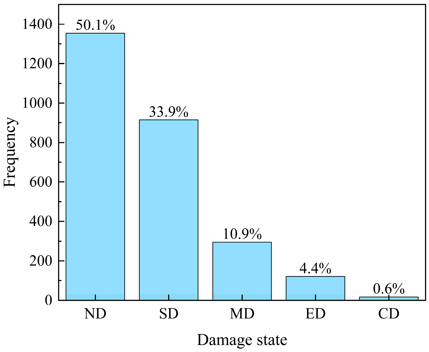
To enhance the dataset’s data volume and the comprehensiveness of damage data for each state, peak seismic accelerations for the steel bundled-tube elastoplastic model were chosen as 220 Gal, 400 Gal, 620 Gal, 1800 Gal, 2000 Gal, 2500 Gal, 3000 Gal, 3500 Gal, and 4000 Gal. 27 elastoplastic time-history analyses were performed on a 100-story steel bundled-tube model, yielding 2700 damage data points for the steel bundled-tube stories. Subsequently, a dataset was established for the machine learning model through data extraction and processing. Based on the assessment criteria outlined in Section 2.3 regarding damage phenomena, seismic damage states for steel bundled-tube stories are categorized into five groups: no damage (ND), slight damage (SD), moderate damage (MD), extensive damage (ED), and complete collapse (CD). The distribution of seismic damage states among 2700 steel bundled-tube stories is depicted in Figure 2, indicating that 1354 stories (50.1%) experienced no damage, 914 stories (33.9%) were slightly damaged, 295 stories (10.9%) were moderately damaged, 120 stories (4.4%) were extensively damaged, and 17 stories (0.6%) were completely collapsed.
The precise selection of input parameters is essential to enhance the accuracy of the prediction model. These parameters, necessary for evaluating the damage state, can be categorized into three main parts: building information features, earthquake information features, and structural response features. This study examines building information features, which encompass basic structural details and resistance to external forces. It also examines earthquake information features, which indicate the magnitude of ground motion intensity. Finally, it examines structural response features, which detail the dynamic response induced by ground motion. These three features encompass the basic information of the building stories before the earthquake, the ground motion intensity during the earthquake, and the final structural response after the earthquake. All parameters play a crucial role in the assessment of the damage state.
This paper focuses on assessing damage to steel bundled-tube stories. Therefore, priority is given to selecting parameters related to the story information. Low-rise stories are typically vulnerable floors prone to damage, while high-rise stories often experience significant damage due to acceleration amplification. Hence, the number of floors is chosen as an input variable when considering building information features. Mass is a fundamental parameter influencing inertia. A higher story mass results in increased inertial forces, thereby elevating the risk of structural damage. Therefore, story mass is chosen as an input variable. Abrupt alterations in story stiffness can cause stress concentration within the structure, with stiffness being interconnected with the structure’s natural vibration period. Consequently, story stiffness is chosen as another input variable. The bearing capacity directly correlates with the ability to withstand ground motion. Insufficient bearing capacity compared to seismic internal forces can lead to structural damage or collapse. Therefore, the story load-bearing capacity is selected. Peak acceleration is a key parameter in seismic data selection, indicating ground motion intensity and influencing the inertial forces on structures. Although PGA is an input intensity measure and PFA a resultant structural response—linked through the structure’s dynamic characteristics such as mode shapes and nonlinear behavior—this study employs PGA as the input feature. This decision is based on its role as the most direct and generalizable design parameter for seismic intensity, enabling quick access and straightforward application in practical engineering scenarios. This study prioritizes story-level seismic response parameters for damage assessment. While global-level indices such as base shear and base moment are critically important, they are excluded here. This is because they represent the integrated structure-ground motion response, necessitating indirect derivation through numerical modeling. Such derivation relies on extensive specialized data, making these parameters often prohibitively difficult to acquire. Hence, parameters like base shear and base moment were not selected. Displacement serves as a clear indicator of structural damage when choosing structural response features. Various regulations such as China’s “Code for Seismic Design of Buildings,” “Technical Specification for Concrete Structures of Tall Buildings,” and the United States’ “IBC” emphasize the importance of limiting displacement to ensure structural safety and viability. Energy consumption directly correlates with the accumulation of damage, prompting several countries to shift towards energy-based seismic structural design approaches. This metric serves as a direct output from finite element software, providing a comprehensive reflection of nonlinear behavior and damage accumulation at the story level. For instance, the United States’ “FEMA Seismic Risk Assessment Methodology” introduces an energy-based method for assessing seismic performance. Consequently, story energy consumption and maximum story displacement are ultimately chosen as the primary structural response features.
This paper initially identifies seven parameters as input variables for machine learning. These variables encompass building information features, earthquake information features, and structural response features. The building information features comprise floor number (F), story mass (m), story stiffness (K), and story load-bearing capacity (C). The earthquake information features consist of peak acceleration (a), while the structural response features include story energy consumption (E) and maximum story displacement (x). The seismic damage state of the steel bundled-tube story is designated as the output variable.
The building information features are extracted from the computational outcomes of the PKPM software. The floor number comprises between 1 and 100 floors. The story mass is the aggregate of the masses induced by the dead and live loads. The story stiffness is derived from the stiffness in the x-direction, while the story load-bearing capacity is based on the load-bearing capacity in the x-direction. Given the structural symmetry of the building and the predominant earthquake force along the x-direction, both the story stiffness and load-bearing capacity are established with reference to the x-direction. The peak acceleration of the earthquake information feature is determined by the maximum absolute value of the input seismic wave’s acceleration, categorized into 220 Gal, 400 Gal, 620 Gal, 1800 Gal, 2000 Gal, 2500 Gal, 3000 Gal, 3500 Gal, and 4000 Gal. The structural response features are derived from the ABAQUS elastoplastic time-history analysis model. Story energy consumption represents the total plastic energy dissipation of the story during an earthquake. The maximum story displacement is determined as the highest value obtained from the displacements in both the X and Y directions of each control point (the four corner points located at the top of the story). Table 6 gives the corresponding value ranges for each input parameter.

2.5. Optimization of the Dataset

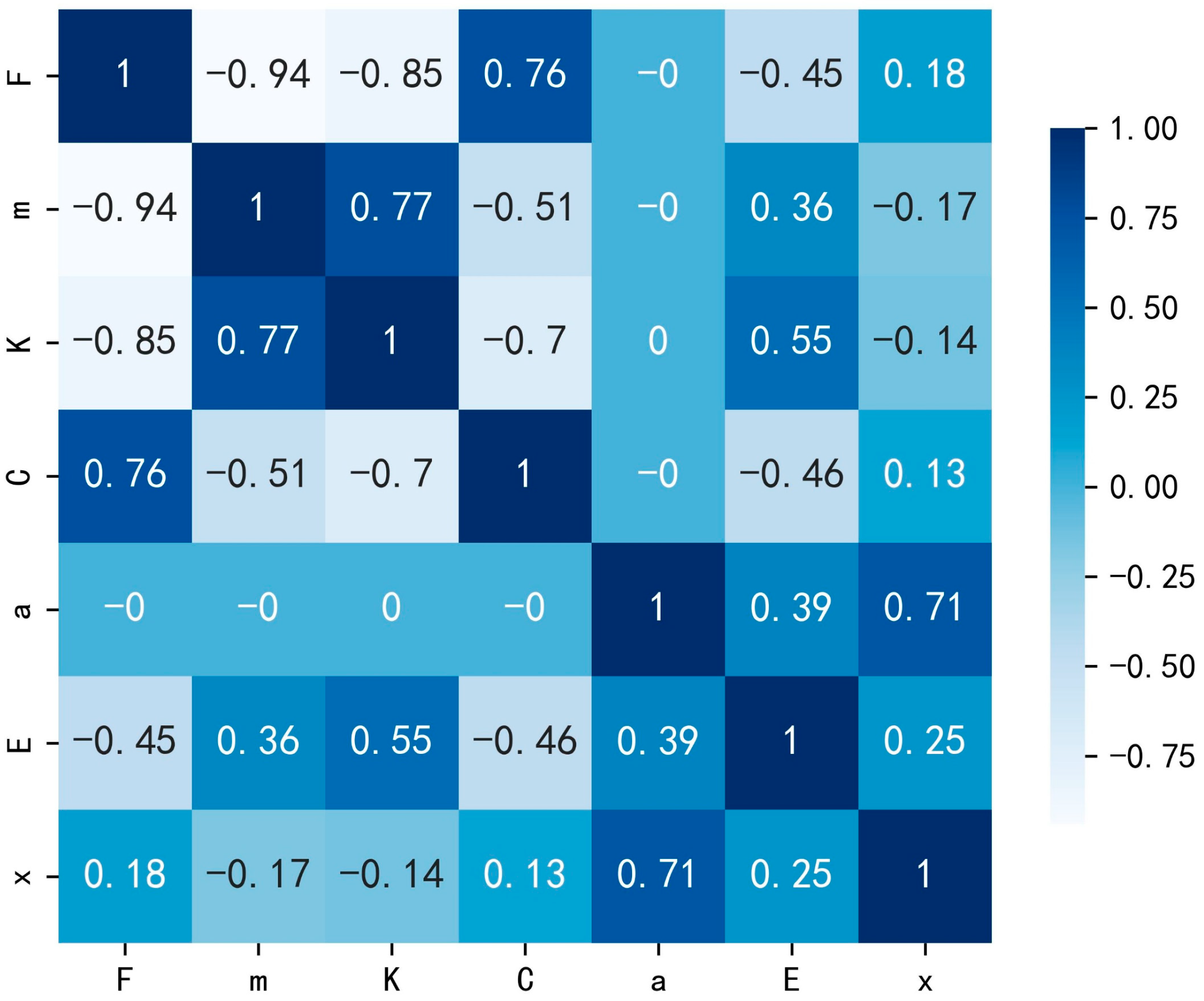
The dataset was optimized by utilizing the PCC to assess correlations among the input variables. This statistical measure evaluates the degree of linear correlation between two variables, with values ranging from −1 to 1. A high correlation coefficient between two input variables suggests a substantial linear relationship. In such cases, removing one of the input variables can optimize the dataset. Typically, a correlation coefficient absolute value exceeding 0.7 indicates a significant linear correlation.
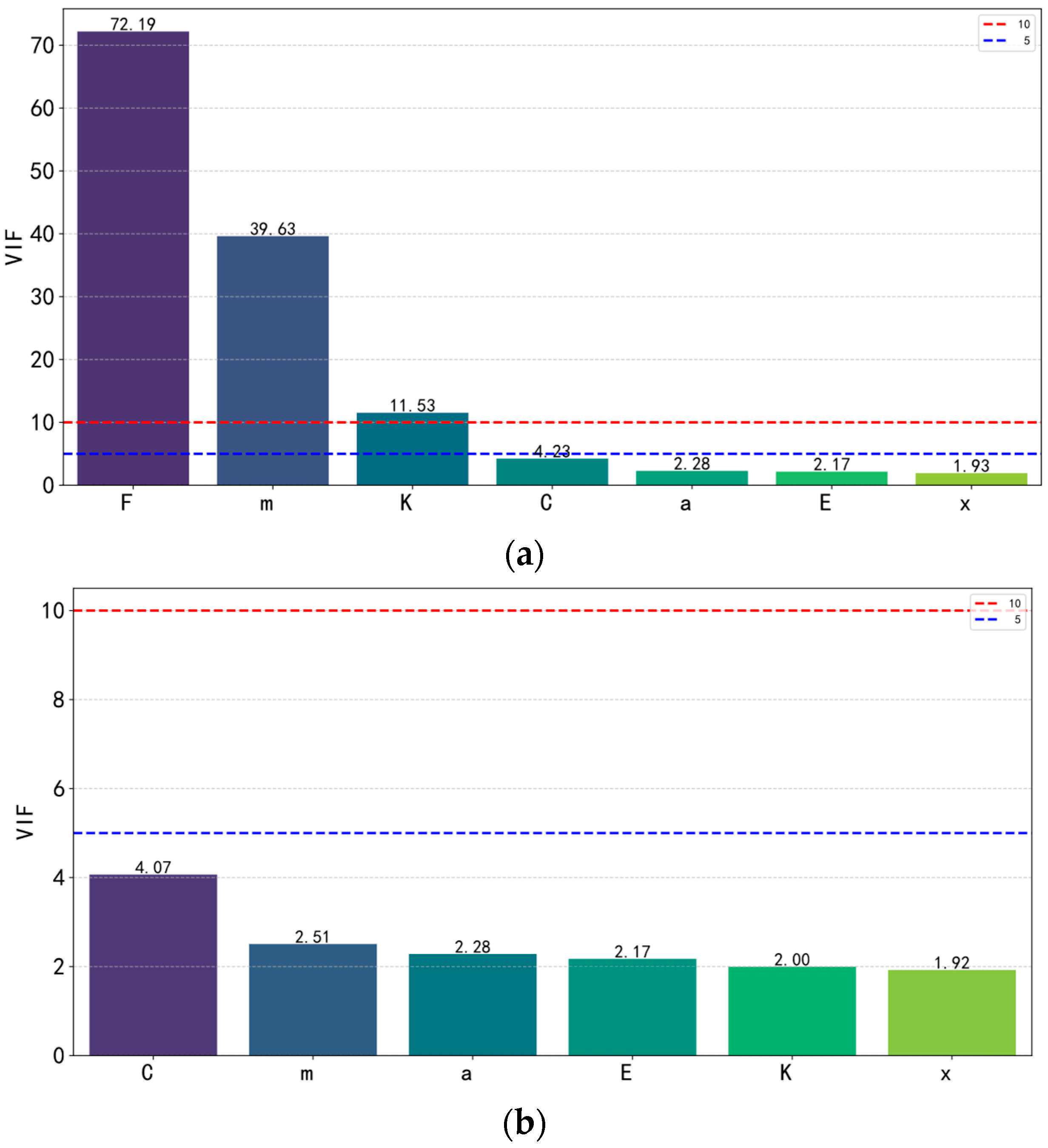
The Pearson correlation coefficients for the seven initially chosen input variables were computed and are presented in Figure 3. The Pearson correlation coefficient between the floor number and the story mass is −0.94, demonstrating a significant negative linear correlation between the two variables. As the floor number increases, the story mass decreases, showing a strong linear relationship. There are redundant variables in the dataset, and one of the input variables, either the floor number or the story mass, can be removed. The absolute values of correlation coefficients between floor number and other three building information characteristics are greater than 0.7. This situation is more complex, so the variance inflation factor (VIF) is used to quantify collinearity. Usually, it is stipulated that collinearity is serious when VIF > 10, and collinearity is high when VIF > 5. VIF analysis results are shown in Figure 4. Initial VIF analysis: From the distribution of characteristic VIF values, the VIF of floor number is 72.19, the VIF of story mass is 39.63, and the VIF of story load-bearing capacity is 11.53. The VIF of all three is higher than 10, and the collinearity is extremely strong. Among them, the VIF value of layer number is the highest, and its collinearity has the most significant effect on the model, so the layer number is deleted first. Analysis after optimization: the VIF is recalculated after deleting the layer number. At this time, the characteristic VIF values of all input variables are lower than 5, the collinearity is effectively controlled, and the independence of the feature set is significantly improved. The correlation coefficients between the floor number and the other three building information features, namely story mass, story stiffness, and story bearing capacity, all exceed 0.7. Therefore, the floor number input variable is removed from the analysis. The correlation coefficient between story stiffness and story mass is 0.77. Stiffness impacts the damage state by influencing stress distribution, energy transfer, and deformation mode. Story mass directly determines the seismic force magnitude in accordance with Newton’s second law of motion. Both parameters are indispensable and cannot be eliminated. The correlation coefficient between maximum story displacement and peak acceleration is 0.71. Maximum displacement is a structural response variable, with numerous codes regulating building structure displacements. In contrast, peak acceleration is an earthquake input variable, indicating ground motion intensity. Because they are differing features, both variables are crucial for prediction and cannot be omitted.
Engineering Implications: This optimization process yields a critical practical insight: the floor number (F), while intuitively useful, is statistically redundant for predicting story-level damage when other fundamental physical properties (mass, stiffness, capacity) are known. This is advantageous for practical applications, as it simplifies data requirements. In post-earthquake rapid assessment, obtaining precise story numbering for a damaged high-rise building can be challenging. Our model demonstrates that accurate damage prediction can be achieved using a more readily available set of six core parameters, listed in Table 7, which describe the building’s physical properties, the seismic intensity it experienced, and its resulting response.
The final selected input variables are: story mass (m), story stiffness (K), story load-bearing capacity (C), peak acceleration (a), story energy consumption (E), and maximum story displacement (x). These six parameters provide a non-redundant, physically meaningful, and efficient feature set for machine learning model training.

3. Machine Learning Algorithms

This study employs machine learning to address classification challenges in assessing the damage state of steel bundled-tube stories. The damage state is categorized into five distinct classes, forming the basis of the classification problem. Moreover, the data-driven approach of machine learning minimizes reliance on theoretical frameworks. Insights from SHAP analysis can further inform practical engineering applications and offer a theoretical foundation. Machine learning models excel in adapting to various inputs and identifying nonlinear relationships that traditional methods struggle to capture. Furthermore, they operate significantly faster than conventional assessment techniques. Consequently, machine learning-based damage assessment methods offer distinct advantages and are well-suited for assessing the damage state of steel bundled-tube stories.

3.1. Principles of Machine Learning

This study employs eight algorithms (DT, RF, KNN, SVM, NB, XGBoost, Adaboost, and CatBoost) to assess seismic damage states of steel bundled-tube stories. Table 8 details these algorithms. NB, DT, SVM, and KNN are single learning algorithms, whereas RF, XGBoost, Adaboost, and CatBoost are ensemble learning algorithms. A single learning algorithm constructs a model using its own learning capabilities to fit and predict outcomes. In contrast, ensemble learning algorithms employ multiple learning algorithms and integrate them through a specific strategy to enhance predictive performance.
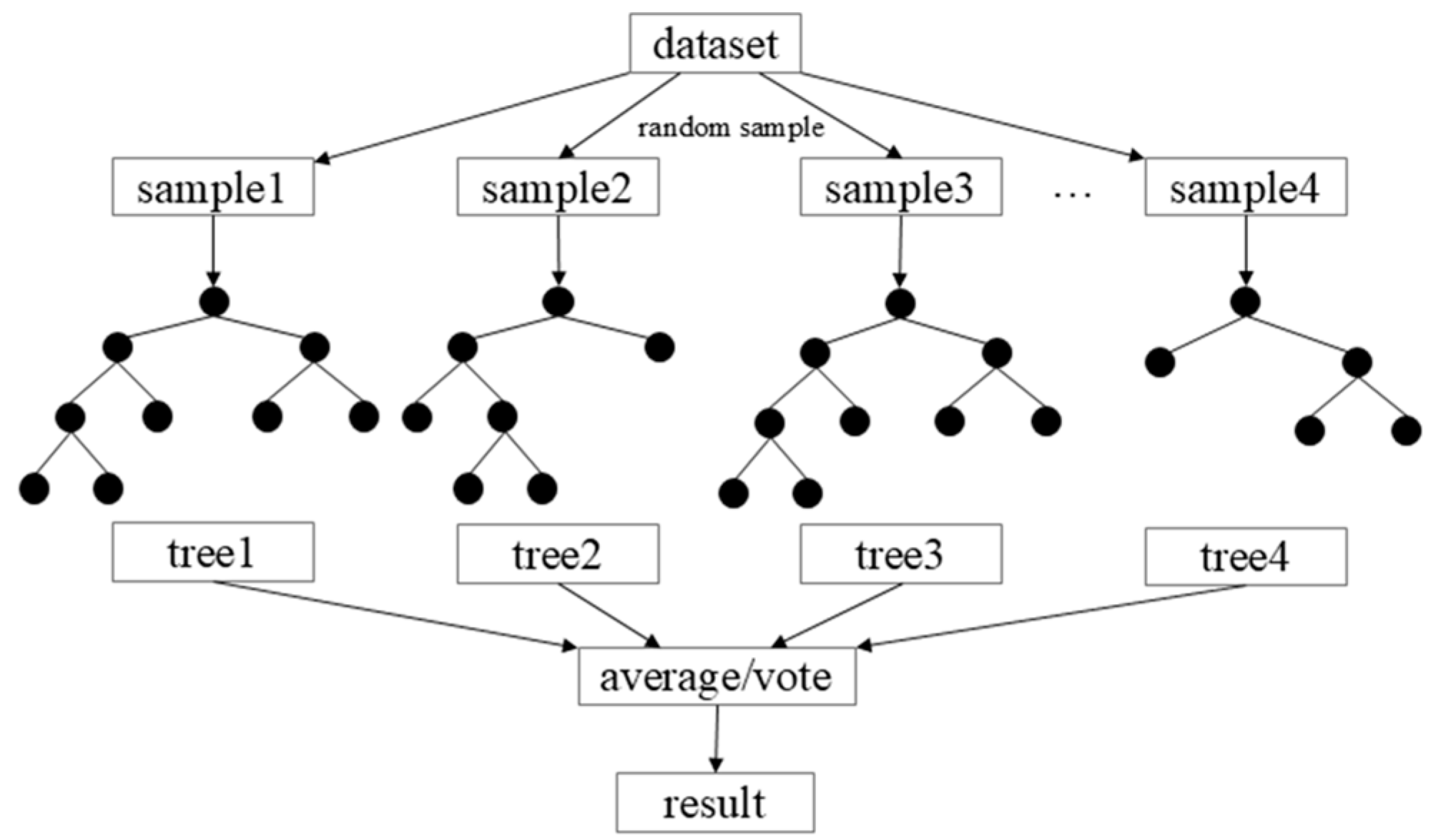
DT begins at the root node and iteratively splits data into subsets based on features, akin to a decision-making process, until each subset is homogeneous or meets a predefined stopping criterion, culminating in a leaf node. RF build on DTs by sampling multiple sub-datasets from the original data to train individual trees, selecting only a subset of features, and combining the outputs through voting or averaging to enhance model stability, as illustrated in Figure 5. The KNN algorithm identifies the nearest K samples in the training data for new data points and classifies them based on majority class judgment, while averaging target values in regression tasks. In multi-classification tasks using SVM with multi-parameter inputs (high-dimensional features), the core principle involves mapping samples in the high-dimensional feature space to a separable space and distinguishing between classes by constructing multiple classification hyperplanes. Utilizing Bayes’ theorem and assuming conditional independence among features, NB algorithm first determines the prior probability of each category. It then computes the conditional probability of features within these categories. By integrating these probabilities, NB calculates the posterior probability for the new data point’s category membership, ultimately selecting the category with the highest probability as the result. Adaboost iteratively trains multiple weak classifiers, initially assigning equal weights to all samples. During training, it directs the focus of weak classifiers towards samples with higher weights, adjusting these weights based on the error rate at the end. The classifiers are then combined to form a strong classifier. XGBoost, grounded in the additive model and gradient boosting framework, optimizes by incrementally adding weak learners, typically CART regression trees. Its primary goal is to build new trees that correct the residuals of preceding models, ultimately combining the predictions from all trees, as illustrated in Figure 6. CatBoost excels in processing categorical features without complex coding. It employs ordered target statistics to utilize category order information directly in modeling and uses symmetric tree structures to minimize prediction bias and enhance accuracy.

3.2. Machine Learning Model Training

Eight machine learning algorithms were implemented using Scikit-learn in Python 3.12 to assess damage states of steel bundled-tube stories. Figure 7 illustrates the model development process. The dataset was split into a training set (80%) for model training and a test set (20%) for performance evaluation. The dataset utilized in the study comprised 2700 data points, which were randomly partitioned into training and test sets through the “holdout” method implemented by computer [33]. This approach is efficient and convenient, facilitating the expeditious evaluation of models and the swift generation of clear performance metrics. This approach is effective for preliminary model screening and demands minimal resources. The dataset is split into a training set and a test set. The training set is used to train the machine learning model, with performance enhancements achieved through parameter optimization. The test set then evaluates the model, yielding its performance metrics. This study compares eight predictive models to assess their respective advantages and disadvantages. It experimentally validates that XGBoost and Random Forest methods, optimized via Bayesian techniques, outperform others across multiple assessment metrics, as will be elaborated in detail.

4. Machine Learning Performance Comparison

4.1. Machine Learning Evaluation Metrics

To compare the performance of various machine learning models, confusion matrices were employed for visualization. The horizontal axis represents the actual damage state, while the vertical axis indicates the predicted damage state. Diagonal values represent correctly predicted data points, while off-diagonal values indicate incorrect predictions. Model performance is assessed using accuracy, precision, recall, and F1-score. Accuracy measures the ratio of correct predictions to the total number of samples. Precision is defined as the ratio of true positive predictions to the total predicted positives. Recall measures the ratio of true positive predictions to all actual positives. The F1-score represents the harmonic mean of precision and recall. The formulas for these metrics are as follows (2)–(5).
a c c u r a c y = T P + T N T P + F P + T N + F N
p r e c i s i o n = T P T P + F P
r e c a l l = T P T P + F N
F 1 _ s c o r e = 2 × p r e c i s i o n × r e c a l l p r e c i s i o n + r e c a l l
T P (True Positive) denotes samples correctly identified as positive by the model. T N (True Negative) indicates samples accurately classified as negative. F P (False Positive) represents samples incorrectly predicted as positive, while F N (False Negative) refers to samples wrongly identified as negative.

4.2. Analysis of Prediction Results

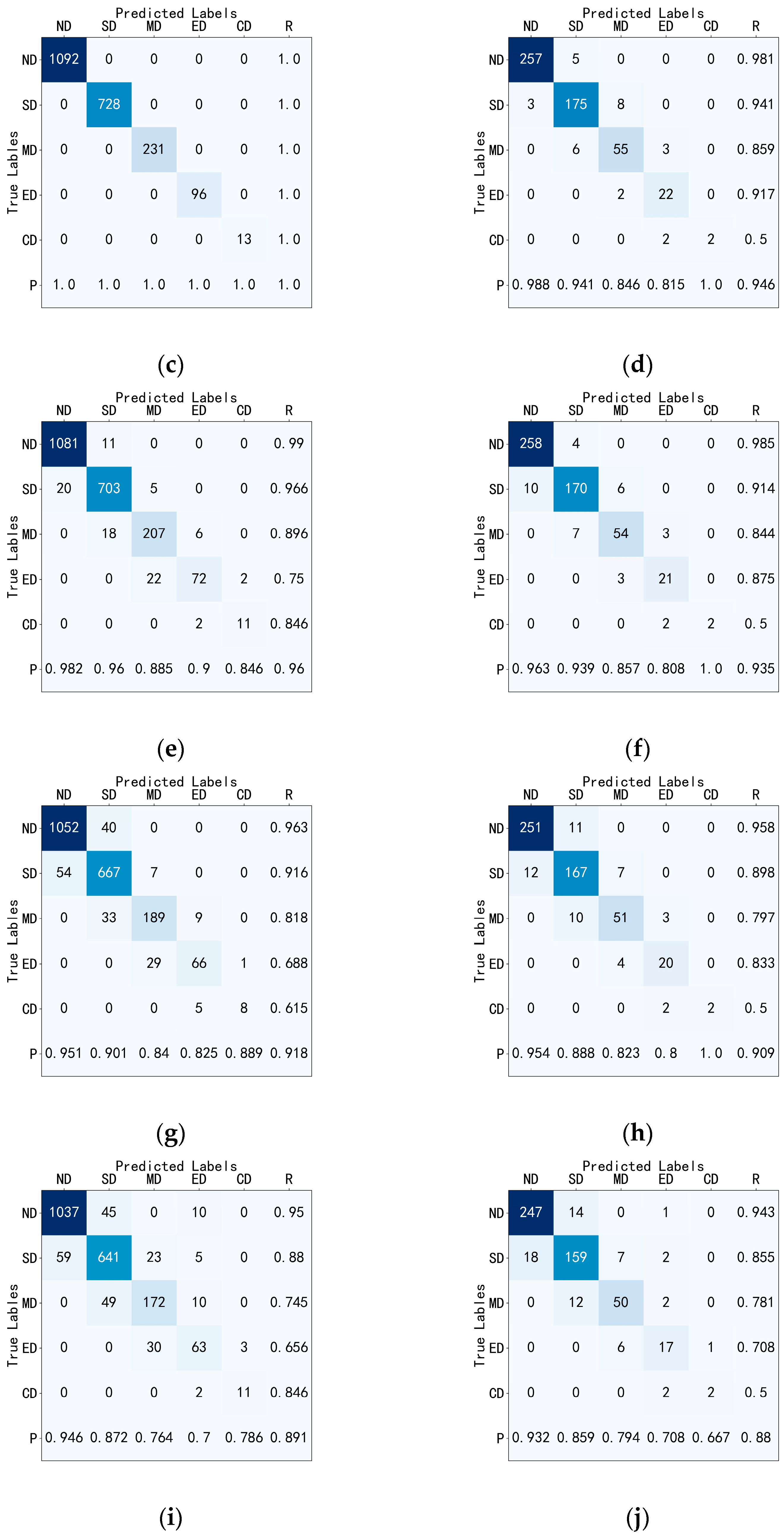
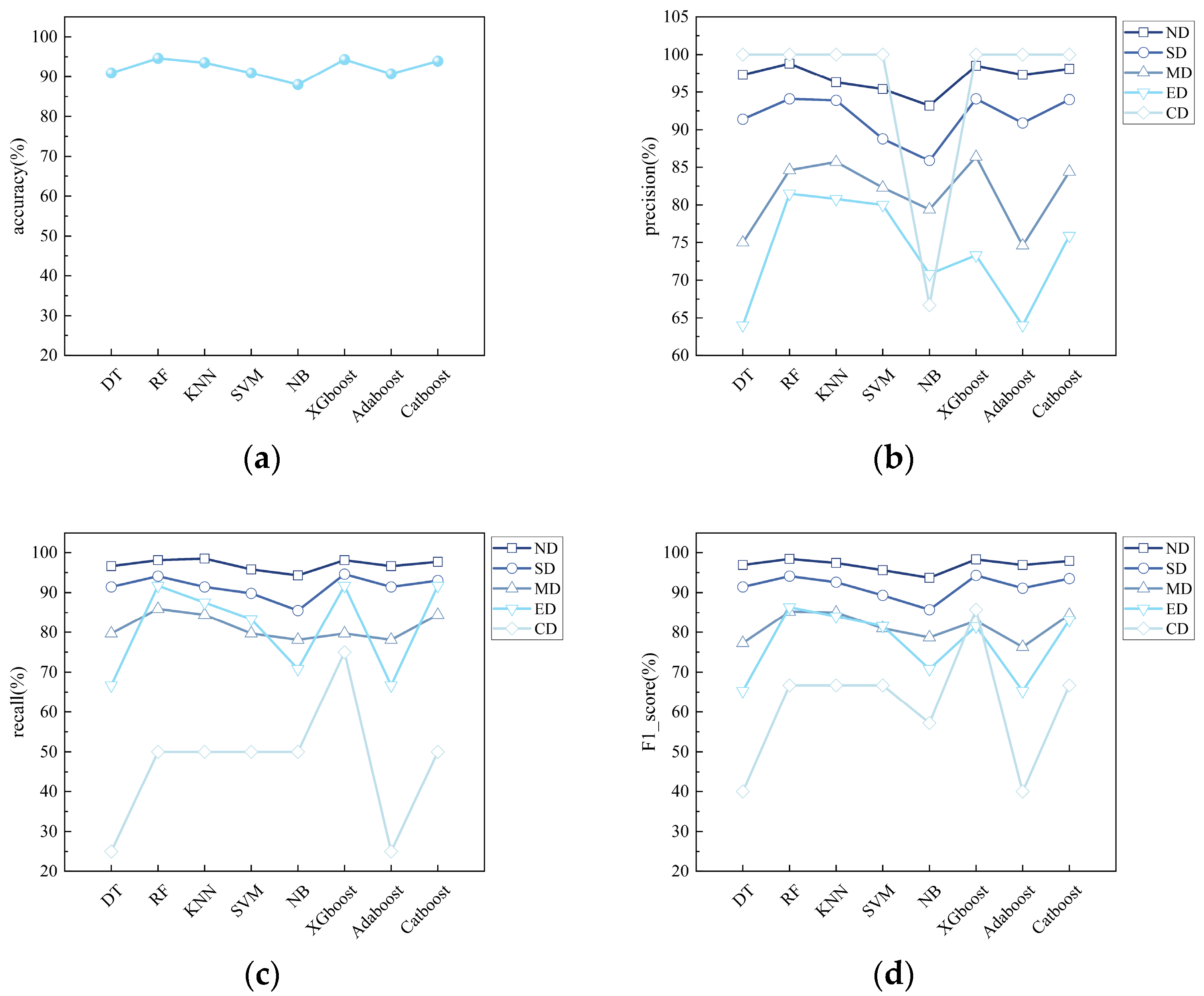
The performance of the eight machine learning models was rigorously evaluated on both training and test sets. Figure 8 presents the confusion matrices for the training and test sets across eight machine learning models. Figure 9 illustrates their accuracy, precision, recall, and F1 score. From the test set accuracy: (1) RF is the top-performing model at 94.6%, followed closely by XGBoost at 94.3%. (2) NB is the poorest performer, with training and test set accuracies of 89.1% and 88.0%, respectively, due to its assumption of feature independence and difficulty in capturing complex data relationships. (3) Models like DT achieve 100% accuracy in the training set but show reduced performance in the test set, with DT’s accuracy dropping to 90.9%, indicating overfitting.
Figure 9 illustrates that trends were consistent across all damage states except for ED and CD. Most models exhibited high precision, recall, and F1 scores when predicting ND, SD, and MD injury states. In contrast, predictions for ED and CD states showed lower scores and greater variability across models. The reason may be caused by sample imbalance. The dataset exhibits class imbalance, with ED and CD states underrepresented compared to ND, SD, and MD states. This is attributed to the steel bundled-tube structure’s robust seismic performance, which rarely reaches the ED and CD damage states during tests. Future studies should prioritize addressing the class imbalance, such as by applying techniques like the Synthetic Minority Over-sampling Technique (SMOTE) to generate more samples for the under-represented ED and CD states. For predicting the five damage states, the RF and XGBoost models excel in precision, recall, and F1 score.
This study recommends using the RF and XGBoost models for rapid assessment of seismic damage in steel bundled-tube stories. The effectiveness of machine learning models varies based on dataset characteristics. Thus, when choosing models for practical applications, it is crucial to first compare their foundational principles and then select the model that offers the highest accuracy for the specific problem.

5. Hyperparameter Optimization

Hyperparameters are the parameters set prior to model training, which directly govern the model’s architecture, training process, and generalization capacity. Existing methods for hyperparameter optimization encompass manual tuning, random search, grid search, and Bayesian optimization. Manual tuning demands significant expertise. While random and grid searches exhaustively explore the hyperparameter space to find near-optimal solutions, they fail to leverage insights from prior searches to inform future ones, leading to inefficiency. Bayesian hyperparameter optimization establishes a proxy model between hyperparameters and model performance, guiding the hyperparameter search towards more optimal values. This study employs Bayesian optimization to optimize the hyperparameters of RF and XGBoost models, leveraging the hyperopt library for the optimization process.

5.1. Fundamentals of Bayesian Optimization

Bayesian optimization is a powerful approach for optimizing objective functions, especially when evaluation costs are high. It begins by defining a search space for multiple hyperparameters. Using historical data of hyperparameter combinations and their objective function values, Bayesian optimization constructs a proxy model. This model often utilizes the Tree-structured Parzen Estimator to approximate the relationship between hyperparameters and the objective function, as described in Equation (6).
P f x x = P x f η P x f < η
where η is an interquartile threshold to distinguish well-performing regions from poorly performing regions and f x is the objective function. Next, the acquisition function is used to find a balance between exploring new hyperparameter regions and utilizing known well-performing regions to select the next set of hyperparameters to evaluate. The commonly used expectation lifting of the acquisition function is shown in Equation (7) and its closed solution is shown in Equation (8). Where μ x and σ x are the mean and standard deviation of the Gaussian process prediction at point x , f b e s t is the best-observed value of the objective function so far, and z is defined as shown in Equation (9). Here, Φ z and ϕ z represent the cumulative distribution function and probability density function of the standard normal distribution, respectively.
E I x = E max f x f b e s t , 0
E I x = μ x f b e s t Φ z + σ x ϕ z
z = μ x f b e s t σ x
The proxy model is revised for every new set of hyperparameters assessed until reaching the predetermined maximum number of evaluations. Ultimately, the hyperparameter configuration that maximizes the objective function (minimizing the negative accuracy, which corresponds to maximizing accuracy) is identified to improve the model’s performance.

5.2. Model Optimization Process

The parameter range is predetermined based on prior domain knowledge. Table 9 illustrates the roles of different hyperparameters in shaping the characteristics of machine learning algorithms. The hyperparameter search space is initially defined through cross-validation in conjunction with data features. Random Forest mitigates overfitting by using bootstrap sampling to create multiple sample subsets, combined with random feature subset selection to generate numerous weak decision trees. This leverages the variance reduction effect of the bagging ensemble strategy to suppress overfitting. Meanwhile, XGBoost controls model complexity by incorporating L1/L2 regularization terms to constrain leaf node weights, along with tree depth limitations, column sampling (feature sub-sampling), and pruning mechanisms. Additionally, it further alleviates overfitting through sub-sampling (instance sampling) and learning rate adjustment. These optimization measures work synergistically to not only enhance the model’s fitting capability to the training data but, more importantly, significantly improve its generalization performance on unseen data. Compared to other benchmark models, the meticulously tuned ensemble models demonstrate superior stability and robustness while maintaining computational efficiency. This systematic hyperparameter optimization approach provides a valuable reference for machine learning applications in the field of structural engineering, particularly in scenarios with limited data but extremely high reliability requirements.
Bayesian optimization was performed on the RF model. The optimized values are presented in Table 10. After optimization, the accuracy was 95.2%, showing an increase of 0.6%.
The XGBoost model was optimized using Bayesian optimization. The optimized values are presented in Table 11. After optimization, the accuracy reached 96.5%, showing an improvement of 2.2%.
After Bayesian optimization based on hyperparameters, the accuracy of both machine models was improved. However, the improvement of the XGBoost model is higher than that of the RF model, with an increase of 2.2%, and it has surpassed the RF model. The XGBoost model has numerous parameters, while the parameter adjustment of the RF model is relatively limited, which may result in poor optimization performance of the RF model. In conclusion, it is recommended to use the XGBoost model optimized by Bayesian optimization as the final prediction model.

6. Feature Importance Analysis

6.1. Analysis of Feature Importance Using SHAP

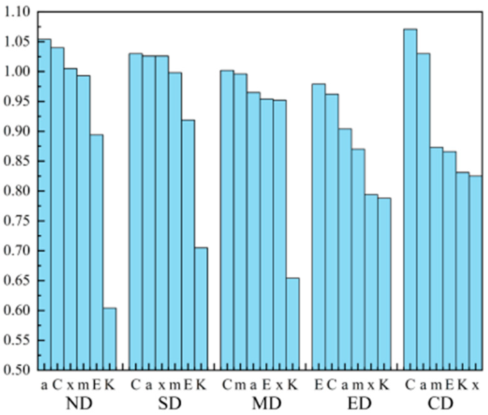
To further investigate the effect of input variables on damage state assessment, the feature importance coefficients for each input variable were extracted using the SHAP algorithm based on the best performing XGBoost model. As shown in Figure 10, from the perspective of the prediction and analysis of the seismic damage state of the steel bundled-tube stories by the SHAP plot:
(1)
Peak acceleration and story load-bearing capacity have larger coefficients of characteristic importance in all damage states, indicating that their contributions to the damage state assessment are always larger, and they are the core variables affecting the damage state assessment. The reason is twofold: peak acceleration directly reflects seismic intensity and destructive force, while story load-bearing capacity is a critical index for ensuring structural safety.
(2)
The relatively low coefficient of importance of the story stiffness feature for all damage states indicates that its contribution to the damage state assessment is small, which is attributed to the fact that there is not much difference in the stiffness of the stories, and the overall distribution of the stiffness is more homogeneous.
(3)
In assessing the ND and SD states, the maximum story displacement is more important than the story energy consumption. However, in assessing the MD, ED, and CD damage states, the story energy consumption is more important than the maximum story displacement. It is shown that displacement has a more significant effect when assessing low damage states, but not as significant as energy consumption when assessing high damage states. This is because the destruction of a structure is due to the accumulation of energy in excess of its capacity to carry and dissipate energy. Displacement is merely an indirect means and cannot fully and accurately reflect the real causes and processes of structural failure, which provides a theoretical basis for energy-based seismic design.

6.2. Engineering Implications and Design Takeaways

The SHAP algorithm can effectively reveal the relative importance of different variables under different damage states, providing theoretical support for the application of damage state assessment models and practical engineering. When evaluating the damage state, the SHAP analysis interprets the evaluation model, providing new ideas for subsequent evaluations. Attention should be paid to the quantities with significant impacts, such as input variables like story load-bearing capacity and peak acceleration. When the computational complexity is excessively high and the overall structural distribution is relatively uniform, the input variable of story stiffness may not be considered. In practical engineering, SHAP analysis is of guiding significance for building structures. During the design phase, it is necessary to reasonably design the story load-bearing capacity to ensure structural safety and meet the functional requirements. In the structural verification phase, considering both displacement and energy dissipation simultaneously can shift the structural design from the minimum code requirements to the performance—based building design. In the construction phase, devices for monitoring displacement and energy dissipation can be installed, such as displacement sensors and force sensors, to provide convenient conditions for subsequent evaluation. In the maintenance phase, this evaluation method can be used to quickly locate the weak stories, and special reinforcement schemes can be formulated for them based on the conclusions obtained from SHAP analysis. The dominance of energy dissipation in high-damage states, as revealed by SHAP analysis, suggests key practical applications. Future seismic design codes should incorporate energy-based performance indicators, particularly for critical buildings in high-seismic zones, to ensure adequate energy dissipation capacity. Additionally, force and displacement sensors could be installed in potential weak stories to monitor energy dissipation, enabling rapid post-earthquake damage assessment. For existing buildings, the model can identify vulnerable stories to guide retrofitting strategies focused on enhancing energy dissipation—such as adding dampers or improving ductility—thereby optimizing resource allocation and strengthening overall seismic performance.

7. Conclusions

This paper proposes to apply machine learning to the seismic damage state assessment of steel bundled-tube stories, which can improve the assessment speed and accuracy. To this end, multiple elastoplastic time-history analyses of the steel bundled-tube structure were conducted using ABAQUS, and 2700 data points were obtained. Eight machine learning models were selected and applied to the seismic damage assessment of the steel bundled-tube stories. The performance of different machine learning models in this practical problem was compared. Bayesian optimization was carried out on the two better models, and SHAP was used to study the influence of input variables on five damage states. The following conclusions were obtained:
(1)
When the machine learning models use the original parameters, the accuracies of RF and XGBoost rank among the top two, reaching 94.6% and 94.3%, respectively. Moreover, when evaluating the five damage states, their precision, recall, and F1_score are also ranked relatively high. After optimization, the XGBoost model improved by 2.2% and outperformed the optimized RF model, achieving an accuracy of 96.5%. Therefore, it is recommended to use the XGBoost model optimized by Bayesian optimization as the final prediction model.
(2)
Since the steel bundled-tube structure is an efficient lateral force-resistant structure, there is limited data available for high-damage states. In subsequent studies, data on high-damage states can be specifically supplemented, or the synthetic minority over-sampling technique (SMOTE) can be used to expand the dataset to improve the accuracy of the evaluation model in assessing high-damage states.
(3)
When evaluating the damage state of stories, attention should be focused on the core variables (peak acceleration and story load-bearing capacity). If the calculation volume is too large and the structural stiffness is uniformly distributed, the story stiffness may not be considered.
(4)
Displacement significantly impacts low-damage states (ND, SD), whereas energy consumption becomes dominant in high-damage states (MD, ED, CD). This indicates that there are drawbacks in the traditional seismic design that only focuses on displacement limitations. This conclusion provides theoretical basis and reference value for the energy-based seismic design, and extensive in-depth research on the energy-based seismic design should be carried out.
(5)
In engineering applications, this assessment method can be used to quickly locate the weak stories. Then, based on the SHAP analysis results, special reinforcement schemes can be formulated for the weak stories. Ultimately, the systematic optimization of the seismic performance of the steel bundled-tube structure can be achieved.

Author Contributions

Conceptualization, X.Q. and Y.H.; Methodology, Y.H.; Software, J.L.; Investigation, R.H.; Writing—original draft, J.Z.; Writing—review & editing, J.Z.; Visualization, J.L. and P.L.; Funding acquisition, X.Q. All authors have read and agreed to the published version of the manuscript.

Funding

This research was supported by the Scientific Research Project of Hebei Provincial Higher Education Institutions (QN2025322), under the Department of Education of Hebei Province.

Data Availability Statement

The original contributions presented in this study are included in the article. Further inquiries can be directed to the corresponding author.

Conflicts of Interest

The authors declare no conflict of interest.

Abbreviations

The following abbreviations are used in this manuscript:
SHAPShapley Additive Explanations
RFRandom Forest
XGBoostExtreme Gradient Boosting
PCCPearson Correlation Coefficient
CNNConvolutional Neural Network
ANNArtificial Neural Network
SVRSupport Vector Regression
DTDecision Tree
KNNK-Nearest Neighbors
SVMSupport Vector Machine
NBNaive Bayes
AdaboostAdaptive Boosting
CatBoostCategorical Boosting
NDNo Damage
SDSlight Damage
MDModerate Damage
EDExtensive Damage
CDComplete Collapse
FFloor Number
mStory Mass
KStory Stiffness
CStory Load-Bearing Capacity
aPeak Acceleration
EStory Energy Consumption
xMaximum Story Displacement
VIFVariance Inflation Factor
SMOTESynthetic Minority Over-sampling Technique

References

  1. Cheng, S.T.; Han, J.P.; Shang, J.Y. Optimal repair decision and seismic resilience analysis of seismic-damaged RC structures considering rebar corrosion. J. Build. Eng. 2025, 112, 113749. [Google Scholar] [CrossRef]
  2. Hu, B.B.; Li, S.; Hou, Z.X.; Zhai, C.H. A practical method for functional recovery analysis based on seismic resilience assessment of city building portfolios. J. Build. Eng. 2024, 95, 110304. [Google Scholar] [CrossRef]
  3. Ali, S.R.; Morteza, R.D.; Mahdi, E.; Delbaz, S. Seismic resilience evaluation of confined masonry school buildings retrofitted by shotcrete method. Soil Dyn. Earthq. Eng. 2024, 187, 108980. [Google Scholar] [CrossRef]
  4. Lu, J.F.; Li, Z.H.; Teng, J. Seismic resilience assessment for reinforced concrete frame structural systems based on complex network considering repair paths. Structures 2025, 77, 109072. [Google Scholar] [CrossRef]
  5. Tsuchimoto, K.; Narazaki, Y.; Spencer, B.F. Development and Validation of a Post-Earthquake Safety Assessment System for High-Rise Buildings Using Acceleration Measurements. Mathematics 2021, 9, 1758. [Google Scholar] [CrossRef]
  6. Ogunjinmi, P.D.; Park, S.S.; Kim, B.; Lee, D. Rapid Post-Earthquake Structural Damage Assessment Using Convolutional Neural Networks and Transfer Learning. Sensors 2022, 22, 3471. [Google Scholar] [CrossRef]
  7. Feng, D.C.; Yi, X.; Deger, Z.T.; Liu, H.; Chen, S.; Wu, G. Rapid Post-Earthquake Damage Assessment of Building Portfolios Through Deep Learning-Based Component-Level Image Recognition. J. Build. Eng. 2024, 98, 111380. [Google Scholar] [CrossRef]
  8. Wang, D.; Zhang, Y.; Zhang, R.; Nie, G.; Wang, W. Detection and Assessment of Post-Earthquake Functional Building Ceiling Damage Based on Improved YOLOv8. J. Build. Eng. 2024, 98, 111315. (In Chinese) [Google Scholar] [CrossRef]
  9. Yu, Q.M.; Yuan, X.; Xu, L.Y. Cross-Material Damage Detection and Analysis for Architectural Heritage Images. Buildings 2025, 15, 3100. [Google Scholar] [CrossRef]
  10. Zhou, K.; Shi, J.L.; Fu, J.Y.; Zhang, S.X.; Liao, T.; Yang, C.Q.; Wu, J.R.; He, Y.C. An improved YOLOv10 algorithm for automated damage detection of glass curtain-walls in high-rise buildings. J. Build. Eng. 2024, 101, 111812. [Google Scholar] [CrossRef]
  11. Ling, L.M.; Ma, G.; Hwang, H.J.; Tan, X.J. Post-earthquake detection of surface spalling and cracks in masonry buildings based on computer vision. Structures 2025, 78, 109226. [Google Scholar] [CrossRef]
  12. Xu, S.D.; Chen, H.N. Deep learning and digital twin integration for structural damage detection in ancient pagodas. Sci. Rep. 2025, 15, 28408. [Google Scholar] [CrossRef]
  13. Musella, C.; Serra, M.; Menna, C.; Asprone, D. Building Information Modeling and Artificial Intelligence: Advanced Technologies for the Digitalisation of Seismic Damage in Existing Buildings. Struct. Concr. 2021, 22, 2761–2774. [Google Scholar] [CrossRef]
  14. Gharehbaghi, S.; Gandomi, M.; Plevris, V.; Gandomi, A.R. Prediction of Seismic Damage Spectra Using Computational Intelligence Methods. Comput. Struct. 2021, 253, 106584. [Google Scholar] [CrossRef]
  15. Morfidis, K.; Stefanidou, S.; Markogiannaki, O. A Rapid Seismic Damage Assessment (RASDA) Tool for RC Buildings Based on an Artificial Intelligence Algorithm. Appl. Sci. 2023, 13, 5100. [Google Scholar] [CrossRef]
  16. Zhang, W.; Wen, J.; Dong, H.; Han, Q.; Du, X. Post-Earthquake Functionality and Resilience Prediction of Bridge Networks Based on Data-Driven Machine Learning Method. Soil Dyn. Earthq. Eng. 2024, 190, 109127. [Google Scholar] [CrossRef]
  17. Oh, B.K.; Jung, W.C.; Park, H.S. Artificial Intelligence-Based Damage Localization Method for Building Structures Using Correlation of Measured Structural Responses. Eng. Appl. Artif. Intell. 2023, 121, 106019. [Google Scholar] [CrossRef]
  18. Bhatta, S.; Dang, J. Machine Learning-Based Classification for Rapid Seismic Damage Assessment of Buildings at a Regional Scale. J. Earthq. Eng. 2024, 28, 1861–1891. [Google Scholar] [CrossRef]
  19. Chen, Q.; Yu, Z.; Li, B. Image-Based Assessment of Seismic Damage in RC Exterior Beam-Column Joints. J. Build. Eng. 2024, 97, 110971. [Google Scholar] [CrossRef]
  20. Zhang, B.; Lu, G.; Yang, C.; Yang, C.; Xu, M.; Wang, K. Seismic Damage Assessment of Bonded versus Unbonded Laminated Rubber Bearings: A Deep Learning Perspective. Eng. Struct. 2024, 321, 118996. [Google Scholar] [CrossRef]
  21. Su, A.; Cheng, J.; Wang, Y.; Pan, Y. Machine Learning-Based Processes with Active Learning Strategies for the Automatic Rapid Assessment of Seismic Resistance of Steel Frames. Structures 2025, 72, 108227. [Google Scholar] [CrossRef]
  22. He, Y.; Huang, Z.; Liu, D.; Zhang, L.; Liu, Y. A Novel Structural Damage Identification Method Using a Hybrid Deep Learning Framework. Buildings 2022, 12, 2130. [Google Scholar] [CrossRef]
  23. Bhatta, S.; Dang, J. Seismic Damage Prediction of RC Buildings Using Machine Learning. Earthq. Eng. Struct. Dyn. 2023, 52, 3504–3527. [Google Scholar] [CrossRef]
  24. Nguyen, H.D.; LaFave, J.M.; Lee, Y.J.; Shin, M. Rapid Seismic Damage-State Assessment of Steel Moment Frames Using Machine Learning. Eng. Struct. 2022, 252, 113737. [Google Scholar] [CrossRef]
  25. Wang, L.J.; Huang, C.Y.; Shan, J.Z.; Yu, H.; Su, J.R. Machine Learning Prediction Method for Seismic Damage of Existing Buildings Driven by Multiple Features. J. Build. Struct. 2024, 45, 1–12. [Google Scholar]
  26. Ni, X.; Duan, K. Machine Learning-Based Models for Shear Strength Prediction of UHPFRC Beams. Mathematics 2022, 10, 2918. [Google Scholar] [CrossRef]
  27. Zhao, C.; Zhu, Y.; Zhou, Z. Machine Learning-Based Approaches for Predicting the Dynamic Response of RC Slabs under Blast Loads. Eng. Struct. 2022, 273, 115104. [Google Scholar] [CrossRef]
  28. Naderpour, H.; Mirrashid, M.; Parsa, P. Failure Mode Prediction of Reinforced Concrete Columns Using Machine Learning Methods. Eng. Struct. 2021, 248, 113263. [Google Scholar] [CrossRef]
  29. Mangalathu, S.; Jang, H.; Hwang, S.H.; Jeon, J. Data-Driven Machine-Learning-Based Seismic Failure Mode Identification of Reinforced Concrete Shear Walls. Eng. Struct. 2020, 208, 110331. [Google Scholar] [CrossRef]
  30. Amir, A.S.; Abouzar, J.; Habib, A.B.; Zhou, Y.; Ertugrul, T. A scaling-based generalizable integrated ML-mechanics model for lateral response of self-centering walls. Eng. Struct. 2025, 336, 120326. [Google Scholar]
  31. GB 50011-2010; Code for Seismic Design of Buildings. Standardization Administration of China: Beijing, China, 2010. (In Chinese)
  32. Hao, Y.; Chen, F.; Du, C.H.; Ding, Q.Y.; Lei, H.; Hu, P.C. Seismic Damage Assessment of Floors in Vertically Stepped Steel Bundled-Tube Structures. Build. Sci. 2024, 40, 154–163. (In Chinese) [Google Scholar]
  33. Raschka, S. Model Evaluation, Model Selection, and Algorithm Selection in Machine Learning. arXiv 2018, arXiv:1811.12808. [Google Scholar]
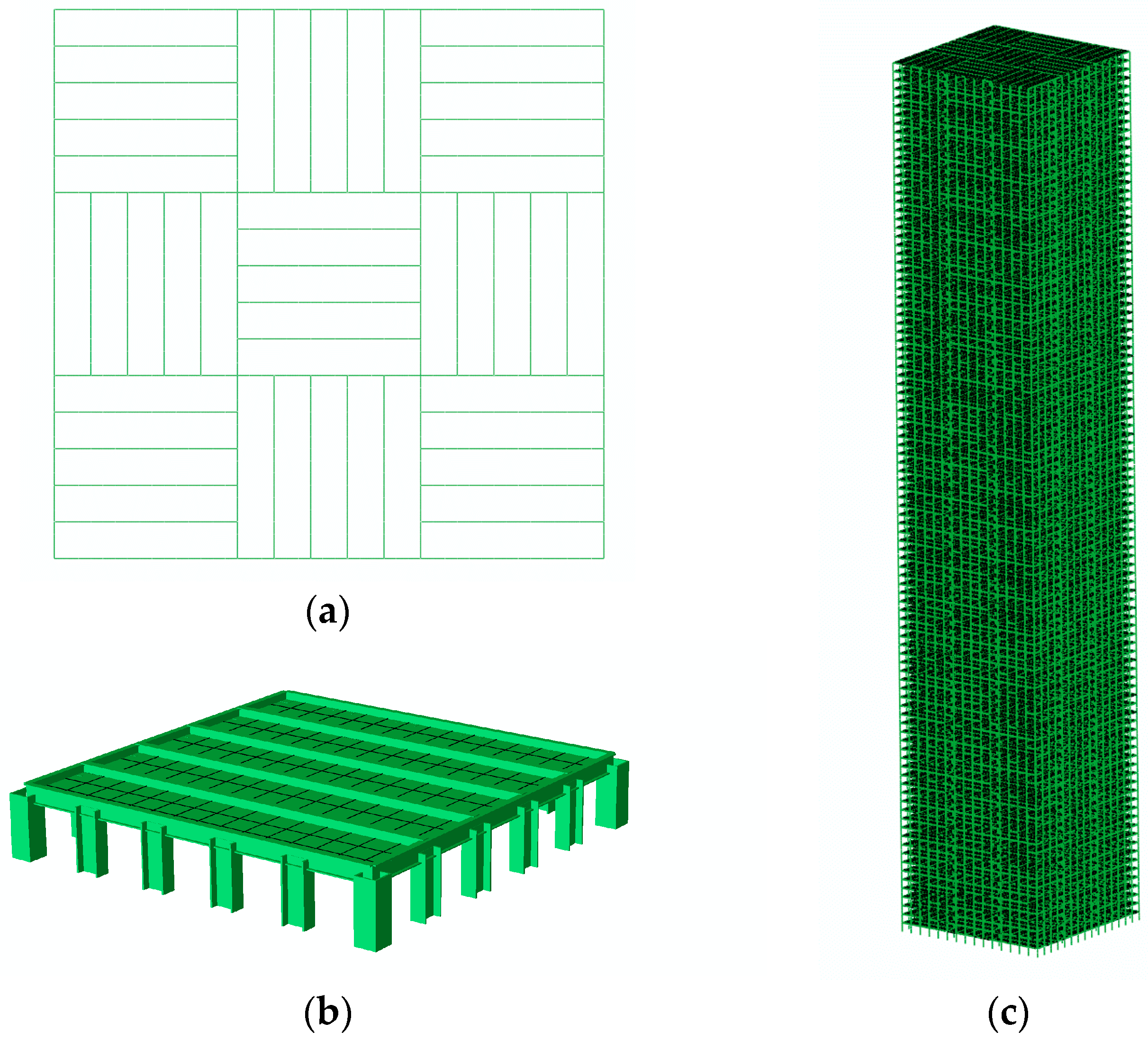
Figure 1. Elastoplastic model of steel bundled-tube: (a) Ground floor plane, (b) Framed tube unit, (c) Overall structure.
Buildings 15 03758 g001
Figure 2. Seismic damage distribution of the steel bundled-tube stories.
Buildings 15 03758 g002
Figure 3. Pearson correlation coefficient.
Buildings 15 03758 g003
Figure 4. VIF Analysis Results: (a) Before removing F, (b) After removing F.
Buildings 15 03758 g004
Figure 5. Basic flow of RF model.
Buildings 15 03758 g005
Figure 6. Basic flow of XGBoost model.
Buildings 15 03758 g006
Figure 7. Flowchart of the machine learning model.
Buildings 15 03758 g007
Figure 8. Machine learning confusion matrix: (a) DT training set, (b) DT test set, (c) RF training set, (d) RF test set, (e) KNN training set, (f) KNN test set, (g) SVM training set, (h) SVM test set, (i) NB training set, (j) NB test set, (k) XGBoost training set, (l) XGBoost test set, (m) Adaboost training set, (n) Adaboost test set, (o) CatBoost training set, (p) CatBoost test set.
Buildings 15 03758 g008aBuildings 15 03758 g008bBuildings 15 03758 g008c
Figure 9. Visualization of machine learning performance metrics: (a) accuracy, (b) precision, (c) recall, (d) F1_score.
Buildings 15 03758 g009
Figure 10. Importance coefficients of SHAP in XGBoost.
Buildings 15 03758 g010
Table 1. Cross-sectional dimensions of the steel bundled-tube components.
Name of MemberSection FormSize of Member
(mm × mm × mm × mm)
Section Form
Corner columnBox section1300 × 1300 × 100 × 1001–100
Side columnH-section1400 × 900 × 90 × 1001–30
1400 × 900 × 60 × 8031–60
1400 × 900 × 40 × 6061–100
Skirt beam1000 × 400 × 50 × 701–60
1000 × 400 × 35 × 5061–100
Main beam1100 × 500 × 30 × 501–100
Table 2. Comparison of Modal Analysis Results between PKPM and ABAQUS.
PKPMABAQUSPKPM/ABAQUS
T1/s7.387.4299.5%
T2/s7.387.4299.5%
T3/s4.914.91100%
M/105t4.934.83100%
Table 3. Identified criteria for damage states.
Component TypePercentageSlightObvious IObvious IIObvious IISevere
Steel column
(plastic strain)
0~5%0.0160.0180.020.0250.035
5%~20%0.0650.070.080.10.14
20%~40%0.1650.170.180.20.24
40%~60%0.2650.270.280.30.34
60%~80%0.3650.370.380.40.44
>80%0.4650.470.480.50.54
Steel skirt beam (plastic strain)0~5%0.0050.010.0150.020.025
5%~20%0.020.040.060.080.1
20%~40%0.040.060.080.10.12
40%~60%0.060.080.10.120.14
60%~80%0.080.10.120.140.16
>80%0.10.120.140.160.18
Floor slabs
(characterized by plastic strain in floor reinforcement)
0~5%0.0020.0040.0060.0080.01
5%~20%0.020.0250.030.0350.04
20%~40%0.0250.030.0350.040.045
40%~60%0.030.0350.040.0450.05
60%~80%0.0350.040.0450.050.055
>80%0.040.0450.050.0550.06
Table 4. Connection between the damage degree of steel members and the unit plastic strain.
Damage DegreePlastic Strain of Elements
IntactNon-plastic strain
SlightPlastic strain ≤ 0.2%
obvious0.2% < Plastic strain ≤ 6%
SeverePlastic strain > 6%
Note: The “Obvious” deformation range is further subdivided into three zones based on plastic strain magnitude: Deformation Zone I (0.2% < plastic strain ≤ 2%), Deformation Zone II (2% < plastic strain ≤ 4%), and Deformation Zone III (4% < plastic strain ≤ 6%).
Table 5. Corresponding relationship between damage factors and damage states.
Damage
States
No
Damage
Slight
Damage
Moderate
Damage
Extensive
Damage
Complete
Damage
Damage
factors
0~0.20.2~0.40.4~0.60.6~0.9≥0.9
Table 6. Value ranges of each input variable.
Input
Variables
F
(Floor)
M
(t)
K
(kN/m)
C
(kN)
A
(Gal)
E
(J)
X
(m)
minimum value14622.3974,0001,330,00022048030.000997
maximum value1005088.458,700,0002,080,00040004,202,560,00012.805
average value50.54845.312,594,5401,792,9002008138,495,7114.023
Table 7. Rationale for Final Input Variable Selection.
CategoryVariableRetained/RemovedEngineering Rationale
Building informationFRemovedHigh multicollinearity (VIF > 70). Redundant when mass, stiffness are known.
mRetainedFundamental property determining inertial forces.
KRetainedGoverns stress distribution and dynamic response.
CRetainedDirectly related to structural safety margin.
Earthquake informationaRetainedPrimary indicator of ground motion intensity.
Response
Response
ERetainedCritical indicator of cumulative damage.
xRetainedKey serviceability and safety limit state parameter.
Table 8. Machine learning algorithms.
NumberAlgorithm NameClassification of Machine Learning Algorithms
1DTSingle learning
2RFEnsemble learning
3KNNSingle learning
4SVMSingle learning
5NBSingle learning
6XGBoostEnsemble learning
7AdaboostEnsemble learning
8CatBoostEnsemble learning
Table 9. Hyperparameters of RF and XGBoost to be optimized.
HyperparametersFunction
n_estimatorsRepresents the number of decision trees in the forest.
max_depthLimit the maximum depth of each decision tree to prevent overfitting.
max_featuresAvoid training all decision trees based on the same features, thereby enhancing the generalization ability of the model.
learning_rateBalance the convergence speed and accuracy of the model
subsampleIntroduce randomness to reduce overfitting.
colsample_bytreeFurther increase the diversity among decision trees to prevent all decision trees from being trained based on the same features.
gammaThe minimum loss reduction used to control node splitting prevents the decision tree from over—splitting and avoids overfitting.
reg_alphaL1 regularization penalties are respectively imposed on the weights of the model to make the weights of the model sparser.
reg_lambdaL2 regularization penalties are respectively imposed on the weights of the model to make the weights of the model smaller.
Table 10. Optimized parameters of the RF model.
HyperparametersOptimized Values
n_estimators96
max_depth12
max_features2
bootstrapFalse
class_weightbalanced
criteriongini
Table 11. Optimized parameters of the XGBoost model.
HyperparametersOptimized Values
n_estimators119
max_depth30
learning_rate0.6274635497594659
subsample0.30713949719439915
colsample_bytree0.8246860247165366
gamma0.0403280338923106
reg_alpha0.5536200711976728
reg_lambda0.4993919951300849
Disclaimer/Publisher’s Note: The statements, opinions and data contained in all publications are solely those of the individual author(s) and contributor(s) and not of MDPI and/or the editor(s). MDPI and/or the editor(s) disclaim responsibility for any injury to people or property resulting from any ideas, methods, instructions or products referred to in the content.