Field Dynamic Testing and Adaptive Dynamic Characteristic Identification of Steel Tower Structures in High-Speed Railway Stations Under Limited Sensor Configurations

Abstract

In the context of complex operational environments and limited sensor configurations, modal identification of large-scale tower structures often faces challenges related to adaptive model order determination and modal aliasing. This study develops an algorithmic framework for automatic mode identification based on the corrected Akaike information criterion (AICC) and adaptive density-based clustering. First, unlike traditional singular entropy increment (SEI) methods where the determined model order is affected by cumulative thresholds, the AICC-based approach ensures that the adaptively determined model order remains stable. Furthermore, automatic model order selection using the AICC is integrated with adaptive density-based clustering, where the modal assurance criterion extended to a complex mode space (MACXP) is employed to define a modal distance metric. The proposed framework enhances automatic modal clustering and mode-shape discrimination under limited sensor conditions. Finally, a field application was carried out on A-shaped steel towers of integrated bridge–station structures in a high-speed railway station to identify and validate their dynamic characteristics. The results demonstrate that (i) AICC-based model order selection effectively overcomes the threshold dependence of SEI, ensuring improved stability and reliability; (ii) combining AICC-based order determination with density-based clustering enables stable and automated modal identification; and (iii) compared with the conventional MAC, MACXP exhibits superior mode shape discrimination capability under sparse measurement conditions and clearly reveals differences in the modal characteristics of complex structures. This study provides an effective approach for model order determination, mode discrimination, and automated modal identification of large-scale engineering structures under limited sensor deployments.

1. Introduction

Steel structures of railway passenger stations are prone to stiffness degradation and cumulative damage under complex operating environments and long-term service. Coupled effects of environmental loads, train-induced aerodynamics, fatigue, and corrosion further accelerate deterioration. Reliable modal identification and condition assessment based on field vibration testing are therefore essential for structural safety and durability [1,2,3]. Compared with forced-vibration approaches, operational modal analysis (OMA) [4] identifies natural frequencies, damping ratios, and mode shapes solely from ambient excitation and structural responses. Due to its economy and practicality, OMA has been widely used for the health monitoring of large civil structures—such as bridges [5], tall buildings [6], hydraulic dams [7], and heritage constructions [8]—and has developed systematic methodologies in the frequency, time, and time–frequency domains. Among these, the stochastic subspace identification (SSI) method [9] has become the most widely used owing to its numerical stability and strong noise robustness. However, state-space-based SSI relies heavily on the accurate selection of the model order during computation. When constructing stabilization diagrams by varying model orders, the method faces challenges such as modal aliasing and spurious modes, which hinder the accuracy and automation of OMA [8,10].

Accurate model order selection is essential for reliable modal identification. An order that is too high introduces spurious poles, resulting in non-physical modes. An order that is too low may merge different physical modes or noise components into a single mode, causing so-called mode splitting and concealing the true dynamic properties of the structure [4,11]. In engineering practice, empirical lower bounds often help reduce computational effort. A minimum order of two is commonly used. Ubertini et al. [5] suggested taking twice the number of peaks in the power spectral density (PSD) of the response data as the minimum order to ensure inclusion of all dominant modes. For the upper bound, many studies adopt the singular entropy method based on singular value decomposition (SVD). The core idea is that as the model order increases, the singular entropy of the system matrix converges; the order at which entropy stabilizes can be taken as the maximum model order. Variants of this approach use the first derivative [12,13] or curvature [14] of the singular-entropy increment to assist in the decision. In addition, Teng et al. [15] proposed comparing the norm difference between the original Toeplitz matrix and an estimated Toeplitz matrix truncated by singular values, and taking the minimum difference as the criterion for maximum order. Pourgholi et al. [16] examined the trend of the Toeplitz matrix condition number and concluded that convergence of this parameter indicates that the order sufficiently captures all dynamic characteristics. Zhang et al. [17] introduced an information-entropy-based criterion to balance model fit and complexity, and applied the Akaike information criterion (AIC) to select the order of autoregressive moving average (ARMA) models.

In the aspect of modal identification, the core challenge in mode shape discrimination lies in accurately distinguishing the similarity between modes of different orders. The classical modal assurance criterion (MAC) has been widely adopted due to its computational simplicity and intuitive clarity. However, under conditions such as sparse sensor placement, limited degrees of freedom in observations, or the presence of in-plane/out-of-plane modal coupling, the off-diagonal terms of MAC often become excessively large. This leads to an overestimation of similarity between different modes, resulting in the phenomenon of “modal aliasing” [18,19]. Vacher et al. [20] proposed the extended modal assurance criterion (MACXP) by generalizing modal vectors to complex space. This approach simultaneously considers both real and imaginary parts of modes, significantly enhancing modal discrimination in complex damped systems or complex modal scenarios. Compared to traditional MAC, MACXP is particularly suitable for assessing mode similarity under sparse sensor configurations. HE et al. [19] introduced the modified modal observability correlation (MMOC). By incorporating input-output observability weighting factors in its definition, this method demonstrates superior discrimination capability and robustness under spatial modal overlap.

In the field of stabilization diagram interpretation for OMA, physical modes usually appear as dense pole clusters that recur across different model orders, whereas noise and spurious modes are scattered. Conventional practice relies on manual delineation of cluster boundaries, which is time-consuming and prone to subjectivity. To reduce manual involvement and enhance consistency, recent research has shifted toward density-based clustering frameworks. Density-based spatial clustering of application with noise (DBSCAN) has emerged as a key automated OMA approach due to its ability to identify clusters of arbitrary shapes without requiring predefined cluster counts, coupled with its inherent noise detection capabilities [10,21]. Its key hyperparameters are the neighborhood radius ε (Eps) and the minimum number of points (MinPts). Ester et al. [22] reported that DBSCAN is relatively insensitive to MinPts, which is commonly set to about twice the data dimension, so the main parameter adjustment can focus on ε. Once MinPts is fixed, ε is often determined from the “elbow” of a k-nearest-neighbor (k-nn) distance plot [22]. However, the elbow lacks a rigorous definition for discrete data and may present multiple or weak elbows, which limits full automation. To overcome these limitations, Ye and Zhao [23] suggested setting MinPts based on the maximum model order of the stabilization diagram and using a small fixed ε to match the physical intuition of very small distances between points in a true modal cluster. Boroschek and Bilbao [24] also used the maximum model order to determine MinPts but adopted OPTICS to avoid a single ε and proposed an automated recognition strategy based on the reachability curve. Civera et al. [25] employed the silhouette coefficient to adaptively determine MinPts within a candidate range and then applied the elbow method to define ε. More recently, Bhusal and Tezcan [21] replaced visual elbow detection with an extremum criterion derived from a smoothed k-nn distance histogram, which further improves the reproducibility of ε selection.

In summary, some progress has been achieved in the dynamic characterization of large and complex structures. However, stable and fully automated modal identification under limited sensor conditions remains a challenge. The main difficulties lie in the limited stability of model-order determination methods, the restricted ability to distinguish mode shapes, and the inadequate automation in modal clustering. This study focuses on two key aspects: adaptive model-order determination and mode-shape discrimination. To ensure a complete automated modal identification process, a density-based clustering (DBSCAN) approach is also incorporated for the interpretation of stabilization diagram. The proposed algorithm integrates the corrected Akaike information criterion (AICC), covariance-driven stochastic subspace identification (SSI-COV), and the complex-domain modal assurance criterion (MACXP). It is applied to field vibration tests of a high-speed railway station steel tower. The method achieves systematic identification and verification of structural modal parameters under limited sensor conditions, and provides a reference for dynamic testing and service-state evaluation of similar large and complex structures.

The remainder of this paper is organized as follows. Section 2 introduces the structural background of the case study, which focuses on A-shaped steel towers in the bridge–station combined structures of high-speed railway stations. Section 3 describes the setup and implementation of the on-site ambient excitation tests. Section 4 details the dynamic characteristic identification methodology, including frequency-domain analysis based on the Average Normalized Power Spectral Density, automatic model-order determination, and improved density-based clustering of stabilization diagram poles. Section 5 presents and discusses the identified modal results, with a comparative analysis of modal parameter differences between the reinforced and unreinforced tower structures. Finally, Section 6 summarizes the findings and highlights their engineering significance.

2. Structural Overview

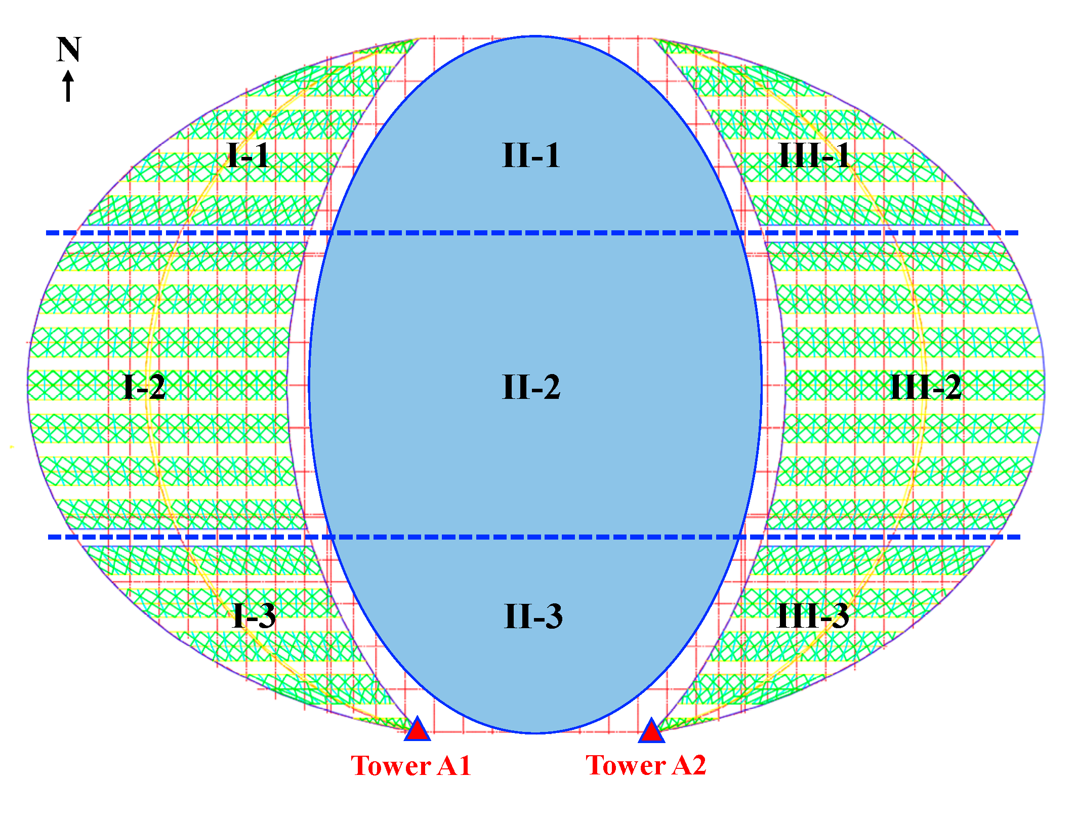
The railway passenger station adopts the design of bridge-station combined structure (Figure 1). The superstructure consists of the central station building (Zone II) and two side platform canopies (Zones I and III) (Figure 2). Each canopy forms a spatial structural system composed of A-shaped steel towers (double-limb lattice columns) and cantilevered I-beam girders. Expansion joints divide the canopy into six structural units that are symmetrically arranged with respect to the station building center. On each side of the station building, the canopy contains 15 two-span prestressed steel truss cantilever girders, with a maximum span of 66 m. The main cantilever girders are assembled from curved I-section beams. The supporting structure is made of A-shaped tower columns with heights ranging from 16.84 m to 31.5 m. The primary cross-sections of the vertical members and beams are box-shaped, while the diagonal bracings adopt circular steel tubes. All structural members are fabricated from Q345 steel. Each A-shaped column connects to its foundation through a hinged bearing. The pin in the hinged bearing has a diameter of 200 mm and is made of 40Cr steel. The gusset plates have a thickness of 80 mm and are fabricated from Q345 steel.

In terms of the load-resisting system, the vertical load-bearing mechanism consists of cantilevered I-beams, large A-shaped tower columns, and prestressed cables (Figure 3). Under downward vertical loads, the I-beams mainly provide tensile stiffness. Under upward wind loads, the cantilevered I-beams act as arches and rely on their bending stiffness to bear the loads. For lateral resistance, three groups of large A-shaped towers carry the transverse loads in the east–west direction, with every three spans of I-beams forming a braced group in the out-of-plane direction. In the north–south direction, the A-shaped towers, inclined cantilever beams, and transverse steel tubes are connected to form a portal frame that resists horizontal forces. Due to the long cantilever spans, the beam ends generate significant horizontal tension on the columns, which produces large bending moments at the column bases. The expanded cross-section at the base of each A-shaped tower column effectively increases the overall bending capacity and improves the load-bearing efficiency of the canopy structure, ensuring that performance requirements are met under various loading conditions.

The station has been in service for more than ten years. In June 2022, a special inspection was carried out on 94 hinged bearing pins of the A-shaped towers. Nine locations were found with detached cover plates, mostly concentrated in the southwest area. As shown in Figure 4a, the Tower A1 exhibited significant pin slippage, with a measured displacement of 56 mm. Before the inspection, temporary steel-pipe bracing was installed to prevent further movement. After the inspection, the A1 pin was repaired using a hydraulic jack to push it back into position (Figure 4b), and steel plates were added on the outside as limiting stops. All detached cover plates were reinstalled as well.

3. In Situ Ambient Excitation Test

To further clarify the current service condition of the A-shaped towers, structural dynamic tests were conducted on 24 December 2024, for the Towers A1 and A2, which are symmetrically located at the southwest and southeast corners of the station (Figure 2). No significant pin slippage was detected on the Tower A2, and therefore no reinforcement was applied. The two towers share identical structural configuration, member cross-sections, and materials, and are arranged with axial symmetry. These features made them suitable for ambient excitation tests to compare their dynamic characteristics.

3.1. Test Equipment and Parameter Setup

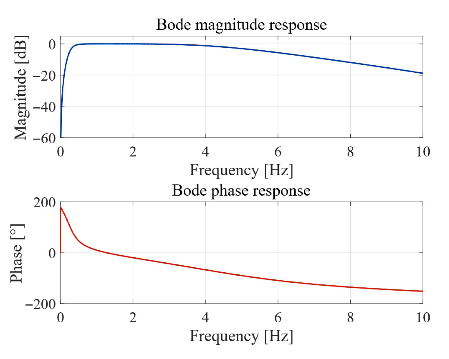
Data were recorded with a 16-channel INV3062 acquisition unit developed by the Beijing Oriental Institute of Vibration and Noise Technology (Beijing, China). The vibration pickup was type 891-2, set to the acceleration range, with a measurement capacity of 20 g and a sensitivity of 0.1 V/g. Each sensor was fixed and leveled using modeling clay and a spirit level. Testing commenced after 23:00 at night, with a sampling frequency of 128 Hz and a sampling duration of 20 min. The total data collected across all measurement points amounted to 153,600 data points. Additionally, ambient excitation test inevitably faces interference from external uncertain signals (including construction vehicle operations, nighttime bus traffic, and idling trains at the passenger station). This can introduce significant signal noise, reducing the signal-to-noise ratio of the target signal. Before analysis, the raw signals were preprocessed. The procedure included zero-mean correction to remove offsets, detrending with the least-squares method, and fourth-order Butterworth high-pass and low-pass filtering with cut-off frequencies of 0.3 Hz and 5 Hz, respectively.

3.2. Sensor Layout Plan

Tests on the Towers A1 and A2 were conducted under two operating conditions. As shown in Figure 5, six measurement points (denoted as #1–#6 in the figures) were arranged for each condition using an aerial work platform, with detailed locations listed in

Table 1. Statistics of Measurement Point Information.

No.	Position	Direction
#1	Tower top	Longitudinal horizontal (in-plane)
#2	Tower top	Lateral horizontal (out-of-plane)
#3	West side of the tower beam	Longitudinal horizontal (in-plane)
#4	West side of the tower beam	Lateral horizontal (out-of-plane)
#5	East side of the tower beam	Longitudinal horizontal (in-plane)
#6	East side of the tower beam	Lateral horizontal (out-of-plane)

. Out-of-plane measurement points on both sides of the tower beams (south–north direction) were used to identify possible out-of-plane torsion. In-plane points on both sides of the beams (east–west direction) served to verify signal consistency. Two points located along the same short beam can be regarded as belonging to a single rigid body and should exhibit identical responses, including mode-shape phase and amplitude, in all mode orders.

This study focused on identifying the first three modes of the large high-speed railway station towers, including natural frequency, mode shape, and damping ratio. The reasons are as follows:

(i)

field measurements were carried out under ambient excitation without artificial external input;

(ii)

because of the structural form, operational requirements, and sensor layout constraints, sensors could be installed only at the beam and top sections. Higher-order modes with more than two inflection points along the tower height cannot be effectively captured under the current measurement configuration.

4. Automatic Identification Method for Dynamic Characteristics

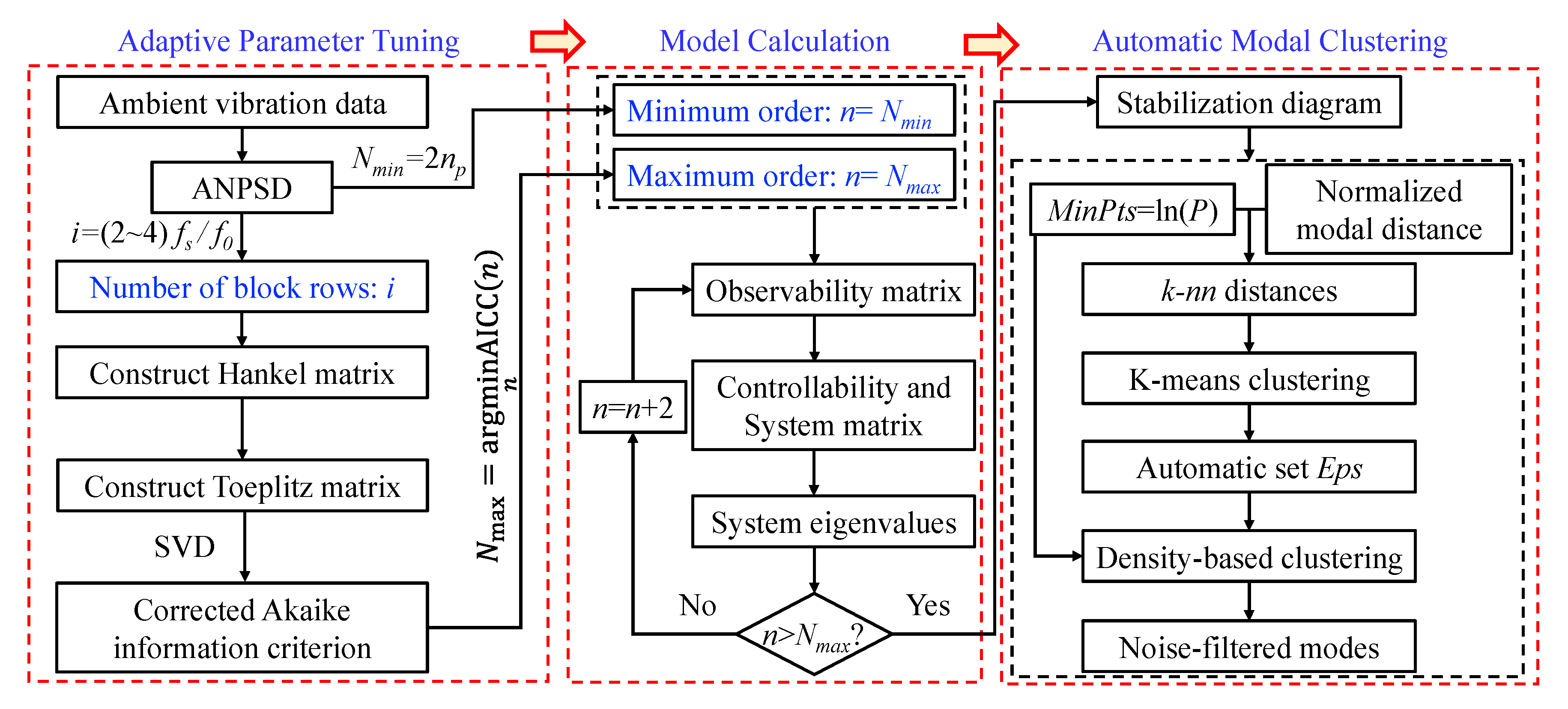
The proposed identification procedure (Figure 6) consists of three stages. (1) Parameter-adaptive tuning: the average normalized power spectral density (ANPSD) is computed from the measured responses to determine the target frequency band. A Hankel matrix with a specified block row size i is constructed, the covariance of the response is computed to form a Toeplitz matrix, and singular value decomposition (SVD) is applied to the Toeplitz matrix to extract the singular value spectrum. The lower bound of the model order is set to twice the number of distinct peaks in the ANPSD, while the upper bound is determined by minimizing the corrected Akaike information criterion (AICC), ensuring data-driven and optimally tuned parameters for subsequent analysis. (2) Model computation: system matrices are estimated sequentially for each candidate model order, and modal parameters are extracted via eigenanalysis to construct the stabilization diagram. (3) Modal clustering and discrimination: a new modal distance metric is defined using the modal assurance criterion extended to the complex modal domain (MACXP), and density-based clustering is applied to achieve automatic modal clustering and mode-shape discrimination under limited sensor conditions.

4.1. Frequency Domain Spectrum Analysis Based on ANPSD

This paper employs modal identification based on the frequency-domain Welch method and the time-domain SSI-Cov method [9]. The Pwelch method divides the random vibration signal into multiple segments, allowing overlap between segments. It calculates the power spectrum for each segment and then averages them. Due to its rapid and efficient nature, it serves as the foundational method for analysis. In this test, assuming the maximum random error ${\epsilon }_r$ in estimating the random vibration power spectrum does not exceed 10%, the required number of averaging segments $n_d$ should satisfy Equation (1) [26], i.e., 1/(0.1²) = 100. Considering that the dominant structural frequencies are below 5 Hz, the data were resampled at 32 Hz. With a 50% overlap between segments and a Hanning window, each time-history segment length NFFT was set to 760, yielding a frequency-resolution bandwidth of 0.042 Hz, i.e., f_s/NFFT = 0.042.

$$n_d={\displaystyle \frac{1}{{\epsilon }_r^2}}$$

(1)

where ${\epsilon }_r$ denotes the maximum random error in estimating the random vibration power spectrum, and $n_d$ refers to the average number of segments required by the Pwelch method.

Furthermore, structural ambient vibration tests are usually carried out at multiple measurement points. To avoid the risk that some points may coincide with vibration nodes (equilibrium positions) and thus fail to capture the i-th mode, the Average Normalized Power Spectral Density (ANPSD) is adopted to integrate information from all channels. Compared with single-channel auto-spectra, ANPSD provides a smoother curve with fewer spikes, clearer peaks, and a more accurate and comprehensive spectral density representation [27]. The ANPSD is calculated as follows:

$$ANPSD(f_k)={\displaystyle \frac{1}{m}}{\displaystyle \sum _{i=1}^m\frac{PS{D}_i(f_k)}{{\displaystyle \sum _{k=1}^{n_0}PS{D}_i(f_k)}}}$$

(2)

where m denotes the number of test degrees of freedom (DOF); $PS{D}_i$ represents the PSD of the i-th DOF; $f_k$ denotes the k-th discrete frequency; $n_0$ denotes the total number of discrete frequencies.

4.2. Automatic Order Determination in Modal Identification Based on State-Space Models

The covariance-driven stochastic subspace identification (SSI-Cov) method uses covariance as a statistical quantity and exploits the correlation between signal and noise to remove noise and identify system parameters. Considering the influence of noise, the stochastic discrete state-space Equation can be expressed as [9]:

$$\begin{array}{l}{x}_{k+1}=A{x}_k+w_k\\ y_k=C{x}_k+v_k\end{array}$$

(3)

where $x_k\in {ℝ}^{2N\times 1}$ denotes the state-space vector of an N-DOF system with l measured degrees of freedom at discrete time step k. Vectors $x_{k+1}\in {ℝ}^{2N\times 1}$ and $y_k\in {ℝ}^{l\times 1}$ represent the state-space vector and the observation vector at the next time step, respectively. $A\in {ℝ}^{2N\times 2N}$ is the system matrix and $C\in {ℝ}^{l\times 2N}$ is the output matrix. $w_k\in {ℝ}^{2N\times 1}$ and $v_k\in {ℝ}^{l\times 1}$ denote the modeling and measurement noise, which are usually assumed to be stationary stochastic processes.

First, the block Hankel matrix $Y_{0|2i-1}\in {ℝ}^{2li\times j}$ is constructed from the signals recorded at all measurement points:

$$Y_{0|2i-1}={\displaystyle \frac{1}{\sqrt{j}}}\left[{\displaystyle \frac{\begin{array}{cccc}{y}_0& y_1& \dots & y_{j-1}\\ y_1& y_2& \dots & y_j\\ ⋮& ⋮& \ddots & ⋮\\ y_{i-1}& y_i& \dots & y_{i+j-2}\end{array}}{\begin{array}{cccc}{y}_i& y_{i+1}& \dots & y_{i+j-1}\\ y_{i+1}& y_{i+2}& \dots & y_{i+j}\\ ⋮& ⋮& \ddots & ⋮\\ y_{2i-1}& y_{2i}& \dots & y_{2i+j-2}\end{array}}}\right]=\left[{\displaystyle \frac{Y_p}{Y_f}}\right]$$

(4)

where the Hankel matrix consists of 2i block rows and j block columns. The block row number i is usually set by the user and can be determined from empirical experience [28], as shown in Equation (5). An empirical range of i based on the sampling frequency and the fundamental frequency helps prevent excessive computation when i is too large and avoids missing modal information in the Hankel matrix when i is too small. The parameter j corresponds to the effective length of the measured data. The Hankel matrix is commonly divided into two parts, denoted as the past output $Y_p$ and the future output $Y_f$. Each block row contains l rows, corresponding to the signals from measurement channels.

$${\displaystyle \frac{2f_s}{f_0}}\le i\le {\displaystyle \frac{4f_s}{f_0}}$$

(5)

where $f_s$ denotes the sampling frequency, and $f_0$ represents the fundamental structural frequency determined from the ANPSD.

Assuming that the output data are ergodic, the output covariance matrix $R_i$ and the Toeplitz matrix $T_{1|i}$ constructed from $R_i$ can be expressed as follows:

$$R_i=E[y_{k+i}{\mathrm{y}}_k^T]={\displaystyle \frac{1}{j}}{\displaystyle {\sum }_{k=0}^{j-1}{y}_{k+i}{y}_k^T}$$

(6)

$$T_{1|i}\stackrel{def}{=}{Y}_f{Y}_p^T={\left[\begin{array}{cccc}{R}_i& R_{i-1}& \dots & R_1\\ R_{i+1}& R_i& \dots & R_2\\ ⋮& ⋮& \ddots & ⋮\\ R_{2i-1}& R_{2i-2}& \dots & R_i\end{array}\right]}_{i\times i}$$

(7)

where matrix $T_{1|i}$ has a dimension of ${ℝ}^{li\times li}$, which is smaller than the dimension ${ℝ}^{2li\times j}(j\gg i)$ of the original Hankel matrix. This reduction effectively lowers computational cost and memory requirements. Similarly, $T_{2|i+1}$ can be expressed as:

$$T_{2|i+1}={\left[\begin{array}{cccc}{R}_{i+1}& R_i& \dots & R_2\\ R_{i+2}& R_{i+1}& \dots & R_3\\ ⋮& ⋮& \ddots & ⋮\\ R_{2i}& R_{2i-1}& \dots & R_{i+1}\end{array}\right]}_{i\times i}$$

(8)

The next-state output covariance matrix $G$, shown in Equation (9), cannot be obtained directly from the test data. From the state-space formulation, matrices $R_i$ and $G$ satisfy the following relationship, as given in Equation (10):

$$G=E[x_{k+1}{\mathrm{y}}_k^T]$$

(9)

$$R_i=C{A}^{i-1}G$$

(10)

Substituting expression (10) into expressions (7) and (8) yields

$$T_{1|i}=\left[\begin{array}{c}C\\ CA\\ ⋮\\ C{A}^{i-1}\end{array}\right][A^{i-1}G\hspace{1em}& \cdots & \hspace{1em}AG\hspace{1em}& G\\ ]=O_i{\Gamma }_i$$

(11)

$$T_{2|i+1}=\left[\begin{array}{c}C\\ CA\\ ⋮\\ C{A}^{i-1}\end{array}\right]A[A^{i-1}G\hspace{1em}& \cdots & \hspace{1em}AG\hspace{1em}& G\\ ]=O_{i}A{\Gamma }_i$$

(12)

where $O_i\in {ℝ}^{li\times N}$ and ${\Gamma }_i\in {ℝ}^{N\times li}$ represent the extended observability matrix and the extended controllability matrix, respectively. The model order N is another user-defined parameter. By neglecting small singular values, N is taken as the number of significant singular values obtained from the singular value decomposition of the Toeplitz matrix $T_{1|i}$, as given in Equation (13).

$$T_{1|i}=US{V}^T=\left[\begin{array}{cc}{U}_1& U_2\end{array}\right]\left[\begin{array}{cc}{S}_1& 0\\ 0& S_2=0\end{array}\right]\left[\begin{array}{c}{V}_1^{\mathrm{T}}\\ V_2^{\mathrm{T}}\end{array}\right]=\left(U_1{S}_1^{1/2}T\right)\left(T^{-1}{S}_1^{1/2}{V}_1^{\mathrm{T}}\right)$$

(13)

where $U_1\in {ℝ}^{li\times N}$ and $V_1\in {ℝ}^{li\times N}$ are orthogonal matrices, and $S_1\in {ℝ}^{N\times N}$ is a diagonal matrix. ${\rm T}\in {ℝ}^{N\times N}$ is a nonsingular matrix and is usually taken as the identity matrix, $T=I$. Combining Equations (11) and (13) yields

$$O_i=U_1{S}_1^{1/2}$$

(14)

$${\Gamma }_i=S_1^{1/2}{V}_1^{\mathrm{T}}$$

(15)

Once the extended observability and controllability matrices are determined, the system matrix $A$ is obtained by solving Equation (12) [9]. The structural modal parameters are then derived from the eigenvalue decomposition of the matrix $A$, as detailed in Refs. [9,14], and are not repeated here.

During the singular value decomposition of matrix $T_{1|i}$, the key parameter to be tuned is the maximum model order. As noted in the introduction, model-order selection based on empirical rules or matrix characteristics often suffers from high subjectivity and unstable criteria when exposed to noisy disturbances or limited sample sizes. In contrast, methods based on information criteria achieve a balance between model fitting accuracy and complexity. Among them, the Akaike information criterion (AIC) has been applied in fields such as time series modeling [17] and modal clustering [29]. However, due to the bias inherent in AIC under limited sample conditions, this study adopts its corrected form—the corrected Akaike information criterion (AICC)—to adaptively determine the model order for the stochastic subspace identification method.

Based on the singular value decomposition results of the Toeplitz matrix $T_{1|i}$, approximate the residual variance using the mean of the residual squared singular values to calculate the model residual variance ${\widehat{\lambda }}_n^2$ at model order n:

$${\widehat{\lambda }}_n^2={\displaystyle \frac{1}{li-n}}{\displaystyle {\sum }_{p=n+1}^{li}{\lambda }_p^2}$$

(16)

where ${\widehat{\lambda }}_n^2$ denotes the model residual variance at model order n; n = 1, 2, ⋯li − 1; ${\lambda }_p$ is the p-th eigenvalue of matrix $T_{1|i}$.

Calculate the Akaike information criterion $\mathrm{AIC}(n)$:

$$\mathrm{AIC}(n)=2k_s+j_s(li-n)\ln {\widehat{\lambda }}_n^2$$

(17)

where $k_s$ denotes the approximate number of parameters in the state-space model ($k_s=n^2$), and $j_s$ represents the total number of test data samples.

Then the corrected Akaike information criterion $\mathrm{AICC}(n)$ can be expressed as:

$$\mathrm{AICC}(n)=2n^2+j_s(li-n)\ln {\widehat{\lambda }}_n^2+{\displaystyle \frac{2n^2(n^2+1)}{j_s-n^2-1}}$$

(18)

where l denotes the number of measurement degrees of freedom, and i refers to the block row number in Equation (4).

Calculate the model order $N_{\max }$ corresponding to the minimum $\mathrm{AICC}(n)$:

$$N_{\max }=\arg \underset{n}{\min }\mathrm{AICC}(n)$$

(19)

Since physical modes in state-space models always appear as conjugate complex pairs, $N_{\max }$ should be selected as the nearest even value.

$$N_{\min }=2n_p$$

(20)

where $n_p$ denotes the approximate number of peaks in the ANPSD of Equation (2).

To validate the stability of the proposed method for adaptively tuning the maximum model order based on the corrected Akaike Information Criterion, the widely used singular entropy increment (SEI) method [28] is introduced for comparison. For the Toeplitz matrix $T_{1|i}$ in Equation (13), its singular entropy increment is calculated according to Equation (21):

$$SE{I}_p=-({\displaystyle \frac{{\lambda }_p}{{\displaystyle {\sum }_{q=1}^{li}{\lambda }_q}}})\ln ({\displaystyle \frac{{\lambda }_p}{{\displaystyle {\sum }_{q=1}^{li}{\lambda }_q}}}),p=1,2,\cdots li$$

(21)

where $SE{I}_p$ denotes the p-th singular entropy increment; ${\lambda }_p$ and ${\lambda }_q$ represent the eigenvalues of matrix $T_{1|i}$. When the cumulative contribution ratio of the current p singular entropy increments approaches 1, it indicates that the effective feature information of the signal is nearly complete, and the corresponding p is taken as the maximum model order $N_{\max }$.

$${\eta }_p={\displaystyle \frac{{\displaystyle {\sum }_{i=1}^{p}SE{I}_i}}{{\displaystyle {\sum }_{i=1}^{li}SE{I}_i}}}$$

(22)

where ${\eta }_p$ represents the cumulative contribution ratio of the first p singular entropy increments.

After adaptively determining the minimum and maximum model orders and performing system identification using the stochastic subspace method, the results are typically presented as a stabilization diagram. Assuming that the model order varies from $N_{\min }$ to $N_{\max }$, the SSI-Cov algorithm is applied for each model order to compute the natural frequencies $f_i$ damping ratios ${\xi }_i$, and mode shapes ${\varphi }_i$. The detailed procedure can be found in Ref. [14] and is not repeated here. All computed results are then plotted on a two-dimensional diagram, with frequency on the horizontal axis and model order on the vertical axis. As the name implies, true physical modes form stable vertical poles across different model orders, making them distinguishable from spurious modes that are scattered irregularly.

4.3. Automatic Modal Clustering

After constructing the stabilization diagram and extracting candidate modal samples, this study performs automatic modal clustering to remove spurious modes and classify physical modes. An adaptive DBSCAN-based method [30], consisting of three key steps, is adopted: First, a novel modal distance metric is formulated from the selected poles of the stabilization diagram to measure similarity between modal samples. Second, the minimum number of points for clustering (MinPts) is determined according to the modal distribution characteristics and sample size. Third, the optimal neighborhood radius (Eps) is estimated by adaptive binary clustering to avoid manual parameter tuning. The combination of these three elements ensures both stability and robustness of the modal clustering process.

It is important to note that when measurement points are appropriately arranged and the number of sensors is sufficient, the mode shape vector formed from multiple sensor locations can effectively distinguish modes of different orders. That is, the modal assurance criterion (MAC) between different mode orders will approach zero. However, when the number of measurement points is limited by budget or layout constraints, the differences between mode shapes of various orders may only appear at a few nodes, resulting in spatial aliasing of mode shapes, as shown in Figure 7.

In the present dynamic test, due to the limited number and arrangement of sensors on the A-shaped towers, the traditional MAC fails to separate the mode shapes. Therefore, differing from traditional modal distance metrics based on real modal space MAC [21,31], this study introduces the modal assurance criterion extended to complex modal space (MACXP) [20]. By considering both eigenfrequency and mode-shape similarity, MACXP is used to construct a normalized modal distance metric as follows:

$$d(j,k)={\displaystyle \frac{\left|{\lambda }_{cj}-{\lambda }_{ck}\right|}{\max ({\lambda }_{cj},{\lambda }_{ck})}}+1-\mathrm{MACXP}({\varphi }_j,{\varphi }_k)$$

(23)

where $d(j,k)$ denotes the modal distance between any two poles in the stabilization diagram, ${\varphi }_j$ and ${\varphi }_k$ refer to the j-th and k-th mode shape vectors, respectively; ${\lambda }_{cj}$ and ${\lambda }_{ck}$ denote the j-th and k-th eigenvalues of the continuous-state-space equations, respectively, calculated as shown in Equation (24). As shown in Equation (25), MACXP is derived by simultaneously considering the Hermitian inner product and the ordinary transpose product between complex mode vectors, thereby incorporating both amplitude and phase correlation. Physically, MACXP reflects the correlation of real measurable responses contributed by each complex mode, accounting for both in-phase and quadrature components. This enhances modal discrimination, especially under conditions with limited measurement points.

$${\lambda }_{cj}=-\left|2\pi f_j\right|{\xi }_j+2i\pi f_j\sqrt{1-{\xi }_j^2}$$

(24)

$$\mathrm{MACXP}({\varphi }_j,{\varphi }_k)={\displaystyle \frac{{\left(\frac{\left|{\varphi }_j^H{\varphi }_k\right|}{|{\lambda }_{cj}^{*}+{\lambda }_{ck}|}+\frac{\left|{\varphi }_j^T{\varphi }_k\right|}{|{\lambda }_{cj}+{\lambda }_{ck}|}\right)}^2}{\left(\frac{{\varphi }_j^H{\varphi }_j}{2\left|\mathrm{Re}{\lambda }_{cj}\right|}+\frac{\left|{\varphi }_j^T{\varphi }_j\right|}{2\left|{\lambda }_{cj}\right|}\right)\left(\frac{{\varphi }_k^H{\varphi }_k}{2\left|\mathrm{Re}{\lambda }_{ck}\right|}+\frac{\left|{\varphi }_k^T{\varphi }_k\right|}{2\left|{\lambda }_{ck}\right|}\right)}}$$

(25)

where ${\lambda }_{cj}^{*}$ denotes the conjugate of ${\lambda }_{cj}$, ${\varphi }_j^T$ represents the transpose of ${\varphi }_j$, and ${\varphi }_j^H$ signifies the conjugate transpose of ${\varphi }_j$.

As a rule of thumb, set k = MinPts = ln(P), where P is the total number of candidate modal poles in the stabilization diagram [16,32]. From the properties of the k-nearest neighbor (k-nn) function, the distance to the k-th nearest neighbor remains nearly constant for non-noise points, whereas noise points show significant deviations. In essence, determining the neighborhood radius Eps is equivalent to identifying the “elbow point” [22] of this function curve. To this end, this study performs binary K-means clustering on all k-th modal distances in the k-nn graph. The algorithm automatically divides the data into two categories representing noise and non-noise points, and the intersection of these two clusters is taken as the elbow point of the k-nn graph. Specifically, (i) the modal distance between any two poles in the stabilization diagram is first computed using the novel distance metric. (ii) For each data point, the distance to its k-th nearest neighbor (k-th modal distance) is then calculated and arranged in descending order to form the k-nn graph. (iii) K-means clustering with K = 2 is applied to all points in the k-nn diagram to automatically determine the neighborhood radius Eps, as expressed in Equation (26).

$$\{C_1,C_2\}=argmin{\displaystyle {\sum }_{k=1}^2{\sum }_{dX\in C_k}\parallel dX-{\mu }_k{\parallel }^2}$$

(26)

where $C_1$ and $C_2$ represent the potential clusters of physical and spurious modes, respectively. $dX$ denotes the k-th nearest-neighbor modal distance within the one-dimensional modal distance dataset calculated according to Equation (23). ${\mu }_k$ refers to the objectively determined initial ideal cluster centers, which are set to 0 and 1 to represent the initial cluster centers for the k-th modal distances of physical modes and spurious modes, respectively.

5. Modal Identification Results

5.1. Tower A1

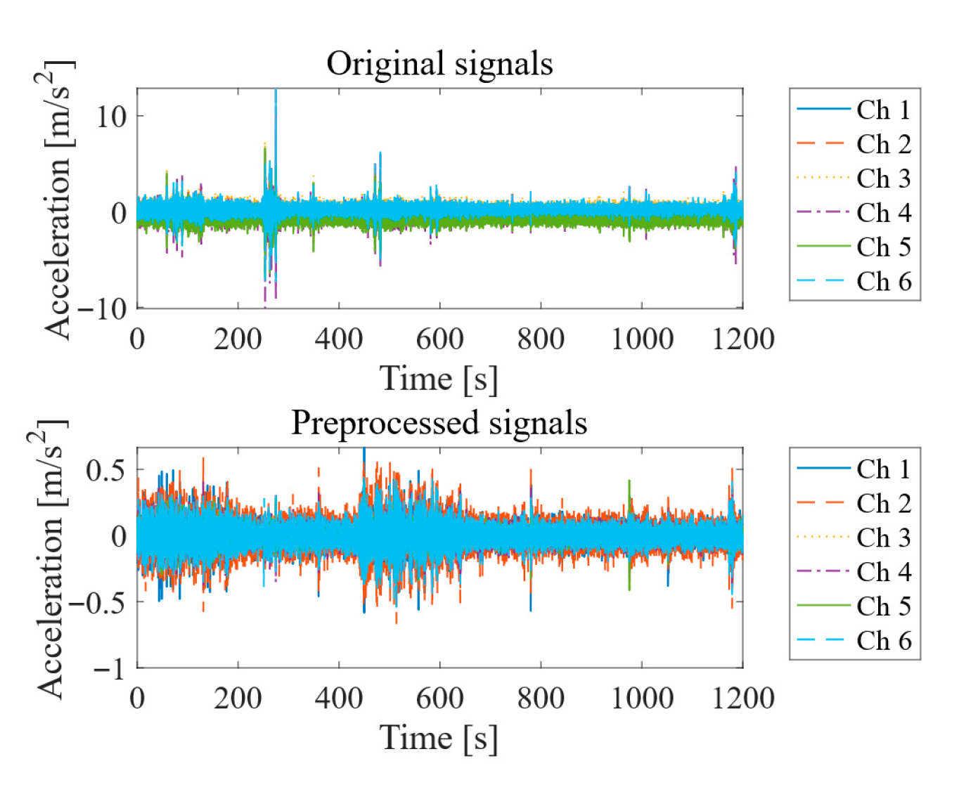
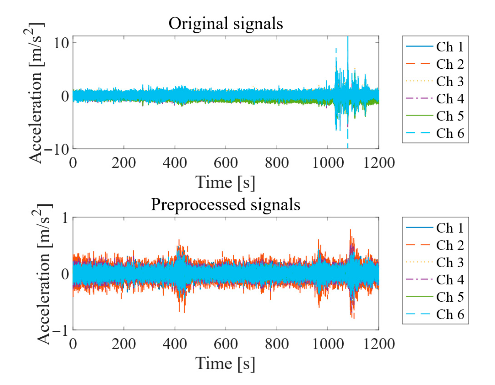
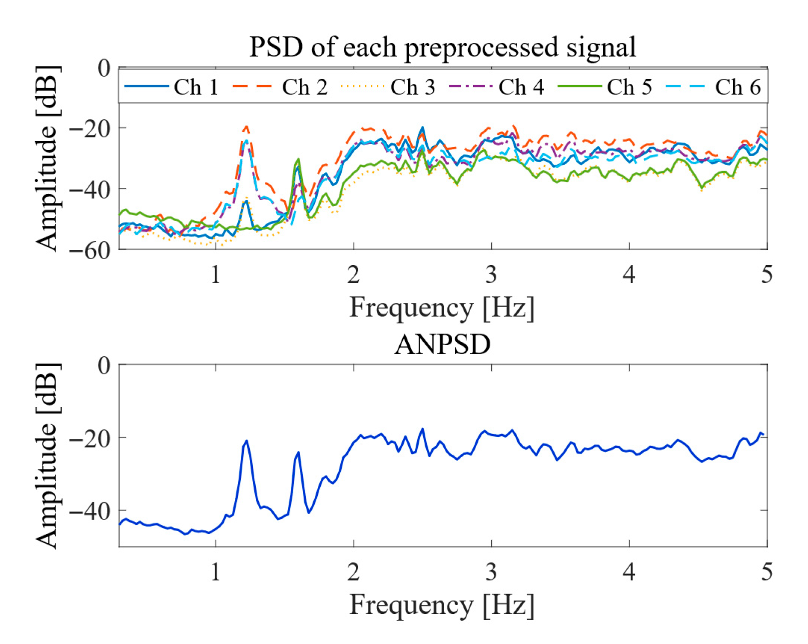
Figure 8 shows the time history of signals collected from Tower A1 before and after preprocessing. In the time domain, the root mean square (RMS) values of the raw signals across six channels ranged from 0.45 to 1.07 m/s² before preprocessing and from 0.05 to 0.11 m/s² after preprocessing. It indicates that vibrations from nearby road traffic and idling trains inside the station were effectively attenuated, bringing the sensor acceleration RMS values across channels to a more uniform level. Figure 9 shows the PSD and ANPSD for each preprocessed channel. The Bode magnitude and phase responses of the fourth-order Butterworth band-pass filter used in signal preprocessing, showing a smooth transition near the cutoff frequencies of 0.3 Hz and 5 Hz (Figure 10). In the frequency domain, the preprocessed signals exhibit clearer spectral peaks near 1.2 Hz, 1.6 Hz, and 2.0 Hz, corresponding to the first few structural modes. It is noteworthy that for the giant A-frame tower structure, the locations available for sensor placement are highly limited (only two vertical cross-sections permit installation). Therefore, this study focuses on the first three identified modes, corresponding to the minimum model order $N_{\min }$ = 2 $n_p$ = 6. Since the primary structural frequencies lie below 5 Hz, the signals were resampled at 32 Hz. The number of block rows for the Toeplitz matrix is determined from Equation (5) as I = $3f_s$/$f_0$ = 79.

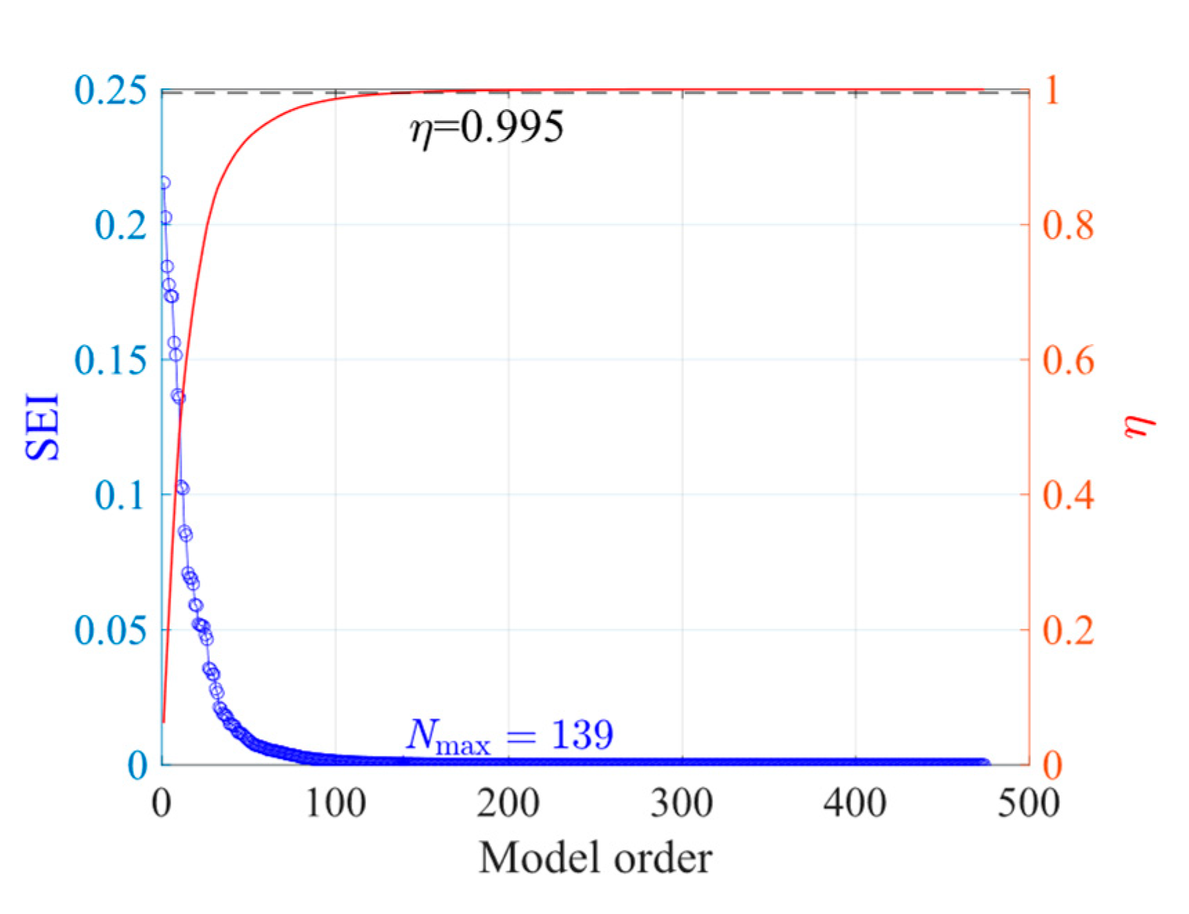
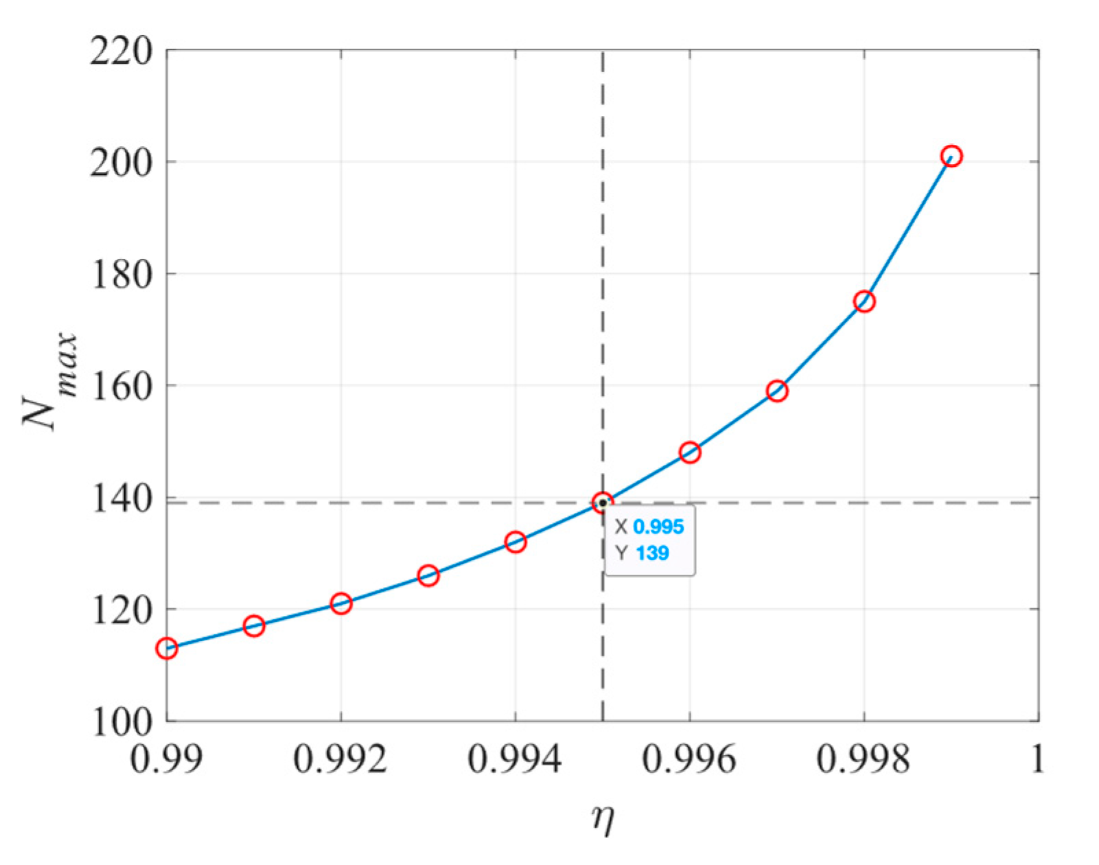
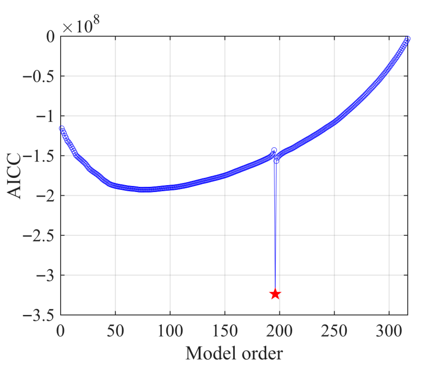
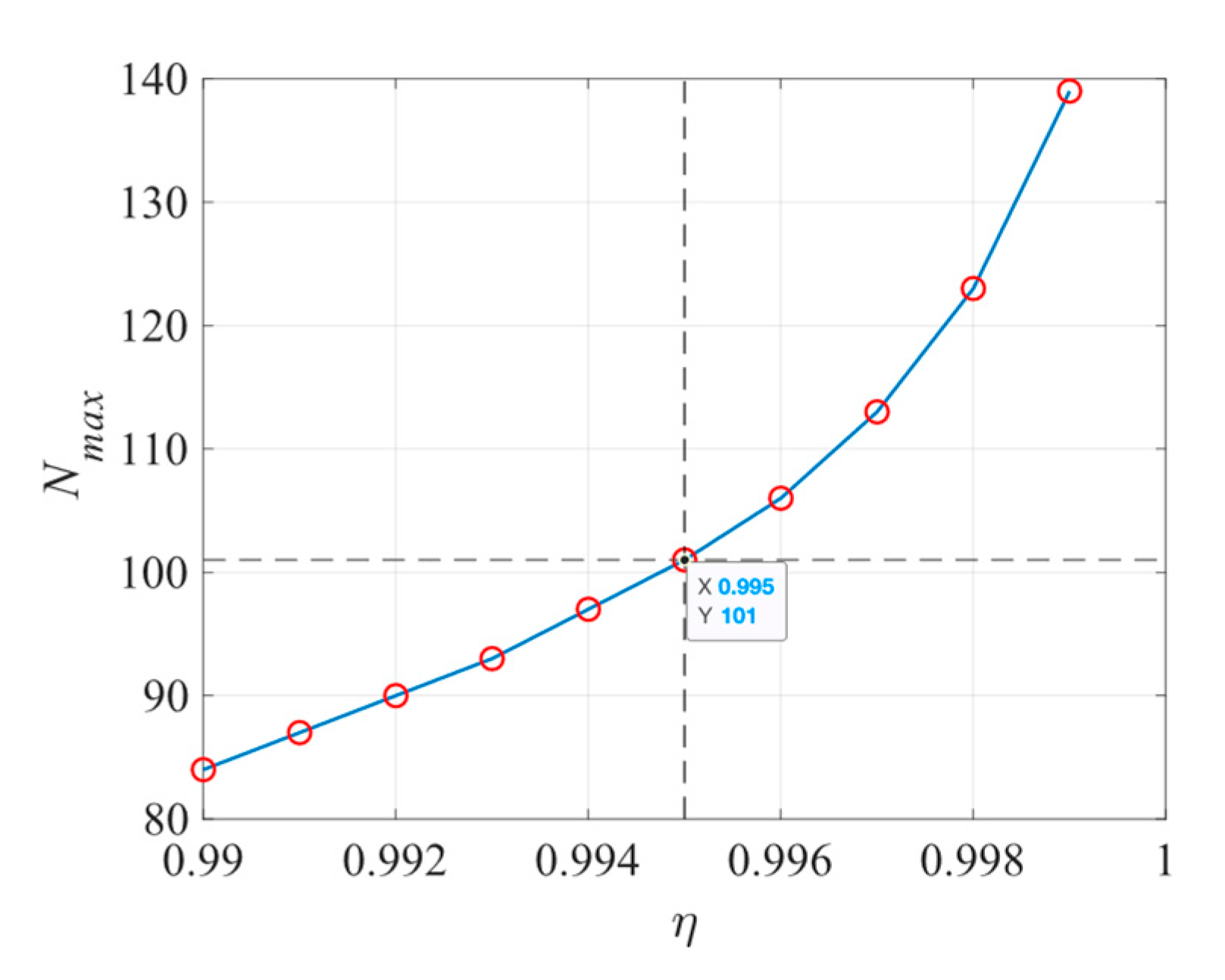
As shown in Figure 11, the AICC automatically determines the maximum model order $N_{\max }$ as 196 (indicated by a red star). For comparison, the variation in SEI and its cumulative contribution with increasing model order is illustrated in Figure 12. Taking a cumulative contribution of 99.5% as an example, the maximum model order estimated by the singular entropy increment method is 139. Further analysis (Figure 13) shows that when the cumulative contribution threshold varies from 99.0% to 99.9% in increments of 0.1%, the automatically determined $N_{\max }$ ranges from 113 to 201. The results indicate that the SEI method yields a maximum model order that is highly sensitive to fluctuations in the cumulative contribution threshold.

Figure 14 presents the stabilization diagram obtained using the covariance-driven SSI method, overlaid with the ANPSD curve. The first three modal poles identified from the stabilization diagram are consistent with the first three spectral peaks of the ANPSD.

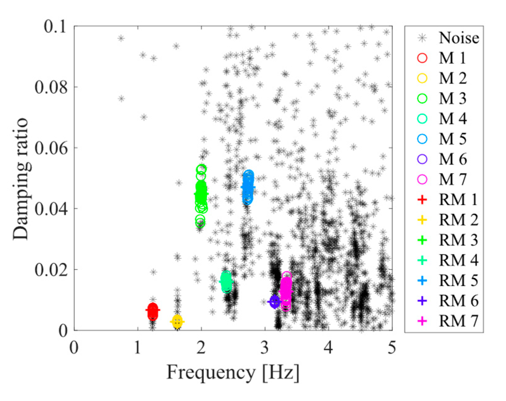
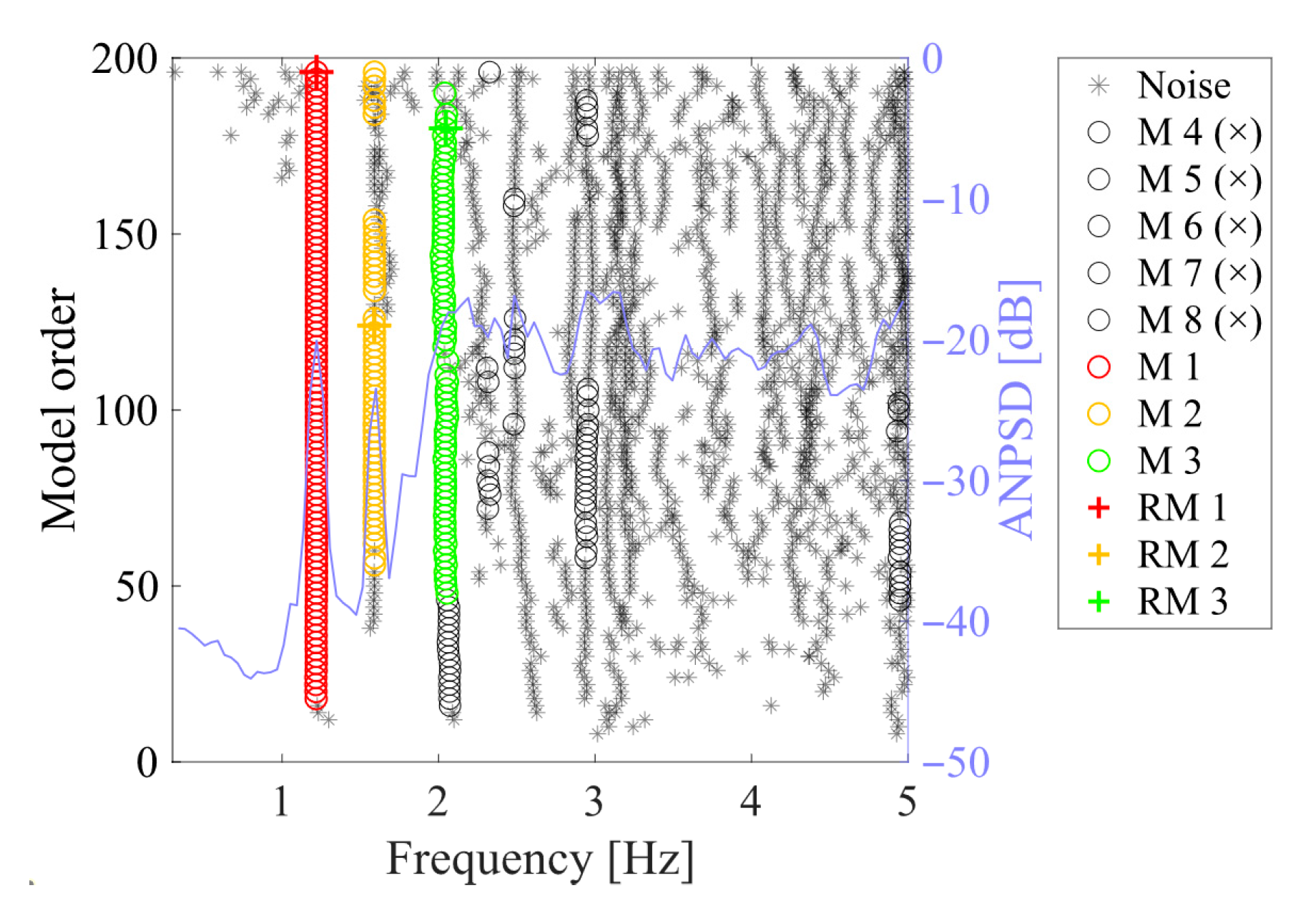
Based on the 1947 modal poles identified in Figure 14, the minimum number of sample points MinPts was set to 8. Then the 8th-nearest modal distance of each pole was calculated from Equations (23)–(25) and arranged in descending order (Figure 15). Finally, the binary K-means clustering method defined in Equation (26) was applied to this distribution, automatically determining the neighborhood radius Eps as 0.295. With these two key parameters (MinPts and Eps) established, the DBSCAN-based automatic modal clustering was performed, as shown in Figure 16. The black background dots correspond to unstable or spurious mathematical modes (noise points), whereas the colored scatter points represent physical structural modes (M1–M7) identified by the clustering algorithm. For each mode order, the representative mode, denoted as RM1–RM7, was indexed by the median damping ratio within the cluster. The results show that at least the first seven modes were successfully identified, with damping ratios exhibiting tight distributions within each cluster. It is demonstrated that the proposed clustering method maintains strong robustness in distinguishing true structural modes under noisy conditions.

It should be noted that only two vertical cross-sections of the large A-shaped tower were available for sensor installation. As a result, higher-order modes could not be clearly distinguished under the limited measurement configuration. Therefore, only the first three modes were included in the statistical evaluation and comparative analysis. Figure 17 further presents the stabilized diagrams of these three modes after automatic clustering. The results indicate that these modes exhibit good convergence and stability across different model orders and that their peak frequencies align closely with the ANPSD spectrum.

Table 2. Frequencies and damping ratios of Tower A1.

Mode Order	Frequency (Hz)	Damping Ratio (%)
1	1.236	0.69
2	1.620	0.28
3	1.998	4.48

and

Table 3. Mode shape coefficients of Tower A1 (westward within the plane or northward out of the plane represents the positive direction).

Test Point	1st	2nd	3rd
#1 (in-plane)	0.030	0.748	−0.474
#2 (out-of-plane)	1.000	−0.218	1.000
#3 (in-plane)	0.013	0.980	−0.217
#4 (out-of-plane)	0.576	−0.177	0.558
#5 (in-plane)	0.017	1.000	−0.214
#6 (out-of-plane)	0.566	−0.240	0.589

list the identified first three modal frequencies, damping ratios, and the corresponding mode-shape coefficients.

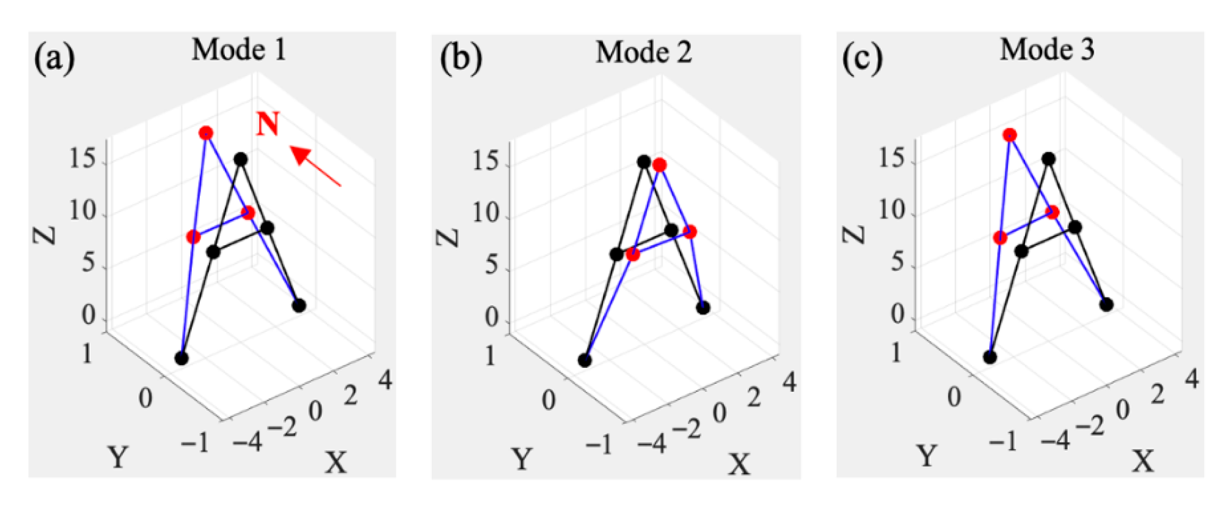
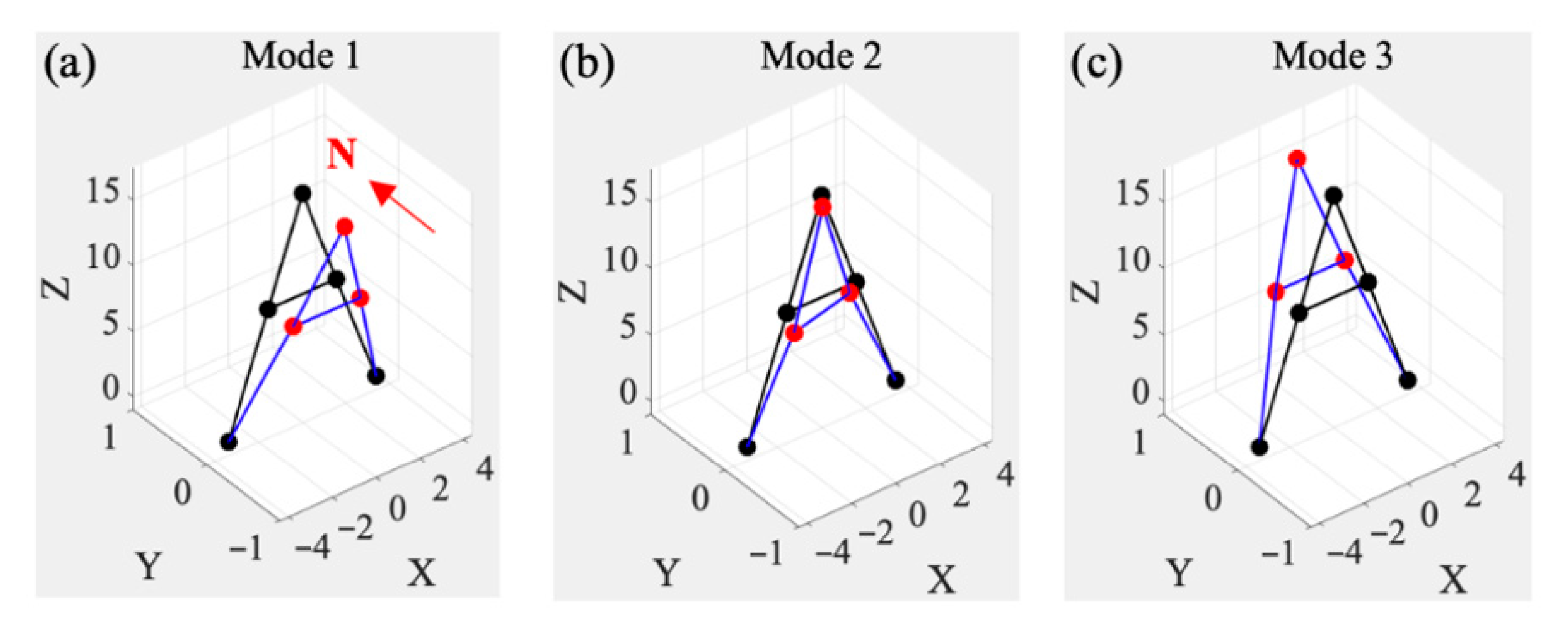
Figure 18 shows the first three spatial mode shapes of Tower A1. (i) The first mode exhibits pure out-of-plane translation (south–north direction, S-N), where the in-plane sensors (#1, #3, #5) have nearly zero mode-shape coefficients, and the maximum amplitude occurs at the tower top (#2). (ii) The second mode is oriented along the northeast–southwest direction (NE-SW) and is dominated by in-plane quasi-translation (#3 and #5), with the maximum amplitude located at the tower beam (#5). (iii) The third mode is oriented along the southwest–northeast direction (SW-NE) and is dominated by out-of-plane quasi-translation (#4 and #6), with the maximum amplitude again at the tower top (#2). In addition, the mode-shape coefficients of the in-plane beam sensors (#3 and #5) remain consistent across all modes, verifying the physical consistency of the measurement points and confirming the accuracy of the identified modal results.

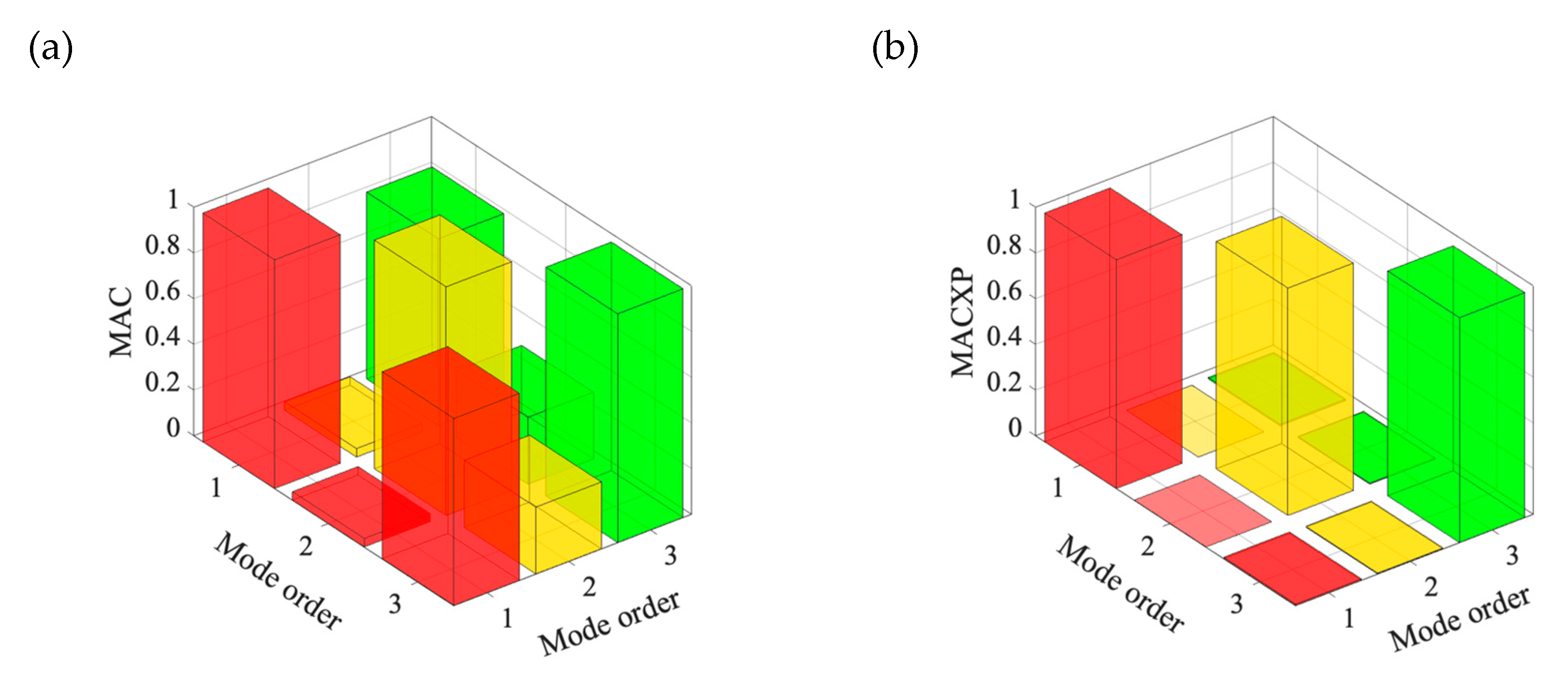
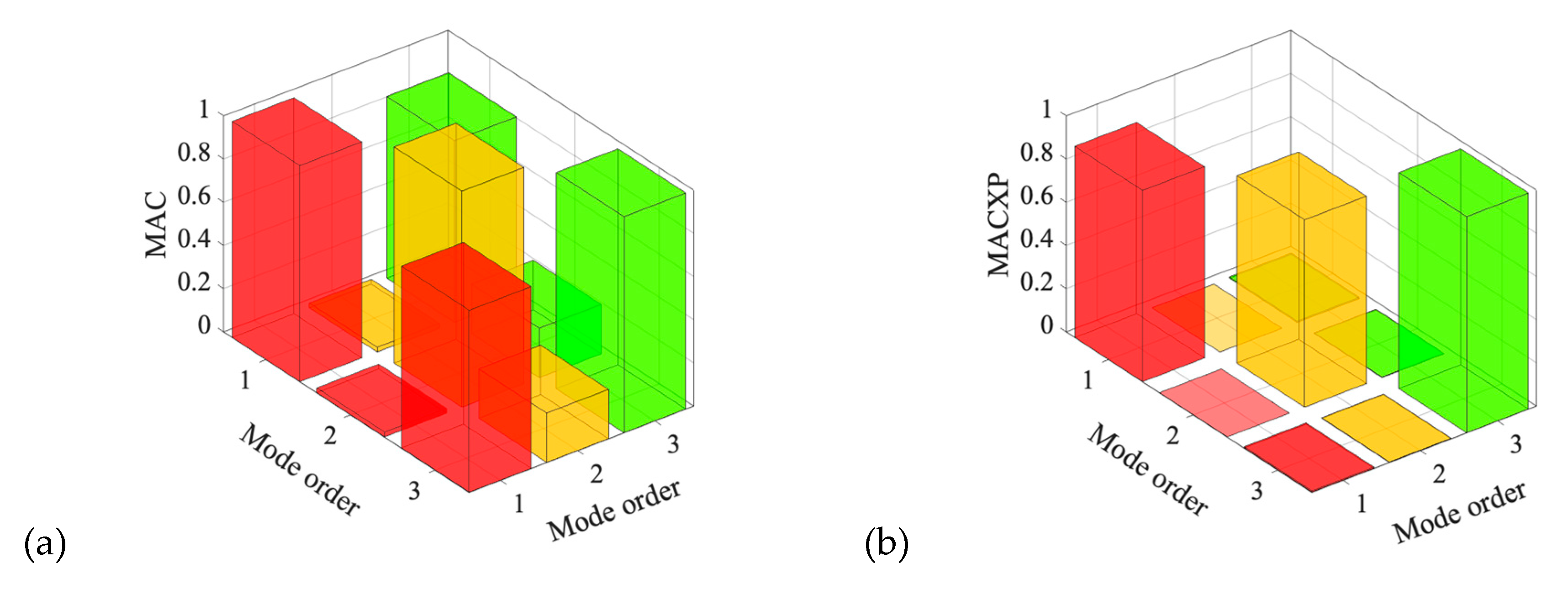
Finally, the identified first three modes were validated using both the Modal Assurance Criterion (MAC) and its extended form, MACXP. In general, a MAC value close to zero indicates low correlation between different modal vectors, which is a necessary condition for assessing modal independence. However, when the measurement layout is limited, spatial aliasing in the modal space is inevitable. In such cases, non-diagonal elements of the MAC matrix can remain large, reducing mode separability. For example, the present results show a high correlation between the first and third modes under the MAC (MAC = 0.82, Figure 19a), indicating significant modal aliasing. Compared with traditional MAC, MACXP captures differences in both phase and complex components between modes, which allows it to overcome the interference caused by limited measurement points (Figure 19b). This highlights the necessity and effectiveness of MACXP for modal validation when sensor placement is constrained.

5.2. Tower A2

Similarly, the results for the signals from Tower A2 in the time domain and frequency domain are shown in Figure 20 and Figure 21, respectively. The RMS values before and after preprocessing range from 0.79–1.69 m/s² and from 0.05–0.12 m/s², respectively. Since the primary structural frequencies lie below 5 Hz, the signals were resampled at 32 Hz. To examine the influence of the Toeplitz matrix block-row number on the AICC, the parameter i was set to 53 according to Equation (5). As shown in Figure 22, the maximum model order automatically determined by the AICC remained 196, showing that the $N_{\max }$ calculated based on AICC is robust against variations in the choice of parameter i under identical test conditions. In contrast, the maximum model order determined using the SEI method increased markedly with higher cumulative contribution ratios, as shown in Figure 23.

The final stabilization diagram obtained from the SSI-Cov method and the first three modes automatically identified through density-based clustering are shown in Figure 24 and Figure 25, respectively. As illustrated, the ANPSD does not exhibit a distinct peak near the third mode around 2.0 Hz, unlike the first two modes. In this case, the time-domain SSI-Cov method demonstrates its robustness in modal identification by forming a stable pole cluster around 2.0 Hz.

The frequencies, damping ratios, and corresponding mode-shape coefficients of the first three modes of Tower A2 are listed in

Table 4. Frequencies and damping ratios of Tower A2.

Mode Order	Frequency (Hz)	Damping Ratio (%)
1	1.220	0.69
2	1.589	0.27
3	2.046	4.81

and

Table 5. Mode shape coefficients of Tower A2 (eastward within the plane or southward out of the plane represents the positive direction).

Test Point	1st	2nd	3rd
#1 (in-plane)	0.053	0.686	0.532
#2 (out-of-plane)	1.000	0.082	1.000
#3 (in-plane)	−0.064	0.939	0.168
#4 (out-of-plane)	0.562	0.356	0.613
#5 (in-plane)	0.004	1.000	0.234
#6 (out-of-plane)	0.587	0.069	0.617

, respectively.

Figure 26 shows the first three spatial mode shapes of Tower A2. (i) The first mode is an out-of-plane pure translation in the north–south direction (N-S) with the maximum amplitude at the tower top (#2). (ii) The second mode is an approximately in-plane translation along the southeast–northwest direction (SE-NW), dominated by in-plane motion and with the maximum amplitude at the west side of the tower beam (#3 and #5); notably, the out-of-plane amplitude at the west side (#4) exceeds that at the east side (#6), causing relative torsion between the two sides and posing a potential risk to the support pin’s anti-slip performance. (iii) The third mode is an out-of-plane translation along the southeast–northwest direction (SE-NW) with the maximum amplitude again at the tower top (#2). Validation of these mode shapes using the extended Modal Assurance Criterion (MACXP) (Figure 27) eliminated the mode-shape aliasing between the first and third modes that remained when the traditional MAC was applied.

5.3. Discussion of the Results

Based on ambient vibration tests conducted on the A-shaped steel towers (A1 and A2), the first three structural modes were identified and compared as follows:

(i)

As summarized in

Table 6. Comparison of frequencies and damping ratios of the two towers.

No.	Tower A1		Tower A2		Differences in Freq. (%)	Differences in Damp. (%)	COMAC
	Freq./ Hz	Damp./(%)	Freq./ Hz	Damp./(%)
1	1.236	0.69	1.220	0.69	1.29	0.56	1.00
2	1.620	0.28	1.589	0.27	1.91	3.18	0.82
3	1.998	4.48	2.046	4.81	2.39	7.34	0.45

, the differences in the first three natural frequencies are small, ranging from 1.29% to 2.39%, while the damping ratios differ by 0.56–7.34%. The cross–orthogonality of the mode shapes (COMAC) for the first three modes is 1.00, 0.82, and 0.45, respectively. These results indicate that the two towers exhibit high consistency in their low-order modes, whereas discrepancies increase progressively in higher-order modes. Such a trend suggests that lower modes primarily reflect the overall structural uniformity, while higher modes are more sensitive to local differences, which is important for structural health monitoring and comparative analysis. It is noted that the third-order mode of Tower A1 is primarily oriented along the southwest–northeast (SW–NE) direction, whereas that of Tower A2 is oriented along the southeast–northwest (SE–NW) direction. These nearly orthogonal modal orientations account for the lower COMAC value (0.45) reported in Table 6.

(ii)

The comparison of the first three mode shapes for Towers A1 and A2 is summarized in

Table 7. Comparison of mode shapes of the two towers.

No.	Tower A1			Tower A2
	Motion	Dominant Direction	Maximum Amplitude	Motion	Dominant Direction	Maximum Amplitude
1	Translation	Out-of-plane (S-N)	Tower top	Translation	Out-of-plane (S-N)	Tower top
2	Quasi-translation	In-plane (NE-SW)	Beam	Quasi-translation	In-plane (SE-NW)	West side of the tower beam
3	Quasi-translation	Out-of-plane (NE-SW)	Tower top	Quasi-translation	Out-of-plane (SE-NW)	Tower top

. Although the overall mode shapes are broadly similar, a notable difference appears in the second mode, which is dominated by in-plane motion. In the reinforced Tower A1, the largest amplitude occurs at the crossbeam, and the out-of-plane components on both sides (#4 and #6 in Table 3) remain essentially consistent, indicating no relative torsion. In contrast, in the unreinforced Tower A2, the second mode shows its maximum amplitude on the west side of the crossbeam, while the out-of-plane components on the two sides (#4 and #6 in Table 5) differ significantly, producing a clear relative torsional response.

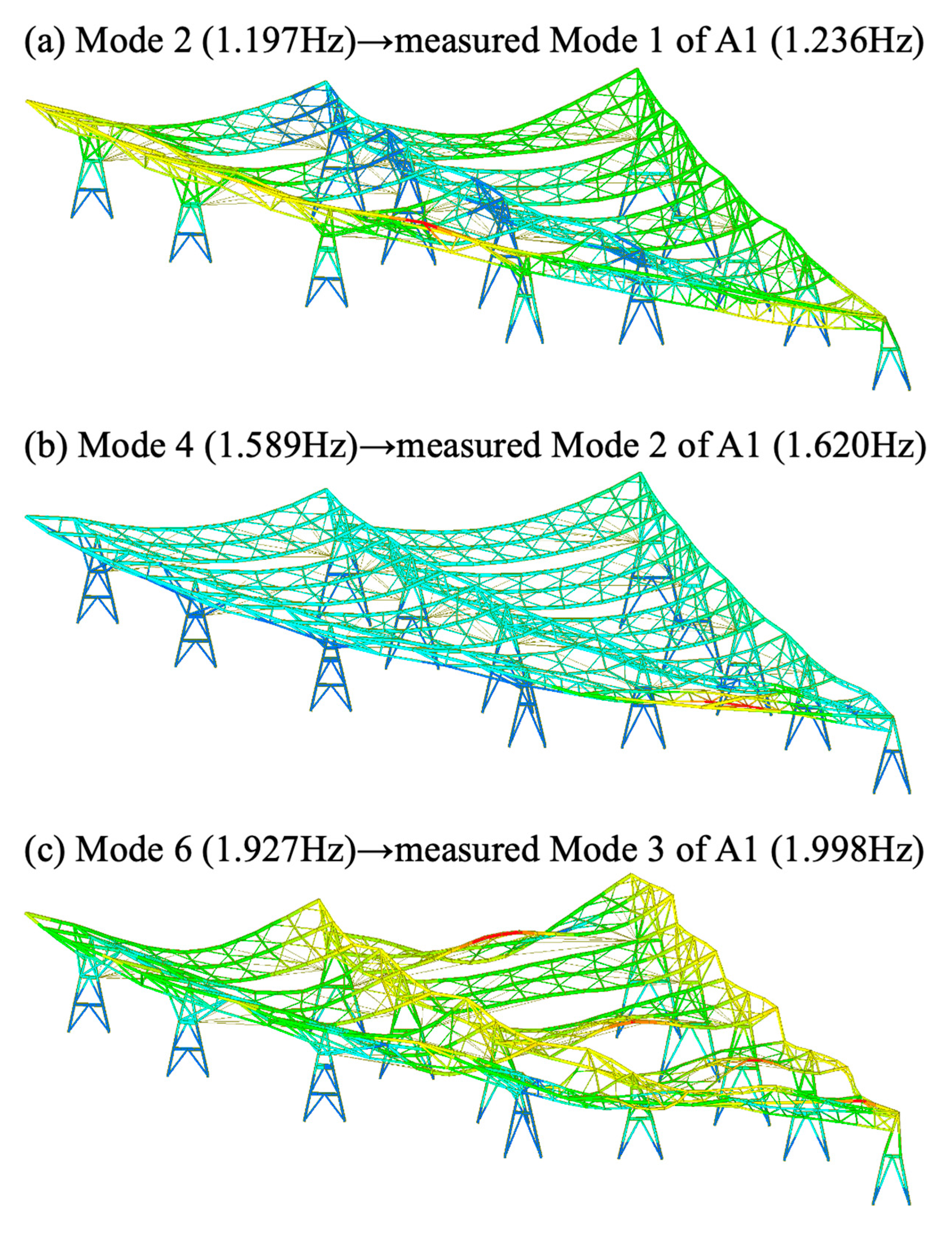
A global FE model was established for canopy Zone 3 to capture the structural interaction between the A-shaped steel towers (A1) and the roof system. Steel members were modeled using beam elements, and the roof panels were represented by shell elements. The primary steel components of the canopy were modeled using Q345 steel, with an elastic modulus of 2.06 × 10¹¹ Pa, a Poisson’s ratio of 0.3, and a density of 7850 kg/m³. Column bases were modeled as hinged supports, and beam-to-column joints were assumed to be rigid. The modal analysis was performed under free-vibration conditions considering only self-weight. The first ten modes of the canopy steel structure in Zone 3 are summarized in

Table 8. Modal results of the finite element model for the overall canopy structure.

Mode	1	2	3	4	5
Freq./Hz	0.997	1.197	1.393	1.589	1.849
Mode	6	7	8	9	10
Freq./Hz	1.927	2.012	2.064	2.205	2.347

, which together contribute more than 95% of the total modal mass participation.

The correspondence between the FE analysis and the measured results of the symmetric A-shaped steel towers (A1) is established based on the similarity of natural frequencies and mode shapes. As illustrated in Figure 28, the first three measured modes of the towers correspond to the 2nd, 4th, and 6th modes of the overall canopy structure. The frequency deviations between the measured and simulated results are 3.16%, 1.89%, and 3.55%, respectively.

6. Conclusions

This study developed an automated modal identification framework based on the corrected Akaike information criterion and adaptive density-based clustering. The proposed framework was validated through field dynamic testing of A-shaped steel towers in a bridge–station-integrated high-speed railway structure under limited sensor configurations. The main conclusions are summarized as follows:

The corrected Akaike information criterion was integrated with covariance-driven stochastic subspace identification to determine the optimal model order. Compared with the traditional singular entropy increment (SEI) method, which is sensitive to threshold selection, the proposed AICC-based approach enables more stable and fully automatic model order estimation, providing a reliable basis for subsequent modal identification.

An adaptive DBSCAN clustering algorithm was employed to distinguish physical modes from spurious ones. A modal distance metric, formulated using the modal assurance criterion extended to the complex modal domain, enhanced mode-shape discrimination under limited measurement conditions. Automatic determination of key parameters in the density-based clustering algorithm further improves robustness and eliminates the need for manual parameter tuning.

The two symmetrical towers exhibited close agreement in frequencies (differences within 2.5%) but more pronounced discrepancies in damping ratios (up to 7.3%), indicating different energy dissipation characteristics. Mode-shape analysis revealed greater divergence at higher orders, particularly in out-of-plane behavior. Notably, the reinforced tower (A1) showed no relative torsional motion in the second mode, whereas the unreinforced tower (A2) exhibited a distinct out-of-plane torsional response, reflecting potential risks related to support pin performance.

References

1. Pan, Y.; Liu, Y.; Huang, C.; Guo, R.; Bao, H.; Shen, L. A review of structural health monitoring of large railway stations. J. Civ. Environ. Eng. 2020, 42, 70–80. [Google Scholar]
2. Du, Y.; Zhang, H.; Liu, B. Consideration on the Current Situation and Development of Structural Health Monitoring of Large Railway Passenger Stations. Railw. Stand. Des. 2023, 67, 1–9. [Google Scholar]
3. Yang, N.; Liu, W.; Bai, F.; Qin, S.; Yu, Y. Durability evaluation of steel structure of platform canopy under corrosion. J. Railw. Sci. Eng. 2020, 17, 181–188. [Google Scholar]
4. Rainieri, C.; Fabbrocino, G. Operational Modal Analysis of Civil Engineering Structures: An Introduction and Guide for Applications; Springer New York: New York, NY, USA, 2014; ISBN 978-1-4939-0766-3. [Google Scholar]
5. Ubertini, F.; Gentile, C.; Materazzi, A.L. Automated Modal Identification in Operational Conditions and Its Application to Bridges. Eng. Struct. 2013, 46, 264–278. [Google Scholar] [CrossRef]
6. Zhou, K.; Li, Q.-S.; Han, X.-L. Modal Identification of Civil Structures via Stochastic Subspace Algorithm with Monte Carlo–Based Stabilization Diagram. J. Struct. Eng. 2022, 148, 04022066. [Google Scholar] [CrossRef]
7. Li, J.; Bao, T.; Ventura, C.E. An Automated Operational Modal Analysis Algorithm and Its Application to Concrete Dams. Mech. Syst. Signal Process. 2022, 168, 108707. [Google Scholar] [CrossRef]
8. Liu, W.; Yang, N.; Bai, F.; Law, S.; Abruzzese, D. An Improved Automated Framework for Operational Modal Analysis with Multi-Stage Clustering and Modal Quality Evaluation. Mech. Syst. Signal Process. 2024, 212, 111235. [Google Scholar] [CrossRef]
9. Van Overschee, P.; De Moor, B.L. Subspace Identification for Linear Systems: Theory—Implementation—Applications; Springer Science & Business Media: Dordrecht, The Netherlands, 2012; ISBN 978-1-4613-0465-4. [Google Scholar]
10. Mostafaei, H.; Ghamami, M. State of the Art in Automated Operational Modal Identification: Algorithms, Applications, and Future Perspectives. Machines 2025, 13, 39. [Google Scholar] [CrossRef]
11. Reynders, E.; Houbrechts, J.; De Roeck, G. Fully Automated (Operational) Modal Analysis. Mech. Syst. Signal Process. 2012, 29, 228–250. [Google Scholar] [CrossRef]
12. Qin, S.; Kang, J.; Wang, Q. Operational Modal Analysis Based on Subspace Algorithm with an Improved Stabilization Diagram Method. Shock Vib. 2016, 2016, 7598965. [Google Scholar] [CrossRef]
13. Zini, G.; Betti, M.; Bartoli, G. A Quality-Based Automated Procedure for Operational Modal Analysis. Mech. Syst. Signal Process. 2022, 164, 108173. [Google Scholar] [CrossRef]
14. Liu, W.; Yang, N.; Liu, B.; Feng, H.; Wang, B.; Du, K.; Abruzzese, D. Sensitivity Analysis and Optimization of User-Defined Parameters in Covariance-Driven Stochastic Subspace Identification. Int. J. Struct. Stab. Dyn. 2025, 2650202. [Google Scholar] [CrossRef]
15. Teng, J.; Tang, D.-H.; Zhang, X.; Hu, W.-H.; Said, S.; Rohrmann, R. Automated Modal Analysis for Tracking Structural Change during Construction and Operation Phases. Sensors 2019, 19, 927. [Google Scholar] [CrossRef]
16. Pourgholi, M.; Mohammadzadeh Gilarlue, M.; Vahdaini, T.; Azarbonyad, M. Influence of Hankel Matrix Dimension on System Identification of Structures Using Stochastic Subspace Algorithms. Mech. Syst. Signal Process. 2023, 186, 109893. [Google Scholar] [CrossRef]
17. Zhang, X.; Li, D.; Song, G. Structure Damage Identification Based on Regularized ARMA Time Series Model under Environmental Excitation. Vibration 2018, 1, 138–156. [Google Scholar] [CrossRef]
18. Yaghoubi, V.; Vakilzadeh, M.K.; Abrahamsson, T.J.S. Automated Modal Parameter Estimation Using Correlation Analysis and Bootstrap Sampling. Mech. Syst. Signal Process. 2018, 100, 289–310. [Google Scholar] [CrossRef]
19. He, M.; Liang, P.; Zhang, Y.; Yang, F.; Liu, J. Unified Method for Fully Automated Modal Identification and Tracking with Consideration of Sensor Deployment. Eng. Struct. 2022, 260, 114223. [Google Scholar] [CrossRef]
20. Vacher, P.; Jacquier, B.; Bucharles, A. Extensions of the MAC Criterion to Complex Modes. In Proceedings of the International Conference on Noise and Vibration Engineering, Leuven, Belgium, 20–22 September 2010; pp. 2713–2726. [Google Scholar]
21. Bhusal, U.; Tezcan, J. Automatic Density-Based Clustering for Operational Modal Analysis. Nat. Hazards Rev. 2025, 26, 04025004. [Google Scholar] [CrossRef]
22. Ester, M.; Kriegel, H.-P.; Sander, J.; Xu, X. A Density-Based Algorithm for Discovering Clusters in Large Spatial Databases with Noise. In Proceedings of the KDD, Portland, OR, USA, 2–4 August 1996; Volume 96, pp. 226–231. [Google Scholar]
23. Ye, C.; Zhao, X. Automated Operational Modal Analysis Based on DBSCAN Clustering. In Proceedings of the 2020 International Conference on Intelligent Transportation, Big Data & Smart City (ICITBS), Vientiane, Laos, 11–12 January 2020; pp. 864–869. [Google Scholar]
24. Boroschek, R.L.; Bilbao, J.A. Interpretation of Stabilization Diagrams Using Density-Based Clustering Algorithm. Eng. Struct. 2019, 178, 245–257. [Google Scholar] [CrossRef]
25. Civera, M.; Sibille, L.; Zanotti Fragonara, L.; Ceravolo, R. A DBSCAN-Based Automated Operational Modal Analysis Algorithm for Bridge Monitoring. Measurement 2023, 208, 112451. [Google Scholar] [CrossRef]
26. Bendat, J.S.; Piersol, A.G. Random Data: Analysis and Measurement Procedures; John Wiley & Sons: Hoboken, NJ, USA, 2011; ISBN 978-1-118-21082-6. [Google Scholar]
27. Xia, X. The Comparison of Modal Analysis Methods Under Ambient Vibration. Master’s Thesis, Central South University, Changsha, China, 2013. [Google Scholar]
28. Liu, W.; Yang, N.; Bai, F.; Chang, P. Parameter Optimization of Covariance-driven Stochastic Subspace Identification Method Based on Sensitivity Analysis. Eng. Mech. 2021, 38, 157–167. [Google Scholar]
29. Zeng, J.; Hu, Z. Automated Operational Modal Analysis Using Variational Gaussian Mixture Model. Eng. Struct. 2022, 273, 115139. [Google Scholar] [CrossRef]
30. Liu, W.; Yang, N.; Law, S.S.; Abruzzese, D.; Bai, F.; Cao, X. Automated Operational Modal Analysis with Adaptive DBSCAN-based Algorithm and Its Engineering Application. J. Civ. Struct. Health Monit. 2025. accepted. [Google Scholar] [CrossRef]
31. Magalhães, F.; Cunha, Á.; Caetano, E. Online Automatic Identification of the Modal Parameters of a Long Span Arch Bridge. Mech. Syst. Signal Process. 2009, 23, 316–329. [Google Scholar] [CrossRef]
32. Tronci, E.M.; De Angelis, M.; Betti, R.; Altomare, V. Multi-Stage Semi-Automated Methodology for Modal Parameters Estimation Adopting Parametric System Identification Algorithms. Mech. Syst. Signal Process. 2022, 165, 108317. [Google Scholar] [CrossRef]
Figure 1. Section of the railway passenger station.
Buildings 15 03754 g001
Figure 2. Plan of the railway passenger station.
Buildings 15 03754 g002
Figure 3. Steel structure system of the canopy: (a) canopy zones 1 and 3; (b) canopy zone 2.
Buildings 15 03754 g003
Figure 4. Support of steel Tower A1: (a) pin slippage and cover plate detachment (pre-repair); (b) steel plate positioning treatment (post-repair).
Buildings 15 03754 g004
Figure 5. Sensor arrangement scheme: (a) aerial work platform; (b) schematic diagram of test point layout; (c) accelerometer.
Buildings 15 03754 g005
Figure 6. Flowchart of structural dynamic characteristic identification.
Buildings 15 03754 g006
Figure 7. Schematic diagram of modal aliasing under limited sensor configuration.
Buildings 15 03754 g007
Figure 8. Raw signal from Tower A1 and its preprocessing.
Buildings 15 03754 g008
Figure 9. PSD and ANPSD of Tower A1.
Buildings 15 03754 g009
Figure 10. Bode diagram of fourth-order Butterworth filter.
Buildings 15 03754 g010
Figure 11. AICC-based model order determination.
Buildings 15 03754 g011
Figure 12. SEI-based model order determination.
Buildings 15 03754 g012
Figure 13. Perturbation analysis of cumulative contribution rate on N max .
Buildings 15 03754 g013
Figure 14. Stabilization diagram of Tower A1.
Buildings 15 03754 g014
Figure 15. Adaptive determination of Eps.
Buildings 15 03754 g015
Figure 16. Results of automatic modal clustering.
Buildings 15 03754 g016
Figure 17. Stabilization diagram of the first three modes in automatic clustering.
Buildings 15 03754 g017
Figure 18. The first three orders of mode shapes of Tower A1.
Buildings 15 03754 g018
Figure 19. Verification of mode shapes: (a) MAC; (b) MACXP.
Buildings 15 03754 g019
Figure 20. Raw signal from Tower A2 and its preprocessing.
Buildings 15 03754 g020
Figure 21. PSD and ANPSD of Tower A2.
Buildings 15 03754 g021
Figure 22. AICC-based model order determination (Tower A2).
Buildings 15 03754 g022
Figure 23. Perturbation analysis of cumulative contribution rate on N max (Tower A2).
Buildings 15 03754 g023
Figure 24. Results of automatic modal clustering (Tower A2).
Buildings 15 03754 g024
Figure 25. Stabilization diagram of the first three modes in automatic clustering (Tower A2).
Buildings 15 03754 g025
Figure 26. The first three orders of mode shapes of Tower A2.
Buildings 15 03754 g026
Figure 27. Verification of mode shapes (Tower A2): (a) MAC; (b) MACXP.
Buildings 15 03754 g027
Figure 28. Modal analysis of the canopy finite element model and its correspondence with the measured modes.
Buildings 15 03754 g028