1. Introduction
Structural health monitoring (SHM) offers significant benefits for bridges and road infrastructure, enhancing their safety, durability, and maintenance efficiency [
1,
2,
3,
4]. SHM helps optimise maintenance schedules, reducing unnecessary inspections and focusing resources on areas that require immediate attention [
5,
6]. It not only extends the lifespan of the bridges but also minimises downtime and maintenance costs. Furthermore, SHM provides valuable data that can be used to improve the design and construction of future bridges, ensuring they are more resilient to environmental stresses and usage demands [
7,
8].
SHM systems are applied to most large bridges. The SHM system supports managers and related units in monitoring and evaluating the condition of bridge structures. Recently, with the rapid advancement of sensor technologies and the processing capabilities of computers, SHM systems have become increasingly efficient and reliable. Progress in sensor technology has enabled the collection of detailed and continuous data from infrastructure projects, providing precise information about the condition and performance of structures. Sensors such as fibre Bragg grating (FBG) accelerometers, strain gauges, or linear variable differential transformers (LVDTs) are installed at optimal locations on the structure [
9,
10,
11]. Based on the data collected from the above sensors, humans can analyse and evaluate structural abnormalities [
12,
13,
14]. Sensor-collected time-series data contains a lot of information that helps experts predict damage conditions [
15,
16]. The development of signal processing and data analysis technologies, particularly artificial intelligence (AI) and machine learning, has optimised the process of analysis and decision-making in SHM systems [
17]. ML models are widely applied to process and analyse complex sensor data. It enhances the ability to detect and predict structural damage, thereby improving reliability and extending the lifespan of infrastructure [
18]. Moreover, advancements in computer systems and software have facilitated the processing of big data and real-time analysis. Modern SHM systems can integrate deep learning algorithms to continuously analyse sensor data, enabling the early detection of abnormal changes in structures, thereby minimising risks and maintenance costs [
12]. These advancements have opened new avenues for monitoring, maintaining, and managing large infrastructure projects such as bridges, dams, and key transportation structures, contributing to enhanced safety and operational efficiency. To achieve these accomplishments, data collected from sensors plays an extremely important role. The quality, continuity, and accuracy of sensor data are the key factors that determine the success of the SHM system.
However, failure to ensure data quality in experiments or SHM systems is a frequent occurrence. Data may be lost, interrupted, or severely corrupted. This problem directly affects the monitoring results. The results may not be accurate, incorrect, or misleading, affecting the structural monitoring process [
19,
20,
21]. There are many causes of data loss or poor-quality data. Sensors operate under the influence of load and are affected by many other environmental factors: rain, wind, and humidity. They may be damaged or have other problems related to ageing [
22,
23]. For wired signal transmission systems, the signal may be faulty due to broken or short-circuited signal cables. Wireless health monitoring systems also frequently face signal loss due to weak transmission between transmitters. In general, data loss in SHM systems has many causes and is unavoidable. Identifying errors in the SHM system, such as those caused by sensor malfunctions, transmission system issues, or software management errors, is a time-consuming and challenging task. If the cause and location of the error are found, replacement or repair solutions will not ensure the system’s data quality due to inconsistency. It drives the need for another solution to reconstruct lost or corrupted data.
Investigating data reconstruction methods in SHM is very important regarding the safety and sustainability of critical infrastructure and buildings. SHM utilises sensor systems to continuously collect data on the structural state, enabling the analysis and prediction of potential damage.
Furthermore, data reconstruction is crucial for providing accurate information at the lifecycle level for digital twinning purposes. Several studies have already highlighted the majority of advantages associated with digital twin applications, which support the creation of analytical and predictive models, as well as strategic decision-making in infrastructure management and operation [
24,
25].
Intelligent algorithms and artificial intelligence (AI) have been popular in recent years as solutions to numerous data reconstruction issues [
26,
27,
28]. Artificial intelligence (AI) models can automatically forecast and restore missing or noisy data by learning from past data trends [
29,
30]. The prominent advantages of AI in SHM data reconstruction include the automation and optimisation of the monitoring process, minimising human intervention and enhancing data reliability. Moreover, AI can adapt to changes and anomalies in the data, improving the effectiveness of detecting and preventing structural issues. In the context of increasingly advanced SHM technology, AI enhances monitoring quality and opens up new opportunities for managing and maintaining complex structural systems [
30]. In the framework of Bayesian multi-task learning using multidimensional Gaussian programming, Wan and Ni [
31] suggested a technique to recover SHM data. The reconstruction performance that was attained is very dependable. Zhang and Luo [
32] recovered missing stress data by using data correlation. The interpolation error using this method is approximately 5–7%. Other studies have also proposed data recovery techniques that yield extremely accurate results [
33,
34,
35].
In the field of SHM, many researchers have started to reconstruct data from deep learning models. To restore lost data in SHM, Lei et al. [
9] employed deep convolutional generative adversarial networks. In practice, the suggested deep learning architecture performs well and can recreate accelerometer and strain sensor data on models. Jiang et al. [
20] used an unsupervised learning technique based on a generative adversarial network to retrieve partial data from a long-term health monitoring system. The method of reconstructing SHM data using convolutional neural networks was first presented by Fan et al. [
36]. Even for signals with extreme data loss rates of up to 90%, our technique enables exceptional lost data recovery. In their study, Fan et al. [
37] used highly linked convolutional networks to reconstruct dynamic responses with good results. Additionally, numerous studies [
35,
36] employ deep learning in data reconstruction. The proposed methods all achieve significant success in reconstructing different types of data [
38,
39,
40].
Recent studies have increasingly applied long short-term memory (LSTM) networks for time-series data reconstruction due to their ability to capture long-range dependencies and nonlinear dynamics [
41]. In the field of structural monitoring, LSTM models have been explored for imputing missing acceleration or strain signals when sensor malfunctions occur. Several works demonstrated that LSTM-based models can effectively recover dynamic response histories while preserving modal characteristics, even under high missing-data ratios [
42]. Beyond civil engineering, LSTM networks have also been employed in environmental monitoring, energy systems, and biomedical signals to reconstruct incomplete datasets, further highlighting their versatility and robustness [
43]. These studies collectively indicate that LSTM is well-suited for reconstructing vibration data in structural health monitoring (SHM), providing both accurate temporal recovery and fidelity in the frequency domain [
44].
In this study, an LSTM network is used to reconstruct data from accelerometers for SHM. The LSTM architecture is particularly well-suited for this task because of its ability to capture temporal dependencies in sequential data, making it effective in modelling the dynamic responses of structures under varying conditions. By leveraging the LSTM’s capacity to learn from historical patterns in the data, the proposed approach enables accurate reconstruction of corrupted or incomplete signals. This not only improves the quality of the input data but also enhances the performance of subsequent SHM processes, such as damage detection and condition assessment. The study addresses the following research questions: (i) How effectively can an LSTM-based model reconstruct missing acceleration data under different patterns of data loss? (ii) Does a multichannel LSTM architecture significantly improve reconstruction accuracy compared with single-channel models and conventional interpolation approaches? (iii) Can the reconstructed signals preserve essential dynamic characteristics of the bridge, such as modal frequencies and spectral features, that are critical for SHM applications? (iv) What are the main limitations and potential improvements when applying deep-learning-based data reconstruction to real-world SHM practice?
The novelty and contributions of this study are threefold. First, previous studies mainly deal with randomly missing data or small-scale test structures. This study addresses system sensor error in the context of operational bridge monitoring, bringing the problem closer to real-life SHM conditions. Second, existing literature typically only addresses small, uncomplicated data loss scenarios. This study, on the other hand, addresses the problem in a more general way. Data reconstruction will be performed in the single-channel case, and the more difficult multi-channel loss scenarios with two and three missing sensors will be analysed. Finally, a comprehensive quantitative evaluation of the reconstructed signals is provided, utilising multiple error measures. Additionally, a direct comparison between LSTM and classical RNN baselines is conducted. These contributions demonstrate both the novelty and practicality of this study. The study provides insights for sensor placement and contingency planning in practical SHM applications.
2. Methodology
2.1. Long Short-Term Memory (LSTM)
Particularly useful for tasks where the order of inputs counts, such as time-series analysis, language modelling, and speech recognition, recurrent neural networks (RNNs) [
45], a specialised kind of artificial neural network designed to handle sequential data. Unlike traditional feedforward neural networks, RNNs have directed cycle connections, enabling them to retain a ‘memory’ of prior inputs through their hidden state. This recurrent mechanism enables RNNs to process sequences of variable length and capture temporal dependencies. The hidden state at each time step
t is computed based on the input at time
t and the hidden state from the previous time step
t − 1, typically using the formula [
46]:
where
and
represent weight matrices,
represents a bias vector, and
is an activation function such as tanh or ReLU.
Despite their powerful ability to handle sequential data, RNNs have several notable drawbacks. One of the primary issues is the vanishing gradient problem, where gradients used in backpropagation through time become exceedingly small, causing the network to learn very slowly or even stop learning entirely as it struggles to adjust weights effectively. These limitations reduce the effectiveness of RNNs in tasks that require long-term context and stable learning dynamics, necessitating more advanced architectures, such as LSTM networks.
LSTM [
47] networks are a specialised type of RNNs designed to address the shortcomings of traditional RNNs, particularly the vanishing gradient problem. In order to control the information flow, LSTM networks introduce a novel architecture that consists of memory cells and an input, forget, and output gate mechanism. These gates allow LSTM networks to maintain and selectively update information over long periods, effectively capturing long-term dependencies in sequential data. The input gate regulates the influx of new information into the cell state, the forget gate decides which information to discard from the cell state, and the output gate manages the information transmitted to the subsequent hidden state. The ability of LSTMs to remember important information over extended periods significantly enhances their performance and stability compared to traditional RNNs, providing a robust solution for complex sequential tasks. Some studies have shown that, in most cases, LSTM is much more effective than RNN [
45,
48,
49].
Input gate—The task of this gate is to detect values for memory modifications. The Sigmoid function determines which values to classify as either 0 or 1. The tanh function assigns weights to the passed values, determining how important they are between −1 and 1 [
50].
Forget gate—This gate detects parts that need to be removed from the block. By looking at the previous state
, input and return a value between 0 (remove this value) and 1 (keep this value) for each number in cell state
.
Output gate—At this stage, the output is calculated based on the input and the block’s memory. The values converted to 0 or 1 are controlled and determined by the Sigmoid function. The Tanh function allows for deciding which value to pass: 0 or 1. The tanh function assigns weights to the passed values, determining their importance within the range of −1 to 1, and then multiplies the output by a sigmoid.
While the above equations describe the generic operation of LSTMs, their specific advantages become clearer in the context of bridge SHM. Vibration responses of large-span bridges are typically long, noisy, and influenced by multiple loading sources such as traffic and wind. Missing segments from accelerometers further complicate the signals, often introducing discontinuities that degrade modal identification. LSTMs are particularly valuable here because they can (i) capture long-term temporal dependencies inherent in structural vibration records, (ii) learn cross-channel relationships when multiple sensors are deployed along the bridge, and (iii) reconstruct continuous acceleration histories that preserve dynamic characteristics such as natural frequencies and mode shapes. These capabilities make LSTMs more suitable than simple interpolation or traditional time-series models for reconstructing missing SHM data and ensuring reliable condition assessment of bridges.
2.2. Data Pre-Processing
The data pre-processing stage is crucial in preparing data for training in an LSTM network, especially when the input consists of time-series data. This process involves several key steps to ensure that the data is appropriately formatted and optimised for the LSTM model. Firstly, the raw time-series data is typically collected from sensors or other sources. Next, the data is often normalised or scaled to a consistent range. By ensuring that all features are on the same scale, normalisation keeps some features from taking over the training process because of their greater magnitudes. This step helps improve the convergence of the LSTM model during training and enhances its overall performance.
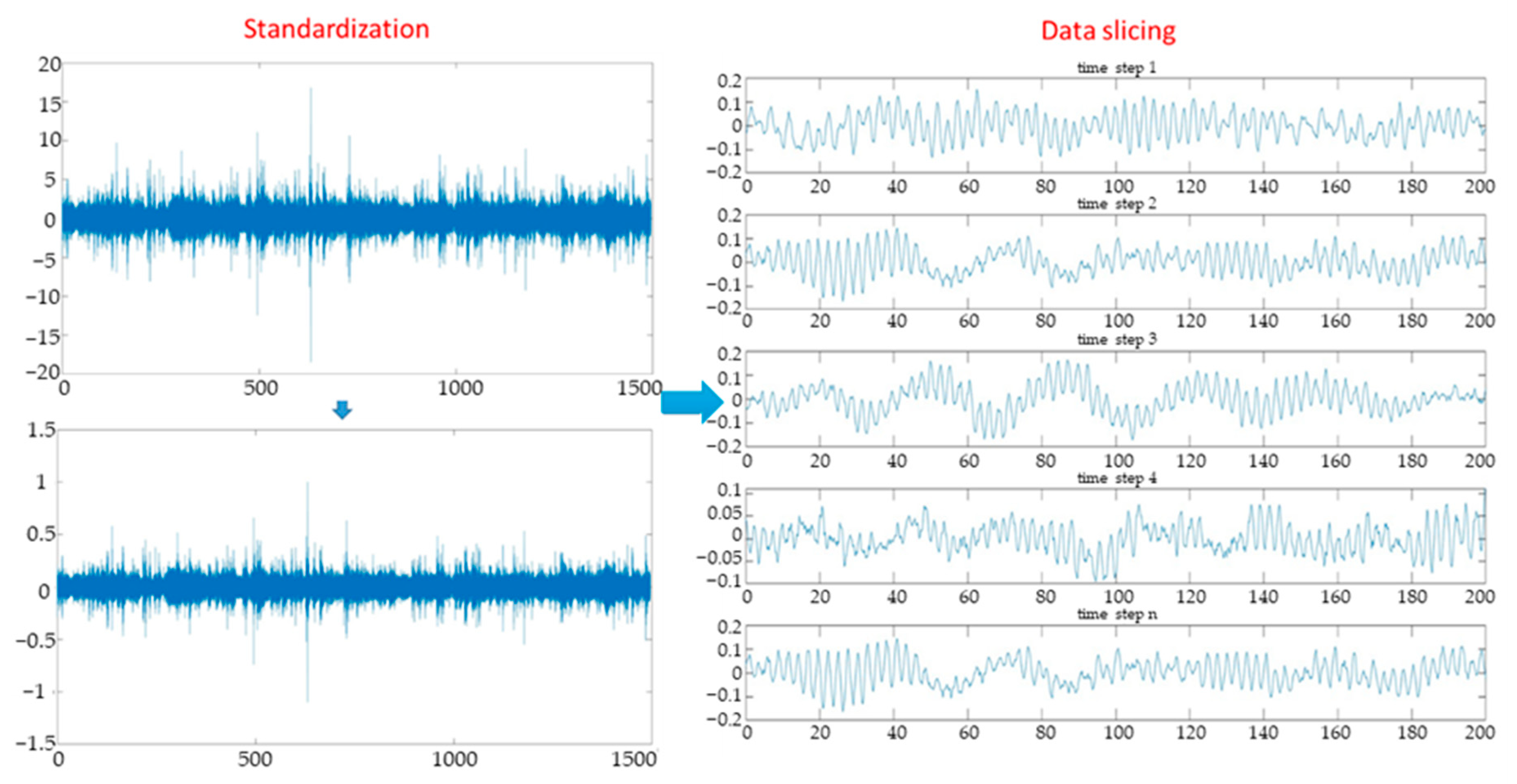
After normalisation, the data is typically segmented into sequences or windows, each representing a time step in the time series. This segmentation allows the LSTM model to learn temporal patterns and dependencies within the data. The size of these sequences or windows is a crucial hyperparameter that can be adjusted based on the specific characteristics of the data and the model’s requirements.
Furthermore, feature engineering may be employed to extract relevant features from the time-series data. These features could include statistical measures such as mean, standard deviation, or trend analysis, as well as domain-specific features that capture important characteristics of the data relevant to the problem at hand.
After pre-processing, the data is divided into training, validation, and testing sets. The LSTM model is trained using the training set; hyperparameters are fine-tuned, and the model’s performance is tracked during training using the validation set; and the final performance of the trained model on unseen data is evaluated using the testing set. In summary, the data pre-processing stage for training an LSTM model on time-series data involves cleaning, normalisation, segmentation, feature engineering, and dataset splitting. By carefully pre-processing the data, the LSTM model learns effectively from the time-series data and achieves optimal performance for the given task.
In this study, data from sensors in the monitoring system are used to train the LSTM. Data obtained from the sensors will be set to correspond to the sensitivities of each sensor in the measurement programme. These values will not have the same standard. Standardisation of data aims to bring all sensor data to the same value range, from 0 to 1. Implementing the following equation on the dataset from the sensors, standardised data will be obtained [
51]:
where
is the data before standardisation;
is standardised data;
is the average value;
is the variance.
In prior studies [
51], sequence lengths on the order of a few hundred samples have often been reported to provide a reasonable balance between capturing long-term temporal dependencies and maintaining computational efficiency. In this work, we empirically observed that window sizes of 200–400 samples yielded stable and accurate reconstructions for our dataset, which was collected at a sampling rate of 1651 Hz. It should be noted that the optimal sequence length is not universal. Factors such as sampling rate, structural dynamic properties, and sensor configuration can significantly influence the choice of window size. The present finding, therefore, reflects both insights from the literature and validation against the characteristics of the bridge case study considered here. Data obtained from
n sensors will be processed and divided into segments of 200 samples each. Specifically, data will be returned in the form of
n × 200 × time steps.
Figure 1 shows the data preparation process:
2.3. Post-Processing: Data Reconstruction
The training process commences after the data has been pre-processed and prepared. Sensor data often manifests as a continuous time series, thus necessitating subdivision into smaller data samples that LSTM networks can understand and process. It is typically achieved by segmenting the data into fixed-length sliding windows, each window representing a fixed time interval within the data. Once the data has been segmented into time series, an LSTM network is constructed and trained on the segmented data. This process is usually conducted using the backpropagation algorithm, where the parameters of the LSTM network are gradually adjusted to minimise the error between predictions and the actual values of the data. To ensure the model’s generalizability, performance evaluation methods such as cross-validation or separate testing datasets are typically employed. It allows assessment of whether the model can effectively predict new data, rather than just performing well on the training data. Finally, once the model has been adequately trained, it can be deployed for sensor data reconstruction in real-world scenarios.
The input and output of the LSTM network are determined. The input here is data from standard sensors. The output is the sensors’ data, which is assumed to be in error. The input data will be in the form of m × 200 × time steps (m is the number of standard sensors), and the output data will be in the form of q × 200 × time steps (q is the number of error sensors, requiring data reconstruction).
After dividing the dataset, the training set is first used to train the LSTM so that the network can learn the nonlinear mapping relationship between the standard sensor and the corrupted sensor data. Once the network training is complete, the test set is fed into the trained neural network to reconstruct the lost data.
Figure 2 shows the input and output of the network after training in the general case.
3. Case Study
In this study, a case study was conducted at the Lac Quan Bridge, a large bridge (
Figure 3). The bridge has a design load capacity of H30-XB80. The span configuration consists of 33 × 4 + 55 + 90 + 55 + 33 × 5 m, with an overall length of 503.67 m and a total span length of 497 m. The bridge spans the Ninh Co River, allowing boats below to pass through with a clearance width of up to 11 m. Constructed using the balanced cantilever method, which was one of the most modern methods at the time, the bridge holds significant importance in facilitating trade among neighbouring districts, serving as an economic lifeline for the entire province.
The superstructure of the bridge has a total width of 11 m, with the approach spans comprising 9 prestressed concrete spans with a T-shaped cross-section, and the main span being a prestressed concrete box girder. The substructure includes abutments with goat-leg-shaped supports made of reinforced concrete, column-type piers for the approach spans, and solid heavy piers for the main span.
3.1. Data Acquisition
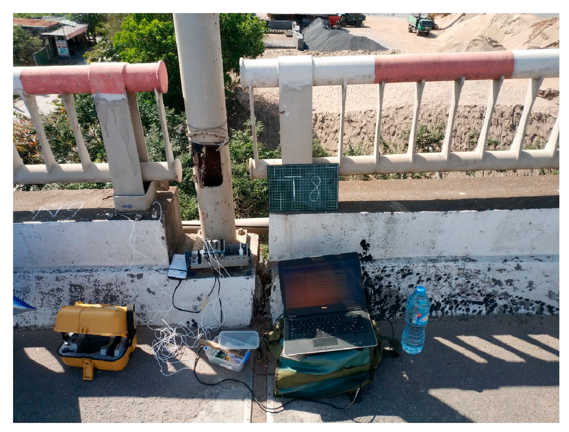
The vibration data collection campaign (acceleration signals) of the main structure of the Lac Quan Bridge was conducted. The campaign aimed to gather a real dataset to evaluate the structural health condition and support research efforts. An actual dataset of 5 vibration sensors was collected from the main bridge. The measuring grid is designed to be deployed to collect vibration data from 5 points on the bridge (
Figure 4). Vibration at points is measured under random stimuli (wind, current, surrounding load, vehicles crossing the bridge, etc.). The equipment used included 5 PCB-353B34 accelerometers. The sensitivity of these sensors ranges from 9.91 to 10.32 mV/m/s
2. The sensors were connected to a CompactDAQ data acquisition system and an NI-9234 data acquisition module. The system was completed with a computer running specialised software for recording and storing the data. The sensors were installed vertically. After arranging and installing measuring devices and sensors, the collection system begins to collect data. The first piece of data will be discarded. After the signal is stable, the data will be recorded and saved. A laptop computer controls the measurement procedure and also collects and stores dynamic responses. The acceleration responses were sampled at a frequency of 1651 Hz. Each measurement interval lasted 30 min.
Figure 5 shows the station set up on the bridge deck for data collection. During the data collection process, the received signals were closely monitored and checked upon completion. The correlation of the signals between the sensors was used for on-site verification. If the data did not meet the requirements, the data collection process would be repeated.
3.2. Single Channel Signal Reconstruction Case
The first case study evaluates the data reconstruction effectiveness of the proposed method in the event of a sensor failure. Single-channel data reconstruction is applied in this scenario. The input to the LSTM network consists of data from the 4 functioning sensors, and the output will be the reconstructed data for the faulty sensor. In this study, acceleration data were simultaneously acquired from five sensor channels during a continuous measurement of around 30 min. The sampling rate was 1651 Hz, resulting in approximately 2.97 million data points per channel. This dataset provides a sufficiently long and dense record to support the training and evaluation of the proposed LSTM-based reconstruction approach.
After pre-processing and restructuring the data as required by the LSTM network, it will be fed into the network for training. The proposed network architecture includes 3 LSTM layers, each comprising 512 memory units. After each LSTM layer, a dropout layer with a rate of 0.25 is added to prevent overfitting. Finally, the data is fed into a densely connected network for training, which outputs the reconstructed data of the faulty sensor. The LSTM model undergoes training using the “Adam” optimisation algorithm, with the loss function being Mean Squared Error (MSE). The dataset will be divided into 2 parts: training and validation. The ratio of these two parts is 80% and 20% respectively. The network is configured to train for a maximum of 1000 epochs, utilising a batch size of 20.
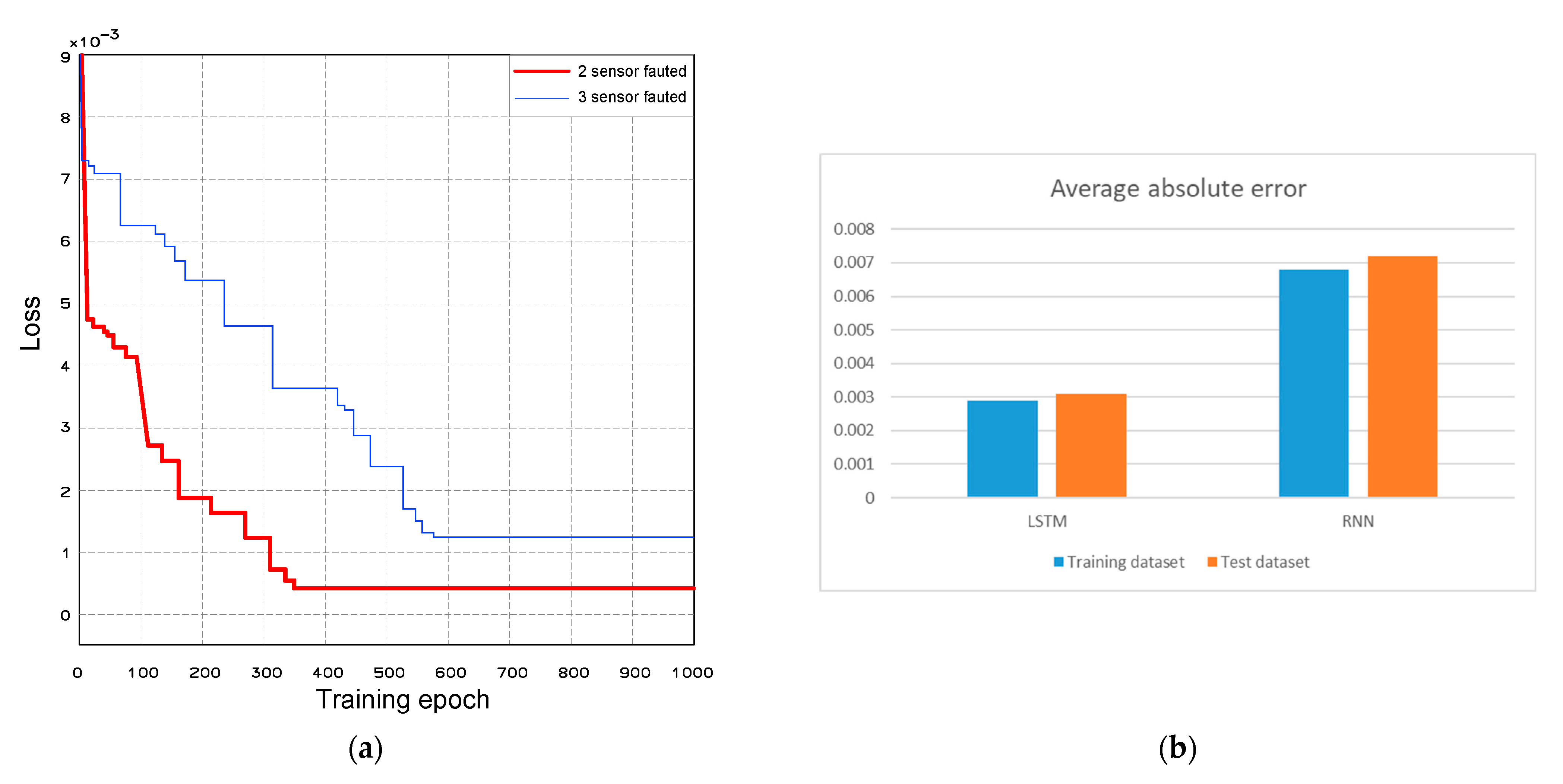
Additionally, in the case of single-channel data reconstruction, to demonstrate the superiority of the LSTM network in solving the problem, the study also uses a simple RNN for data reconstruction. The configuration of the RNN is chosen to be equivalent to the LSTM network, and the training parameters are the same as those used for the LSTM network. The training results of the two methods are shown in
Figure 6.
Figure 6a illustrates the loss during the training process of the LSTM and traditional RNNs. The LSTM outperforms the RNN. The LSTM converges quickly and approaches a value close to 0 within the first 300 epochs, whereas the RNN takes up to 400 epochs. The loss value of the LSTM is closer to 0 compared to the RNN, indicating that the LSTM network has higher accuracy.
Figure 6b shows the mean absolute error of the training and testing sets when using the LSTM and RNN. The error when using the LSTM is very small and close to the actual value, while the RNN yields higher error results. These results demonstrate that the LSTM has a significant advantage over the RNN in terms of time, computational resources, and accuracy.
Figure 7 shows a segment of data reconstructed using LSTM and RNN compared to the actual data. The data reconstructed using LSTM is highly accurate and almost matches the original data. In contrast, the data reconstructed using an RNN is less accurate.
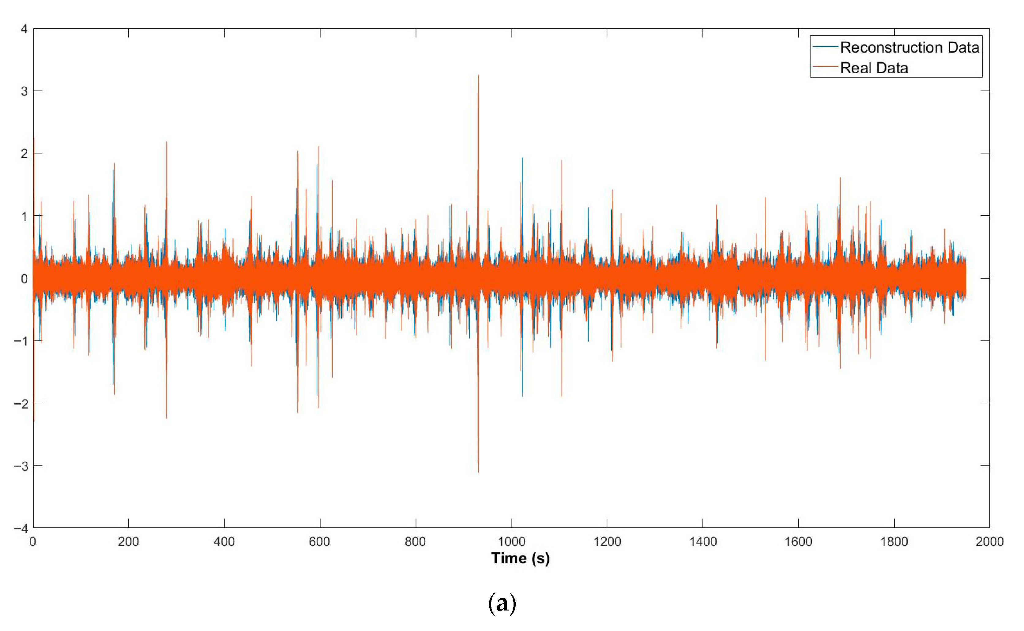
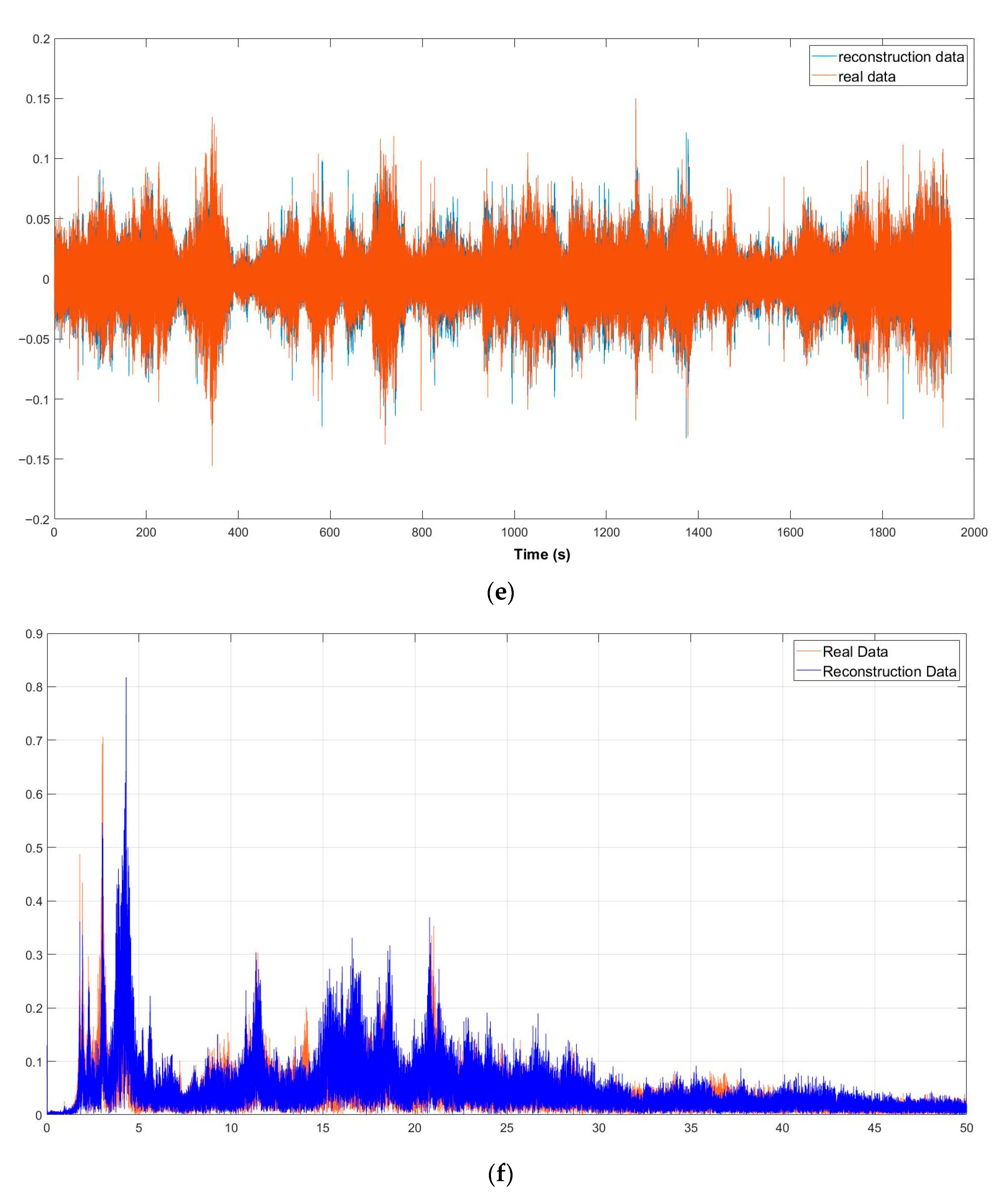
Figure 8 visualises actual and reconstructed data to illustrate the proposed method’s performance better using LSTM. The trained network effectively reconstructed the missing response and vibration information from the sensor fault. A frequency spectrum analysis was also performed on both actual and reconstructed data.
In the single-channel reconstruction scenario, Channel 3 was removed to emulate a faulty sensor. Additional tests with other channels showed similar accuracy (MAE differences < 10%), suggesting that the reconstruction performance does not strongly depend on which channel is missing.
Through the results of the entire dataset reconstructed for one sensor using LSTM, it is evident that the reconstructed data closely matches the actual data. The data points are nearly identical. However, at certain points, the reconstructed data does not completely match the actual data. It is understandable because, in reality, the data will contain many noisy points (sudden spikes caused by vehicle impacts), making complete accuracy impossible. Nonetheless, when analysed in the frequency domain, the reconstructed data aligns well with the frequency spectrum of the actual data.
Figure 8b shows the actual data and the reconstructed data in the frequency domain. Through comparison and analysis, it is evident that the LSTM network yields good results in the case of single-channel data reconstruction. The reconstructed data can effectively represent and replace the actual data.
3.3. Multiple Channel Signal Reconstruction Case
In the case study of single-channel data reconstruction, the results show that the LSTM is capable of reconstructing data with good performance and high accuracy. In the next case study, the LSTM network will be trained to reconstruct data in scenarios where multiple sensors fail (multi-channel data reconstruction). Cases where 2 sensors fail and 3 sensors fail will be examined consecutively.
In the case of multi-channel data reconstruction, the input data for training the LSTM network will be from the functioning sensors, and the output data will be from the failed sensors. The input sensors remain unchanged, while the failed sensors are assigned a value of 0 to simulate failure. The data is pre-processed and then used to train the LSTM network. The configuration and training parameters remain the same as those for single-channel data reconstruction. The dataset contained approximately 2.97 million samples per channel (five channels in total, collected over 30 min at 1651 Hz). When segmented into non-overlapping windows of 200 and 400 samples, this corresponded to about 74,295 and 37,145 sequences, respectively.
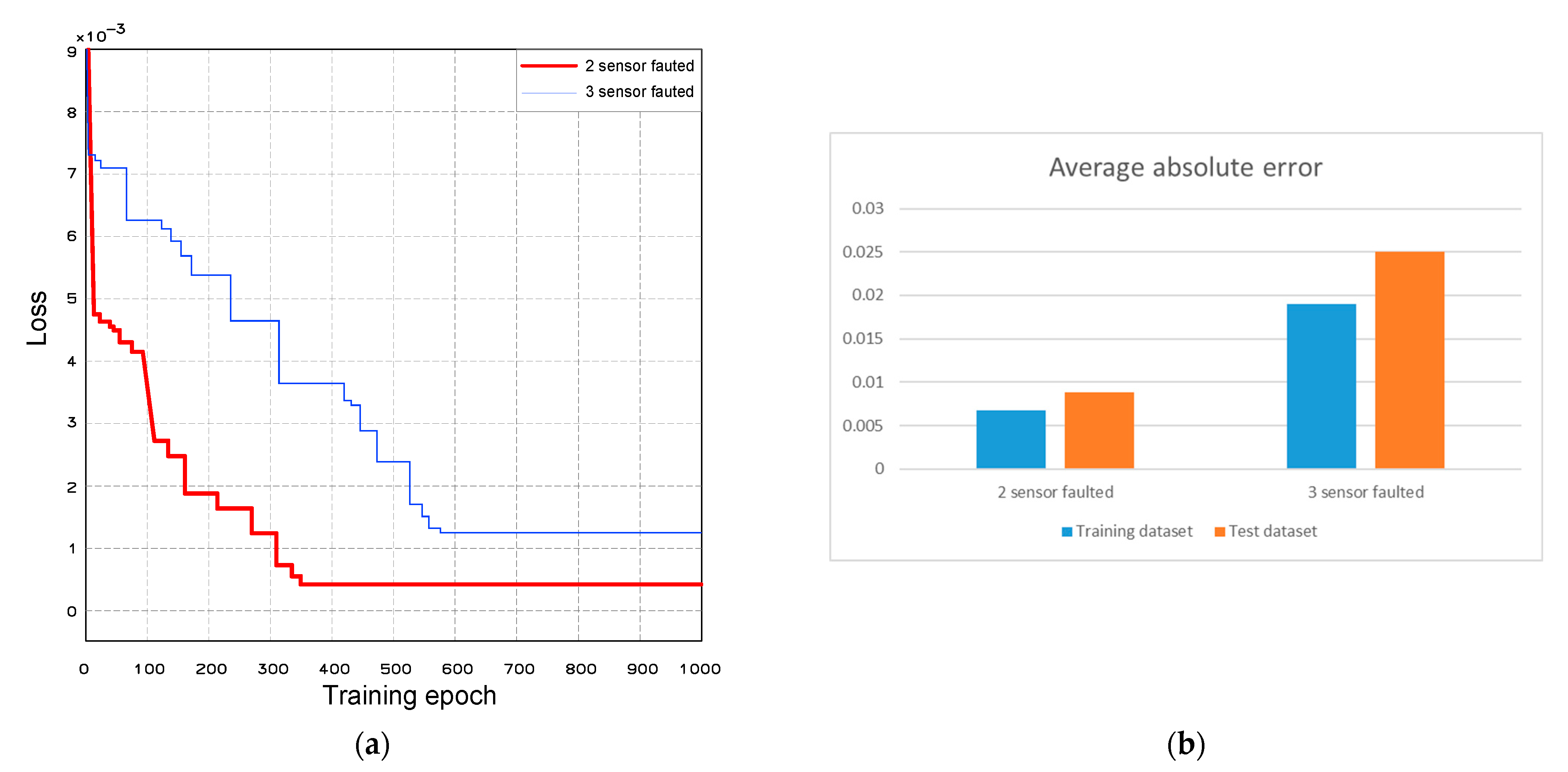
Figure 9 shows the loss during training and the average absolute error.
Figure 9 shows the training results of the network in the cases where 2 and 3 sensors fail and data needs to be reconstructed. In both cases, the loss value of the trained network decreases rapidly in the initial epochs and then gradually converges towards 0. The case with 2 failed sensors demonstrates better performance and results compared to the case with 3 failed sensors. For the loss graph (
Figure 8a), the data reconstruction for 2 sensors converges faster, and the convergence value is closer to 0 compared to the case of 3 failed sensors. Regarding the error value between the actual data and the reconstructed data, the reconstruction of 2 sensors also achieves higher accuracy. It shows that as the amount of data to be reconstructed increases (resulting in increased output) and the amount of input data decreases, the network’s performance and accuracy decrease.
To enhance the network’s performance and accuracy, the study implemented adjustments to the training parameters of the LSTM network. The results show that by tuning the LSTM network parameters for the cases of reconstructing data for 2 sensors and 3 sensors, the accuracy and performance of the method increased significantly. Specifically, the number of LSTM layers was increased from 3 to 4, and the number of memory units per LSTM layer was increased from 512 to 600 units.
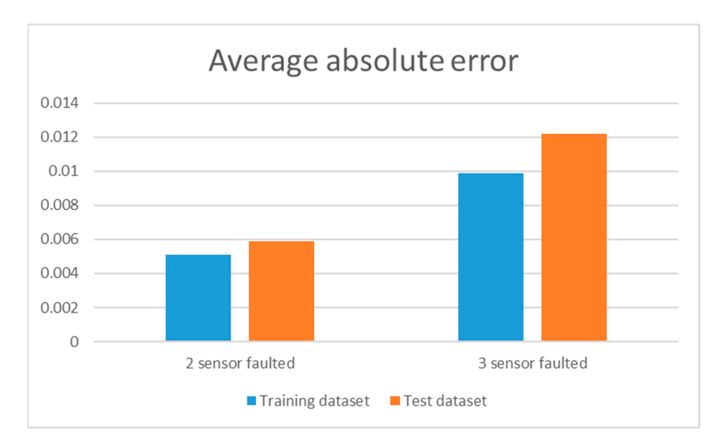
Figure 10 shows the mean error between the reconstructed values and the actual values.
The difference between the actual values and the reconstructed values decreased significantly after adjusting the training parameters. Specifically, for the case of reconstructing data for 2 sensors, the mean error value decreased by 25% for the training set and 33% for the test set. For the case of reconstructing data for 3 sensors, the mean error value decreased by 47% for the training set and 51% for the test set. Thus, the accuracy and performance of the proposed method can be enhanced by utilising suitable network parameters.
Figure 11 shows the reconstructed data in the case of three failed sensors.
The proposed LSTM successfully learned and reconstructed data in cases with multiple channels and data loss. Although the reconstructed data does not precisely match the actual data, it can still be used to monitor structural health. Considering that natural frequencies and vibration modes are the essential fundamental vibration characteristics, the network proposed in this study effectively identified and learned them to capture patterns in vibration data.
To quantify the reconstruction accuracy, MAE, RMSE, NRMSE, and the correlation coefficient between the reconstructed and reference signals are evaluated. In the single-channel case, the LSTM achieved MAE = 0.0029, RMSE = 0.0034, NRMSE = 0.051, and ρ = 0.985. For the more challenging two- and three-channel cases, LSTM obtained MAE = 0.0053 and 0.0190, respectively, with correlation coefficients above 0.92. The error signal analysis confirmed low variance and the absence of systematic bias, suggesting that the reconstructed responses preserve both amplitude and frequency characteristics of the originals.
Experiments were conducted on a workstation with an NVIDIA RTX 3060 (12 GB) GPU and an AMD Ryzen 7 3700X CPU. Two architectures were evaluated: a single-channel LSTM (3 layers, 512 units each; ≈5.25 M trainable parameters) and a multichannel LSTM (4 layers, 600 units each; ≈10.11 M parameters). Under a dataset of ~120,000 windows, the single-channel model was trained in ~55–75 min on GPU (6–8 h on CPU), while the multichannel model was trained in ~95–130 min on GPU (10–14 h on CPU). Average inference latencies were ~0.25–0.35 ms per 200-sample window on GPU (2.5–3.5 ms on CPU) for the single-channel model, and ~0.4–0.6 ms on GPU (4–6 ms on CPU) for the multichannel model. The parameter counts correspond to ~21 MB and ~40 MB memory footprints for the single- and multichannel models, respectively; peak training memory, including activations, remained <1.2 GB on the reported setup.
