Abstract
Accurate prediction of dam deformation is crucial for structural safety monitoring. For enhancing the prediction accuracy of concrete dam deformation and addressing the issues of insufficient precision and poor stability in existing methods when modeling complex nonlinear time series, a concrete dam deformation prediction method based on mode decomposition and Self-Attention-Gated Recurrent Unit (SAGRU) was proposed. First, Variational Mode Decomposition (VMD) was employed to decompose the raw deformation data into several Intrinsic Mode Functions (IMFs). These IMFs were then classified by K-means algorithm into regular signals strongly correlated with water level, temperature, and aging factors and weakly correlated random signals. For the random signals, an Improved Wavelet Threshold Denoising (IWTD) method was specifically applied for noise suppression. Based on this, a Deep Learning (DL) model based on SAGRU was constructed to train and predict the decomposed regular signals and the denoised random signals, respectively. And finally, the sum of the calculation results of each signal can be output as the predicted deformation. Experimental results demonstrate that the proposed method outperforms existing models in both prediction accuracy and stability. Compared to LSTM, this method reduces the Mean Absolute Error (MAE) and Root Mean Square Error (RMSE) by approximately 30.9% and 27.2%, respectively. This provides an effective tool for analyzing concrete dam deformation and offers valuable reference directions for future time series prediction research.
1. Introduction
Concrete dams are the core facilities of water conservancy projects, which play a crucial role in flood control, disaster mitigation, water resource regulation, clean energy production, and economic benefits. During a concrete dam’s long service life, it is subject to complex environmental conditions and cyclic loads, causing gradual accumulation of deformation in the dam body and threatening structural safety. To assess dam safety instantly, the dam health monitoring system compares deformation monitoring data with mathematical model prediction results to determine whether the structural behavior is still within the dam’s safety threshold [1]. Therefore, a high-precision deformation prediction method is important to concrete dams.
The accurate prediction of dam deformation hinges on a profound understanding of its underlying physical drivers. The deformation behavior is a macroscopic manifestation of complex interactions among multiple factors, which are traditionally decomposed into three primary components [2]: the hydrostatic component, caused by reservoir water pressure and its effect on the foundation; the temperature component, resulting from concrete’s thermal expansion and contraction; and the time-dependent component, encompassing irreversible effects like concrete creep, aging, and foundation consolidation. This physical decomposition forms the foundational paradigm for understanding and predicting dam behavior. Traditional prediction models are deeply rooted in this physical understanding. Statistical models, such as the Hydrostatic-Season-Time (HST) model, leverage this decomposition for prediction based on linear assumptions [3]. While robust and interpretable, their inherent linearity can limit their ability to capture complex nonlinear behaviors. Conversely, physics-based numerical models, such as the Finite Element Method (FEM), offer a more rigorous representation by incorporating detailed material properties (e.g., elastic modulus, creep laws, thermal expansion coefficient) and geological conditions (e.g., foundation permeability, rock mass integrity) [4,5,6]. However, the application of high-fidelity FEM models is often constrained by the limited availability and uncertainty of the required input parameters, making them computationally expensive and difficult to calibrate for routine forecasting.
In this context, the operational data routinely collected by dam safety monitoring systems provides a valuable pathway for deformation analysis, spurring the adoption of data-driven machine learning (ML) techniques. These models can learn complex, nonlinear mappings directly from historical data. A critical step in this data-driven pipeline is signal preprocessing to extract meaningful information from raw monitoring sequences.
This process mainly includes decomposition and denoising. For decomposing deformation sequences, different algorithms have their own advantages and disadvantages. For example, the wavelet analysis [7] provides thorough signal decomposition but suffers from poor adaptability and subjective scale selection. Empirical Mode Decomposition (EMD) [8] offers adaptive advantages and high time-frequency resolution yet remains vulnerable to mode aliasing. Although the improved method Ensemble Empirical Mode Decomposition (EEMD) [9] can suppress modal aliasing, it still has the drawbacks of random decomposition layers and high computational complexity. Compared to the above methods, Variational Mode Decomposition (VMD) [10] demonstrates superior robustness, which can simultaneously solve the modal aliasing of EMD and avoid the uncontrollable number of EEMD layers. Regarding denoising after decomposition, in traditional Wavelet Threshold Denoising (WTD), the hard threshold method can easily cause signal oscillation, while the soft threshold method may cause constant deviation [11]. To solve the above problems, B. Xie et al. [12] proposed an Improved Wavelet Threshold Denoising (IWTD) method. By refining the threshold calculation rules and threshold function, it dynamically adjusts the denoising intensity based on local signal characteristics, effectively suppressing noise while better preserving useful signals. This method is particularly suitable for processing highly volatile, complex noise non-stationary sequences; hence, it was selected in this study to achieve more precise denoising results.
As for deformation prediction models, statistical models based on regression are initially widely used [13]. Basic regression models include Multiple Linear Regression (MLR) [14], Stepwise Regression (SR) [15], partial least squares regression [16], and so on. While the statistical model used frequently is the Hydrostatic-Season-Time (HST) model. based on MLR. Although the above model has been widely used in deformation prediction, linear regression is essentially not suitable for establishing high-dimensional relationships, which limits the prediction accuracy and robustness of statistical models [17]. Afterwards, with the development of computer technology, Machine Learning (ML) [18] algorithms capable of handling nonlinear problems have been widely applied to deformation prediction. ML includes Artificial Neural Networks (ANN) [19], Support Vector Machines (SVM) [20], Multilayer Perceptron (MLP) [21], Extreme Learning Machines (ELM) [22], Random Forests (RF) [23], and so on. Compared to traditional statistical models, ML typically demonstrates better predictive performance and accuracy. However, ML always treats dam deformation prediction as a static regression problem, while deformation is a real-time dynamic process. To capture the time dependency of deformation data, Deep Learning (DL) [24] algorithms have been introduced. For instance, the Recurrent Neural Network (RNN) [25] model, which transmits historical information through hidden states, can effectively handle short-term sequences problems but may encounter gradient disappearance in long-term sequences predictions. To address this issue, Long Short-Term Memory (LSTM) networks [26] introduced a forgetting mechanism to ensure performance in predicting long sequences, which has been widely applied to dam deformation prediction [27,28,29,30]. However, it should also be noted that LSTMs have a large number of parameters, relatively slow training processes, and are prone to overfitting under small sample sizes or noisy interference. To alleviate overfitting, Gated Recurrent Unit (GRU) [31,32] introduces a gating mechanism to dynamically control the retention and forgetting of information, balancing computational accuracy and efficiency. Nevertheless, it should be noted that the sensitivity of GRU primarily lies in capturing temporal features such as trends and periodicity, while potentially losing some interactions between other influence factors like water level and temperature with deformation. Therefore, to further enhance GRU’s feature extraction capability, Tang Yan et al. [33] added the self-attention mechanism [34,35,36,37] into GRU, enabling adaptive selection of more important information from all input features, thereby optimizing network performance and demonstrating improved predictive performance in deformation prediction.
However, a significant gap persists between pure data-driven applications and the fundamental principles of dam engineering. This disconnect is evident in two interconnected dimensions where prevailing methodologies often overlook the physical context:
First, in the domain of signal preprocessing, existing approaches apply decomposition and denoising as largely blind mathematical tools. The core limitation is the absence of a quantitative framework to establish correlations between decomposed components (e.g., IMFs) and their physical origins (water pressure, temperature). This leads to coarse-grained denoising strategies that risk distorting signal features carrying critical physical meaning, while simultaneously failing to adequately suppress noise unrelated to structural behavior. The consequence is a loss of mechanistic fidelity in the input data before it even reaches the prediction model.
Second, in the modeling domain, while algorithms like GRU capably capture temporal dependencies, they often inadequately represent the underlying physics. Most models fail to simultaneously account for the full dynamic temporal evolution of deformation and the complex, nonlinear interactions between the multiple physical driving factors. This narrow focus limits their generalizability and results in poor robustness—manifesting as susceptibility to overfitting and performance degradation under high-noise or small-sample scenarios, which are common in real-world monitoring. Furthermore, the “black-box” nature of these models provides limited interpretability into the causal relationships governing the predictions, thus offering little engineering insight beyond point forecasts.
First, we develop a physics-informed preprocessing framework that synergistically combines Variational Mode Decomposition (VMD), K-means clustering, and Improved Wavelet Threshold Denoising (IWTD). Its innovation lies in quantitatively classifying the decomposed intrinsic mode functions (IMFs) into “regular signals” strongly correlated with physical drivers (e.g., hydrostatic pressure, temperature effects) and “random signals” weakly correlated with them. This enables a directed denoising strategy, where IWTD is applied precisely to “random signals” while rigorously preserving “regular signals” that carry critical physical meaning, thereby enhancing the mechanistic fidelity of the input data. Second, to simultaneously capture temporal dynamics and the nonlinear interactions among physical drivers, a Self-Attention Gated Recurrent Unit (SAGRU) model is introduced as the predictor. This model leverages the GRU’s strength in modeling temporal dependencies while employing a self-attention mechanism to adaptively weight the importance of all input features, thereby explicitly modeling complex nonlinear interactions. The measurable outcome is a significant improvement in prediction accuracy, such as a 33.3% reduction in Root Mean Square Error (RMSE), compared to benchmarks like standard GRU and LSTM. This design also provides a step towards improved model interpretability by revealing the dynamic influence of different factors.
The proposed end-to-end workflow, which systematically integrates “decomposition–clustering–denoising” preprocessing workflow with the SAGRU prediction model, is comprehensively validated through a case study. The results demonstrate its enhanced performance not only in quantitative accuracy but also in robustness against noise and reliability in tracking deformation trends.
The paper is organized as follows: After the introduction, Section 2 presents preprocessing methods for deformation data including VMD, K-means clustering and IWTD. Then, Section 3 introduces the deformation prediction model, namely, SAGRU combined with GRU and self-attention mechanism. After that, Section 4 presents the workflow of the dam deformation prediction method proposed in this paper. Subsequently, Section 5 applies this prediction method to a certain arch dam to show the pre-processing effect and the deformation prediction effect. Finally, Section 6 presents the conclusions.
2. Data Preprocessing Methods
The data preprocessing framework used in this paper includes mode decomposition and denoising, which are realized by Variational Mode Decomposition (VMD) and Improved Wavelet Threshold Denoising (IWTD), respectively. Notably, feature extraction and K-means clustering are performed on the decomposed signals to ensure that only random signals are accurately denoised. These works can preserve the regular features of data as much as possible during preprocessing. Subsequently, the basic principles of the methods above are presented as follows.
2.1. Variational Mode Decomposition
Variational Mode Decomposition (VMD) is a completely non-recursive adaptive signal decomposition method, which can decompose complex signals into sparse Intrinsic Mode Functions (IMFs). The decomposition process is essentially solving a constrained variational problem presented by Equation (1).
More computational details can be found in Reference [11]. Notably, parameters to be entered in VMD include and the penalty parameter . And is used to control the bandwidth during iteration, that is to force the energy of to concentrate around the central frequency .
This study employs the Gray Wolf Optimization Algorithm (GWO) to optimize the aforementioned two key parameters in VMD. Detailed optimization procedures of the Gray Wolf Algorithm are documented in Reference [38]. When optimizing VMD parameters using GWO, it is necessary to construct a fitness function to measure the optimization performance, and permutation entropy [39] was selected as the function in this study. Permutation entropy is an entropy measure of time series complexity. Compared to other time series complexity parameters (such as Lyapunov exponents, fractal dimension, and approximate entropy), it is simpler to compute and exhibits stronger resistance to interference. Furthermore, this method enables precise and efficient localization of signal breakpoints while quantitatively assessing random noise within signal sequences, making it particularly suitable for signals containing dynamic and observational noise [40]. Its principle is as follows:
- (1)
- The time series is discrete with a length of , and the following matrix is obtained via spatial reconstruction of the sequence,
- (2)
- The components rearranged in ascending order to obtain the positions of each element within the vector to form a group of symbol sequences . The m-dimensional space maps different symbolic sequences with a total of species.
- (3)
- The number of each r symbol sequence divided by m! is calculated, and the total number of occurrences of different symbolic sequences is calculated as the probability of occurrence of different symbolic sequences . Furthermore, permutation entropy of the time series is calculated as
- (4)
- The maximum value of permutation entropy is , and per mutation entropy is normalized as follows:
The magnitude of permutation entropy and the amplitude of signal noise are related: when the value is smaller, the sequence is simpler and more regular; in contrast, when the value is larger, the sequence is more complex and random.
2.2. K-Means Clustering
The K-means clustering algorithm [41] can divide data into several non-overlapping clusters and minimize the intra-cluster sum of squares errors as shown in Equation (2).
The detailed iterative calculation process is described in Reference [42]. In this paper, K-means clustering is used to classify the Intrinsic Mode Functions (IMFs) obtained by Variational Mode Decomposition (VMD) into two clusters: regular signals and random signals. The classification criteria used are the Pearson correlation coefficients between deformation and deformation influencing factors. The factors include the water depth in front of the dam, dam body temperature, and time-dependent effect raised by the Hydrostatic-Season-Time (HST) model, whose expressions are given in Equation (6), Equation (7) and Equation (8), respectively.
2.3. Improved Wavelet Threshold Denoising
The Wavelet Threshold Denoising (WTD) establishes a mathematical relationship between the original signal and the wavelet coefficients based on wavelet transformation. During the transition, threshold function quantization is performed with the wavelet coefficients to achieve denoising [43]. To overcome the shortcomings of traditional threshold functions, the Improved Wavelet Threshold Denoising (IWTD) [12] adopts a new threshold function calculation method presented in Equation (9).
In Equation (9), calculated by Equation (10) is the wavelet coefficient from wavelet transform, calculated by Equation (11) is the wavelet threshold. In Equation (10), is the observed signal, represents the mother wavelet, is the signal length. As for Equation (11), is the number of decomposition layers for wavelet transform, is the standard deviation in the noise.
3. Self-Attention-Gated Recurrent Unit
The Self-Attention-Gated Recurrent Unit (SAGRU) is capable of fully capturing the important information within sequences. SAGRU retains the temporal modeling capabilities of GRU which uses the ‘update gate’ and the ‘reset gate’ to control the retention and forgetting of historical information, respectively. Specifically, the output of current moment can be obtained through the calculations of the above two gates based on the input vector of the current moment and the hidden state of the previous moment. Here, to better catch key features, a self-attention mechanism is added, which primarily relies on internal data information for attention interaction to improve the performance of prediction model [34]. The internal structure of the GRU is shown in Figure 1.
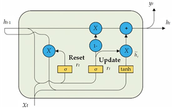
Figure 1.
Internal structure of a GRU.
The detailed computational process is presented in Reference [33]. Additionally, comprehensively considering the learning performance and consumption of the model, two GRU layers with dropout layers are employed in this paper to mitigate overfitting, while the self-attention mechanism is added between the two GRU layers to enhance the model’s predictive performance. Finally, a fully connected layer is used to process and output the predicted values.
In this paper, SAGRU is used to train and predict the denoised random signals and the decomposed regular signals separately. And the sum of the predicted results of all signals will be output as the predicted deformation. It is worth noting that in the prediction for random signals, only the denoised random signals themselves need to be input. That is because SAGRU can learn long-term dependencies fully to ensure the accuracy of prediction. While in the prediction for regular signals, the input includes not only the regular signals themselves but also the deformation influence factors presented in Section 2.2, which enables SAGRU to further capture the interactive information of all input features and fully ensure prediction performance.
After constructing the SAGRU model, Bayesian optimization (BO) was employed to optimize parameters such as the initial learning rate, window size, dropout rate and number of GRUs. This process yielded the optimal hyperparameters.
4. Concrete Dam Deformation Prediction Method
The workflow of the concrete dam deformation prediction method based on mode decomposition and the Self-Attention-Gated Recurrent Unit (SAGRU) can be divided into four parts as shown in Figure 2.
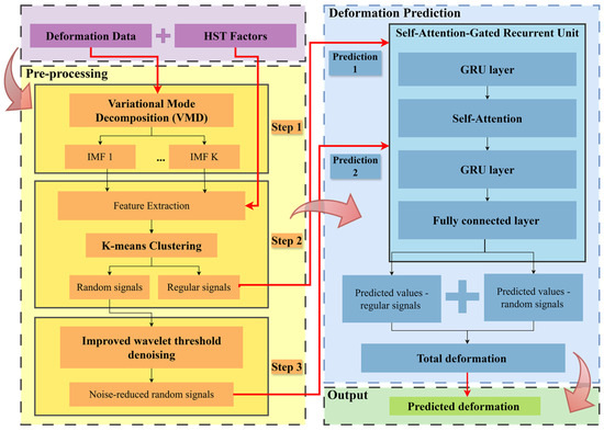
Figure 2.
Workflow of the concrete dam deformation prediction method based on mode decomposition and SAGRU. The workflow is divided into Input in purple, Pre-processing in yellow, Deformation Prediction in blue and Output in green separated by gray dashed boxes. Notably, Pre-processing is divided into three steps separated by gray solid-line boxes. Deformation Prediction includes twice predictions for regular signals and random signals separately. In addition, red thick lines and arrows indicate the output-input relationship between different modules, while black thin lines and arrows within each module indicate ordinary process relationships.
- Part 1: Input. The input information mainly includes deformation monitoring data and deformation influencing factors raised by the Hydrostatic-Season-Time (HST) model (water depth in front of the dam, dam body temperature, and time-dependent effect calculated by Equation (3), Equation (4) and Equation (5), respectively).
- Part 2: Pre-processing. The pre-processing can be divided into three steps as follows.
- Step 1: Variational Mode Decomposition (VMD) is used to decompose deformation monitoring data into ‘K’ Intrinsic Mode Functions (IMFs). Notably, the parameters K and penalty parameter α need to be set manually. Considering the degree and effectiveness of decomposition for general deformation data, K is typically set to 3~10, and α is commonly set to 2000~10,000, with higher values chosen for more complex signals.
- Step 2: Extract the features of each IMF, namely the Pearson correlation coefficients between IMF and the HST factors. Then, K-means clustering is used to divide the regular signals and random signals into two clusters. Next, the regular signals can be output into SAGRU to perform Prediction 1. It is worth noting that Prediction 1 also requires the simultaneous input of HST factors.
- Step 3: Improved Wavelet Threshold Denoising (IWTD) is used to denoise random signals, and then the denoised signals can be output into SAGRU to perform Prediction 2.
- 3.
- Part 3: Deformation Prediction. This process is mainly performed by SAGRU including Prediction 1 and Prediction 2, which output prediction values based on regular signals and random signals, respectively. Here, the hyperparameters that need to be set include the model learning rate, sliding window length, batch size and the number of GRU nodes. And the genetic algorithm [44] is used to optimize the parameters to ensure the representational capability of model. Additionally, the total deformation output is the sum of the predicted results of all signals.
- 4.
- Part 4: Output. The final predicted deformation is the total deformation output by Part 3.
5. Empirical Verification
To present the validity of the proposed concrete dam deformation prediction method, the deformation monitoring data of a specific concrete double-curved arch dam was used to carry out empirical verification. The dam has a crest elevation of 1885.0 m, a maximum dam height of 305 m, and consists of 26 dam sections. The three-dimensional model of the dam [45] is shown in Figure 3.
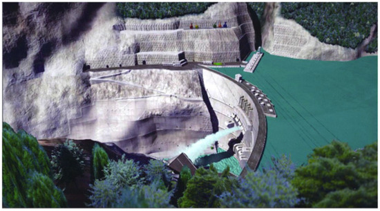
Figure 3.
Example of a Three-Dimensional Model of a Hyperbolic Arch Dam.
The predictive performance of the model was validated using observation data from the PL16-3 vertical line measurement point at an elevation of 1778.25 m and the PL16-4 vertical line measurement point at an elevation of 1730.25 m, collected between 8 December 2013, and 18 June 2017. The measured process lines of the point displacement and the upstream reservoir water level changes are presented in Figure 4. Here, the data was divided into a training set and a test set in the ratio of 7:3.
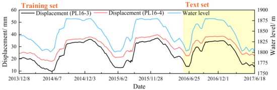
Figure 4.
Monitoring displacement and water level process lines. The horizontal axis represents data. The lines in black and red present the displacement corresponding to the left vertical axis and the line in blue is the water level matching with the right vertical axis. In addition, the white area covers the training set, and the yellow area covers the test set.
5.1. Pre-Processing Effect
The raw deformation data was decomposed into five intrinsic modal functions (IMFs) via Variational Modal Decomposition (VMD), with penalty parameters of 2212 (PL16-3) and 2317 (PL16-4). These hyperparameters were optimized using the GWO algorithm described in Section 2.1. And then these IMFs were divided into two clusters with K-means clustering as presented in Figure 5. Next, the Improved Wavelet Threshold Denoising (IWTD) was used for the random signals, where the wavelet basis function was selected as sym7 and the decomposition layer was 4. Furthermore, to verify the denoised effect of IWTD, the Wavelet Threshold Denoising (WTD) with soft thresholds was used simultaneously to process the random signals. And the comparison of the denoised results is shown in Figure 6.


Figure 5.
IMFs decomposed by VMD after clustering (unit: mm). The horizontal axes of all subplots represent the time in days. The blue lines in the blue dashed box above represent the regular signals. The red lines in the red dashed box below represent the random signals.
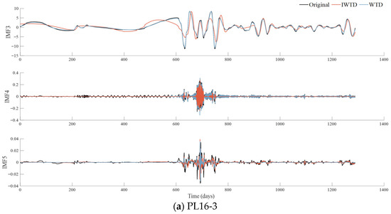
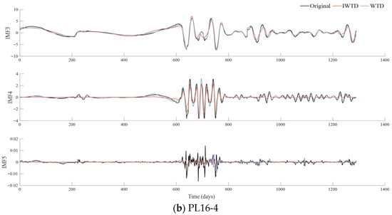
Figure 6.
Random signals before and after denoising separately using IWTD and WTD (unit: mm). The horizontal axes of all subplots represent the time in days. The black line in each subplot represents the original IMF, the red line represents the results after IWTD processing, and the blue line represents the results after WTD processing.
As shown in the denoised signal waveform in Figure 4, the signal processed by IWTD demonstrates significant advantages in its time-domain characteristics. Particularly in IMF3, the IWTD method effectively suppresses high-frequency oscillations while retaining the main peak features, whereas the noise reduction performance of conventional WTD is notably insufficient.
For example, in the IMF3 component, for measurement points 16-3 and 16-4 with large original amplitudes, the noise extremum ranges extracted by the IWTD method are [−7.1298, 6.7035] and [−2.0844, 1.9974], respectively. In comparison, the traditional WTD method yielded noise extremum ranges of [−0.7129, 0.6408] and [−0.8441, 0.6668] at the same locations. In terms of extreme value span, the noise amplitude identified by IWTD is significantly larger than that of WTD, indicating that IWTD can more effectively capture stronger noise components hidden in the signal, reflecting its superior noise extraction capability.
For the relatively smaller IMF4 and IMF5 components, the noise extremes extracted by IWTD at the corresponding measurement points were [−0.0924, 0.0774], [−1.8386, 1.6293] (IMF4) and [−0.0272, 0.0206], [−0.0149, 0.0142] (IMF5). The noise extremes obtained by the WTD method were [−0.0874, 0.0637] and [−0.8993, 0.857] (IMF4), and [−0.0162, 0.0135] and [−0.0125, 0.0090] (IMF5). Comparisons reveal that IWTD consistently covers wider extremum intervals than WTD across both high-amplitude and low-amplitude noise components, indicating more consistent sensitivity and broader applicability in identifying noise of varying intensities. Particularly for faint noise like IMF5, IWTD maintains relatively high extraction amplitudes, further highlighting its superior noise detection capability over traditional methods under low signal-to-noise ratio conditions.
In summary, IWTD can effectively extract and suppress noise components at various scales while ensuring the integrity of main signal features. Specifically for processing non-stationary signals containing large-amplitude noise, IWTD demonstrates significant technical advantages. Notably, since the preprocessing only performs identification and removal of noise for random signals while leaving regular signals untreated, the retention and presentation of the samples trend characteristics can be maximized for enhancing the ability to characterize the deformation behavior of dam.
5.2. Deformation Prediction Effect
After denoising the measured dam deformation data, the top 70% of the data were selected to train the displacement prediction model, while the remaining 30% served as the test set to evaluate model performance. The model employed a genetic algorithm for parameter selection. The optimization intervals and optimal parameters for monitoring points PL16-3 and PL16-4 are shown in Table 1 and Table 2, respectively.

Table 1.
Range and results of BO parameter optimization of PL16-3.
Table 2.
Range and results of BO parameter optimization of PL16-4.
The Self-Attention Gated Recurrent Unit (SAGRU) was employed to train and predict both conventional signals and denoised random signals, with a maximum iteration limit of 50 iterations. The final deformation was obtained by summing the predicted values of all signals. To validate SAGRU’s prediction accuracy, both the Gated Recurrent Unit (GRU) and Long Short-Term Memory (LSTM) networks were applied to analyze the same data, with results shown in Figure 7 and Figure 8.
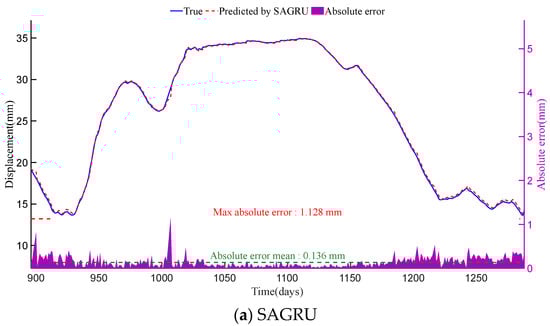
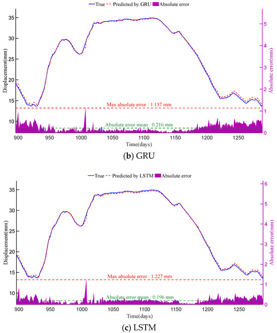
Figure 7.
Displacement prediction results and absolute errors of SAGRU, GRU and LSTM at PL16-3 monitoring point. The horizontal axes of all subplots represent the time in days. The blue line and red dashed line in each subplot (corresponding to the left vertical axis) represent the true displacement (i.e., original monitoring data) and the predicted results of each method, respectively. Meanwhile, the purple shaded area in each subplot (corresponding to the right vertical axis) indicates the distribution of absolute errors.
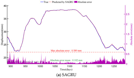
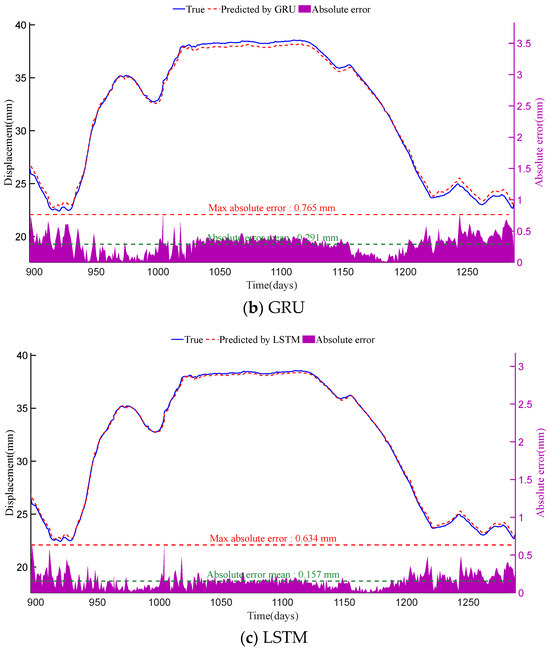
Figure 8.
Displacement prediction results and absolute errors of SAGRU, GRU and LSTM at PL16-4 monitoring point. The horizontal axes of all subplots represent the time in days. The blue line and red dashed line in each subplot (corresponding to the left vertical axis) represent the true displacement (i.e., original monitoring data) and the predicted results of each method, respectively. Meanwhile, the purple shaded area in each subplot (corresponding to the right vertical axis) indicates the distribution of absolute errors.
As shown in Figure 7 and Figure 8, among the three methods, SAGRU’s predictions align most closely with actual values. Its absolute error distribution is concentrated with minimal fluctuation, demonstrating exceptional stability and predictive accuracy. In contrast, although LSTM and GRU both belong to deep learning (DL) methods, their prediction results still fall slightly short of SAGRU. This finding indicates that standard recurrent neural networks still have room for optimization when capturing complex dependencies.
To validate the effectiveness and accuracy of the SAGRU algorithm, LSTM and GRU models commonly used for dam deformation prediction were applied to analyze the same dataset. Figure 9 shows the residual histograms.
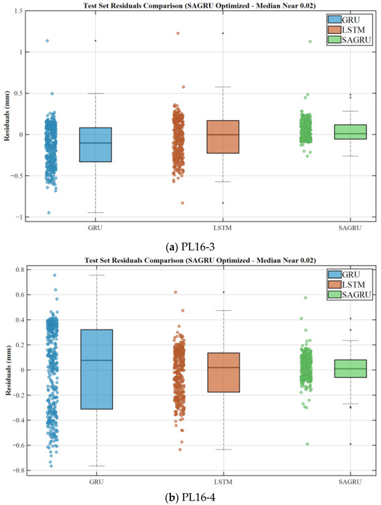
Figure 9.
Residual histograms for GRU, LSTM and SAGRU models.
Additionally, regarding the computational cost of SAGRU compared to GRU and LSTM, as shown in Table 3.
Table 3.
Computational cost of SAGRU, GRU and LSTM (unit: s).
As shown in Table 3, the computational cost of the SAGRU model at monitoring points PL16-3 and PL16-4 falls between that of GRU and LSTM, closely approaching GRU and thus acceptable.
To further compare the predictive performance of each method, quantitative comparisons were conducted using Mean Square Error (MSE), Mean Absolute Error (MAE) and Root Mean Square Error (RMSE). And the metrics for each model are summarized in Table 4.
Table 4.
Model evaluation metrics.
As shown in Table 4 of the performance comparison, the SAGRU model demonstrates outstanding predictive capability at both monitoring points PL16-3 and PL16-4. Specifically, SAGRU achieved the lowest values across all three-evaluation metrics—Mean Squared Error (MSE), Mean Absolute Error (MAE), and Root Mean Squared Error (RMSE)—indicating superior accuracy and stability.
Compared to the GRU model, SAGRU’s advantages are particularly pronounced. For instance, at monitoring point PL16-4, SAGRU’s mean squared error is only 17.0% of GRU’s, while its mean absolute error is approximately 69.0% lower. This substantial performance gap highlights the critical role of SAGRU’s built-in self-attention mechanism in capturing complex temporal dependencies. Although the LSTM model outperformed the GRU, it still lagged behind SAGRU. At node PL16-3, LSTM’s MAE was 44.4% higher than SAGRU’s, underscoring SAGRU’s optimization advantages over traditional recurrent architectures.
Regarding the GRU model, its performance exhibited the greatest instability among all tested deep learning methods. While comparable to LSTM at the PL16-3 node, metrics deteriorated sharply at the PL16-4 node, suggesting potential limitations in generalizing across distinct feature data within the same dataset.
Overall, the tabular data confirms the critical importance of architectural innovation. By effectively integrating gated recurrent units with self-attention mechanisms, SAGRU establishes a leading position in this time series forecasting task, with statistically superior results compared to standard LSTM and GRU models. The findings strongly validate that the proposed SAGRU architecture provides a more robust and reliable solution for sequence modeling.
6. Discussion
Although the prediction model based on VMD-IWTD and SAGRU proposed in this study demonstrated satisfactory performance in case applications, several inherent limitations remain to be addressed in future work.
First, the robustness of the model under extreme environmental conditions requires further validation. The data employed in this study primarily reflect historical normal operating conditions. However, during rare events such as extreme floods, exceptionally low temperatures, or strong earthquakes, the deformation mechanisms of dams may undergo nonlinear abrupt changes, exceeding the patterns learned by the current model from historical data. Under such circumstances, the predictive accuracy of the model may significantly decline. Future work should involve testing the model against monitoring data from such extreme events or, alternatively, employing high-fidelity finite element models to generate physically consistent synthetic data for augmenting the training set, thereby enhancing the model’s robustness.
Second, the method heavily relies on the integrity and quality of input data. The preprocessing and prediction workflow proposed in this paper assumes access to continuous, high-frequency monitoring data. However, in real-world engineering scenarios, sensor failures or communication interruptions may cause prolonged data gaps or abnormal outliers. This study does not explore countermeasures for such data-missing scenarios, such as repairing data chains through interpolation, generative models, or transfer learning to maintain stable prediction system operation. This represents an important future research direction.
Third, the model’s interpretability remains an area for improvement. Although the self-attention mechanism provides feature importance weights to some extent, the entire “decomposition-denoising-prediction” pipeline remains a complex “black-box” model as a whole. Deepening the integration between data-driven models and physical mechanisms—such as incorporating mechanical equations as constraints during training—is crucial for generating predictions that are not only accurate but also physically interpretable. This is essential for gaining domain experts’ trust and advancing practical applications in safety decision-making.
Finally, the scope of influencing factors considered is inherently constrained by the available data and the choice of the base model. This study employed the HST model for factor identification, focusing on water level, temperature, and time. Consequently, more detailed material and geological parameters—such as concrete porosity, permeability, and foundation stability—which are integral to physics-based models like the HTT model and corresponding finite element analyses, were not incorporated. The primary data source for this work was historical monitoring data from an actual dam, which did not include these specific parameters. Future research should prioritize the collection of such data and explore the development of hybrid models that can assimilate both high-frequency monitoring data and intermittent physical property measurements, thereby achieving a more comprehensive representation of the dam’s structural state.
Acknowledging these limitations does not diminish the contributions of this research. Rather, it serves to clearly delineate its application boundaries and chart a coherent path for future research aimed at creating more robust, generalizable, and physically grounded predictive models for dam safety.
7. Conclusions
This paper proposes a deformation prediction method for concrete dams based on modal decomposition and self-attention gated recurrent units (SAGRU). Through comparative analysis with other typical spatio-temporal models, the accuracy and applicability of the proposed model are validated. The conclusions of this paper can be summarized as follows:
- (1)
- To preprocess the actual deformation monitoring data, Variational Mode Decomposition (VMD) was integrated with an Improved Wavelet Threshold Denoising (IWTD) technique. This combined approach utilizes K-means clustering to identify and eliminate stochastic noise, while preserving representative signal components to retain the inherent trends of the original data. This strategy enables targeted denoising that preserves deformation characteristics strongly correlated with hydrostatic and thermal drivers, thereby enhancing the physical fidelity of the input data for subsequent prediction.
- (2)
- For deformation prediction, a Self-Attention Gated Recurrent Unit (SAGRU) model was proposed. The architecture leverages the nonlinear dynamic modeling strength of Gated Recurrent Units (GRUs), augmented by a self-attention mechanism that adaptively prioritizes salient temporal features and captures long-range dependencies. This leads to a systematic improvement in prediction accuracy and temporal coherence.
- (3)
- Empirical evaluations confirm that the SAGRU model achieves superior performance over conventional models such as GRU and LSTM. Compared to LSTM, this method reduces the Mean Absolute Error (MAE) and Root Mean Square Error (RMSE) by approximately 30.9% and 27.2%, respectively. The incorporation of self-attention effectively alleviates the information decay typical in standard GRU networks when handling long sequences, yielding a 33.3% reduction in Root Mean Square Error (RMSE) and a 39.8% reduction in Mean Absolute Error (MAE). These results not only highlight the efficacy of the structural enhancements but also demonstrate the value of combining deep structures with attention mechanisms, advancing beyond the nonlinear expressive power of traditional statistical models (e.g., MLR) and shallow machine learning (e.g., SVM), as well as the limited long-range context modeling of standard LSTM/GRU networks.
- (4)
- This study simultaneously clarifies the theoretical boundaries and application prerequisites of the proposed data-driven methodology. It is important to note that the SAGRU model, owing to its inherent self-attention mechanism, inevitably incurs higher computational overhead than traditional GRU models. Furthermore, its performance exhibits sensitivity to hyperparameter configuration, necessitating systematic tuning to achieve optimal outcomes.
- (5)
- Empirical validation is based on a specific arch dam dataset. The model’s generalizability across different dam types (e.g., gravity dams, buttress dams) and significantly divergent environmental conditions remains insufficiently verified, necessitating further investigation into its cross-scenario generalization capabilities. More fundamentally, the model’s current formulation, while accurate under normal operating conditions, does not explicitly incorporate intrinsic material and geotechnical properties such as concrete porosity, soil stability, and foundation permeability. The absence of these parameters highlights a critical direction for future work: the development of truly hybrid models that can assimilate both high-frequency monitoring data and fundamental physical properties to enhance long-term reliability and generalizability.
Looking forward, this study clearly demonstrates that enhancing computational accuracy serves as a crucial means to achieve engineering safety objectives, rather than an end in itself. Building upon this foundation, subsequent research should advance along both scientific and practical dimensions. From a scientific perspective, priorities include developing efficient attention mechanisms for resource-constrained environments and exploring transfer learning strategies to enhance the model’s generalizability across diverse dam types and environments, thereby strengthening their theoretical foundations and application scope. From a practical application standpoint, key challenges must be addressed to transition the model from a theoretical tool to a reliable component of safety monitoring systems. These include developing robust solutions for data missingness (e.g., using generative models for data repair), improving adaptability to extreme conditions by integrating physics-based synthetic data, and critically enhancing model interpretability by fusing physical interpretations with the data-driven framework. Ultimately, the goal is to create scalable, trustworthy solutions that provide robust support for real-time, precise early warning systems and long-term performance assessment of dam safety. This advances critical infrastructure monitoring technology towards new horizons of greater interpretability and resilience.
Author Contributions
Conceptualization, Q.P. and C.G.; methodology, Q.P.; software, Q.P.; validation, Y.H.; formal analysis, Q.P.; investigation, Q.P.; resources, C.G.; data curation, Y.H.; writing—original draft preparation, Q.P.; writing—review and editing, C.G.; visualization, Y.H.; supervision, C.G.; project administration, C.G.; funding acquisition, C.G. All authors have read and agreed to the published version of the manuscript.
Funding
This research was funded by the National Natural Science Foundation of China (Grant Nos. 52379122) and National Key Research and Development Programme 2024YFC3210700. And The APC was funded by the National Natural Science Foundation of China (Grant Nos. 52379122).
Data Availability Statement
The authors do not have permission to share data.
Acknowledgments
This research was jointly funded by the National Natural Science Foundation of China (Grant No. 52379122), the Hohai University Central Universities Basic Research Operating Expenses Project (Grant No. B230201011), the Fund of Water Conservancy Technology of Xinjiang Province (Grant No. XSKJ-2023-23),the Jiangsu Province Water Conservancy Science and Technology Project (Grant No. 2022024), and the Jiangsu Provincial Association for Science and Technology Young Science and Technology Talent Support Project (Grant No. TJ-2022-076).
Conflicts of Interest
The authors declare no conflict of interest.
References
- Kang, F.; Li, J.; Dai, J. Prediction of long-term temperature effect in structural health monitoring of concrete dams using support vector machines with Jaya optimizer and salp swarm algorithms. Adv. Eng. Softw. 2019, 131, 60–76. [Google Scholar] [CrossRef]
- Wu, Z.R. Deterministic and hybrid models for safety monitoring of concrete dams. Acta Hydraul. Sin. 1989, 5, 64–70. [Google Scholar]
- Léger, P.; Leclerc, M. Hydrostatic, temperature, time-displacement model for concrete dams. J. Eng. Mech. 2007, 133, 267–277. [Google Scholar] [CrossRef]
- Erfeng, Z.; Chongshi, G. Research Progress on Key Technologies for Safe Service of Roller-Compacted Concrete Dams. Adv. Hydropower Eng. 2022, 42, 11–20. [Google Scholar]
- Gu, C.; Li, B.O.; Xu, G.; Yu, H. Back analysis of mechanical parameters of roller comp acted concrete dam. Sci. China (Technol. Sci.) 2010, 53, 848–853. [Google Scholar] [CrossRef]
- Niu, J.; Wu, B.; Ou, B.; Peng, Y.; Wei, B. Research on Time-Varying Effects and Safety Monitoring Models for Dams Under Multi-Factor Influences; China Water & Power Press: Beijing, China, 2022; pp. 1–200. [Google Scholar]
- Stefenon, S.F.; Seman, L.O.; Aquino, L.S.; Coelho, L.d.S. Wavelet-Seq2Seq-LSTM with attention for time series forecasting of level of dams in hydroelectric power plants. Energy 2023, 274, 127350. [Google Scholar] [CrossRef]
- Jia, D.; Yang, J.; Sheng, G. Dam deformation prediction model based on the multiple decomposition and denoising methods. Measurement 2024, 238, 115268. [Google Scholar] [CrossRef]
- Spinosa, E.; Iafrati, A. A noise reduction method for force measurements in water entry experiments based on the Ensemble Empirical Mode Decomposition. Mech. Syst. Signal Process. 2022, 168, 108659. [Google Scholar] [CrossRef]
- Dragomiretskiy, K.; Zosso, D. Variational mode decomposition. IEEE Trans. Signal Process. 2013, 62, 531–544. [Google Scholar] [CrossRef]
- Zhiyao, L.; Yong, D.; Denghua, L. Coupling VMD and MSSA denoising for dam deformation prediction. Structures 2023, 58, 105503. [Google Scholar] [CrossRef]
- Xie, B.; Xiong, Z.; Wang, Z.; Zhang, L.; Zhang, D.; Li, F. Gamma spectrum denoising method based on improved wavelet threshold. Nucl. Eng. Technol. 2020, 52, 1771–1776. [Google Scholar] [CrossRef]
- Stojanovic, B.; Milivojevic, M.; Ivanovic, M.; Milivojevic, N.; Divac, D. Adaptive system for dam behavior modeling based on linear regression and genetic algorithms. Adv. Eng. Softw. 2013, 65, 182–190. [Google Scholar] [CrossRef]
- Mata, J. Interpretation of concrete dam behaviour with artificial neural network and multiple linear regression models. Eng. Struct. 2011, 33, 903–910. [Google Scholar] [CrossRef]
- Xi, G.-Y.; Yue, J.-P.; Zhou, B.-X.; Tang, P. Application of an artificial immune algorithm on a statistical model of dam displacement. Comput. Math. Appl. 2011, 62, 3980–3986. [Google Scholar] [CrossRef]
- Xu, C.; Yue, D.; Deng, C. Hybrid GA/SIMPLS as alternative regression model in dam deformation analysis. Eng. Appl. Artif. Intell. 2012, 25, 468–475. [Google Scholar] [CrossRef]
- Cai, S.; Gao, H.; Zhang, J.; Peng, M. A self-attention-LSTM method for dam deformation prediction based on CEEMDAN optimization. Appl. Soft Comput. 2024, 159, 111615. [Google Scholar] [CrossRef]
- Salazar, F.; Toledo, M.; Oñate, E.; Morán, R. An empirical comparison of machine learning techniques for dam behaviour modelling. Struct. Saf. 2015, 56, 9–17. [Google Scholar] [CrossRef]
- Zhang, H.; Song, Z.; Peng, P.; Sun, Y.; Ding, Z.; Zhang, X. Research on seepage field of concrete dam foundation based on artificial neural network. Alex. Eng. J. 2021, 60, 1–14. [Google Scholar] [CrossRef]
- Gul, E.; Alpaslan, N.; Emiroglu, M.E. Robust optimization of SVM hyper-parameters for spillway type selection. Ain Shams Eng. J. 2021, 12, 2413–2423. [Google Scholar] [CrossRef]
- Rehamnia, I.; Benlaoukli, B.; Jamei, M.; Karbasi, M.; Malik, A. Simulation of seepage flow through embankment dam by using a novel extended Kalman filter based neural network paradigm: Case study of Fontaine Gazelles Dam, Algeria. Measurement 2021, 176, 109219. [Google Scholar] [CrossRef]
- Ren, Q.; Li, M.; Kong, T.; Ma, J. Multi-sensor real-time monitoring of dam behavior using self-adaptive online sequential learning. Autom. Constr. 2022, 140, 104365. [Google Scholar] [CrossRef]
- Li, X.; Wen, Z.; Su, H. An approach using random forest intelligent algorithm to construct a monitoring model for dam safety. Eng. Comput. 2021, 37, 39–56. [Google Scholar] [CrossRef]
- Li, Y.; Bao, T.; Gao, Z.; Shu, X.; Zhang, K.; Xie, L.; Zhang, Z. A new dam structural response estimation paradigm powered by deep learning and transfer learning techniques. Struct. Health Monit. 2022, 21, 770–787. [Google Scholar] [CrossRef]
- Li, M.; Shen, Y.; Ren, Q.; Li, H. A new distributed time series evolution prediction model for dam deformation based on constituent elements. Adv. Eng. Inform. 2019, 39, 41–52. [Google Scholar] [CrossRef]
- Memory, L.S.-T. Long short-term memory. Neural Comput. 2010, 9, 1735–1780. [Google Scholar]
- Li, Y.; Bao, T.; Gong, J.; Shu, X.; Zhang, K. The Prediction of Dam Displacement Time Series Using STL, Extra-Trees, and Stacked LSTM Neural Network. IEEE Access 2020, 8, 94440–94452. [Google Scholar] [CrossRef]
- Huang, B.; Kang, F.; Li, J.; Wang, F. Displacement prediction model for high arch dams using long short-term memory-based encoder-decoder with dual-stage attention considering measured dam temperature. Eng. Struct. 2023, 280, 115686. [Google Scholar] [CrossRef]
- Liu, C.; Pan, J.; Wang, J. An LSTM-based anomaly detection model for the deformation of concrete dams. Struct. Health Monit. 2024, 23, 1914–1925. [Google Scholar] [CrossRef]
- Yilun, W.; Qingbin, L.; Yu, H.; Yajun, W.; Xuezhou, Z.; Yaosheng, T.; Lei, P. Deformation prediction model based on an improved CNN+ LSTM model for the first impoundment of super-high arch dams. J. Civ. Struct. Health Monit. 2023, 13, 431–442. [Google Scholar] [CrossRef]
- Lu, T.; Gu, H.; Gu, C.; Shao, C.; Yuan, D. A multi-point dam deformation prediction model based on spatiotemporal graph convolutional network. Eng. Appl. Artif. Intell. 2025, 149, 110483. [Google Scholar] [CrossRef]
- Wu, Y.; Kang, F.; Zhu, S.; Li, J. Data-driven deformation prediction model for super high arch dams based on a hybrid deep learning approach and feature selection. Eng. Struct. 2025, 325, 119483. [Google Scholar] [CrossRef]
- Tang, Y.; Yang, M.; Li, B.; Guo, J.; Chen, Y. A two-stage dam deformation prediction model based on deep learning. China Rural. Water Hydropower 2024, 3, 225–230+237. [Google Scholar]
- Vaswani, A.; Shazeer, N.; Parmar, N.; Uszkoreit, J.; Jones, L.; Gomez, A.N.; Kaiser, Ł.; Polosukhin, I. Attention is all you need. arXiv 2023, arXiv:1706.03762. [Google Scholar] [PubMed]
- Hu, W.; Zhao, E.; Hu, L.; Li, Y. A Dam Deformation Prediction Model for SAGRU Based on IKOA Optimization. Yangtze River 2025, 56, 222–228. [Google Scholar]
- Zhou, X.; Zhang, S.; Su, L.; Zhang, S. Monthly Precipitation Forecasting Based on Attention Mechanism and LSTM-CCN. Yangtze River 2024, 55, 129–135. [Google Scholar]
- Wang, X.L.; Li, K.; Zhang, Z.L.; Yu, H.L.; Kong, L.X.; Chen, W.L. A coupled ALO-LSTM and feature attention mechanism model for predicting seepage pressure in earth-rock dams. Acta Hydraul. Sin. 2022, 53, 403–412. [Google Scholar]
- Qi, T.; Wei, X.; Feng, G.; Zhang, F.; Zhao, D.; Guo, J. A method for reducing transient electromagnetic Noise: Combination of variational mode decomposition and wavelet denoising algorithm. Measurement 2022, 198, 111420. [Google Scholar] [CrossRef]
- Bandt, C.; Pompe, B. Permutation entropy: A natural complexity measure for time series. Phys. Rev. Lett. 2002, 88, 174102. [Google Scholar] [CrossRef]
- Ricci, L.; Politi, A. Permutation Entropy of Weakly Noise-Affected Signals. Entropy 2022, 24, 54. [Google Scholar] [CrossRef]
- Han, P.; Wang, W.Q.; Shi, Q.Y.; Yue, J.C. A combined online-learning model with K-means clustering and GRU neural networks for trajectory prediction. Ad Hoc Netw. 2021, 117, 102476. [Google Scholar] [CrossRef]
- Yuan, D.; Gu, C.; Wei, B.; Qin, X.; Xu, W. A high-performance displacement prediction model of concrete dams integrating signal processing and multiple machine learning techniques. Appl. Math. Model. 2022, 112, 436–451. [Google Scholar] [CrossRef]
- Xiao, M.H.; Wen, K.; Zhang, C.Y.; Zhao, X.; Wei, W.H.; Wu, D. Research on fault feature extraction method of rolling bearing Based on NMD and wavelet threshold denoising. J. Vib. Shock. 2018, 2018, 1–11. [Google Scholar] [CrossRef]
- Wei, B.; Chen, L.; Li, H.; Yuan, D.; Wang, G. Optimized prediction model for concrete dam displacement based on signal residual amendment. Appl. Math. Model. 2020, 78, 20–36. [Google Scholar] [CrossRef]
- Fang, C.; Wang, X.; Hu, W.; He, X.; Huang, Z.; Gu, H. Outlier Identification of Concrete Dam Displacement Monitoring Data Based on WAVLET-DBSCAN-IFRL. Water 2025, 17, 716. [Google Scholar] [CrossRef]
Disclaimer/Publisher’s Note: The statements, opinions and data contained in all publications are solely those of the individual author(s) and contributor(s) and not of MDPI and/or the editor(s). MDPI and/or the editor(s) disclaim responsibility for any injury to people or property resulting from any ideas, methods, instructions or products referred to in the content. |
© 2025 by the authors. Licensee MDPI, Basel, Switzerland. This article is an open access article distributed under the terms and conditions of the Creative Commons Attribution (CC BY) license (https://creativecommons.org/licenses/by/4.0/).