Automation and Genetic Algorithm Optimization for Seismic Modeling and Analysis of Tall RC Buildings

Abstract

This article presents an innovative approach to optimizing the seismic modeling and analysis of high-rise buildings by automating the process with Python 3.13 and the ETABS 22.1.0 API. The process begins with the collection of information on the base building, a structure of seventeen regular levels, which includes data from structural elements, material properties, geometric configuration, and seismic and gravitational loads. These data are organized in an Excel file for further processing. From this information, a code is developed in Python that automates the structural modeling in ETABS through its API. This code defines the sections, materials, edge conditions, and loads and models the elements according to their coordinates. The resulting base model is used as a starting point to generate an optimal solution using a genetic algorithm. The genetic algorithm adjusts column and beam sections using an approach that includes crossover and controlled mutation operations. Each solution is evaluated by the maximum displacement of the structure, calculating the fitness as the inverse of this displacement, favoring solutions with less deformation. The process is repeated across generations, selecting and crossing the best solutions. Finally, the model that generates the smallest displacement is saved as the optimal solution. Once the optimal solution has been obtained, it is implemented a second code in Python is implemented to perform static and dynamic seismic analysis. The key results, such as displacements, drifts, internal and basal shear forces, are processed and verified in accordance with the Peruvian Technical Standard E.030. The automated model with API shows a significant improvement in accuracy and efficiency compared to traditional methods, highlighting an R² = 0.995 in the static analysis, indicating an almost perfect fit, and an RMSE = 1.93261 × 10⁻⁵, reflecting a near-zero error. In the dynamic drift analysis, the automated model reaches an R² = 0.9385 and an RMSE = 5.21742 × 10⁻⁵, demonstrating its high precision. As for the lead time, the model automated completed the process in 13.2 min, which means a 99.5% reduction in comparison with the traditional method, which takes 3 h. On the other hand, the genetic algorithm had a run time of 191 min due to its stochastic nature and iterative process. The performance of the genetic algorithm shows that although the improvement is significant between Generation 1 and Generation 2, is stabilized in the following generations, with a slight decrease in Generation 5, suggesting that the algorithm has reached its level has reached a point of convergence.

1. Introduction

At present, large-scale reinforced concrete buildings undergo detailed seismic modeling and analysis process. The implementation of both processes is essential and requires time, which makes it difficult to be efficient when designing a project. However, it has begun to incorporate process automation using artificial intelligence, optimizing static and dynamic modeling and analysis, presenting a high precision in the derivation of results and basic reactions. Aloisio et al. [1] developed a model to predict the seismic vulnerability index in 300 buildings, reaching a standard prediction error of 0.012. This low error value reflects the model’s ability to accurately predict the seismic behavior of structures, specifically in terms of how they will react during an earthquake, including their ability to withstand seismic movements and their resistance to potential damage. In addition, the model makes it possible to estimate the vulnerability of buildings by evaluating factors such as the probability that they will suffer structural damage or collapse under different levels of seismic intensity. Thus, the model provides key predictions to identify weaknesses in existing buildings and enables informed decisions to be made on structural reinforcements needed to improve their earthquake resistance. Angelucci et al. [2] used Gaussian process regression (GPR) to predict seismic demand in buildings, reaching an accuracy of 97.5%. This model makes it possible to estimate with high accuracy the structural behavior during an earthquake, specifically in terms of maximum displacement. Using six key variables, such as Arias intensity, accumulated velocity, and maximum ground acceleration, the model demonstrates its effectiveness in predicting seismic demand, which is essential for assessing the vulnerability of buildings. With this high precision, the model facilitates the construction of seismic fragility curves, which allow for predicting levels of structural damage and design buildings more resistant to earthquakes. Asgarkhani et al. [3] designed a graphical user interface (GUI) to predict the seismic behavior of structural frames with BRBF (Buckling-Restrained Braced Frames). Using this tool, they were able to model the dynamic response of 4- and 6-storey buildings to seismic loads. The GUI integrated advanced seismic simulation algorithms, allowing fast and accurate predictions of structural performance. The results showed a 98.69% accuracy in predicting displacement and deformation in these buildings, indicating that the model was highly effective in replicating the actual behavior of structures under seismic conditions, providing a useful tool for the assessment of seismic safety in mid-rise buildings. Chen [4] also used artificial intelligence (AI) to analyze the seismic behavior of a school in Taiwan, focusing specifically on structural dynamic responses to earthquakes, such as displacements and deformations. By considering more than five key factors, such as soil characteristics, structure mass distribution, stiffness, and seismic conditions, the accuracy of the seismic assessment was improved. For evaluation models based on SVM (Support Vector Machines) and GEP (Genetic Evolutionary Programming), the mean square error (RMSE) in test cases ranged from 0.0501 to 0.0541 for SVM, reflecting differences in the accuracy of the model when predicting horizontal displacement of the structure during an earthquake. In the case of the GEP model, the RMSE varied between 0.0757 and 0.0981, indicating a higher margin of error but still within an acceptable range for predicting structural deformations. Both models showed good performance, with SVM showing greater accuracy in predicting building seismic behavior. On the other hand, Cosgun [5] explored machine learning (ML) techniques to predict the performance of existing reinforced concrete (RC) structures in the face of earthquakes. In this context, structural performance refers to the ability of buildings to withstand seismic loads and avoid structural failures such as cracks, excessive displacement, or even partial or total collapse. The models developed achieved an accuracy of 92%, indicating the model’s ability to predict with a high level of accuracy how reinforced concrete structures will react during an earthquake. Precision in this case refers to the accuracy of predictions made by the model for structural deformations and damage, such as cracks in beams and columns, maximum displacements and internal stresses. Also, De Iuliis et al. [6] analyzed 400 seismic signals from different earthquakes using 20 machine learning (ML) algorithms to predict the seismic response of structures. The evaluation of the algorithms focused on predicting key aspects of structural behavior, such as displacements, deformations, and internal forces in buildings during an earthquake. Among the evaluated models, Bagged Tree stood out for its ability to accurately predict the behavior of non-linear systems, which are common in seismic dynamics due to complex interactions between seismic forces and structural properties, as the non-linear stiffness of materials and the effects of vibration on structures. This model achieved a coefficient of determination (R²) of 0.89, one of the highest results obtained in comparison with other algorithms, which highlights its effectiveness in capturing non-linear dynamic responses of structures under the action of earthquakes. In turn, Demertzis et al. [7] evaluated several machine learning (ML) algorithms to predict the seismic response of buildings under different seismic scenarios. Using the historical data set on the structural behavior of 30 buildings during previous earthquakes, the LightGBM model showed the best performance, reaching an R² of 0.9076. The analysis focused on predicting displacement, deformation and internal forces within buildings during an earthquake. Ekmen & Avci [8] applied artificial intelligence (AI) to the three-dimensional finite element method (3D FE) to analyze the seismic response of foundations in seismically active areas, specifically in Kahramanmaraş, Turkey, following a significant earthquake. Using advanced AI techniques to improve the accuracy of simulations, they found a 47% increase in foundation settlement during the earthquake. This increase was measured in comparison with traditional models without AI, which underestimated the deformation at the base of the structure. The application of AI allowed better prediction of non-linear soil and foundation behavior under extreme seismic conditions, more accurately reflecting the actual impact of the earthquake on the stability of the structure. On the other hand, Falcone et al. [9] proposed innovative alternatives for seismic analysis of reinforced concrete (RC) structures using artificial neural networks (ANN). The developed model reached a coefficient of determination (R²) of 0.91, which demonstrates a high precision in predicting the seismic response of these structures. The use of neural networks makes it possible to capture complex patterns in seismic data, improving the ability to evaluate the behavior of buildings during an earthquake and contributing to a safer and more efficient structural design. Gu et al. [10] developed a simplified automated modeling method based on a three-stage genetic algorithm to simulate the seismic response of the 128-storey Shanghai Tower. The results of simplification showed that the proposed model can accurately simulate the vibration behavior of input modes with a simulation error of only 5%. This approach proved to be efficient for modeling large structures with a large number of floors, providing fast and accurate simulation results without sacrificing the quality of prediction. Ju et al. [11] used multivariate regression algorithms to predict the topographical amplification of seismic acceleration, that is, how variations in terrain (such as hills or valleys) affected earthquake intensity at different points in the area. Using these models, they achieved improvements in the accuracy of the prediction of the coefficient of determination (R²), which increased between 17.84% and 32.60% compared to traditional methods. This increase in R² indicates that multivariable regression algorithms were more effective in explaining the variability in seismic amplification according to topographic characteristics, resulting in a more accurate prediction of how specific terrain amplifies seismic waves. Kazemi et al. [12] proposed a prediction model based on machine learning (ML) techniques to assess the seismic response and performance of reinforced concrete frames. This model showed a 14% improvement in accuracy compared to previous models, indicating its ability to more accurately predict structural behavior during an earthquake. The model focused on predicting key parameters such as displacements, accelerations and internal forces in reinforced concrete structures. On the other hand, Kazemi et al. [13] explored stacked machine learning (ML) models based on optimization techniques for estimating the median of incremental dynamic analysis curves (MIDA), which are used to assess structural seismic response, specifically in terms of displacement, deformation and internal forces of buildings under incremental seismic loads. These models were applied to buildings from 4 to 15 floors, considering different types of floors. The results showed a 22% improvement in the accuracy of MIDA curve median estimation compared to traditional methods. In addition, Luo & Paal [14] proposed a computational method with AI to predict the seismic response of reinforced concrete frames, used artificial neural networks and advanced machine learning techniques, the model was able to more accurately calculate the dynamic responses of structures under different seismic loads, in terms of performance, the IA-based model achieved a 15% reduction in mean square error (RMSE) compared with conventional methods, This means that the model is able to more accurately predict structural deformations and displacements during an earthquake. In turn, Ma, Chi, Kong et al. [15] proposed machine learning regression algorithms to predict the limits of seismic performance levels, providing a quantitative approach for assessing seismic damage in reinforced concrete columns. This approach improved the prediction of seismic yield levels by 18 per cent, allowing a more accurate assessment of structural damage during an earthquake. The algorithms focused on predicting the behavior of reinforced concrete columns under different seismic intensities, thus allowing a better estimation of the resistance of these structures against earthquakes and optimizing the design to prevent serious damage. Nair & Mol [16] used an artificial neural network of multi-feed-forward type (MFF-ANN), trained with the Levenberg–Marquardt algorithm in MATLAB, to predict the maximum lateral displacement of frames of reinforced concrete (RC) to seismic excitations. The model was trained using data generated by simulations in ETABS, considering symmetrical structures under different seismic registers. The input parameters included structural (number of floors, total height, mass distribution, and lateral stiffness) and earthquake parameters (peak ground acceleration—PGA, duration of the event, spectral content and epicentral distance). The network achieved a 98.56% accuracy in the prediction of and presented an average margin of error of 8% compared with the numerical results of the structural model. In addition, the study identified that PGA and building height were the most influential factors in model output. Parisi et al. [17] developed Mechanics-Informed Surrogate Models (MISM) using Graph Neural Networks (GNNs) for 2D and 3D truss analysis. The approach outperformed traditional feed-forward neural networks in predicting nodal displacements, providing higher accuracy and less scattered results, though at the cost of longer training time. On the other hand, Stefanini et al. [18] created an Artificial Neural Network (RNA) to evaluate the seismic response of reinforced concrete buildings, reaching a coefficient of determination of 0.94. In its study, it measured several key parameters of the seismic response, such as maximum displacement, accelerations and internal forces of structures during an earthquake. The model made it possible to predict how buildings would respond to different seismic intensities, assessing their ability to withstand seismic movements without suffering serious harm. With such a high coefficient of determination, the model proved to be highly effective in predicting deformation and structural stability under seismic conditions. Wang et al. [19] developed a Bayesian convolutional neural network to predict the random response of 3D buildings, reaching a precision of 96.8% in the results. This model focused on how concrete buildings react to unpredictable forces, evaluating parameters such as displacement and accelerations along the different vibration modes. The precision obtained indicates that the neural network is highly effective in estimating structural behavior in complex and random seismic situations, which facilitates the identification of vulnerability and improvement of the seismic design of buildings. Additionally, Wen et al. [20] implemented a Neural Network Convolutional (CNN) using data from 162 buildings to predict Seismic responses with high efficiency. The model achieved a 98% efficiency in the classification of seismic responses, which means that you were able to identify and classify correctly different types of structural responses under different seismic conditions. These responses included classifications based on the structural damage, such as the likelihood that a building would suffer minor, moderate, or serious damage, thus facilitating the identification of vulnerabilities and the design of reinforcement strategies to improve the resistance of buildings to earthquakes. Also, Xu et al. [21] developed a framework based on artificial neural networks (ANN), which simultaneously predicts the non-linear seismic responses of a set of buildings subjected to multiple seismic inputs. The prediction is performed on structural behavior, including displacement, acceleration, and internal stress in the structures during earthquakes. By converting the prediction into a matrix completion problem, the model adds additional information from historical records and physical characteristics of buildings, improving the accuracy and efficiency of predictions, reaching an accuracy of 97.8%. Zhang et al. [22] analyzed, with the combination of Artificial Neural Networks (ANN) and Particle Swarm (PSO) algorithm, this approach reduced the error in predictions by 23%, significantly improving the accuracy in identifying torsional irregularities that affect structural stability during an earthquake. Zhang et al. [23] used seven machine learning algorithms that could be interpreted, such as random forest and XGBoost, in addition to a neural network based on a large receptive field and a transformer model (SWT) for feature extraction and structural response prediction, achieving an accuracy of 95.2%. These models were designed to predict how structures react to seismic forces by evaluating various parameters such as displacement and deformation under different seismic conditions.

The research process is described in the theoretical research and development method section. The third part introduces mathematical formulation and theoretical concepts. Section 4 covers the empirical assessment of tall buildings automated, Section 5 the empirical evaluation of the automated static seismic analysis and the genetic algorithm, and Section 6 focuses on the automated dynamic seismic analysis.

2. Methodology

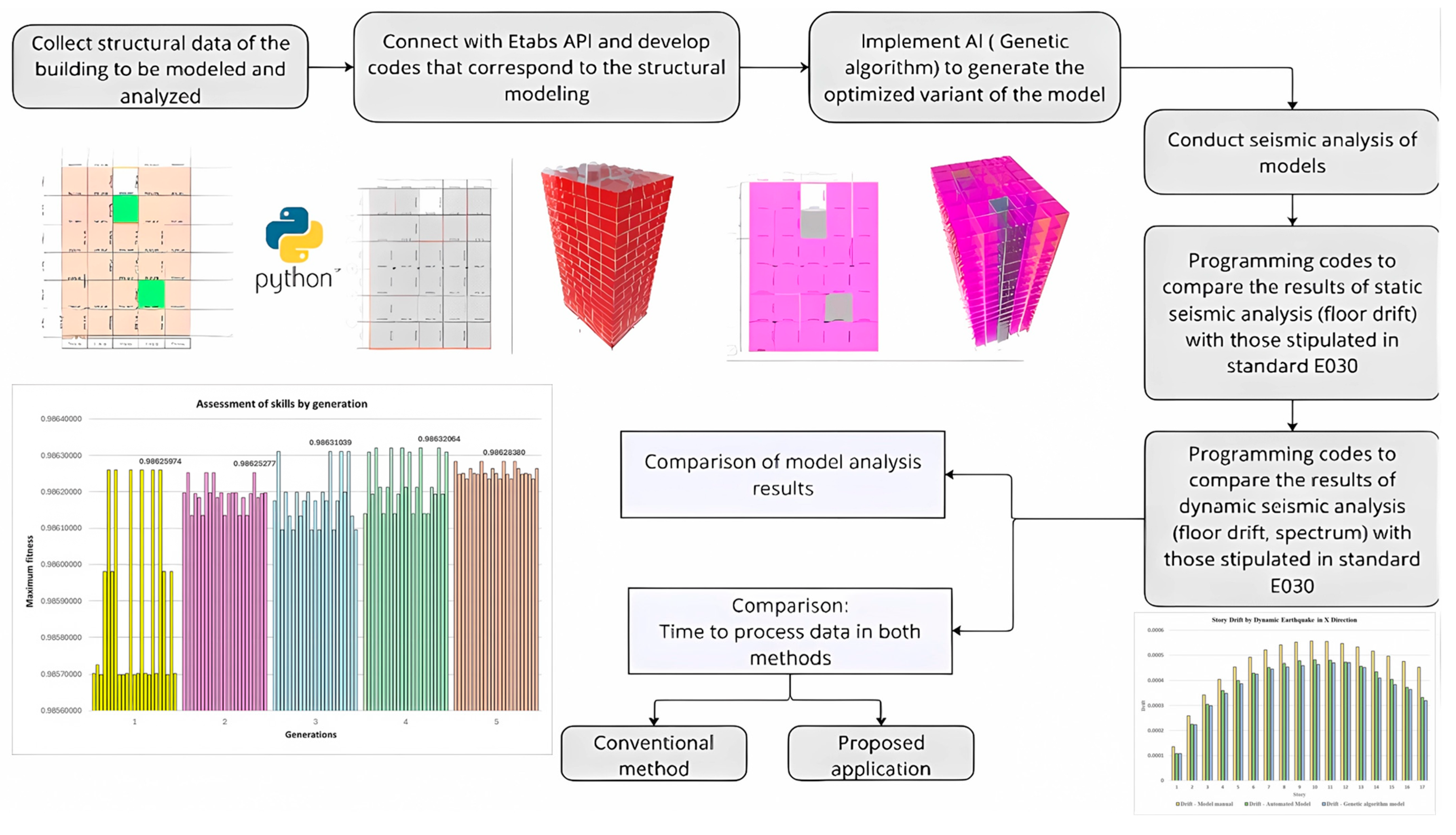
Figure 1 shows the general flow chart of the methodological process proposed in this research. The process begins with the collection of information from the base building, a structure of seventeen regular levels, which includes sections of structural elements, material properties, geometric configuration, and gravitational and seismic loads, among other relevant parameters. These data are organized in an Excel file for further processing.

Figure 1. The proposed workflow.

From the collected data, a code is programmed in Python to automate the complete structural model within the ETABS environment through its API (Application Programming Interface). To provide a clearer view of the ETABS-API implementation, the Python code interacts with ETABS by creating or modifying structural elements programmatically. The workflow includes connecting to an existing ETABS model, defining materials and section properties, creating columns, beams, and walls according to the collected coordinates, applying load patterns, and generating the structural model. Each procedure is executed through specific API calls, ensuring that the geometry, material, and loading conditions of the base building are accurately replicated in the automated model. After the automated model is built, the code validates the model by checking element consistency, connectivity, and load assignment. Then, the correct execution of the process is validated. The resulting base model is used as a starting point to generate an optimal solution using a genetic algorithm.

The optimization algorithm adjusts sections of structural elements, such as columns and beams, using a genetic algorithm-based approach that includes crossing operations and controlled mutation. The columns are adjusted under constraints that ensure that the section of each is equal to or less in area than the previous one, while the beams can vary freely among the available options. Each solution (individual) is evaluated by analyzing the maximum displacement of the structure, using ETABS. The fitness of each individual is calculated as the inverse of this displacement, so that solutions with less displacement (less deformation) are considered better.

The process is repeated across generations, selecting and crossing the best solutions to generate new configurations, while introducing random mutations to explore different combinations. Finally, the best model, that is, the one which generates the smallest displacement, is saved as the optimal solution. After generating the optimal model, a separate Python code was implemented to extract and compare material quantities, such as concrete volumes and steel weights, between the manually created model and the optimized model. This step provides additional quantitative support to evaluate the effects of the genetic algorithm on structural element sizing. Subsequently, a second Python code connects to ETABS through its API to configure both the automated model and the optimized genetic model for static and dynamic seismic analysis. The algorithm then automatically extracts the most relevant results, such as displacements, drifts, internal forces, basal shear, vibration modes, periods, and other key parameters. These results are processed in Python and verified according to the parameters established by current national seismic regulations (E.030).

In addition, a static and dynamic seismic analysis of the traditional structural model is performed, generated directly in ETABS without the optimization process. This analysis is carried out using the same load conditions and structural parameters. By comparing the results obtained from the three methods (traditional, automated with API, and genetic), differences in displacements, internal forces, basal shear, and other factors affecting the seismic behavior of the structure are identified.

Finally, the execution times of the developed algorithms are compared to the average time required by the conventional method of structural modeling and analysis.

3. Mathematical Formulation

This article develops an applied methodology that seeks to automate the structural modeling and seismic analysis of tall reinforced concrete buildings through the implementation of computational algorithms developed in the Python language.

3.1. Modelling in ETABS

Static Analysis

According to Technical Standard E.030 [24], static seismic analysis models the seismic loads by applying a system of forces distributed at the center of mass of each level of the building. This procedure is applicable to the analysis of all structures, whether regular or irregular.

The basic shear force in a specific direction of the structure is calculated using Equation (1).

$$V={\displaystyle \frac{(Z\times U\times C\times S)}{R}}\times P$$

(1)

where

V: Shear force at the base.

Z: Seismic zone coefficient.

U: Factor associated with the use and category of the building.

C: Site coefficient.

S: Seismic amplification coefficient.

R: Seismic response reduction coefficient.

P: Total seismic weight of the building.

3.2. AI Algorithms

3.2.1. Genetic Algorithm

A genetic algorithm (GA) is a search technique used to find exact or approximate solutions to optimization and search problems, inspired by the processes of biological evolution, such as inheritance, mutation, selection, and crossing (also known as recombination). According to Fogel [25], in this approach, a population of abstract representations (called chromosomes or genotypes) of candidate solutions (individuals or phenotypes) evolves into better solutions over several generations.

According to Lie [26], the evolutionary process begins with an initial population of randomly generated individuals. In each generation, the ability of each individual is evaluated according to an optimization criterion. Then, several individuals are selected stochastically according to their fitness and modified through operations such as crossing and mutation, generating a new population. This process is repeated in iterations until an optimal solution, or a satisfactory level of fitness, is achieved.

Cormen et al. [27] comment that the fitness function f(x) is the measure of the quality of a solution x. Generally, this function is sought to maximize. The objective is to find the value of x that optimizes the fitness function, that is, it maximizes f(x). If we have a solution population X = {x₁, x₂, …, x_n}, the algorithm performs the iterations shown in Equation (2).

$$f\left(x_i\right) for each x_i\in X$$

(2)

$f\left(x_i\right)$ is the fitness of the solution $x_i$.

The best individuals (with higher $f\left(x_i\right)$) are more likely to be selected for crossing. Given two parents $x_1 \mathrm{a}\mathrm{n}\mathrm{d} x_2$, the crossing can generate a child x’ using Equation (3).

$$x^{\prime }=Crossing (x_1, x_2)$$

(3)

This may involve combining parts of $x_1$ and $x_2$ to generate new solutions. A mutation with probability pm is applied to alter one of the genes in solution x. The mutation is generated according to Equation (4), which may be a random change in the value of a bit or number on the chromosome.

$$x^{″}=Mutation ({x }^{\prime },p_m)$$

(4)

Finally, the newly generated individuals replace the weaker ones in the population.

3.2.2. Fitness

Fitness in this research is based on the optimization of the maximum displacement of the structure, which is obtained after carrying out seismic analysis in ETABS. Since the aim is to minimize displacements (that is, to achieve a more stable structure), fitness can be defined as the inverse of maximum displacements as seen in Equation (5).

$$Fitness={\displaystyle \frac{1}{Maximum displacement+1}}$$

(5)

3.3. Model Fit Evaluation and Predictive Accuracy

3.3.1. Coefficient of Determination (R²)

Cheng [28] defines the coefficient of determination R² as a statistical measure that evaluates the goodness-of-fit of a linear regression model. Defined as the square of the multiple correlation coefficient between the dependent variable (study variable) and the independent variables (explanatory variables), using observed sample values.

$$R^2=1-{\displaystyle \frac{\sum _{i=1}^n{(y_i-{\widehat{y}}_i)}^2}{\sum _{i=1}^n{(y_i-\overline{y})}^2}}$$

(6)

where

R²: Coefficient of determination. Measures the proportion of the total variability of the dependent variable that is explained by the regression model.

$n$: Total number of observations.

$y_i:$ Observed value of the dependent variable in observation i.

${\widehat{y}}_i:$ Estimated or predicted value by the model for observation i.

$\overline{y:}$ Arithmetic means the observed values of the dependent variable.

3.3.2. Root Mean Squared Error (RMSE)

According to Hodson [29], the Root-Mean-Square Error (RMSE) is a commonly used statistical metric for evaluating the performance of predictive models. Represents the square root of the average error squared between observed and estimated values by the mode.

$$RMSE=\sqrt{{\displaystyle \frac{1}{n}}-\sum _{i=1}^n{(y_i-{\widehat{y}}_i)}^2}$$

(7)

where

$n$: Total number of observations.

$y_i:$ Observed value of the dependent variable in observation i.

${\widehat{y}}_i:$ Estimated or predicted value by the model for observation i.

4. Empirical Assessment of Tall Buildings—Automated Structural Modelling

4.1. Case Study

A theoretical building model of 17 levels was developed, designed for structural simulation and comparative analysis. The building was designed with a regular configuration in plan and height.

The structural system adopted corresponds to a dual system, which combines moment-resistant frames and structural walls, in accordance with the guidelines established in applicable seismic regulations. This configuration allows us to evaluate the response of the model against seismic actions in a representative way.

The model includes the following types of structural elements:

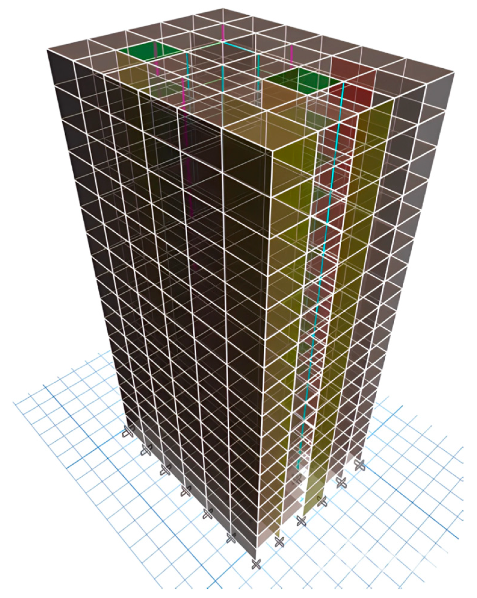
Two main types were considered: column C1, with dimensions of 0.25 m by 0.60 m, and column C2, of 0.30 m by 0.70 m. Both were designed with a concrete compressive strength of f’c = 210 kgf/cm². Reinforced concrete beams are distributed in both longitudinal and transverse directions, connecting columns and transferring loads to the vertical elements. The beam system consists of three types: a beam of 0.25 m by 0.60 m, another one of 0.30 m by 0.60 m, and a flat beam of 0.10 m by 0.10 m. All beams were designed with a concrete strength of f’c = 210 kgf/cm². The structural cut-off walls are located in central areas of the building, simulating vertical circulation cores, with the aim of providing strength and lateral rigidity. Five types of walls were modeled, all with a concrete strength of f’c = 210 kgf/cm², differentiated by their thicknesses: 0.15 m, 0.25 m, 0.28 m, 0.30 m, and 0.40 m. Finally, Story drift was considered, differentiated into lightened slabs for typical floors, in order to optimize the system’s own weight, and solid slabs in specific areas where higher load concentrations or stiffness requirements are expected. This model, as presented in Figure 2 and Figure 3, is a generic representation of mid-rise urban buildings commonly designed in the Latin American context and was used as a basis for evaluating automation methodologies in structural modeling and seismic analysis.

Figure 2. Building modeled on ETABS, different colors represent the structural sections of the elements (columns, beams, and walls).

Figure 3. Building plan modeled on ETABS, different colors indicate the type of structural section, and the labels (e.g., V30x60) correspond to the dimensions and designation of beams.

4.1.1. Seismic Parameters

Seismic Zone (Z)

The city of Lima is located in Seismic Zone 4, defined as a very high seismic hazard area.

Seismic zone: Zone 4.

Z value: 0.45.

Building Use (U)

Multi-family house building corresponds to a usual use without special requirements. U value: 1.0.

Building Category (C)

The proposed building has 17 floors; therefore, it is classified in Category C. This category groups buildings of common use that require detailed seismic design, such as multi-family buildings, offices, hotels, among others.

Structural System

The dual system combines reinforced concrete walls, columns, and beams designed to withstand major seismic forces. This system provides high lateral stiffness, which reduces displacement and deformation during an earthquake. It is commonly used in Lima for buildings of more than 10 floors due to its effectiveness in seismic protection.

4.1.2. Soil and Site Parameters

Soil Type

A soil type S2 (intermediate soil) composed of sandy gravels or dense to very dense sands or consolidated sedimentary deposits shall be considered.

Site Coefficient (C) and Seismic Amplification Coefficient (S)

For soil type S2, the Peruvian Technical Standard E.030 specifies a site coefficient of C = 1.2 and a seismic amplification factor of S = 1.3, which were adopted in the seismic analysis of the building.

4.1.3. Seismic Analysis Parameters

A viscous damping ratio of 5% was adopted for all vibration modes. This value, widely accepted in international seismic design standards and consistent with the Peruvian Technical Standard E.030, represents the typical energy dissipation capacity of reinforced concrete structures under moderate to severe ground motion. The damping was implemented using the classical proportional Rayleigh damping model, which ensures appropriate energy dissipation across the relevant range of structural frequencies.

To account for torsional effects not explicitly modeled, an accidental diaphragm eccentricity of 0.05 was applied to all diaphragms, in accordance with code provisions. This assumption provides a conservative representation of potential irregularities in mass distribution and construction tolerances, improving the reliability of seismic demand estimation.

For the combination of modal responses, the Square Root of the Sum of Squares (SRSS) method was employed. This approach provides an efficient and reliable estimation of maximum structural responses when modal frequencies are sufficiently well separated, which is typically the case for high-rise buildings with dual structural systems. The use of SRSS ensures compliance with seismic design requirements and prevents the underestimation of displacements, drifts, and internal forces arising from multi-modal excitation.

5. Empirical Evaluation of High Buildings—Automated Static Seismic Analysis and Genetic Algorithm

5.1. Derivation Calculation-Static Analysis

The Story drift, which is the relative deformation between two consecutive floors divided by the height of the floor, is represented and serves to evaluate the flexibility or lateral stiffness of the structure against seismic loads.

Figure 4 shows the variation in X-direction Story drifts for floors 1 to 17, obtained by three calculation methods: manual in ETABS, automated with Python and ETABS API, and a genetic algorithm. It is observed that, while the three methods follow a similar trend, there are significant numerical differences in some floors. For example, on the 10th floor, the manually calculated drift was 0.000727, while the automated method returned a value of 0.000685, and the genetic method returned 0.000664, representing a maximum difference of 0.000063 between the manual and genetic methods. In general, it is seen that the drifts tend to increase until the intermediate floors, where they reach their maximum value, and then decrease slightly towards the upper floors, showing a structural behavior consistent with a regular building. Despite the differences, all values are below the standard limit of 0.007 set by E.030.

Figure 4. Story drift by static earthquake in X direction.

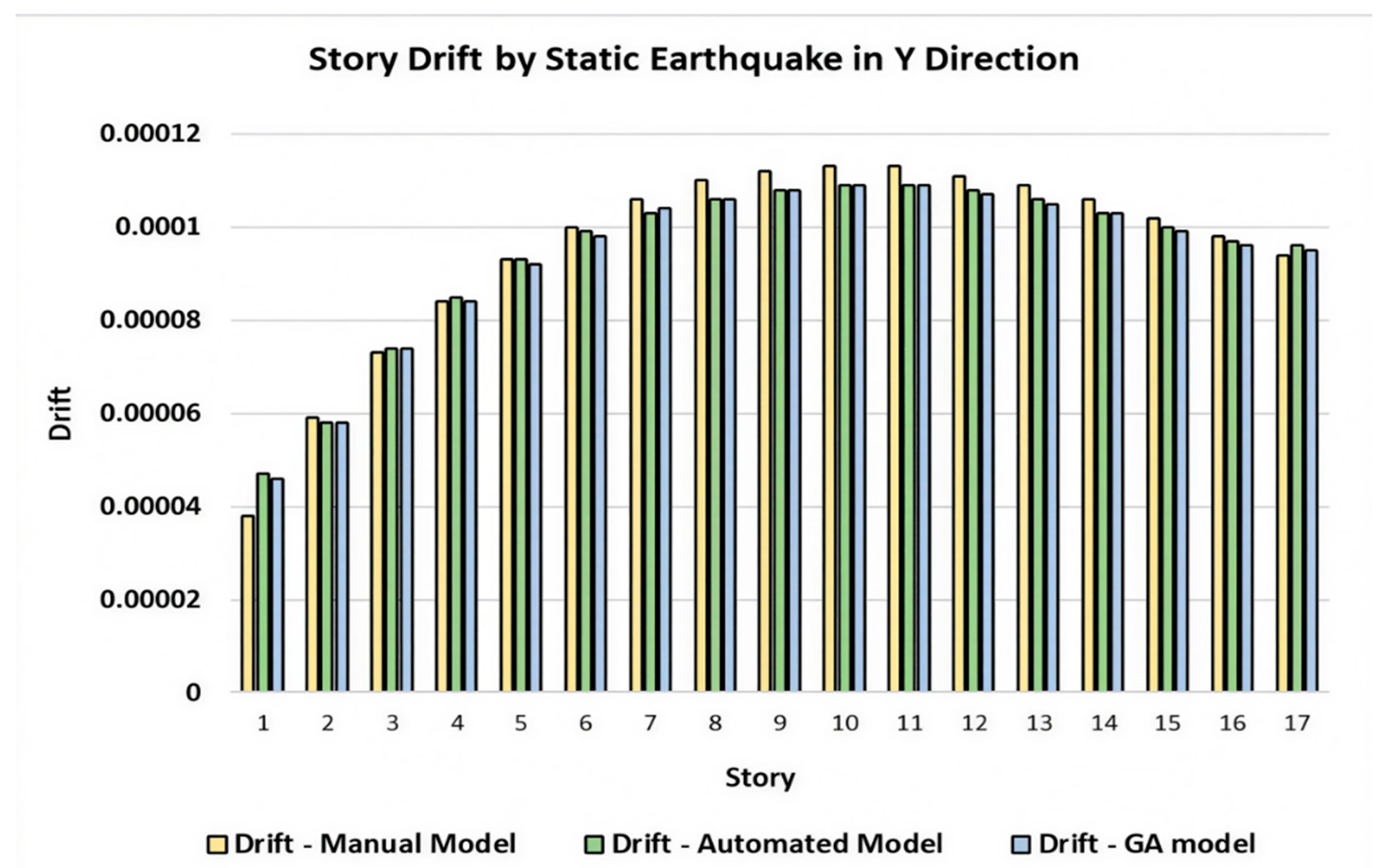
Figure 5 represents the Story drifts for each level in the Y direction under static analysis. Variations are identified between calculation methods. For example, on the 11th floor, the highest drift value was 0.000701 obtained manually, while the automated gave 0.000668 and the genetic 0.000647, generating a difference of 0.000054 between the highest and lowest values. This behavior indicates that while all methods detect the same critical zone in height, the magnitude of drift varies depending on the approach. The drift distribution curve again shows an increasing shape to average levels, which is expected for cumulative displacement, but with technical differences that can be attributed to the rounding, interpolation, or sensitivity parameters of each procedure. Again, all recorded values comply with the drift limit allowed by regulation.

Figure 5. Story drift by static earthquake in Y direction.

The graph in Figure 6 shows the maximum drift per floor along the height of a 17-storey building, with the red curve representing the drift in the Y direction and the blue curve in the X direction. Both curves show how the relative displacement between floors increases with height, being more pronounced in the Y direction. The normative drift limit, set at 0.007 according to the Peruvian Technical Standard E.030 “Sismioresistant Design”, is used as a reference to evaluate structural behavior under lateral loads. In this case, the maximum drifts reached in both directions are much lower than this limit, which indicates a good seismic-resistant performance of the structure, ensuring that the permitted movements between floors are not exceeded and reducing the risk of structural damage.

Figure 6. Maximum drift per floor direction X (blue curve), direction Y (red curve).

Table 1 presents the base reactions obtained in ETABS for the manual, automated, and genetic algorithm models under seismic loads in the X and Y directions (SISMO X and SISMO Y). The results are reported in kN and kN·m for consistency with SI units. For SISMO X, the shear force in the X direction is approximately −4648 kN in all three models, while the corresponding moment in the Y direction is about −143,683 kN·m, reflecting the bending response induced by seismic forces along X. For SISMO Y, the shear force in the Y direction is also around −4648 kN, with an associated moment in the X direction of about 143,683 kN·m, indicating bending about the orthogonal axis due to seismic excitation along Y. As expected, FZ remains zero because vertical seismic forces are not included in this load definition. In contrast, torsional moments MZ are nonzero (ranging from −4692.2148 to 59,761 kN·m depending on the case), accidental eccentricity was applied, and torsional effects were captured. These torsional demands, although present, remain relatively small compared to the dominant bending moments. Overall, the base reaction results confirm the close agreement among the manual, automated, and GA models, with differences on the order of 0.001 tonf (≈0.01 kN), highlighting the consistency of the automated approaches relative to the benchmark manual model.

Table 1. Comparison of base reactions by static loads using the three methods.

Base Reactions—Model Manual
Output Case	Case Type	FX	FY	FZ	MX	MY	MZ
		kN	kN	kN	kN·m	kN·m	kN·m
SISMO X	LinStatic	−4647.6	0	0	0	−143,682.4	59,761.2
SISMO Y	LinStatic	0	−4647.6	0	143,682.6	0	−4692.2148
Base Reactions—Automated Model
Output Case	Case Type	FX	FY	FZ	MX	MY	MZ
		kN	kN	kN	kN·m	kN·m	kN·m
SISMO X	LinStatic	−4647.6	0	0	0	−143,682.3	54,191.0
SISMO Y	LinStatic	0	−4647.6	0	143,682.3	0	−41,807.5
Base Reactions—Genetic algorithm model
Output Case	Case Type	FX	FY	FZ	MX	MY	MZ
		kN	kN	kN	kN·m	kN·m	kN·m
SISMO X	LinStatic	−4647.6	0	0	0	−143,682.3	54,191.0
SISMO Y	LinStatic	0	−4647.6	0	143,682.3	0	−41,807.5

The agreement between the manually modeled and the automated ETABS models was evaluated using per-story static drifts in both X and Y directions. The total number of data points considered was n = 34, corresponding to the number of stories and cases analyzed. The coefficient of determination (R²) and the root mean square error (RMSE) were computed according to Equations (6) and (7), respectively. In this case, R² = 0.9950 and RMSE = 1.9326 × 10⁻⁵, indicating a very high correlation and low error between the automated and manual drift results.

5.2. Genetic Algorithm

This article presents the use of a genetic algorithm to optimize the design of the sections of columns and beams of a structure, with the objective of minimizing the maximum displacement under a seismic analysis performed in the ETABS software. This optimization approach seeks to find the most efficient section configuration, respecting design constraints and structural safety parameters.

The base model used is an ETABS file that describes a standard structure with certain sections of columns and beams. Available sections for columns and beams are pre-defined. To start the optimization process, an initial population of possible solutions is generated. Each “individual” in this population represents a different configuration of column and beam sections, which are randomly assigned within design constraints. This initial population is randomly generated. Each individual in the population is evaluated to determine its performance. This is performed by structural simulation of the model using ETABS software. A seismic analysis is performed to calculate the maximum displacement of the structure under seismic loads. The aim of this step is to minimize displacement, since greater displacement can compromise structural safety.

The fitness of each individual is calculated as the inverse of the maximum displacement. The smaller the shift, the greater the individual’s ability. This fitness is essential for the selection of the most promising individuals for the next generation. To generate a new population, the technique of selection by tournament is used, in which groups of individuals are randomly selected and the best of each group is chosen. The selected individuals are then crossed to generate new “children”. Crossing involves combining the characteristics of two individuals to create a new solution that can inherit the best of both.

Mutation is an additional mechanism that introduces variability in the population and prevents the algorithm from being trapped in sub-optimal solutions. During the mutation process, some sections of columns and beams are changed randomly, with a previously defined probability. This allows you to explore new configurations that might not have been considered initially. The process of selection, crossing, and mutation is repeated over several generations. In each generation, the best individuals are selected to form the next generation. This evolution cycle seeks to gradually improve the solution, focusing on reducing maximum displacement and optimizing structural design.

In this study, the genetic algorithm was configured with a population size of 5 individuals, a total of 5 generations, a mutation probability of 0.1, and a tournament size of 3 for the selection process. These parameters were chosen after preliminary trials to balance solution quality with computational efficiency. Larger populations or alternative settings were tested but led to significantly longer runtimes without improving the results. The adopted configuration allowed the algorithm to converge quickly, showing its best performance around Generation 4, after which the results stabilized, indicating convergence.

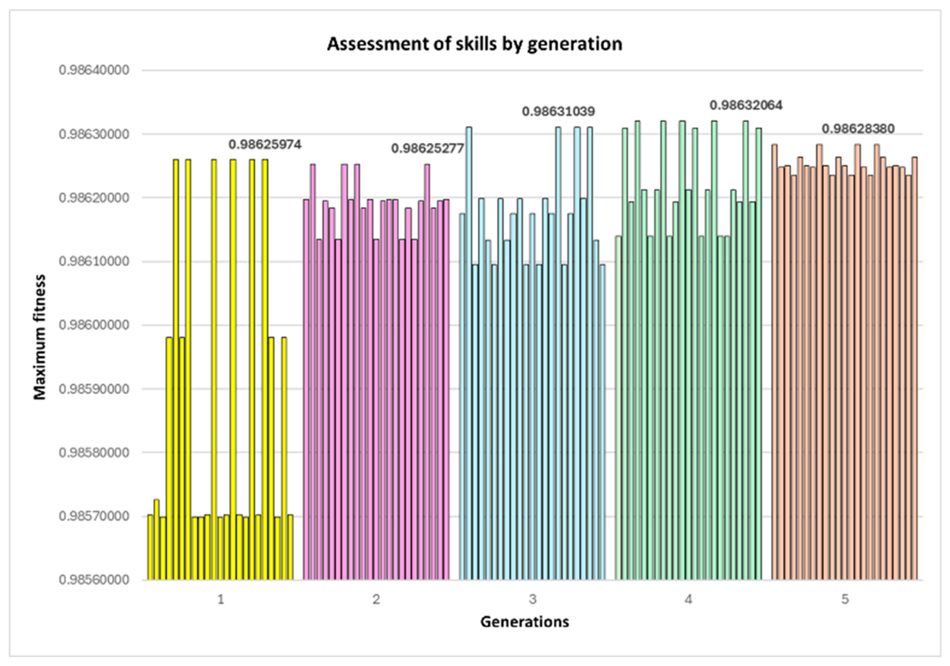
Table 2 shows the results of five generations of the algorithm, with the maximum fit and offset values for each, and Figure 7 shows a graph showing inter-generation improvements. The fitness values remain consistent, ranging from 0.98625974 in the first generation to 0.98628380 in the fifth, while the maximum displacement varies between 0.01393169 in the first generation and 0.01386908 in the fourth, rising slightly to 0.01390696 in the fifth. The best combination of maximum fitness and minimum displacement is found in the fourth generation, with a fitness of 0.98632064 and a displacement of 0.01386908. Therefore, this configuration was selected as the optimal solution due to its balance between fitness and displacement, meeting design and structural safety constraints.

Table 2. Output when running the genetic algorithm.

Generation	Maximum Fitness	Maximum Displacement
1	0.98625974	0.01393169
2	0.98625277	0.01393885
3	0.98631039	0.01387962
4	0.98632064	0.01386908
5	0.98628380	0.01390696

Figure 7. Evolution of skills by generation, numbers 1–5 indicate the corresponding generations.

Table 3 summarizes the comparison between the manual model and the optimized model obtained through the genetic algorithm in terms of concrete volume, steel weight, and the fundamental period of vibration (T₁). Using a dedicated Python code, these quantities were extracted automatically from the ETABS models. The results show slight differences between the manual and optimized models, reflecting the adjustments introduced by the genetic algorithm in structural element sizing.

Table 3. Comparison between manual design and genetic algorithm optimization.

	Manual	Genetic Algorithm	Difference
Concrete volume (m3)	454.57	456.7	+0.47%
Weight of steel (t)	40.37	38.75	−4.01%
Fundamental period T1 (s)	0.459	0.464	+1.09%

6. Empirical Assessment of Tall Buildings—Automated Dynamic Seismic Analysis

Derivation Calculation-Dynamic Analysis

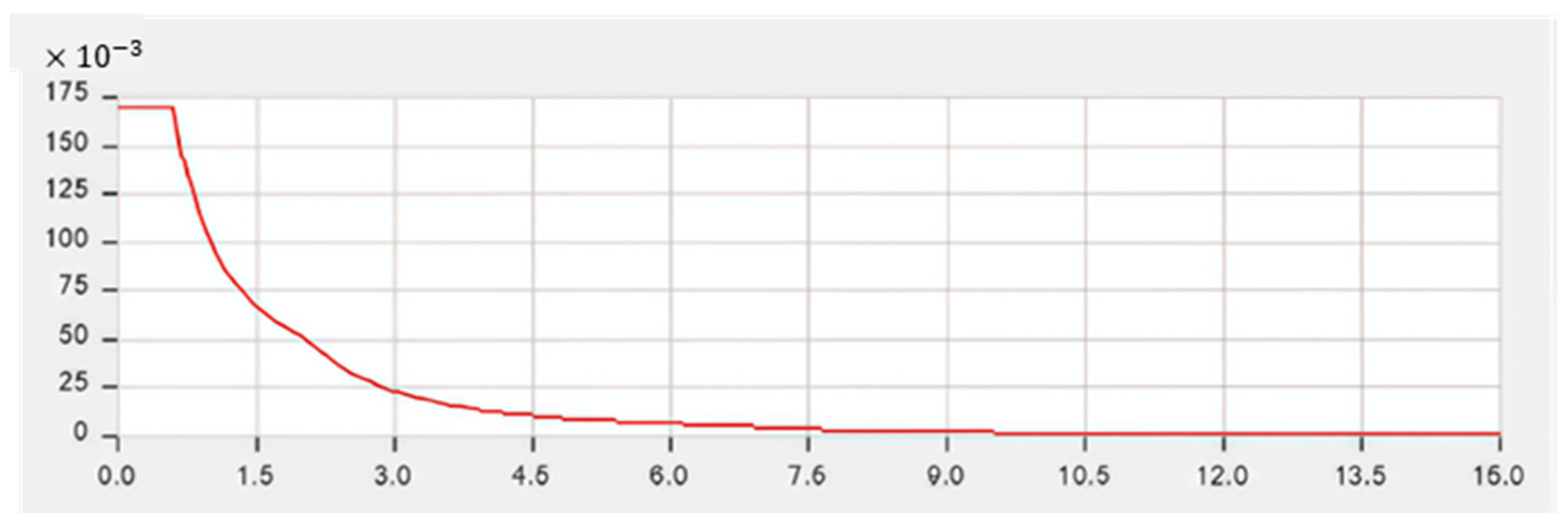
Table 4 shows the relationship between the period of vibration of the structure and its acceleration during a seismic analysis. The period of vibration refers to the time it takes for the structure to complete a cycle of vibration, which is related to the frequency of oscillation of the building. In this context, acceleration indicates how fast the structure moves due to seismic forces. As the period increases, indicating that the structure has a longer vibration cycle and therefore a lower oscillation frequency, the acceleration decreases. This is characteristic of structures that have greater flexibility, since the more rigid structures have a shorter period and respond with higher accelerations. In the table, it is observed that at 0 s (the shortest period), the acceleration is 0.1688, which represents the maximum acceleration observed for the shortest periods of vibration. Then, as the period increases (implying greater flexibility of the structure), the acceleration gradually decreases. For example, at 1 s, the acceleration is 0.1012, and at 5 s, the acceleration is 0.0081, much lower. This behavior is typical of structural systems, where structures with a longer period (more flexible) experience lower accelerations due to lower stiffness. At the end of the table, at 15 s, the acceleration is 0.0009, showing that for very long periods, the structure moves with a very small acceleration. This reflects how the dynamics of the structure change depending on its ability to vibrate, with more flexible structures responding with lower accelerations compared to more rigid ones. This can be demonstrated by the graph in Figure 8.

Table 4. Period of vibration and acceleration of the structure.

Period (Sec.)	Acceleration (m/s2)
0	0.1688
0.1	0.1688
0.2	0.1688
0.3	0.1688
0.4	0.1688
0.5	0.1688
0.6	0.1688
0.7	0.1446
0.8	0.1266
0.9	0.1125
1	0.1012
1.2	0.0844
1.5	0.0675
1.7	0.0596
2	0.0506
2.5	0.0324
3	0.0225
3.5	0.0165
4	0.0127
5	0.008100
8	0.003164
11	0.001674
15	0.000900

Figure 8. Design response spectrum extracted from ETABS.

Figure 9 corresponds to the dynamic analysis by spectral response in the X direction. It is observed that the 10th floor presents the maximum drift for all three methods: the manual value was 0.000557, the automated value of 0.000482, and the genetic 0.000464, which reflects a difference of 0.000093 between the manual and the genetic method. Although the overall shape of the curve is consistent, with greater drift in the mean levels, differences between methods are more marked than in static analysis, due to the nature of spectral analysis and its sensitivity to modal participation and mass distribution. These differences show that the use of artificial intelligence and automation can slightly alter the prediction of seismic behavior, but without compromising structural safety, as all values are well below the 0.007 limit.

Figure 9. Story drift by dynamic earthquake in X direction.

Figure 10 shows the results of the drift under dynamic analysis in the Y direction. In this case, the maximum drift is also detected on the 10th floor, with values of 0.000504 for the manual method, 0.000456 for the automated, and 0.000437 for the genetic, generating a maximum difference of 0.000067. Although the curves are similar in form, it is evident that the genetic algorithm tends to offer lower values than the traditional method. This is related to the way in which the algorithm optimizes the input parameters or the effective rigidity of the model. In all cases, the structural behavior remains within acceptable ranges, and the regulatory limit value is met, ensuring that the building does not present problems of excessive deformation due to dynamic seismic action.

Figure 10. Story drift by dynamic earthquake in Y direction.

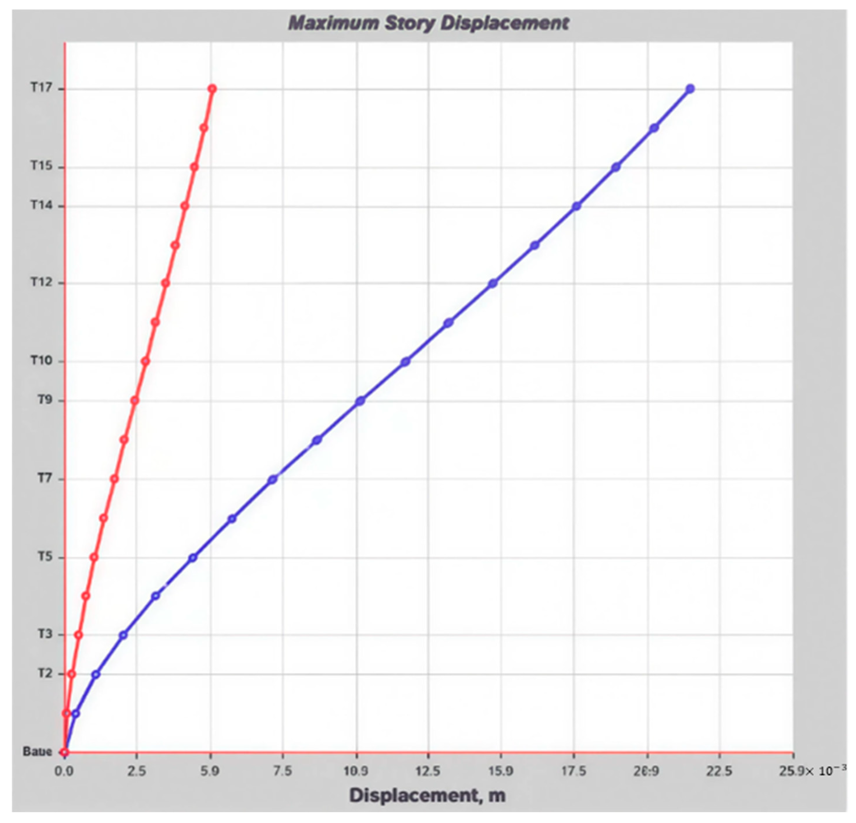
Figure 11 shows the displacement (m), which represents the maximum displacement in meters for each floor of the structure. The displacement values are small, lo., indicating a moderate structural behavior in terms of displacements. The red curve represents the drift of the upper floors under seismic action in the X direction (usually horizontal). This curve shows that the displacement in the upper floors increases as the intensity of the seismic load increases. The blue curve shows the displacement of the floors at the base of the structure, with an almost linear behavior relative to the base (greater displacement as floors increase).

Figure 11. Maximum drift per floor X direction (red curve), Y direction (blue curve).

Table 5 shows the results of the Modal Participant Mass Ratio for a 17-storey building, considering a total of 51 cases corresponding to three vibration modes per floor. Each case represents a specific vibration mode, which describes how the building moves under an external force, such as an earthquake, and each mode reflects a unique movement pattern. The “Mode” indicates the vibration mode, while the “Period” is the time it takes for the building to perform a complete oscillation cycle. A shorter period is associated with a higher vibration frequency, which means that the structure will move faster, while a longer period implies a slower vibration.

Table 5. Modal participant mass ratios in response to vibration.

Case	Mode	Period	UX	UY	UZ	RX	RY	RZ
MODAL	1	0.459	0.6304	0.0000183	0	0.00001025	0.2749	0.0652
MODAL	2	0.205	0.0001	0.7019	0	0.297	0.00000421	0.00001437
MODAL	3	0.118	0.1508	0.00001219	0	0	0.342	0.0287
MODAL	4	0.104	0.0851	0.00003778	0	0.00001247	0.0124	0.6906
MODAL	5	0.056	0.0479	0.000007918	0	0.0000116	0.1087	0.006
MODAL	6	0.054	0	0.1894	0	0.4045	0.000001291	0.00001382
MODAL	7	0.036	0.0256	0	0	0	0.0729	0.0008
MODAL	8	0.033	0.0113	0.000004556	0	0.00001856	0.0444	0.124
MODAL	9	0.027	5.491 × 10−7	0.0488	0	0.1167	0.000001345	0
MODAL	10	0.026	0.0132	6.968 × 10−7	0	0.000002027	0.0368	0.0017
MODAL	11	0.02	0.0092	0	0	0	0.0274	0.0006
MODAL	12	0.018	0.0031	0.00001009	0	0.00003838	0.0073	0.0346
MODAL	13	0.018	0.000002175	0.023	0	0.0687	0.000003717	0.00003222
MODAL	14	0.016	0.006	0	0	0	0.0178	0.0007
MODAL	15	0.014	0.0043	0	0	0	0.0134	0.0004
MODAL	16	0.013	9.161 × 10−7	0.0128	0	0.0371	0.000002954	0.00001181
MODAL	17	0.013	0.0017	0.00001719	0	0.0001	0.0063	0.0167
MODAL	18	0.012	0.0028	0	0	0	0.0086	0.0006
MODAL	19	0.011	0.0023	0.000000607	0	0.000002041	0.0073	0.0001
MODAL	20	0.011	0	0.008	0	0.0252	0	0.000005205
MODAL	21	0.01	0.0007	0.000007973	0	0.00002331	0.002	0.0097
MODAL	22	0.01	0.0016	0	0	0	0.005	0.0001
MODAL	23	0.009	0.000002933	0.0052	0	0.016	0.000008988	0.000002463
MODAL	24	0.009	0.001	0.000006552	0	0.00001994	0.0033	0.0002
MODAL	25	0.008	0.0008	0	0	0	0.0026	6.015 × 10−7
MODAL	26	0.008	0.0003	0.000006353	0	0.00002113	0.0013	0.0062
MODAL	27	0.008	0.0005	0	0	0	0.0015	0.00001332
MODAL	28	0.008	0	0.0036	0	0.0115	0.00000167	0.000004874
MODAL	29	0.008	0.0002	0	0	0	0.0007	0.00004932
MODAL	30	0.007	0.0001	0	0	0	0.0004	0.000002108
MODAL	31	0.007	0.00002342	0	0	0	0.0001	0.000005299
MODAL	32	0.007	0.0003	0.0003	0	0.001	0.0007	0.0036
MODAL	33	0.007	0.0000355	0.0021	0	0.0067	0.0001	0.0005
MODAL	34	0.006	0	0.0017	0	0.0056	0	0
MODAL	35	0.006	0.0002	0	0	8.187 × 10−7	0.0007	0.0028
MODAL	36	0.006	0	0.0012	0	0.0038	0	5.101 × 10−7
MODAL	37	0.005	0.0001	0.00000179	0	0.000005919	0.0004	0.002
MODAL	38	0.005	0	0.0008	0	0.0026	7.794 × 10−7	0.000004315
MODAL	39	0.005	0	0.0005	0	0.0016	0	0
MODAL	40	0.005	0.0001	0	0	0	0.0003	0.0014
MODAL	41	0.005	0	0.0003	0	0.001	0	0
MODAL	42	0.005	0	0.0002	0	0.0005	0	0
MODAL	43	0.005	0	0.0001	0	0.0002	0	0.000001602
MODAL	44	0.005	0.0001	5.538 × 10−7	0	0.000001691	0.0002	0.0009
MODAL	45	0.005	0.000001657	0.000006002	0	0.00001654	0.000004974	0.00002619
MODAL	46	0.004	0.00004018	0	0	0	0.0002	0.0007
MODAL	47	0.004	0.00002488	0	0	0	0.0001	0.0004
MODAL	48	0.004	0.00001414	0	0	0	0.0001	0.0002
MODAL	49	0.004	0.000006673	0	0	0	0.00001775	0.0001
MODAL	50	0.004	0.000001994	0	0	0	0.000008984	0.00003575
MODAL	51	0.004	0	0	0	0	9.394 × 10−7	0

For displacements in the X, Y, and Z directions (represented by the columns UX, UY, and UZ), the ranges of displacements of each floor in each of these directions are shown. For example, in MODAL 1, the value of UX = 0.6304 indicates a significant shift in the X-direction, which is characteristic of vibration modes where seismic force mainly affects that direction. On the other hand, UY = 0 and UZ = 0 indicate that there is no displacement in the directions Y and Z in this mode. This behavior is common in early vibration modes, where vibrations tend to concentrate in one or two main directions, leaving other directions without impact.

In addition, the columns RX, RY, and RZ reflect the rotations of the building around the X, Y, and Z axes, respectively. In MODAL 1, the value RX = 0.00001025 shows a small rotation around the X-axis, implying that although there is some spin, the rotation is minimal compared to the displacement. Rotation values are generally small in the first modes, suggesting that the structure is more displaced than rotated in those specific vibration modes. A near-zero values in RX, RY, or RZ indicate that the rotation in that direction is minimal or negligible, which means that the vibration mode has no significant impact on the rotations of the building.

These results are essential to understand how each floor of the structure moves and rotates under dynamic loads such as those caused by an earthquake. Displacement and rotation values in each vibration mode allow engineers to identify the predominant directions of motion and adjust the structural design to mitigate resonance effects and improve the building’s resistance to vibration. In this way, informed decisions can be made on the reinforcement and optimization of the structure to ensure safety and stability against seismic forces.

Table 6 presents the results of a spectral response analysis (LinRespSpec) carried out on the proposed 17-storey building to evaluate its behavior under seismic forces in the X and Y directions. This analysis reports the shear forces (FX, FY, FZ) and bending moments (MX, MY, MZ) acting on the structure. The results indicate that in FX, the shear force in the X direction varies between 3159 kN in the manual case, 2697 kN in the automated case, and 2706 kN in the genetic case, with the maximum value corresponding to the manual analysis, reflecting how the structure reacts to horizontal seismic forces in that direction. In FY, the shear force in the Y direction reaches 3466 kN in the manual case, 2959 kN in the automated case, and 2962 kN in the genetic case, indicating the response of the structure to seismic loads in the Y direction. The force FZ is 0 in all cases, which means that no vertical load is being considered in this analysis, as the focus is on the lateral behavior of the structure. As for the bending moments, the MX values show significant bending in the X direction, with 1133 kN·m in the manual case, 1101 kN·m in the automated case, and 1814 kN·m in the genetic case, with the maximum value being that of the genetic analysis, indicating that the structure is experiencing bending in this direction due to seismic forces. In MY, bending moments in the Y direction are also relevant, with 97,997 kN·m in the manual case, 85,772 kN·m in the automated case, and 84,355 kN·m in the genetic case, showing that the structure flexes in the Y direction but with a smaller magnitude compared to the X direction. Finally, the torsional moments MZ in the Z direction are nonzero, reaching values of 48,486 kN·m in the manual case, 39,297 kN·m in the automated case, and 38,692 kN·m in the genetic case for SDx, and about 34,121 kN·m (manual), 26,434 kN·m (automated), and 26,264 kN·m (genetic) for SDy. These results confirm that torsion was considered, although its effect remains modest compared with the dominant flexural response, and that the main focus of this analysis is the lateral performance of the structure under seismic loading in the X and Y directions.

Table 6. Comparison of base reactions by static loads using three methods.

Base Reactions—Model Manual
Output Case	Case Type	FX	FY	FZ	MX	MY	MZ
		kN	kN	kN	kN·m	kN·m	kN·m
SDx	LinRespSpec	3159.329	35.335	0	1132.934	97,996.780	48,485.613
SDy	LinRespSpec	35.335	3466.030	0	107,739.918	982.624	34,121.209
Base Reactions—Automated Model
Output Case	Case Type	FX	FY	FZ	MX	MY	MZ
		kN	kN	kN	kN·m	kN·m	kN·m
SDx	LinRespSpec	2697.420	34.004	0	1100.929	85,771.947	39,296.772
SDy	LinRespSpec	34.005	2959.197	0	92,254.261	944.555	26,434.123
Base Reactions—Genetic algorithm model
Output Case	Case Type	FX	FY	FZ	MX	MY	MZ
		kN	kN	kN	kN·m	kN·m	kN·m
SDx	LinRespSpec	2705.823	56.131	0	1814.233	84,355.035	38,691.561
SDy	LinRespSpec	56.131	2961.589	0	92,315.328	1523.735	26,263.629

The agreement between the manually modeled and the automated ETABS models was evaluated using per-story dynamic drifts in both X and Y directions. The total number of data points considered was n = 34, corresponding to the number of stories and cases analyzed. The coefficient of determination (R²) and the root mean square error (RMSE) were computed according to Equations (6) and (7), respectively. In this case, R² = 0.9385 and RMSE = 5.2174 × 10⁻⁵, indicating a very high correlation and low error between the automated and manual drift results.

7. Discussions

The results obtained in Figure 4 and Figure 5, which present the story drifts of static analyses performed with the traditional model and the automated model using the ETABS API, demonstrate a significant improvement in accuracy with the automated approach. The value of R² = 0.9950 indicates that the automated model explains 99.5% of the variability of the manual results, reflecting an almost perfect fit. Furthermore, the RMSE = 1.93 × 10⁻⁵ is extremely low, reinforcing the conclusion that the difference between both approaches is practically negligible and that the automated model successfully replicates the structural response under static seismic loading.

As for the dynamic drift analysis presented in Figure 9 and Figure 10, the automated model with API also shows excellent precision in estimating structural behavior under seismic conditions. The determination coefficient of R² = 0.9385 confirms that 93.85% of the observed variability in interstory drifts is explained by the model, reflecting a very good fit relative to the traditional approach. Likewise, the RMSE = 5.22 × 10⁻⁵ highlights the very small error magnitude and validates the automated framework as a reliable alternative for dynamic response estimation.

It is important to note, however, that these validation metrics correspond exclusively to the case study of a 17-story dual system building.

In terms of runtime, the automated model with API shows a marked advantage over the manual procedure. At the same time, traditional modeling and analysis in ETABS takes approximately three hours, the automated workflow completes the entire process in just 13.2 min, representing a 99.5% reduction in computational time. This time includes static and dynamic seismic modeling, structural analysis, and the extraction of result tables, underscoring the high efficiency of the automated approach.

On the other hand, the use of the genetic algorithm (GA) required an execution time of 191 min, reflecting the complexity and iterative nature of the optimization process. Unlike the automated model, which performs rapid and straightforward simulations, the GA involves a stochastic search requiring the evaluation of multiple generations of models to find an optimal solution. Nevertheless, this runtime remains practical considering the scale of the 17-story dual system analyzed and the large number of ETABS evaluations involved. Moreover, parameter tuning, parallel processing, or the use of more advanced hardware could further reduce computation time. Thus, the principal contribution of this study lies in demonstrating the feasibility of optimization through GA, rather than minimizing runtime.

In addition to drift-based validation, it is essential to evaluate the material and dynamic consequences of the optimization framework. Table 3 summarizes the comparative results between the baseline manual model and the GA-optimized solution in terms of total concrete volume, reinforcement weight, and fundamental period (T₁). The results indicate that the GA model requires a slightly higher volume of concrete (+0.47%) but achieves a noticeable reduction in reinforcement demand (−4.01%) when compared with the manual design. This redistribution of material demand suggests that the optimization framework improves efficiency by marginally increasing concrete use while significantly reducing reinforcement tonnage, which may translate into cost benefits in scenarios where reinforcement represents the dominant structural expense.

With respect to structural dynamics, the fundamental period increased slightly from 0.459 s in the manual model to 0.464 s in the GA solution (+1.09%). This small variation confirms that the optimized design maintains a global stiffness level comparable to that of the baseline structure. From a practical standpoint, the marginal increase in T₁ does not alter the seismic demand classification of the building but does reflect a subtle shift toward greater flexibility, consistent with the reduction in reinforcement.

Finally, the performance of the genetic algorithm across generations, illustrated in Figure 7, shows a clear trend of progressive improvement followed by convergence. The value of R² = 0.3613 suggests that only 36.13% of the variability in performance is explained by the number of generations, which indicates a moderate relationship. Even so, the GA exhibited significant improvement between Generation 1 and Generation 2. Subsequent generations improved more gradually, reaching convergence by Generation 5. The slight decline observed in the last generation suggests that the algorithm reached its maximum level of optimization under the established conditions.

8. Conclusions

The methodology showed an almost perfect correspondence with the manual procedure, achieving R² = 0.995 and RMSE = 0.0006 in static analysis, and R² = 0.9385 with RMSE = 0.032 in dynamic analysis.

Significant reduction in processing time: The automated workflow reduced modeling and analysis time by 99.5%, from approximately three hours in the traditional method to only 13.2 min, without any loss of accuracy.

The incorporation of evolutionary techniques enabled the exploration of more efficient design configurations, achieving a 4.01% reduction in steel consumption at the cost of a minimal increase in concrete (+0.47%). This represents a favorable balance in both structural and economic terms.

All results obtained remained within the limits established by the Peruvian Seismic Design Code (NTP E.030). In particular, interstory drifts remained well below the maximum regulatory threshold of 0.007, reaffirming that automation and optimization do not compromise structural safety.

The integration of the ETABS API with Python programming and optimization techniques provides an innovative framework capable of enhancing accuracy, drastically reducing analysis time, and facilitating the exploration of alternative design solutions. This represents a valuable contribution to both professional practice and applied research in earthquake engineering.

References

- Aloisio, A.; Santis, Y.; De Irti, F.; Pasca, D.P.; Scimia, L.; Fragiacomo, M. Machine learning predictions of code-based seismic vulnerability for reinforced concrete and masonry buildings: Insights from a 300-building database. Eng. Struct. 2024, 301, 117295. [Google Scholar] [CrossRef]
- Angelucci, G.; Quaranta, G.; Mollaioli, F.; Kunnath, S.K. Interpretable machine learning models for displacement demand prediction in reinforced concrete buildings under pulse-like earthquakes. J. Build. Eng. 2024, 95, 110124. [Google Scholar] [CrossRef]
- Asgarkhani, N.; Kazemi, F.; Jakubczyk-Gałczyńska, A.; Mohebi, B.; Jankowski, R. Seismic response and performance prediction of steel buckling-restrained braced frames using machine-learning methods. Eng. Appl. Artif. Intell. 2024, 128, 107388. [Google Scholar] [CrossRef]
- Chen, C.S. Optimization of the seismic resistance of school buildings using artificial intelligence and sensitivity analysis theories—A Taiwan case study. Structures 2023, 54, 857–868. [Google Scholar] [CrossRef]
- Cosgun, C. Machine learning for the prediction of evaluation of existing reinforced concrete structures performance against earthquakes. Structures 2023, 50, 1994–2003. [Google Scholar] [CrossRef]
- De Iuliis, M.; Miceli, E.; Castaldo, P. Machine learning modelling of structural response for different seismic signal characteristics: A parametric analysis. Appl. Soft Comput. 2024, 164, 112026. [Google Scholar] [CrossRef]
- Demertzis, K.; Kostinakis, K.; Morfidis, K.; Iliadis, L. An interpretable machine learning method for the prediction of R/C buildings’ seismic response. J. Build. Eng. 2023, 63, 105493. [Google Scholar] [CrossRef]
- Ekmen, A.B.; Avci, Y. Development of novel artificial intelligence functions based on 3D finite element method using February 6 Kahramanmaraş Seismic Records for earthquake effects prediction in various soils. Eng. Geol. 2024, 336, 107570. [Google Scholar] [CrossRef]
- Falcone, R.; Ciaramella, A.; Carrabs, F.; Strisciuglio, N.; Martinelli, E. Artificial neural network for technical feasibility prediction of seismic retrofitting in existing RC structures. Structures 2022, 41, 1220–1234. [Google Scholar] [CrossRef]
- Gu, Z.; Lu, W.; Fan, Y.; Gao, Y. Automated simplified structural modeling method for megatall buildings based on genetic algorithm. J. Build. Eng. 2023, 77, 107485. [Google Scholar] [CrossRef]
- Ju, S.; Jia, J.; Pan, X. Prediction framework of slope topographic amplification on seismic acceleration based on machine learning algorithms. Eng. Appl. Artif. Intell. 2024, 133, 108143. [Google Scholar] [CrossRef]
- Kazemi, F.; Asgarkhani, N.; Jankowski, R. Machine learning-based seismic response and performance assessment of reinforced concrete buildings. Arch. Civ. Mech. Eng. 2023, 23, 94. [Google Scholar] [CrossRef]
- Kazemi, F.; Asgarkhani, N.; Jankowski, R. Optimization-based stacked machine-learning method for seismic probability and risk assessment of reinforced concrete shear walls. Expert Syst. Appl. 2024, 255, 124897. [Google Scholar] [CrossRef]
- Luo, H.; Paal, S.G. Artificial intelligence-enhanced seismic response prediction of reinforced concrete frames. Adv. Eng. Inform. 2022, 52, 101568. [Google Scholar] [CrossRef]
- Ma, C.; Chi, J.W.; Kong, F.C.; Zhou, S.H.; Lu, D.C.; Liao, W.Z. Prediction on the seismic performance limits of reinforced concrete columns based on machine learning method. Soil Dyn. Earthq. Eng. 2024, 177, 108423. [Google Scholar] [CrossRef]
- Nair, D.S.; Mol, M.B. Enhancing seismic performance prediction of RC frames using MFF-ANN model approach. Multimed. Tools Appl. 2024, 83, 42285–42318. [Google Scholar] [CrossRef]
- Parisi, F.; Ruggieri, S.; Lovreglio, R.; Fanti, M.; Uva, G. On the use of mechanics-informed models to structural engineering systems: Application of graph neural networks for structural analysis. Structures 2024, 59, 105712. [Google Scholar] [CrossRef]
- Stefanini, L.; Badini, L.; Mochi, G.; Predari, G.; Ferrante, A. Neural networks for the rapid seismic assessment of existing moment-frame RC buildings. Int. J. Disaster Risk Reduct. 2022, 67, 102677. [Google Scholar] [CrossRef]
- Wang, T.; Li, H.; Noori, M.; Ghiasi, R.; Kuok, S.C.; Altabey, W.A. Probabilistic Seismic Response Prediction of Three-Dimensional Structures Based on Bayesian Convolutional Neural Network. Sensors 2022, 22, 3775. [Google Scholar] [CrossRef]
- Wen, W.; Zhang, C.; Zhai, C. Rapid seismic response prediction of RC frames based on deep learning and limited building information. Eng. Struct. 2022, 267, 114638. [Google Scholar] [CrossRef]
- Xu, W.; Zhao, Y.; Yang, W.; Yu, D.; Zhao, Y. Seismic fragility analysis of RC frame structures based on IDA analysis and machine learning. Structures 2024, 65, 106774. [Google Scholar] [CrossRef]
- Zhang, T.; Xu, W.; Wang, S.; Du, D.; Miao, Q. Study on the evolution of dynamic characteristics and seismic damage of a self-centering concrete structure based on data-driven methods. Eng. Struct. 2024, 316, 118529. [Google Scholar] [CrossRef]
- Zhang, T.; Xu, W.; Wang, S.; Du, D.; Tang, J. Seismic response prediction of a damped structure based on data-driven machine learning methods. Eng. Struct. 2024, 301, 117264. [Google Scholar] [CrossRef]
- E.030; Reglamento Nacional de Edificaciones: Diseño Sismorresistente. Ministerio de Vivienda, Construcción y Saneamiento: Lima, Peru, 2020.
- Fogel, D.B. Evolutionary Computation: Toward a New Philosophy of Machine Intelligence, 3rd ed.; IEEE Press: New York, NY, USA; Wiley-Interscience: Hoboken, NJ, USA, 2005. [Google Scholar] [CrossRef]
- Lie, L. Heuristic Artificial Intelligent Algorithm for Genetic Algorithm. In Proceedings of the 2010 International Conference on Advanced Measurement and Test (AMT 2010), Sanya, China, 15–16 May 2010; Volume 439–440, pp. 516–521. [Google Scholar] [CrossRef]
- Cormen, T.H.; Leiserson, C.E.; Rivest, R.L.; Stein, C. Introduction to Algorithms, 3rd ed.; The MIT Press: Cambridge, MA, USA, 2009; Available online: https://mitpress.mit.edu/9780262033848/introduction-to-algorithms/ (accessed on 25 September 2025).
- Cheng, C.-L.; Shalabh; Garg, G. Coefficient of determination for multiple measurement error models. J. Multivar. Anal. 2014, 126, 137–152. [Google Scholar] [CrossRef]
- Hodson, T.O. Root-mean-square error (RMSE) or mean absolute error (MAE): When to use them or not. Geosci. Model Dev. 2022, 15, 5481–5487. [Google Scholar] [CrossRef]
Disclaimer/Publisher’s Note: The statements, opinions and data contained in all publications are solely those of the individual author(s) and contributor(s) and not of MDPI and/or the editor(s). MDPI and/or the editor(s) disclaim responsibility for any injury to people or property resulting from any ideas, methods, instructions or products referred to in the content. |
© 2025 by the authors. Licensee MDPI, Basel, Switzerland. This article is an open access article distributed under the terms and conditions of the Creative Commons Attribution (CC BY) license (https://creativecommons.org/licenses/by/4.0/).