Article

Spatial and Data-Driven Approaches for Mitigating Urban Heat in Coastal Cities

1
School of Design, The Hong Kong Polytechnic University, Hong Kong 999077, China
2
School of Architecture, Tianjin Chengjian University, Tianjin 300384, China
*
Author to whom correspondence should be addressed.
Buildings 2025, 15(19), 3544; https://doi.org/10.3390/buildings15193544
Submission received: 2 September 2025 / Revised: 19 September 2025 / Accepted: 23 September 2025 / Published: 2 October 2025
(This article belongs to the Section Architectural Design, Urban Science, and Real Estate)

Abstract

With accelerating urbanization and global climate warming, Urban Heat Islands (UHIs) pose serious threats to urban development. Existing UHI research mainly focuses on inland regions, lacking systematic understanding of coastal city heat island mechanisms. We selected eight Chinese coastal cities with different backgrounds, quantitatively assessed urban heat island intensity based on summer 2023 Landsat 8 remote sensing data, established block-LCZ spatial analysis units, and employed a combination of machine learning models and causal inference methods to systematically analyze the regional differentiation characteristics of Urban Heat Island Intensity (UHII) and the influence mechanisms of multi-dimensional driving factors within land–sea interaction contexts. The results revealed the following: (1) UHII in the study area presents obvious spatial differentiation, with the highest value occurring in Hong Kong (2.63 °C). Northern cities generally had higher values than southern ones. (2) Different Local Climate Zone (LCZ) types show significant differences in thermal contributions, with LCZ2 (compact midrise) blocks presenting the highest UHII values in most cities, while LCZ G (water) and LCZ A (dense trees) blocks exhibit stable cooling effects. Nighttime light (NTL) and distance to sea (DS) are dominant factors affecting UHII, with NTL marginal effect curves generally presenting hump-shaped characteristics, while DS shows different response patterns across cities. (3) Causal inference reveals true causal driving mechanisms beyond correlations, finding that causal effects of key factors exhibit significant spatial heterogeneity. The research findings provide a new cognitive framework for understanding the formation mechanisms of thermal environments in Chinese coastal cities and offer a quantitative basis for formulating regionalized UHI mitigation strategies.

1. Introduction

United Nations statistics show that the global urban population proportion exceeded 55% in 2018 and is expected to reach 68% by 2050 [1]. The acceleration of urbanization has led to large amounts of natural surfaces being replaced by buildings and impermeable surfaces, significantly altering urban surface energy balance and forming Urban Heat Islands (UHIs). UHI refers to the phenomenon where urban areas have significantly higher temperatures than their surrounding suburban areas. UHIs bring serious health risks, potentially causing heat stroke, respiratory diseases, and cardiovascular diseases [2]. Additionally, UHI is closely related to increased energy consumption and deteriorating air quality [3,4]. Therefore, there is an urgent need to formulate and implement effective UHI mitigation strategies.
In-depth understanding of UHI’s multifaceted driving mechanisms is an important prerequisite for formulating scientific mitigation strategies. Existing research shows that UHI formation results from the comprehensive interaction of multiple factors, including biophysical parameters, built environment characteristics, landscape patterns, geographical environment, and socioeconomic dimensions. Biophysical parameters have fundamental impacts on urban thermal environments. Albedo (ALB) directly regulates surface energy balance by affecting the reflection ratio of solar radiation, with lower ALB leading to more solar energy being absorbed by the surface, thereby intensifying UHIs [5]. Vegetation, as an important component of urban ecosystems, significantly affects urban thermal environments through evapotranspiration, shading effects, and radiation regulation mechanisms. The Normalized Difference Vegetation Index (NDVI) is widely used to quantify vegetation coverage and vegetation quality, with research showing significant negative correlations between NDVI and land surface temperature [6,7]. Built environment characteristics are key regulatory factors for UHI. Building density and building height, as core indicators of urban spatial morphology, have been proven by many studies to have multiple impacts on urban thermal environments [8,9,10,11]. Sky View Factor (SVF), as an important parameter reflecting the degree of sky openness, shows complex nonlinear response relationships with UHIs [12,13]. Landscape pattern indicators reveal urban thermal environment formation mechanisms from spatial configuration perspectives. Shape and distribution differences in landscape elements affect energy exchange patterns and efficiency between patches, thereby regulating surface heat flux distribution [14]. Edge density, patch density, and landscape shape index are used to characterize urban landscape patterns to analyze their regulatory effects on urban thermal environments [15,16]. Geographical environmental factors provide important spatial background for UHI research. For coastal cities, distance from sea (DS) serves as a key indicator reflecting ocean cooling effects and has been proven by multiple studies to be a crucial factor affecting Urban Heat Island Intensity (UHII) [17,18,19]. Socioeconomic factors reflect the important influence of human activities on UHI. Population Density (PD) and Nighttime Light (NTL), as proxy indicators reflecting human activity intensity, are both closely related to urban thermal environments [20,21].
Despite our increasing understanding of the driving mechanisms of UHIs, there is still a clear bias in the selection of research regions. Through a systematic analysis of relevant literature in recent years, it was found that most studies utilized inland metropolises as their research areas, such as Beijing [22], Xi’an [23,24], Chengdu [25,26], etc., with relatively few studies emphasizing coastal city backgrounds. This bias in research area selection may limit the generalizability of current UHI understanding, as ocean–atmosphere interactions in coastal cities create distinct thermal environment dynamics that differ fundamentally from inland contexts, potentially reducing the effectiveness of inland-derived mitigation strategies when directly applied to coastal cities.
Coastal cities have unique scientific value and important practical significance in UHI research. From a geographical environment perspective, marine environments provide unique natural regulatory conditions for coastal cities, with sea–land thermal differences creating sea breeze circulation that has important regulatory effects on urban thermal environments [27]. Distance from the sea serves as a primary driving factor that does not exist in inland cities, with research demonstrating that oceanic cooling can extend approximately 3 km inland [28], creating temperature differences of up to 9 °C between coastal and inland areas [29]. The fitted relationship between LST and distance from the coastline shows a gradient increase in LST, with the cooling effect decreasing as distance increases [18]. This spatial gradient of maritime influence means that the same urban form factors can produce entirely different thermal outcomes depending on their distance from the coast—a complexity absent in inland urban thermal studies [30].
In addition, coastal cities have been found to exhibit higher heat risk indices than inland cities [31], despite their proximity to oceanic cooling. From an urban development perspective, coastal cities typically bear high-density populations and intensive economic activities, facing more complex thermal environment management challenges [32]. Currently, only a few studies have focused on coastal cities in China as research areas: Wang et al. [33] addressed this by applying both OLS and geographically weighted regression models to explore global and local relationships between block morphology and LST in Dalian; Li et al. [34] explored the relationship between land use and surface temperature in Hong Kong; and Lin et al. [35] took a step forward in understanding the spatiotemporal relationship between the morphological characteristics of built-up areas and SUHI intensity, with Shenzhen as the background. More importantly, these limited existing studies on coastal cities mostly focus on single cities, lacking systematic comparative analysis. Related research has found that relationships between driving factors and land surface temperature have obvious spatial differentiation characteristics [36,37]. Taking building height as an example, it shows positive correlations with Land Surface Temperature (LST) in Nanjing [38] and Jinan [39] while showing negative correlation patterns in Xi’an [40] and Chongqing [41]. However, research in Shanghai has discovered a more complex non monotonic relationship, where building height exhibits fluctuating correlation with LST—when the building height exceeds 30 m, LST rapidly decreases, while before this threshold, LST does not show significant changes [42]. This spatial differentiation phenomenon indicates that it is difficult to achieve effective spatial extrapolation of research conclusions based on single cities. Given the significant differences among Chinese coastal cities in geographical location, city scale, development stage, and urban morphological characteristics, conducting multi-city comparative analysis to reveal universal patterns and regional specificity characteristics of driving mechanisms is particularly urgent.
Meanwhile, in UHI research, modeling relationships between driving factors and UHII is another key point. At the data analysis methodology level, traditional linear regression methods such as Ordinary Least Squares are most widely applied in UHI driving factor research [43]. However, traditional regression methods often struggle to fully reflect the inherent complexity of urban environmental systems. To address these limitations, machine learning methods have been increasingly adopted in UHI research. These methods excel at capturing complex nonlinear relationships between variables, thereby providing more accurate and realistic predictions [44,45]. Various machine learning algorithms, including random forest, boosted regression trees, Extreme Gradient Boosting (XGBoost), and CatBoost, have been applied in UHI research [46,47,48,49]. Recent studies further demonstrate the value of interpretable machine learning models: Assaf et al. [50] employed Bayesian networks to predict UHI severity at the census-tract level, revealing complex dependencies among urban variables, while Mansouri and Erfani [51] utilized machine learning to predict UHI severity in the Midwestern United States. However, a critical methodological gap persists: the limited application of causal inference in UHI research. Although machine learning methods provide accurate predictions and SHAP enhances interpretability, they fundamentally remain correlation-based analyses that cannot reveal true causal mechanisms between variables. Causal inference methods provide essential tools for addressing this challenge. By constructing causal graphs, researchers can systematically identify confounding variables, mediators, and moderators, distinguishing genuine causal effects from spurious correlations. This methodological shift from correlation to causality is crucial for developing evidence-based urban cooling strategies and optimizing policy allocation.
In terms of spatial analysis scale, refining spatial analysis units is key to deepening our understanding of UHIs. Currently, the Local Climate Zone (LCZ) classification system proposed by Stewart and Oke is widely applied [52]. This system divides urban areas into 17 typical zones based on building structure, vegetation coverage, and surface characteristics. Compared to traditional urban–rural binary classification methods, the LCZ framework can more precisely and accurately describe climate differentiation within cities, better revealing complex thermal environment change patterns in cities [53]. However, many existing studies mainly conduct analyses based on spatial units such as buffers or grids, which often artificially fragment complete urban morphological elements, inconsistent with urban texture complexity [26]. Further refinement of block-scale analysis based on the LCZ framework has important theoretical and practical value. Blocks, as basic units of urban spatial organization, are core carriers of urban design and planning implementation [54], and they are also key spatial scales for implementing UHI mitigation measures.
Based on the above analysis, we selected eight Chinese coastal cities with different backgrounds as research objects, analyzed the spatial distribution patterns of UHII at the block-LCZ scale, and employed machine learning and causal inference methods to reveal the impact mechanisms of multidimensional urban driving factors on UHIs. The specific objectives of this study are as follows: (1) Construct a UHII assessment system based on block-LCZ scale to reveal the spatial characteristics of UHIs in eight coastal cities; (2) Use XGBoost–SHAP coupled models to quantitatively analyze nonlinear impact mechanisms of multidimensional urban driving factors on UHII in different cities; (3) Construct causal graph models to identify causal relationships between key factors and UHII; (4) Integrate machine learning and causal inference research results to propose differentiated UHI mitigation strategy systems targeting different coastal city characteristics.

2. Study Area and Data

2.1. Study Area

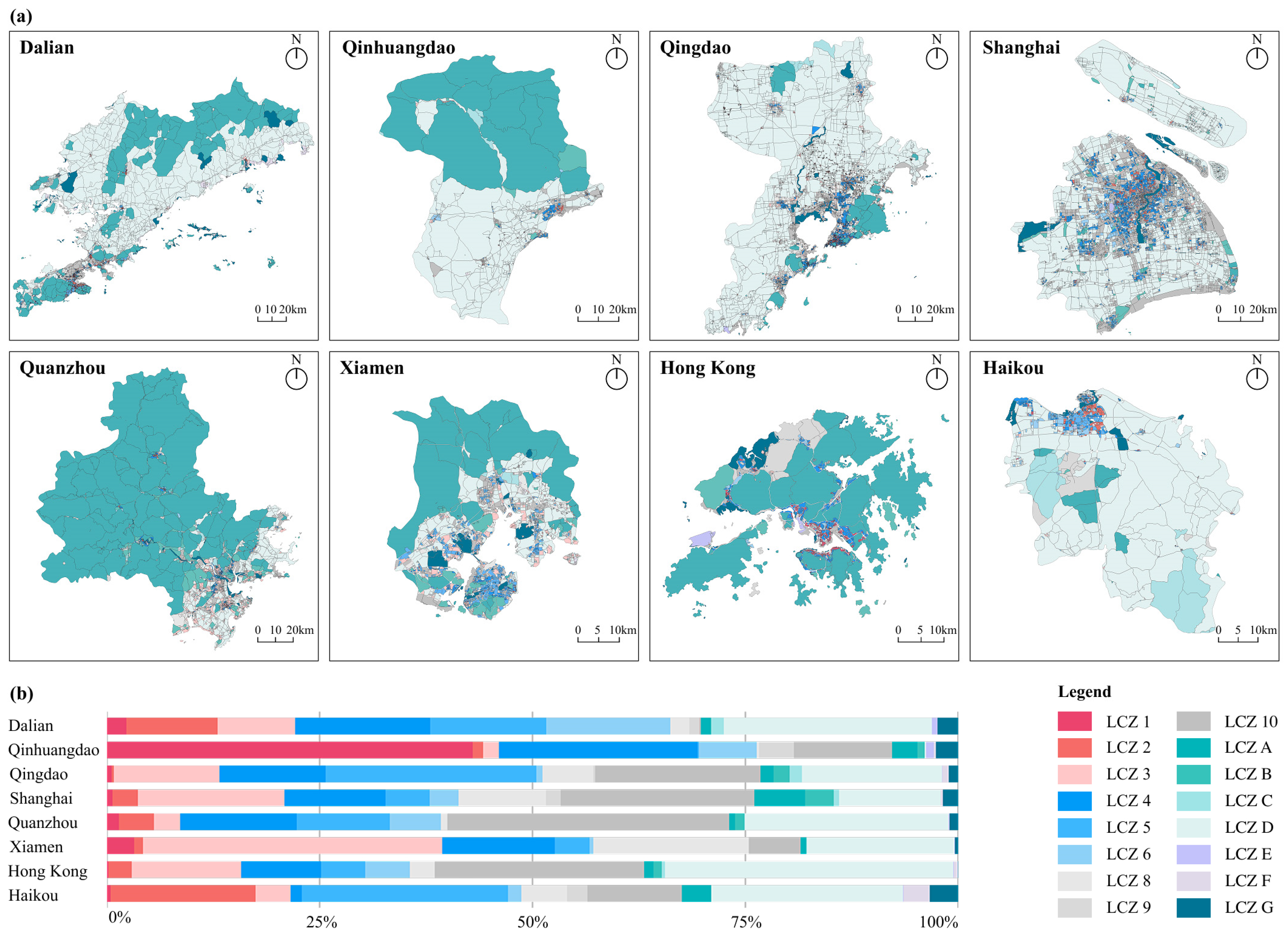
This study focuses on eight representative cities along China’s eastern coast: Dalian, Qinhuangdao, Qingdao, Shanghai, Quanzhou, Xiamen, Hong Kong, and Haikou (Figure 1). These cities cover different climate zones, urban development patterns, and geographical characteristics in China’s coastal regions.
The selected cities are distributed along the Bohai Sea, Yellow Sea, East China Sea, and South China Sea, covering China’s main sea areas. Dalian (38°43′–40°12′ N, 120°58′–123°31′ E) is located at the junction of the Yellow Sea and Bohai Sea, with long winters and short summers. Dalian has over 6 million residents and has experienced rapid urbanization, with temperatures rising 3.45 °C per century [55]. From July to August 2018, the highest temperatures exceeded 30 °C for 8 consecutive days for the first time in history. Qinhuangdao (39°52′–40°32′ N, 119°12′–119°57′ E) is a major port on the Bohai Sea with a temperate monsoon climate. Qinhuangdao, as a part of the Beijing Tianjin Hebei urban agglomeration, has a city warming rate of 0.16 °C per decade [56]. Qingdao (35°35′–37°09′ N, 119°30′–121°00′ E) is located on the Yellow Sea coast in a transition zone from temperate monsoon to subtropical monsoon climate. Shanghai (30°40′–31°53′ N, 120°52′–122°12′ E) is the largest metropolis on the East China Sea coast, with a population exceeding 24 million and an urbanization rate of 88% [57]. The year 2024 was the hottest since Shanghai began keeping records in 1873, with 12 consecutive days of heat waves ≥37 °C in August 2024 [58]. Rapid warming has increased the mortality rate of high temperatures in Shanghai by 13%, with a 19% increase in cardiovascular disease mortality [59,60]. Temperature sensitivity analysis reveals that for every degree above 25 °C, Shanghai experiences a 14.5% increase in daily electricity consumption. Quanzhou and Xiamen (24°23′–25°56′ N, 117°53′–119°05′ E) are located along the Taiwan Strait coast with subtropical monsoon climate. Extreme high temperature and precipitation events in Xiamen have significantly increased since the 1990s, with obvious UHIs. Between 1960 and 2019, UHIs contributed to 38.8% of the local temperature increase [61]. Hong Kong (22°08′–22°35′ N, 113°49′–114°31′ E) is a typical high-density development area in the Pearl River Estuary. Long-term warming trends show that Hong Kong’s warming rate from 1885 to 2024 was 0.14 °C/decade. 2024 set the hottest record in 140 years, with 35 record-breaking high-temperature events throughout the year [62]. Hong Kong’s comprehensive monitoring reveals 1,677 excess deaths across 18 heatwaves between 2014 and 2023 [63]. Haikou (19°57′–20°05′ N, 110°10′–110°23′ E) is located in the South China Sea area of Hainan Island, with tropical coastal city development characteristics. FY-3D satellite data shows that Haikou had the strongest UHI intensity in August, with an average temperature difference of 0.76 °C between the built-up area and the outskirts [64]. Its UHI range evolution rate is at a relatively high level [65]. These cities generally face severe urban heat island challenges, posing threats to resident health, energy consumption, and urban sustainable development. This study uses city blocks as basic analysis units, with detailed block quantities for each city shown in Figure 1.

2.2. Data Sources and Processing

The data used in this study are shown in Table 1: (1) Landsat 8 Collection 2 Level-2 product data, with 30 m spatial resolution, acquisition time from 1 June to 15 August 2023 (summer), used to calculate LST, ALB, and NDVI; (2) Block division data from the Multi-Scale Dense City-Wide (MSDCW) Dataset, providing multi-level block division data for 985 global cities [66], offering standardized spatial analysis units for cross-city comparative analysis; (3) Land use/cover data from the Global Land Cover with Fine Classification System at 10 m (GLC_FCS10) dataset, with 10 m spatial resolution and overall global accuracy of 83.16% [67]; (4) Tree height data from sub-meter resolution canopy height maps [68]; (5) Building data from the 3D Global Building Footprint Product (3D-GloBFP) dataset [69], the first global three-dimensional building footprint dataset; (6) Population density data using 100 m gridded datasets constructed based on China’s seventh population census [70]; (7) Nighttime light data using “The global National Polar-orbiting Partnership Visible Infrared Imaging Radiometer Suite (NPP-VIIRS)-like nighttime light data (Version 2) for 1992–2024” dataset, with 100 m spatial resolution [71]; (8) China coastline data extracted from OpenStreetMap.
This study selected 14 influencing factors, as shown in Table 2, covering five categories: biophysical parameters, building morphology, landscape indicators, geographic location, and social indicators. Albedo (ALB) and Normalized Difference Vegetation Index (NDVI) were calculated through cloud masking and radiometric calibration on the Google Earth Engine (GEE) platform, with ALB calculated using the Liang algorithm [72] and NDVI calculated using the standard band ratio formula (NIR–Red)/(NIR + Red).
Building Density (BD), Building Height (BH), and Sky View Factor (SVF) were calculated based on 3D building data, where BD is the ratio of building footprint area to total block area, and BH is the average height of buildings within blocks. SVF was calculated using a ray-casting algorithm on rasterized building height data. The sampling casts 16 rays from each pixel location within a 10-pixel radius, assuming buildings are opaque obstacles. SVF equals the ratio of unobstructed rays to total rays, ranging from 0 (fully obstructed) to 1 (open sky). Landscape indicators including Aggregation Index (AI), Cohesion Index (COH), Landscape Shape Index (LSI), Shannon Diversity Index (SHDI), and Split Index (SPL) were calculated based on land use/cover data using the landscapemetrics package in RStudio (version: 2024.12.1+563). Tree Height (TH) data was processed to 30 m resolution through the GEE platform. Distance from Sea (DS) was calculated using the nearest neighbor method. Nighttime Light (NTL) data and Population Density (PD) data reflect human activity intensity and population distribution characteristics, respectively. All datasets were standardized and aggregated to the block level using zonal statistics methods, with continuous variables taking average values within blocks and categorical variables taking dominant categories.

3. Methodology

3.1. Overview

This study employed a five-step workflow to explore the driving mechanisms of coastal city UHII (Figure 2). First, based on the GEE platform, multi-source remote sensing data were integrated, and random forest algorithms were used for LCZ classification. Second, Landsat 8 products were used to extract land surface temperature and calculate UHII while integrating 14 influencing factors. Third, descriptive statistical analysis of UHII in eight coastal cities was conducted to reveal urban heat island characteristics of different cities and LCZ types. Fourth, XGBoost models were used to establish nonlinear relationships between influencing factors and UHII, and SHAP methods were used to identify key driving factor importance and marginal effects. Finally, causal inference methods were used to identify causal relationships between important influencing factors and UHII.

3.2. Machine Learning-Based LCZ Classification Method

LCZ classification is fundamental in the study of urban thermal environments. According to a review of the relevant literature, LCZ classification methods mainly include three categories: manual interpretation, automatic classification based on statistical indicators, and machine learning classification. Among them, machine learning-based classification methods are widely used due to their high efficiency and high classification accuracy [73]. Considering that the research area covers multiple coastal cities and the urban forms are complex and diverse, we constructed an LCZ classification method based on the random forest algorithm.
We integrated multi-source remote sensing data for LCZ classification based on the GEE platform. Landsat 8 Collection 2 Level-2 data acquisition time ranged from 1 June to 15 August 2023, with cloud coverage threshold controlled within 20%. All images underwent standardized cloud masking and radiometric calibration, with optical band scaling factors of 0.0000275 and offset of −0.2, and thermal infrared band scaling factors of 0.00341802 and offset of 149.0.
This study employed random forest classifiers containing 200 decision trees for LCZ classification. Classification features included 6 spectral bands (blue, green, red, near-infrared, shortwave infrared 1, shortwave infrared 2), 5 spectral indices (NDVI, NDBI, MNDWI, LSWI, NDSVI), and 3 topographic factors (elevation, slope, aspect), totaling 14 input features.
Sample point collection used random sampling methods with manual annotation using high-resolution remote sensing images. Sufficient samples (>20) were selected for each LCZ type, ensuring samples were spatially evenly distributed and covered typical urban morphologies of each city. Data division involved a random partitioning strategy, dividing sample data into training and testing sets at an 8:2 ratio. Training sets were used for model training and parameter optimization, while testing sets were used for model performance evaluation and accuracy verification. Classification accuracy evaluation used confusion matrix analysis methods, calculating overall accuracy and kappa coefficients. LCZ classification accuracy results for each city are detailed in Table 3.

3.3. LST and UHII Calculation

This study used Landsat 8 Collection 2 Level-2 land surface temperature products for LST acquisition based on the GEE platform. We selected summer images from 1 June to 15 August 2023, with cloud coverage threshold set within 20% to ensure data quality. During data preprocessing, cloud masking was first performed based on QA_PIXEL quality assessment bands. Cloud and cloud shadow pixels were identified through bit operations, where bits 3 and 4 correspond to cloud and cloud shadow identifiers, respectively, constructing mask conditions to remove cloud-affected pixels. Radiometric calibration was then performed, applying official scaling factors and offsets to convert Digital Number (DN) values to physical temperature values [74]:
T K e l v i n = D N × 0.00341802 + 149.0
T C e l s i u s = T K e l v i n 273.153  
where T K e l v i n is temperature in Kelvin and T C e l s i u s is temperature in Celsius. Mean compositing methods were applied to all images passing quality control during the study period, generating summer land surface temperature maps for 8 cities with 30 m spatial resolution in Celsius (°C).
The UHII designed in this study is surface urban heat island intensity, measured in degrees Celsius (°C). According to Deng et al. [17], LCZ 9 (sparsely built), LCZ B (scattered trees), and LCZ D (low plants) were selected as non-urban reference areas, representing relatively natural surface conditions. The UHII calculation formula is as follows:
U H I I = L S T L C Z X L S T L C Z 9 - + L S T L C Z B - + L S T L C Z D - 3  
where UHII is urban heat island intensity; L S T L C Z X represents the average land surface temperature of each LCZ type; and L S T L C Z 9 - , L S T L C Z B - , and L S T L C Z D - represent average land surface temperatures of LCZ 9, LCZ B, and LCZ D, respectively.

3.4. XGBoost–SHAP Machine Learning Model

XGBoost is an ensemble learning model based on gradient boosted decision trees. XGBoost uses a boosting framework, iteratively training multiple decision trees to gradually correct errors from previous rounds to enhance overall prediction performance. Compared to traditional gradient boosted decision trees models, XGBoost integrates weighted loss optimization, regularization techniques, and parallel computing, showing excellent performance in computational efficiency, generalization ability, and interpretability [75].
This study used 5-fold cross-validation to ensure model stability and generalization ability, with random search iterating 50 times to find optimal parameter combinations. To ensure experimental reproducibility, the random seed was set to 42. Data was divided into training and testing sets at an 8:2 ratio, using coefficient of determination (R2) and Root Mean Square Error (RMSE) as model evaluation metrics.
The black-box characteristics of machine learning models make them lack transparency and interpretability. SHAP models provide effective pathways for explaining model decision processes. SHAP models are interpretability algorithms based on cooperative game theory, with core principles of calculating each feature’s marginal contribution to model predictions, decomposing overall prediction results into sums of individual feature contributions, thereby quantifying each feature’s impact on model predictions. SHAP value calculation is based on Shapley value theory, ensuring consistency and fairness of explanation results by considering all possible feature combinations [76]. The SHAP value calculation formula for feature “i” is as follows:
ϕ i = S N i   S !   N S 1 ! N ! f x S i f x S
where ϕ i represents the SHAP value of feature i for UHII; N is the set of all features; S is a feature subset not containing feature i ; f x ( S ) is the model prediction value using feature subset S ; f x ( S { i } ) is the prediction value including feature i ; and the weight term ensures fair consideration of all feature combinations.
This study used 14 multidimensional urban factors as independent variables and UHII values as dependent variables, utilizing XGBoost algorithms in Python 3.11 to construct prediction models. TreeExplainer was used to calculate the SHAP values of optimal models on test sets, employing beeswarm plots to show relationships between feature values and SHAP values and constructing partial dependence plots to analyze the marginal effects of the top 4 important features, revealing nonlinear response patterns of influencing factors on UHII.

3.5. Causal Inference

Traditional machine learning methods can only identify statistical associations and cannot reveal causal relationships between variables. This study adopted structural causal model frameworks, exploring the causal effects of key influencing factors on UHII based on SHAP analysis results.

3.5.1. Causal Variable Selection and DAG Construction

Based on SHAP importance rankings, the top three influencing factors for each city were selected as candidate causal variables. Directed Acyclic Graphs (DAGs) were constructed to represent causal relationships between variables, employing do-calculus theory to quantify causal influences on UHII. Causal graph construction followed urban climatology theory-based determination of prior causal relationships. For instance, distance to shoreline affects population density through historical settlement patterns, population density influences night-time lights through economic activities, and all variables have direct or indirect pathways to UHII. The causal relationships were encoded in DAG structures specific to each city’s urban morphology and development patterns.

3.5.2. Confounder Identification and Validation

Confounders were systematically identified through a three-step process. First, backdoor path analysis identified variables blocking all backdoor paths between treatment and outcome using the backdoor criterion. A variable C is a confounder if there exists an unblocked backdoor path from treatment T to outcome Y through C, and conditioning on C blocks this path. Second, statistical validation was performed using conditional independence tests. Variables were confirmed as confounders when:
P T | T , C P Y | T   a n d   P T | C P T
where Y is UHII, T is treatment variable, and C represents potential confounders.
Third, domain knowledge from urban climatology literature guided identification of variables simultaneously affecting both treatment and outcome. For example, elevation influences both vegetation distribution and temperature through atmospheric pressure and precipitation patterns. All identified confounders were verified using d-separation algorithms to ensure they blocked backdoor paths.

3.5.3. Causal Effect Estimation

The causal identification strategy relied on three key assumptions: (1) Conditional exchangeability (unconfoundedness)—no unmeasured confounding given observed covariates; (2) Positivity—all units have non-zero probability of receiving each treatment level given confounders; (3) Consistency—observed outcomes equal potential outcomes under received treatment.
The Average Treatment Effect (ATE) was estimated using backdoor adjustment based on do-calculus:
A T E = E Y d o X = 1 E Y d o X = 0
where E ·   represents   the   mean ,   Y represents UHII, X represents intervention variables, and d o ( · ) represents intervention operations. For continuous variables, marginal structural models were used to estimate causal effects under different intervention levels. To handle selection bias and confounding effects in observational data, inverse probability weighting methods were employed:
A T E I P W = E Y × T e X Y × 1 T 1 e X
where T is the binarized intervention variable, and e ( X ) is the propensity score estimated through logistic regression, reflecting the probability of individuals receiving intervention.
Following ATE estimation, we calculated elasticity coefficients to assess policy sensitivity:
ε = A T E × X Y
where ε is the elasticity coefficient, ATE represents the average treatment effect in original units (°C per unit change in treatment), and X , Y are mean values of treatment and outcome variables, respectively. Although standardized data were used during estimation for numerical stability, the ATE values are expressed in original units. The elasticity coefficient thus represents the percentage change in UHII per 1% change from the mean value of each factor.

3.5.4. Robustness Tests and Sensitivity Analysis

To ensure result robustness, comprehensive refutation tests were conducted. Placebo treatment tests replaced actual treatment with randomly permuted values while maintaining statistical properties:
β ^ p l a c e b o = E Y | T p e r m u t e d , C E Y | C
where β ^ p l a c e b o is the estimated effect under placebo treatment, Y is UHII, T p e r m u t e d is the randomly permuted treatment variable, C represents confounders, and E[·] denotes expectation. Valid causal estimates should yield null effects under placebo treatment (p > 0.05).
Random common cause tests added randomly generated variables as pseudo-confounders to test estimate stability. Robust estimates should remain stable when controlling for irrelevant variables. Data subset validation re-estimated causal effects on bootstrap samples (n = 100) to assess sensitivity to sampling variation.
Sensitivity analysis evaluated potential impacts of unobserved confounding variables. The analysis quantified the minimum strength of unmeasured confounding needed to nullify observed effects, acknowledging that factors such as microscale urban morphology or anthropogenic heat emissions may influence results.

4. Results

4.1. Block-LCZ Classification Results

The 8 coastal cities collectively contain 16 LCZ types, with each city demonstrating relatively diverse LCZ type compositions (Figure 3). While high-density built-up areas (LCZ 1-LCZ 6) are concentrated primarily in urban core areas, medium–low-density built types extend outward in gradients. In contrast, natural cover types are distributed widely in urban peripheral zones. Although water bodies (LCZ G) maintain certain proportional distributions across all cities, their spatial patterns vary according to specific geographical conditions and coastline morphology.
The dominant LCZ types across cities exhibit distinct regional characteristics. Hong Kong is dominated by LCZ 1 blocks (compact high-rise), accounting for 43%, which reflects its high-density vertical development pattern. Conversely, Qingdao is characterized by LCZ 3 blocks (compact low-rise), representing traditional low-rise high-density building patterns. Whereas these cities show single-type dominance, Shanghai, Quanzhou, and Qinhuangdao are all dominated by LCZ 10 blocks (heavy industry), indicating their industrial development orientation. From the overall block statistics, LCZ D blocks (low plants) achieve the widest distribution at 19.2%, while LCZ E blocks (bare rock or paved) account for only 0.1%, suggesting relatively high urbanization levels coupled with adequate ecological coverage in the study areas.

4.2. Spatial Distribution of UHIs and Thermal Characteristics of Various LCZ Types

The spatial organization patterns of UHIs demonstrate significant differentiation among cities (Figure 4). Shanghai exhibits a concentrated heat island pattern, with core built-up areas forming large, continuous regions of intense heat islands, consistent with megacity development characteristics. In comparison, Qingdao and Dalian display multi-core, dispersed heat island distributions, with spatially fragmented heat hotspots that correspond to their clustered urban development models. Hong Kong and Quanzhou show heat island distributions influenced by topography, resulting in banded patterns along coastlines and valleys, whereas Qinhuangdao and Haikou feature relatively uniform heat island distributions without distinct local super-high temperature zones.
The cities’ average UHII rankings are as follows: Hong Kong (2.63 °C) > Qingdao (2.48 °C) > Dalian (1.61 °C) > Qinhuangdao (1.42 °C) > Haikou (1.27 °C) > Xiamen (0.62 °C) > Shanghai (−0.14 °C) = Quanzhou (−0.14 °C). Notably, the three northern coastal cities tend to have higher heat island intensities.
Significant differences in UHII are observed across different built-up LCZ block types. Among compact built types, LCZ 1 (compact high-rise), LCZ 2 (compact midrise), and LCZ 3 (compact low-rise) blocks all exhibit strong heat island effects. LCZ 2 blocks show the highest average UHII values in most cities, reaching 7.1 °C in Qingdao and 5.49 °C in Dalian. The average UHII of LCZ 1 blocks is positive in all six cities where this type is present. The average UHII of LCZ 3 blocks shows notable regional differentiation, with the northern cities of Qingdao (5.55 °C) and Qinhuangdao (4.38 °C) significantly higher than the southern cities of Xiamen (1.92 °C) and Shanghai (1.52 °C). The UHII of open built-type LCZ (LCZ4-6) blocks tends to be lower, but with greater variability. Notably, the average UHII of LCZ 6 blocks in Shanghai and Quanzhou is negative, indicating that open-building-layout blocks have cooling effects under certain conditions.
Among natural cover types, LCZ G (water) blocks and LCZ A (dense trees) blocks show negative average UHII values across all cities, reflecting the stable cooling effects of natural elements in urban thermal environments. UHII in LCZ 10 (heavy industry) blocks shows significant regional variation, with the northern cities of Qingdao (5.49 °C) and Dalian (4.59 °C) exhibiting higher values than southern cities, likely due to differences in industrial structures and production intensities. LCZ D (low plants) blocks, dominated by farmland landscapes, generally have average UHII values close to 0 °C in most cities, acting as important urban buffer zones. Overall, the heat island characteristics of coastal city LCZ blocks are influenced by factors such as building density, natural elements, and geographical location. Different LCZ types play varying roles in regulating the urban thermal environment, with clear regional differentiation in their effects.

4.3. Impact of Multidimensional Urban Influencing Factors on UHII in Coastal Cities

4.3.1. Model Performance Evaluation and Validation

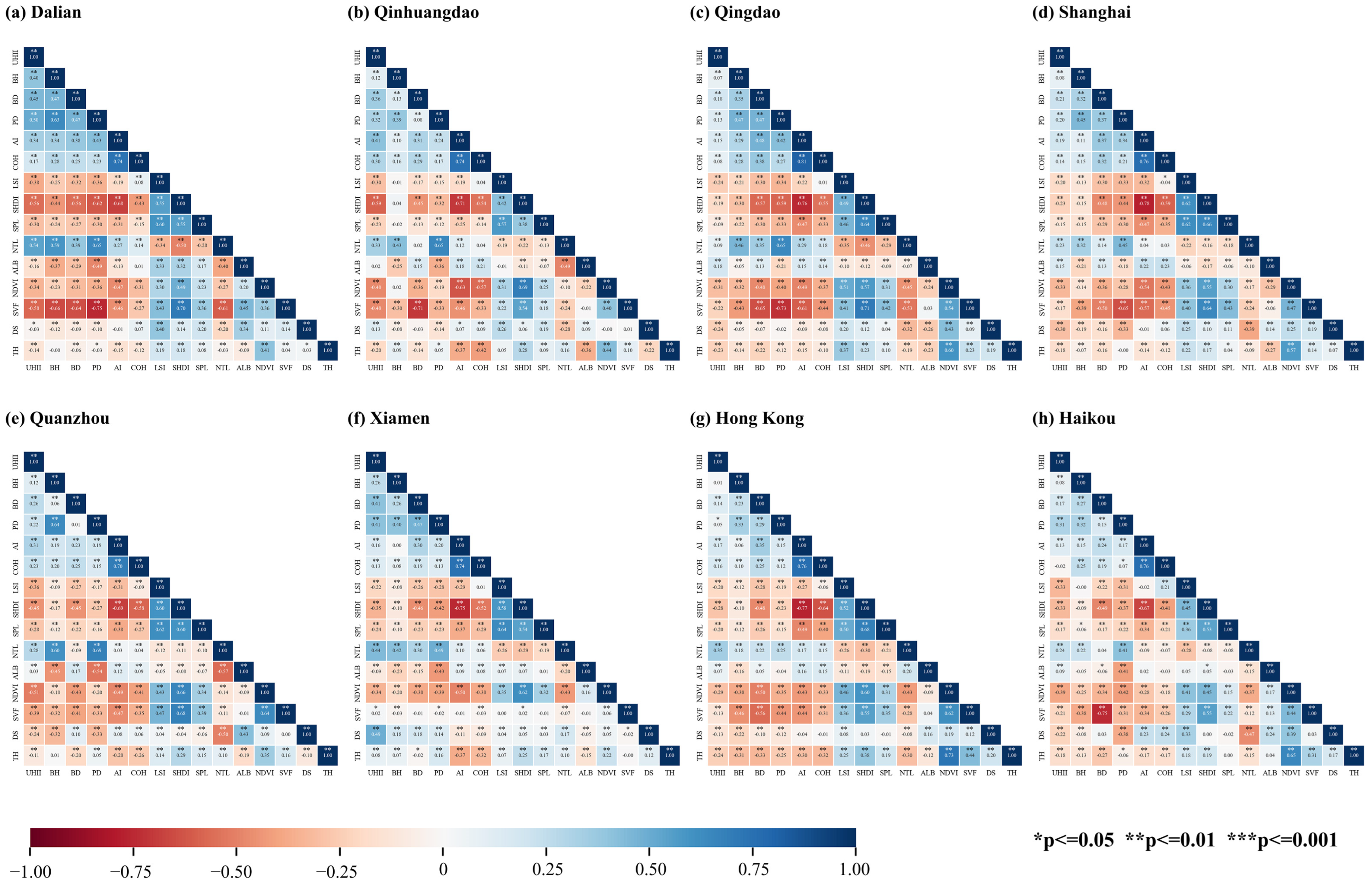
Before establishing the models, we first conducted a correlation analysis of all influencing factors. Figure 5 shows that the correlation coefficients among all influencing factors are <0.8, indicating that there are no significant multicollinearity issues among the factors.
To validate our model selection, we compared XGBoost’s performance against seven alternative algorithms, including baseline linear models (Linear Regression [LR], Ridge Regression [RR], and Lasso Regression), traditional machine learning methods (Decision Tree [DT] and K-Nearest Neighbors [KNN]), and advanced ensemble algorithms (Random Forest [RF] and Light Gradient Boosting Machine [LGBM]) (Figure 6). The results demonstrated clear performance stratification: linear baseline models (LR, RR, and Lasso) showed limited predictive capability (R2 < 0.27), indicating their inability to capture the complex non-linear relationships between urban factors and UHII. Among the advanced methods, ensemble algorithms (XGBoost, RF, LGBM) significantly outperformed single learners, with XGBoost achieving the highest accuracy (R2 = 0.638). This superior performance, combined with XGBoost’s computational efficiency and seamless integration with SHAP for interpretability analysis, validated our methodological choice.
XGBoost’s predictive accuracy showed variation across the eight coastal cities (Table 4). While some cities demonstrated excellent model performance, four cities—Quanzhou (R2 = 0.44), Haikou (R2 = 0.43), Hong Kong (R2 = 0.45), and Xiamen (R2 = 0.48)—showed moderate predictive capability. This performance variation can be primarily attributed to sample size constraints, as machine learning algorithms typically require substantial training datasets for optimal performance. Cities with fewer blocks inherently limit model training capacity, which may explain the observed differences in predictive accuracy. Despite these constraints, our moderate-performing models remain comparable to recent machine learning studies on urban thermal environments (e.g., Chen et al., 2024: R2 = 0.38−0.55 [77]; Wang et al., 2025: R2 = 0.0.457−0.587 [78]; Zuo et al., 2025: R2 = 0.46 [79]).

4.3.2. Factor Importance and SHAP Value Analysis

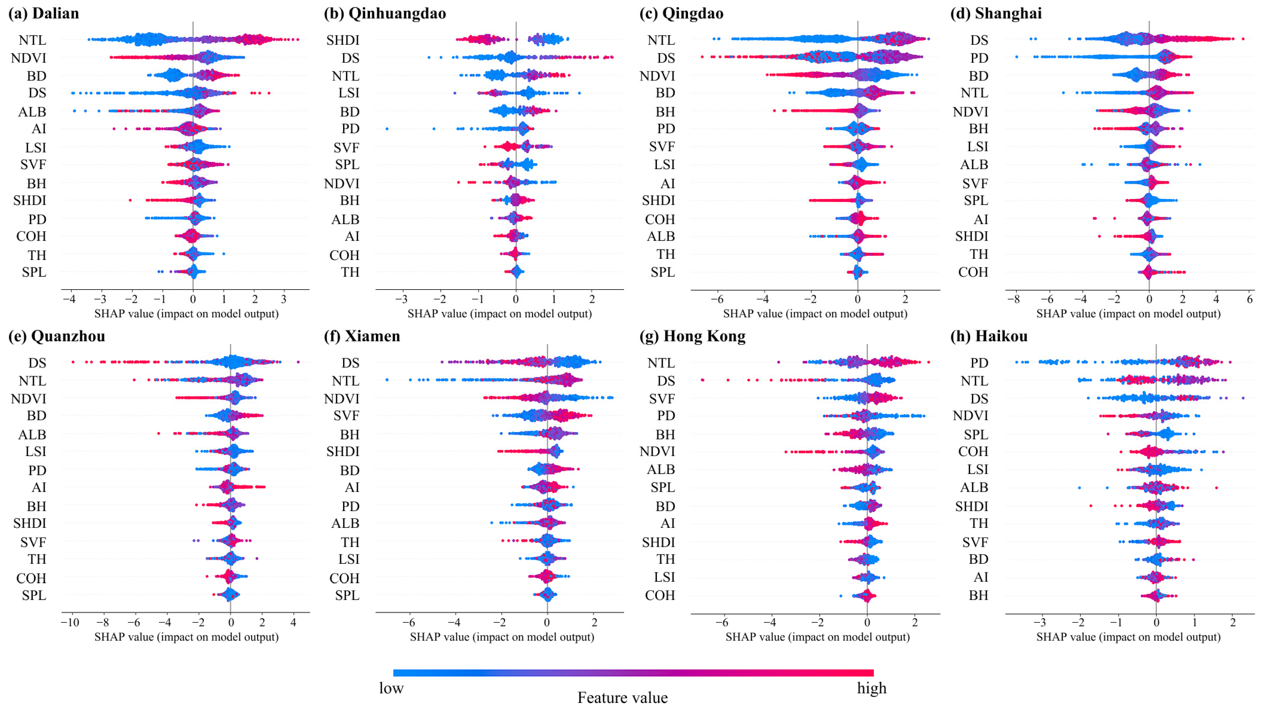
We employed XGBoost–SHAP models to investigate the relationships between 14 influencing factors and UHII. Figure 7 displays the rankings of the contributing factors to UHII and the distribution of SHAP values. Across all eight coastal cities, NTL and DS are the most important factors affecting UHII, ranking first in three cities each and placing in the top four in all cities. This suggests that human activity intensity and geographical factors play dominant roles in shaping the thermal environments of coastal cities. Other significant factors include NDVI, BD, and PD, which rank among the top eight in most cities, while the impacts of COH, TH, and SPL are relatively smaller.
Several influencing factors demonstrate notable city-specific variations. For instance, SHDI ranks first in Qinhuangdao for its influence on UHII, whereas it ranks sixth in Xiamen and tenth in Dalian, Qingdao, and Quanzhou. Similarly, PD shows strong influence in Haikou and Shanghai (ranking 1st and 2nd, respectively) but demonstrates less influence in Dalian. BD exhibits strong impacts on UHII in Dalian, Shanghai, and Quanzhou (ranking in the top four), while its influence decreases significantly in Haikou (12th place). Furthermore, SVF ranks highly in Hong Kong and Xiamen (3rd and 4th) but shows limited impact in Quanzhou and Haikou (11th). SPL has minimal impact on UHII in most cities, ranking last in Dalian, Qingdao, Quanzhou, and Xiamen, with the exception of Haikou, where it ranks 5th.
Concerning the directional impacts on UHII, BD, DS, and ALB consistently show positive effects across all cities, while NDVI, SHDI, LSI, and SPL demonstrate negative effects. The impact directions of other factors vary between cities. NTL, PD, and AI generally produce positive impacts on UHII. Although SVF typically exerts positive effects in most cities, it shows negative impacts in Qinhuangdao, with unclear effects in Dalian and Qingdao. The impacts of COH, TH, and BH differ across cities.

4.3.3. Marginal Effects Analysis

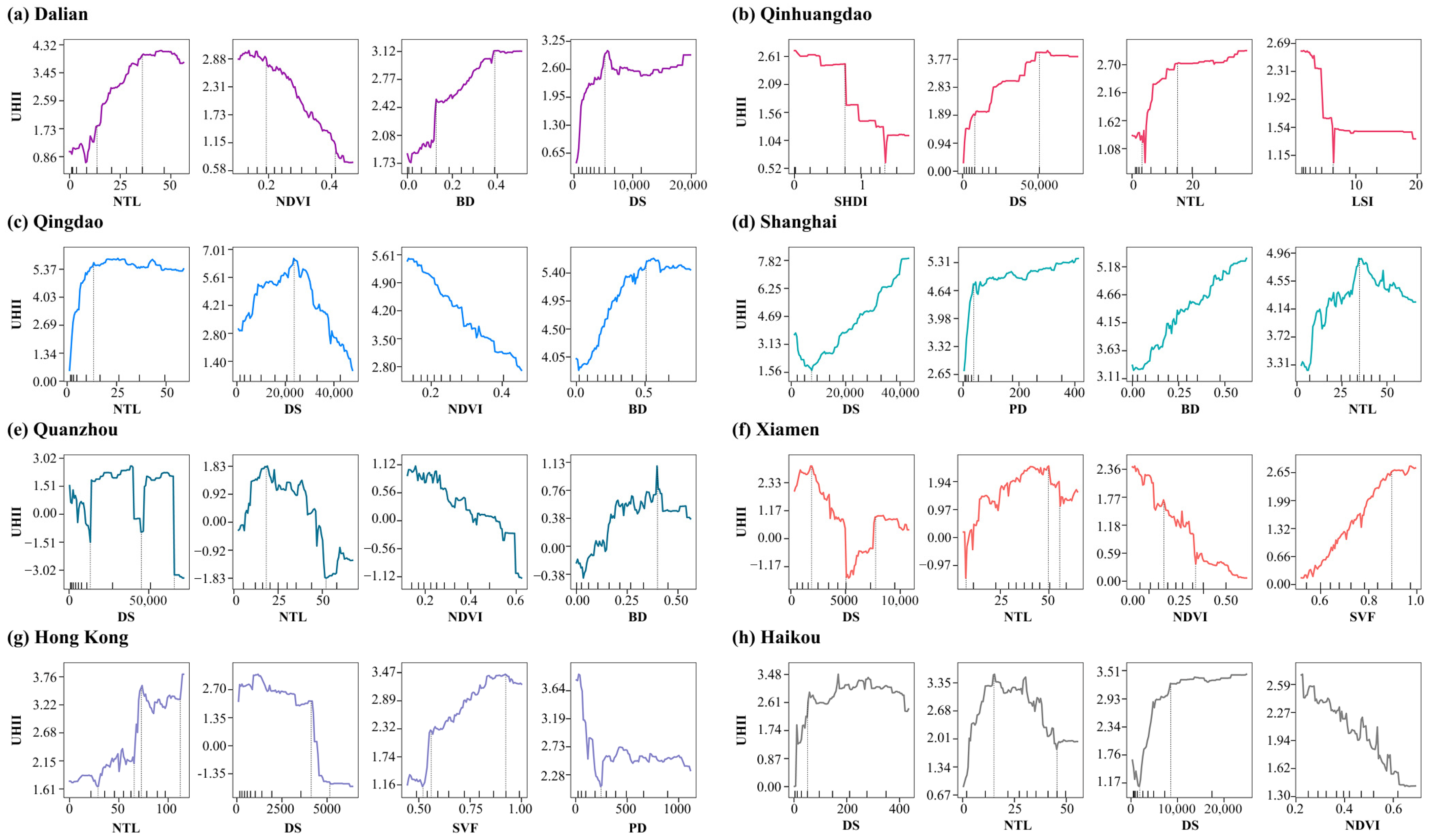
To further investigate the impacts of various influencing factors on UHII, we selected the top four factors with the greatest impact on UHII in each city and analyzed their marginal effects (Figure 8). The influencing factors demonstrate distinct regional patterns. NDVI consistently produces negative impacts across all cities, with UHII decreasing by over 2 °C when NDVI ranges between 0.2 and 0.4 in Dalian, Qingdao, and Xiamen. While most coastal cities exhibit similar hump-shaped NTL patterns, Hong Kong presents a notable exception. Specifically, UHII rises rapidly in the NTL 0–20 interval across most cities—in Qingdao, the warming amplitude exceeds 5.3 °C. Once NTL surpasses 20, UHII values stabilize before declining. Conversely, Hong Kong, characterized by super-high intensity development, displays a stepped ascending curve for NTL.
The DS factor shows considerable regional differences. In Dalian and Qinhuangdao, DS is significantly positively correlated with UHII. The DS trends in Shanghai and Haikou are similar; in Shanghai, when DS < 7450 m, and in Haikou, when DS < 1800 m, there are negative correlations with UHII, which then turn positive. In Qingdao, there is a positive correlation with UHII when DS < 23,700 m, followed by a negative correlation. In Hong Kong, when DS < 4200 m, UHII stabilizes at a high value around 2.7 °C and then declines rapidly, with UHII values stabilizing again when DS > 5000 m. DS in Quanzhou and Xiamen shows complex nonlinear relationships with UHII.
PD in Shanghai and Haikou shows positive correlations with UHII, with strong positive correlations when PD < 43 and PD < 59, respectively. Hong Kong shows opposite results, with strong negative correlations when PD < 246, then gradually stabilizing. Building indicators BD and SVF generally show positive correlations with UHII.

4.4. Causal Inference of Key Influencing Factors on UHII in Coastal Cities

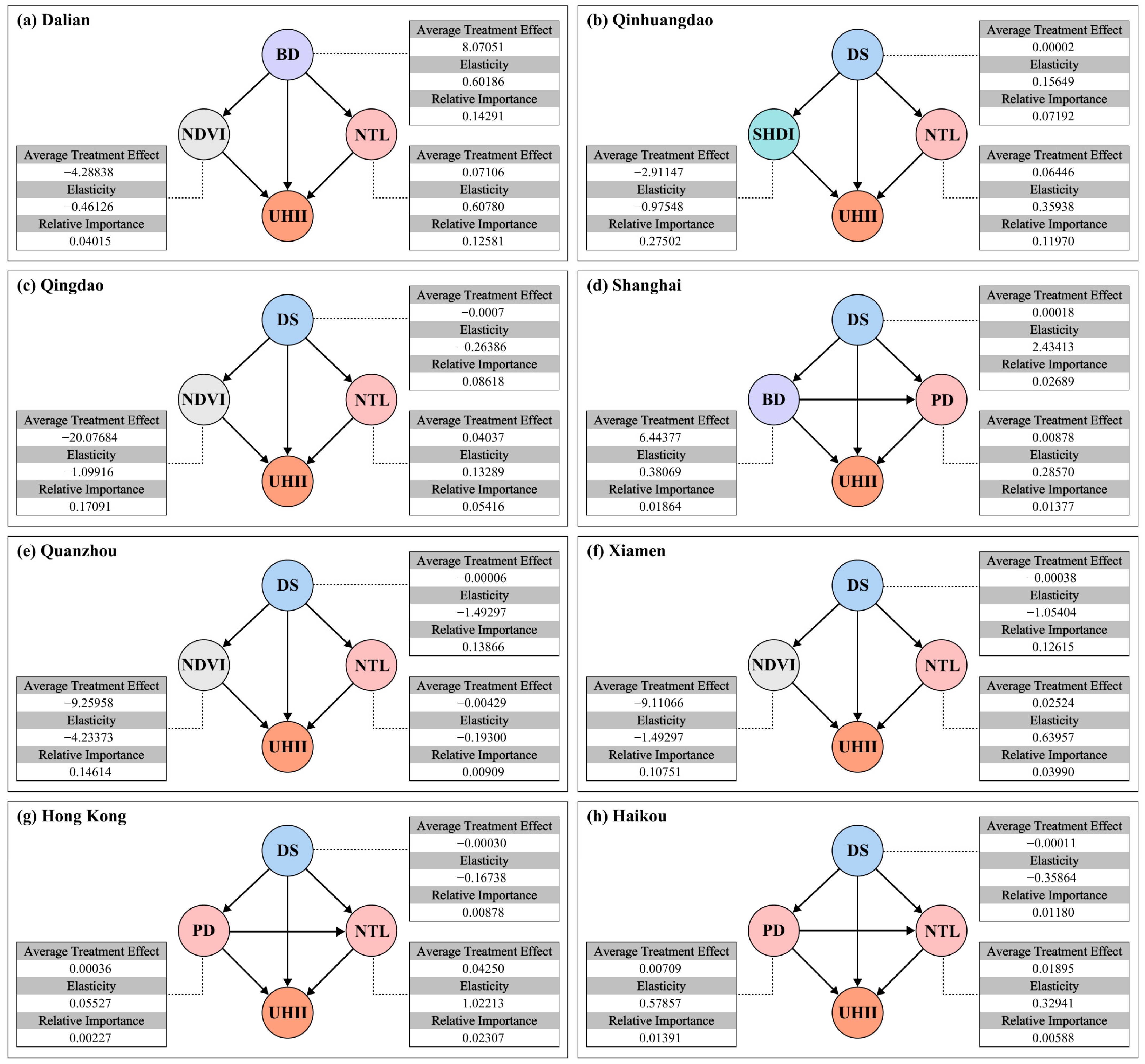
We selected the top three factors based on contribution rankings for each city to construct causal models with UHII (Figure 9). We employed three key indicators: (1) Average Treatment Effect (ATE) quantifying causal impact in original units (°C per unit change); (2) elasticity coefficients for policy sensitivity, calculated as the percentage change in UHII per 1% change from the mean value of each factor—using mean values as reference points ensures stable interpretation for both bounded and unbounded factors (mean values of all factors are presented in Appendix A Table A2); (3) relative importance for proportional contributions within multi-causal systems. All presented causal relationships passed triple refutation tests, except for Hong Kong’s SVF→UHII relationship, which required replacement with PD-related pathways (ranked fourth in contribution). It should be noted that DS’s original ATE unit is °C/m. For ease of interpreting practical significance, we convert it to °C/km (original value × 1000) for reporting.
NDVI demonstrates significant negative causal effects across all involved cities. Quanzhou exhibits the strongest mitigation effect with an elasticity coefficient of −4.23, meaning a 1% increase in NDVI can reduce UHII by 4.23%. Xiamen (Elasticity = −1.49) and Qingdao (Elasticity = −1.10) show secondary mitigation effects, while Dalian has a relatively low elasticity coefficient of −0.46. NDVI has the highest or near-highest relative importance among the three variables in Qingdao (0.17), Quanzhou (0.15), and Xiamen (0.11).
NTL, as a comprehensive indicator reflecting human activity intensity, shows positive causal effects in most cities. Xiamen (0.64) and Dalian (0.61) have the highest elasticity coefficients, indicating that each 1% increase in human activity intensity increases UHII by approximately 0.6%. Qinhuangdao (0.36) and Haikou (0.33) show moderate effects, while Qingdao (0.13) and Hong Kong (0.02) show lower effects. Quanzhou is the only city exhibiting negative effects (Elasticity = −0.19). NTL has the highest relative importance in Dalian (0.13) and Qinhuangdao (0.12).
The causal effects of DS show spatial heterogeneity. Qingdao exhibits the strongest negative effect (ATE = −0.70 °C/km), meaning each kilometer away from the coast reduces UHII by 0.70 °C. Xiamen, Hong Kong, Haikou, and Quanzhou also show negative effects. Conversely, Shanghai shows positive effects (ATE = 0.18 °C/km), where UHII increases by 0.18 °C for each kilometer away from the ocean, and Qinhuangdao shows weaker positive effects (ATE = 0.02 °C/km). DS has the highest relative importance in Quanzhou (0.14) and Xiamen (0.13).
BD shows strong positive causal effects in Dalian and Shanghai. BD elasticity coefficients for UHII in Dalian and Shanghai are 0.60 and 0.38, respectively, with Shanghai BD’s relative importance only 0.02, indicating a relatively small relative contribution of building density in Shanghai’s multi-factor system. SHDI shows strong negative effects in Qinhuangdao (Elasticity = −0.98), with relative importance as high as 0.28, making it the most important heat island mitigation factor in this city. PD shows positive effects in Shanghai (Elasticity = 0.29, Relative importance = 0.01), Haikou (Elasticity = 0.58, Relative importance = 0.01), and Hong Kong (Elasticity = 0.07, Relative importance = 0.002), but with relatively small contributions.

5. Discussion

5.1. Spatial Differentiation Characteristics and Mechanism Analysis of Urban Heat Islands in Coastal Cities

The research results show that UHII in the eight coastal cities exhibit significant spatial differentiation characteristics. This differentiation reflects differences in urban development patterns and geographical environments between cities, and it also reflects the spatial heterogeneity of different LCZ types’ thermal environment contributions.
LCZ 1–3 compact built-up block types show strong heat island effects in most cities. Hong Kong’s topography is dominated by rugged hills, with built-up areas accounting for only 22–25% of the city area [80]. Land scarcity forces cities to adopt ultra-high-density vertical development, with Hong Kong’s LCZ 1 blocks accounting for 43%, with numerous high-rise buildings using “wall-type” layouts forming deep canyons [81]. This layout obstructs natural ventilation, while large amounts of concrete and glass curtain walls absorb solar radiation converted to heat [44].
Notably, LCZ 2 blocks show the highest average UHII values in most cities, consistent with multiple studies including Zhang et al. [82] in Dalian, Zhang et al. [83] in Harbin, and Xiang et al. [84] in Shanghai and Nanjing. This is mainly because mid-rise buildings (3–9 floors) form moderate canyon effects, obstructing ground ventilation while lacking high-rise buildings’ vertical ventilation advantages. As Yelixiati et al. [85] pointed out, dense mid-rise blocks with little green space often produce higher LST. LCZ 4–6 blocks still show strong UHII in most cities, with notable exceptions being Shanghai and Quanzhou LCZ 6 blocks showing slight cooling islands, indicating that cooling potential exists for low-rise building layouts combined with relatively good greening conditions. LCZ G and LCZ A blocks show stable negative UHII values in all cities, reflecting universal regulatory functions of natural elements. In Shanghai and Quanzhou, natural elements’ cooling effects are so prominent that city-wide average UHII values become negative (Shanghai: −0.14 °C)—Shanghai’s extensive water networks (Huangpu River, Suzhou Creek) and Quanzhou’s large mountainous areas provide cooling that exceeds built-up area heating when spatially averaged. However, despite overall negative values, local strongest heat island phenomena still exist at block scales—high-density built-up areas form independent thermal environment systems with intensities far exceeding city-wide levels.
UHII of LCZ 10 blocks shows significant north–south differences, with northern cities like Qingdao and Dalian having significantly higher values than southern cities. This difference may relate to the following factors: firstly, the layout of industrial zones and facilities in the northern region is relatively concentrated; second, heavy industrial structures differ between north and south, with northern cities like Qingdao and Dalian dominated by energy-intensive industries such as steel, petrochemicals, and cement, which generate large amounts of industrial waste heat and anthropogenic heat emissions during production [86].
Inter-city heat island intensity differences also reflect regional climate characteristic influences [81]. Northern coastal cities (Dalian, Qinhuangdao, Qingdao) are located in temperate monsoon climate zones, affected by subtropical high pressure in summer with weaker sea breezes than southern cities, limiting ocean regulatory effects. Southern cities benefit from more stable sea–land wind circulation and year-round vegetation coverage. Overall, spatial differentiation of coastal city heat island intensity results from the comprehensive effects of urban development patterns, land use conditions, geographical environment, and climate conditions.

5.2. Regional Differences in Multidimensional Influencing Factor Mechanisms

This study used XGBoost–SHAP coupled machine learning models to deeply analyze the impact mechanisms of coastal city heat island effects. The research results show that despite significant differences in urban development and geographical environments among the eight coastal cities, they still show some common impact patterns. First, NTL and DS are the most important influencing factors in all cities, highlighting the key positions of human activity intensity and ocean regulatory effects. NDVI generally shows significant negative impacts, with marginal effect curves showing significant cooling effects in the 0.2–0.4 NDVI interval, with UHII decreasing by more than 2 °C in multiple cities. This finding is consistent with research results from Guha et al. [87], Garai et al. [88], and Naga Rajesh et al. [89], all confirming vegetation’s mitigating effects on UHI.
Meanwhile, importance rankings and marginal effects of influencing factors also show significant regional differences between cities. For example, PD performs prominently in Haikou and Shanghai but has weak influence in Dalian, possibly related to urban spatial structure and development patterns. Marginal effect analysis shows that PD impact is particularly significant in lower-density intervals (Haikou < 59, Shanghai < 43), with reduced impact at high densities. This aligns with Oke’s [90] discovery of logarithmic relationships between UHII and population, believing that under conditions of continuous population growth, due to physical limitations of available energy for urban heat island formation, small and medium towns typically experience higher temperature rises than large cities. Hong Kong’s negative PD impact phenomenon deserves attention, possibly because the city’s ultra-high-density development has reached saturation, with spatial variations in population density more reflecting vertical distribution differences rather than horizontal expansion. High-density high-rise building vertical development patterns help mitigate heat island effects to some extent [44], thereby offsetting the warming effects of population concentration.
Complex marginal effect curves shown by DS factors reveal that ocean regulatory effects are far from simple distance–decay relationships but are comprehensively influenced by multiple mechanisms. Qingdao’s DS curve shows obvious staged characteristics, with UHII increasing with distance within 23.7 km, consistent with Guo et al.’s findings of ocean cooling effects weakening with distance [19], thereafter showing declining trends, possibly due to reduced urbanization intensity in inland areas and other local circulation and topographic factors beginning to play dominant roles. Initial negative-then-positive patterns shown by Shanghai and Haikou reveal more complex mechanisms. In near-coastal areas (Shanghai < 7.45 km, Haikou < 1.8 km), UHII decreases with increasing distance, possibly because areas closest to coasts happen to be high-density commercial or port development zones, forming local heat island centers. Research conducted by Wu et al. also found that when coastal areas are dominated by heat source landscapes, water bodies’ cooling capacity changes and weakens [91]. Hong Kong’s unique stepped change pattern is most complex, with UHII stable at high values within 4.2 km DS, rapidly declining in 4.2–5 km intervals, then stabilizing again. This pattern is closely related to Hong Kong’s topographic characteristics, with high-density built-up areas on both sides of Victoria Harbor forming the first high-temperature platform, central ridges blocking sea breezes creating temperature transition zones at 4–5 km, and areas behind mountains forming relatively independent thermal environment systems. Complex fluctuating relationships between DS and UHII in Quanzhou and Xiamen may be caused by multi-scale local circulation systems formed by tortuous coastlines, numerous bays, and islands.
NTL has been confirmed by multiple studies to have significant correlations with UHII [92,93]. This study further analyzed its marginal effects with UHII. NTL shows hump-shaped marginal effect curves in seven cities. UHII rises sharply in low-intensity NTL intervals, with growth slowing or even declining beyond thresholds. This saturation effect may stem from multiple mechanisms: high-intensity development areas typically have more complete infrastructure, intensive development patterns improve energy utilization efficiency, while stricter environmental management measures limit heat emissions. Hong Kong’s unique stepped ascending pattern reflects the predicament of cities with extreme land scarcity and ultra-high-intensity development.
These regional differences in influencing factor mechanisms reflect complex adaptive characteristics of coastal city thermal environment systems. Each city forms unique thermal environment regulatory mechanisms under influences of specific geographical environments, climate conditions, and development patterns.

5.3. UHI Mitigation Strategies Based on Causal Inference

This study provides quantitative insights for coastal city heat island mitigation through causal inference. Based on differences in elasticity coefficients and relative importance observed in our analysis, each city could formulate targeted measures according to dominant driving factors. These findings should be interpreted considering the inherent uncertainties in remote sensing data and urban system complexity.
High NDVI elasticity coefficients in Quanzhou, Xiamen, and Qingdao suggest these cities could prioritize greening optimization as a primary strategy. Quanzhou shows the strongest vegetation cooling effect (ATE = −9.24, elasticity = −4.23), indicating each 1% increase in NDVI is associated with an approximately 4.23% reduction in UHII. Xiamen (ATE = −9.11 °C, elasticity = −1.49) and Qingdao (ATE = −20.07 °C, elasticity = −1.10) also show strong vegetation mitigation potential, with each 1% increase in NDVI associated with 1.49% and 1.10% UHII reductions, respectively. Such cities could expand green space areas and optimize vegetation spatial configurations to maximize cooling effects [94]. Potential measures include increasing road greening and park construction [42] and implementing vertical greening and rooftop gardens [24,95]. In contrast, Dalian’s low NDVI elasticity coefficient (−0.46) and extremely low relative importance (0.04) suggest that relying on vegetation for heat island mitigation may be less efficient; this city might allocate more resources to other measures. Relative importance analysis shows Dalian’s BD (0.14) and NTL (0.13) combined contribute over 25%, suggesting building density optimization and human activity intensity management could be more effective focus areas. Possible measures include setting floor area ratio limits and increasing building spacing to improve ventilation conditions, and promoting energy-efficient buildings to reduce air conditioning waste heat and other multi-level comprehensive controls. This elasticity coefficient-based approach could help to avoid inefficient resource allocation.
Different cities could formulate targeted spatial management strategies based on the differences in DS and UHII relationships identified in our analysis. Cities like Qingdao, Xiamen, Hong Kong, Haikou, and Quanzhou showing negative effects appear to have higher heat island intensities in near-coastal areas; optimization of coastal zone development patterns could be beneficial for these cities. By reducing construction intensity in coastal commercial and port areas, increasing coastal green coverage, and avoiding dense “wall-type” building layouts, they may effectively mitigate high-temperature problems in near-coastal areas. In contrast, positive effects in cities like Shanghai and Qinhuangdao highlight the potential importance of ocean cooling functions; such areas could consider controlling building heights in coastal zones and establishing green ventilation corridors extending from coasts to inland areas [19], utilizing the ocean’s natural regulatory advantages. Additionally, Qinhuangdao’s strong negative SHDI effect (elasticity = −0.98, relative importance = 0.275) suggests that each 1% increase in SHDI correlates with a 0.98% UHII reduction. Recommendations include transforming single-function zones into mixed-function zones and increasing land use type diversity to achieve heat island mitigation.
This section’s contribution lies in identifying driving factors and their effect strengths through causal inference, providing a quantifiable and comparable framework for urban heat island management. While these relationships show statistical significance in our analysis, actual implementation effectiveness would depend on local conditions and should be validated through field studies. Although based on Chinese coastal city data, the causal inference framework itself may have broader applicability and could provide methodological reference for other regions with appropriate adaptations. Future implementation of these strategies requires comprehensive evaluation combining economic costs, technical feasibility, and social acceptability.

5.4. Limitations

However, this study also has some limitations. First, this study uses Landsat 8 data, but its spatial resolution may not capture finer-scale urban thermal environment variations, particularly microclimatic differences within high-density built-up areas. Second, although this study applied strict cloud coverage thresholds for data screening and used temporal window compositing to reduce cloud effects, slight cloud contamination may still exist in some coastal areas, affecting the accuracy of land surface temperature retrieval. Moreover, the inconsistent temporal resolution of multi-source data may introduce bias to the analysis. Third, although this study selected eight representative coastal cities covering China’s major sea areas and different climate zones, there are considerable differences in urban development patterns and geographical environments across China’s coastal regions, and the applicability of research findings to other coastal cities still requires further validation. Fourth, model performance varied across cities. The random train/test split may not fully account for spatial autocorrelation in urban climate data, potentially overestimating model accuracy. Insufficient sample sizes in some cities may also affect the reliability of model interpretations. Future research could employ higher-precision data and expand the sample of cities to further deepen understanding of the driving mechanisms of urban heat island effects in coastal cities, providing scientific support for formulating more precise and effective thermal environment management strategies.

6. Conclusions

UHI research mainly focuses on inland cities, lacking multi-city systematic comparative studies of driving mechanisms in coastal cities under sea-land interactions. Therefore, this study selected eight typical Chinese coastal cities to explore how multidimensional urban factors influence UHII. We constructed block-LCZ spatial analysis units, retrieved LST from remote sensing data to calculate UHII, and analyzed thermal characteristics across cities and LCZ types. Using XGBoost–SHAP models, we examined the contributions and nonlinear impact mechanisms of 14 urban factors on UHII, then identified causal relationships through causal inference methods. The findings reveal the following:
(1)
Significant spatial differentiation of UHII exists among coastal cities, with Hong Kong exhibiting the highest average UHII (2.63 °C) and northern coastal cities generally showing higher values than southern cities. At the LCZ scale, compact building blocks (LCZ 1–3) consistently demonstrate stronger heat island effects than open building blocks (LCZ 4–6), with LCZ 2 showing the most intense heat island effect, while LCZ G and LCZ A blocks provide stable cooling effects across all cities.
(2)
Machine learning models identify distinct nonlinear response patterns of urban factors to UHII. NTL and DS emerge as universally important factors across all cities, while NDVI consistently shows strong negative impacts with optimal cooling effects in the 0.2–0.4 interval. However, factor importance varies significantly between cities—PD ranks in the top two factors in Haikou and Shanghai but shows weak influence in Dalian, while SVF demonstrates high contribution in Hong Kong but limited roles elsewhere.
(3)
Causal inference quantifies city-specific causal relationships between key factors and UHII, enabling differentiated mitigation strategies. Cities with high NDVI elasticity coefficients (Quanzhou and Xiamen) should prioritize vegetation optimization, while Dalian requires focus on building layout optimization given the strong causal effects of building density. The DS causal effects show regional differentiation—negative effects in Qingdao, Xiamen, Hong Kong, Haikou, and Quanzhou suggest potential for enhancing ocean cooling through controlled coastal development, while positive effects in Shanghai and Qinhuangdao indicate the need to protect sea–land ventilation corridors.
While this study focuses on Chinese coastal cities, the block-LCZ analytical framework and causal inference methodology are transferable to other global coastal regions with available remote sensing and urban morphology data. The identified cooling effects of water bodies and vegetation, as well as LCZ-specific thermal patterns, likely apply broadly, though the specific magnitudes and causal relationships may vary with local climate conditions, urban forms, and sea–land interaction intensities.

Author Contributions

Conceptualization, K.L. and H.W.; methodology, K.L. and H.W.; software, H.W.; validation, H.W.; formal analysis, K.L.; investigation, K.L.; resources, K.L.; data curation, H.W.; writing—original draft preparation, K.L.; writing—review and editing, H.W.; visualization, K.L.; supervision, H.W.; project administration, K.L. and H.W.; funding acquisition, H.W. All authors have read and agreed to the published version of the manuscript.

Funding

This work was supported by Hebei Natural Science Foundation [grant number D2025204001]; Science and Technology Project of Hebei Education Department [grant number QN2025433].

Data Availability Statement

The data will be made available upon request.

Conflicts of Interest

The authors declare that they have no known competing financial interests or personal relationships that could have appeared to influence the work reported in this paper.

Abbreviations

The following abbreviations are used in this manuscript:
AIAggregation Index
ALBAlbedo
ATEAverage Treatment Effect
BDBuilding Density
BHBuilding Height
COHPatch Cohesion Index
DSDistance from Sea
GEEGoogle Earth Engine
LCZLocal Climate Zone
LSILandscape Shape Index
LSTLand Surface Temperature
LSWILand Surface Water Index
MNDWIModified Normalized Difference Water Index
NDBINormalized Difference Built-up Index
NDSVINormalized Difference Soil Vegetation Index
NDVINormalized Difference Vegetation Index
NTLNighttime Light
PDPopulation Density
SHAPShapley Additive Explanations
SHDIShannon’s Diversity Index
SPLSplit Index
SVFSky View Factor

Appendix A

Table A1. Detailed data for causal inference.
CityTreatmentOutcomeATEElasticityRelative ImportancePlaceboRandom CauseSubsample
DalianBDUHII8.070510.601860.14291 −0.010308.07009 8.12895
NDVIUHII−4.28838 −0.461260.04015−0.01191 −4.28818−4.28994
NTLUHII0.07106 0.607800.12581 −0.00008 0.07106 0.07123
QinhuangdaoDSUHII0.000020.15649 0.07192 0.00000 0.000020.00002
SHDIUHII−2.91147−0.97548 0.27502 −0.02546−2.91131−2.91735
NTLUHII0.06446 0.35938 0.11970 −0.00103 0.06445 0.06478
QingdaoDSUHII−0.00007 −0.26386 0.08618 −0.00000 −0.00007 −0.00007
NDVIUHII−20.07684 −1.09916 0.17091 0.01088 −20.07696 −20.07575
NTLUHII0.04037 0.13289 0.05416 −0.00024 0.04037 0.04032
ShanghaiDSUHII0.00018 0.88967 0.02689 0.00000 0.00018 0.00018
BDUHII6.44377 0.38069 0.01864 −0.00139 6.44378 6.48544
PDUHII0.00878 0.28570 0.01377 −0.00003 0.00878 0.00883
QuanzhouDSUHII−0.00006−1.49297 0.13866 0.00000 −0.00006 −0.00006
NDVIUHII−9.25958 −4.23373 0.14614 −0.02449 −9.25741 −9.23648
NTLUHII−0.00429 −0.19300 0.00909 0.00075 −0.00429 −0.00452
XiamenDSUHII−0.00038 −1.05404 0.12615 0.00000 −0.00038 −0.00038
NDVIUHII−9.11066 −1.87421 0.10751 0.09011 −9.10853 −9.12213
NTLUHII0.02524 0.63957 0.03990 0.00022 0.02524 0.02546
Hong KongDSUHII−0.00030 −0.16738 0.00878 0.00000 −0.00030 −0.00029
PDUHII0.00036 0.05527 0.00227 0.00001 0.00036 0.00036
NTLUHII0.04250 1.02213 0.02307 −0.00042 0.04251 0.04232
HaikouDSUHII−0.00011 −0.35864 0.01180 −0.00000 −0.00011 −0.00011
PDUHII0.00709 0.57857 0.01391 −0.00004 0.00709 0.00709
NTLUHII0.01895 0.32941 0.00588 0.00027 0.01895 0.01930
Table A2. The mean value of UHII influencing factors in 8 cities.
AIALBBDBHCOHDSLSINDVINTLPDSHDISPLSVFTH
Dalian90.7110.1380.17814.54095.5915874.9937.0420.25620.367119.7710.7814.4220.7920.475
Qinhuangdao89.2110.1550.1277.88496.90517076.4057.5330.22211.80553.6640.7143.9480.8670.625
Qingdao90.7110.1530.32710.51096.80218632.5243.5110.25515.18862.8750.4902.4230.7080.295
Shanghai80.4990.1350.22919.84293.06219158.2296.1320.48133.409125.7461.0344.9100.7470.622
Quanzhou86.5130.1740.20914.99095.59616752.6706.4140.29228.39495.7640.7993.7460.7790.642
Xiamen85.0190.1780.22616.83793.8554226.5374.0380.31337.636135.8820.7913.1560.7440.622
Hong Kong87.8100.1970.67728.18894.9891485.7783.0860.26463.443405.5350.5542.0920.7241.115
Haikou80.1460.1470.1378.79991.6655855.2696.3220.42129.924140.0990.9874.1660.8521.390

References

  1. United Nations Department of Economic and Social Affairs. World Urbanization Prospects 2018: Highlights; United Nations: New York, NY, USA, 2019. [Google Scholar]
  2. Wong, L.P.; Alias, H.; Aghamohammadi, N.; Aghazadeh, S.; Nik Sulaiman, N.M. Urban Heat Island Experience, Control Measures and Health Impact: A Survey among Working Community in the City of Kuala Lumpur. Sustain. Cities Soc. 2017, 35, 660–668. [Google Scholar] [CrossRef]
  3. Li, X.; Zhou, Y.; Yu, S.; Jia, G.; Li, H.; Li, W. Urban Heat Island Impacts on Building Energy Consumption: A Review of Approaches and Findings. Energy 2019, 174, 407–419. [Google Scholar] [CrossRef]
  4. Santamouris, M. Recent Progress on Urban Overheating and Heat Island Research. Integrated Assessment of the Energy, Environmental, Vulnerability and Health Impact. Synergies with the Global Climate Change. Energy Build. 2020, 207, 109482. [Google Scholar] [CrossRef]
  5. Andrés-Anaya, P.; Sánchez-Aparicio, M.; Del Pozo, S.; Lagüela, S. Correlation of Land Surface Temperature with IR Albedo for the Analysis of Urban Heat Island. In Proceedings of the 16th International Workshop on Advanced Infrared Technology & Applications, Online, 26–28 October 2021; MDPI: Basel, Switzerland, 2021; p. 9. [Google Scholar]
  6. Cai, Z.; Han, G.; Chen, M. Do Water Bodies Play an Important Role in the Relationship between Urban Form and Land Surface Temperature? Sustain. Cities Soc. 2018, 39, 487–498. [Google Scholar] [CrossRef]
  7. Guo, J.; Han, G.; Xie, Y.; Cai, Z.; Zhao, Y. Exploring the Relationships between Urban Spatial Form Factors and Land Surface Temperature in Mountainous Area: A Case Study in Chongqing City, China. Sustain. Cities Soc. 2020, 61, 102286. [Google Scholar] [CrossRef]
  8. Li, H.; Li, Y.; Wang, T.; Wang, Z.; Gao, M.; Shen, H. Quantifying 3D Building Form Effects on Urban Land Surface Temperature and Modeling Seasonal Correlation Patterns. Build. Environ. 2021, 204, 108132. [Google Scholar] [CrossRef]
  9. Sun, F.; Liu, M.; Wang, Y.; Wang, H.; Che, Y. The Effects of 3D Architectural Patterns on the Urban Surface Temperature at a Neighborhood Scale: Relative Contributions and Marginal Effects. J. Clean. Prod. 2020, 258, 120706. [Google Scholar] [CrossRef]
  10. Wang, Z.; Zhou, R.; Yu, Y. The Impact of Urban Morphology on Land Surface Temperature under Seasonal and Diurnal Variations: Marginal and Interaction Effects. Build. Environ. 2025, 272, 112673. [Google Scholar] [CrossRef]
  11. Zhou, Y.; Zhang, G.; Jiang, L.; Chen, X.; Xie, T.; Wei, Y.; Xu, L.; Pan, Z.; An, P.; Lun, F. Mapping Local Climate Zones and Their Associated Heat Risk Issues in Beijing: Based on Open Data. Sustain. Cities Soc. 2021, 74, 103174. [Google Scholar] [CrossRef]
  12. Hu, Y.; Dai, Z.; Guldmann, J.-M. Modeling the Impact of 2D/3D Urban Indicators on the Urban Heat Island over Different Seasons: A Boosted Regression Tree Approach. J. Environ. Manag. 2020, 266, 110424. [Google Scholar] [CrossRef]
  13. Kim, M.; Lee, K.; Cho, G.-H. Temporal and Spatial Variability of Urban Heat Island by Geographical Location: A Case Study of Ulsan, Korea. Build. Environ. 2017, 126, 471–482. [Google Scholar] [CrossRef]
  14. Liu, H.; Weng, Q. Seasonal Variations in the Relationship between Landscape Pattern and Land Surface Temperature in Indianapolis, USA. Environ. Monit. Assess. 2008, 144, 199–219. [Google Scholar] [CrossRef]
  15. Feng, R.; Wang, F.; Liu, S.; Qi, W.; Zhao, Y.; Wang, Y. How Urban Ecological Land Affects Resident Heat Exposure: Evidence from the Mega-Urban Agglomeration in China. Landsc. Urban Plan. 2023, 231, 104643. [Google Scholar] [CrossRef]
  16. Liu, Y.; Peng, J.; Wang, Y. Efficiency of Landscape Metrics Characterizing Urban Land Surface Temperature. Landsc. Urban Plan. 2018, 180, 36–53. [Google Scholar] [CrossRef]
  17. Deng, H.; Feng, J.; Liu, K.; Xiong, Y.; Cao, J. Local Climate Zone Framework: Seasonal Dynamics of Surface Urban Heat Island and Its Influencing Factors in Three Chinese Urban Agglomerations. GIScience Remote Sens. 2025, 62, 2490317. [Google Scholar] [CrossRef]
  18. Gardes, T.; Schoetter, R.; Hidalgo, J.; Long, N.; Marquès, E.; Masson, V. Statistical Prediction of the Nocturnal Urban Heat Island Intensity Based on Urban Morphology and Geographical Factors—an Investigation Based on Numerical Model Results for a Large Ensemble of French Cities. Sci. Total Environ. 2020, 737, 139253. [Google Scholar] [CrossRef]
  19. Guo, F.; Zhao, J.; Zhang, H.; Dong, J.; Zhu, P.; Lau, S.S.Y. Effects of Urban Form on Sea Cooling Capacity under the Heatwave. Sustain. Cities Soc. 2023, 88, 104271. [Google Scholar] [CrossRef]
  20. Bokaie, M.; Zarkesh, M.K.; Arasteh, P.D.; Hosseini, A. Assessment of Urban Heat Island Based on the Relationship between Land Surface Temperature and Land Use/Land Cover in Tehran. Sustain. Cities Soc. 2016, 23, 94–104. [Google Scholar] [CrossRef]
  21. Guo, A.; Yang, J.; Xiao, X.; Xia (Cecilia), J.; Jin, C.; Li, X. Influences of Urban Spatial Form on Urban Heat Island Effects at the Community Level in China. Sustain. Cities Soc. 2020, 53, 101972. [Google Scholar] [CrossRef]
  22. Tang, G.; Du, X.; Wang, S. Impact Mechanisms of 2D and 3D Spatial Morphologies on Urban Thermal Environment in High-Density Urban Blocks: A Case Study of Beijing’s Core Area. Sustain. Cities Soc. 2025, 123, 106285. [Google Scholar] [CrossRef]
  23. Yuan, B.; Zhou, L.; Hu, F.; Wei, C. Effects of 2D/3D Urban Morphology on Land Surface Temperature: Contribution, Response, and Interaction. Urban Clim. 2024, 53, 101791. [Google Scholar] [CrossRef]
  24. Zhao, K.; Ning, Z.; Xu, C.; Zhao, X.; Huang, X. How Do Driving Factors Affect the Diurnal Variation of Land Surface Temperature across Different Urban Functional Blocks? A Case Study of Xi’an, China. Sustain. Cities Soc. 2024, 114, 105738. [Google Scholar] [CrossRef]
  25. Luo, P.; Yu, B.; Li, P.; Liang, P.; Liang, Y.; Yang, L. How 2D and 3D Built Environments Impact Urban Surface Temperature under Extreme Heat: A Study in Chengdu, China. Build. Environ. 2023, 231, 110035. [Google Scholar] [CrossRef]
  26. Yang, L.; Chen, Y.; Li, Y.; Zhu, H.; Yang, X.; Li, S.; Tang, G. Is 3D Building Morphology Really Related to Land Surface Temperature? Insights from a New Homogeneous Unit. Build. Environ. 2024, 266, 112101. [Google Scholar] [CrossRef]
  27. Shang, M.; Cao, L.; Guo, J.; Guo, Z.; Liu, L.; Zhong, S. Influence of Pure Sea Breeze on Urban Heat Island in Tianjin, China: A Perspective from Multiple Meteorological Observations. Atmospheric Res. 2024, 304, 107408. [Google Scholar] [CrossRef]
  28. Ossola, A.; Jenerette, G.D.; McGrath, A.; Chow, W.; Hughes, L.; Leishman, M.R. Small Vegetated Patches Greatly Reduce Urban Surface Temperature during a Summer Heatwave in Adelaide, Australia. Landsc. Urban Plan. 2021, 209, 104046. [Google Scholar] [CrossRef]
  29. Al-Ruzouq, R.; Shanableh, A.; Khalil, M.A.; Zeiada, W.; Hamad, K.; Abu Dabous, S.; Gibril, M.B.A.; Al-Khayyat, G.; Kaloush, K.E.; Al-Mansoori, S. Spatial and Temporal Inversion of Land Surface Temperature along Coastal Cities in Arid Regions. Remote Sens. 2022, 14, 1893. [Google Scholar] [CrossRef]
  30. Qiao, Z.; Tian, G.; Xiao, L. Diurnal and Seasonal Impacts of Urbanization on the Urban Thermal Environment: A Case Study of Beijing Using MODIS Data. ISPRS J. Photogramm. Remote Sens. 2013, 85, 93–101. [Google Scholar] [CrossRef]
  31. Morabito, M.; Crisci, A.; Gioli, B.; Gualtieri, G.; Toscano, P.; Di Stefano, V.; Orlandini, S.; Gensini, G.F. Urban-Hazard Risk Analysis: Mapping of Heat-Related Risks in the Elderly in Major Italian Cities. PLoS ONE 2015, 10, e0127277. [Google Scholar] [CrossRef]
  32. Hou, H.; Su, H.; Yao, C.; Wang, Z.-H. Spatiotemporal Patterns of the Impact of Surface Roughness and Morphology on Urban Heat Island. Sustain. Cities Soc. 2023, 92, 104513. [Google Scholar] [CrossRef]
  33. Wang, C.; Li, Z.; Su, Y.; Zhao, Q.; He, X.; Wu, Z.; Gao, W.; Wu, Z. Impact of Block Morphology on Urban Thermal Environment with the Consideration of Spatial Heterogeneity. Sustain. Cities Soc. 2024, 113, 105622. [Google Scholar] [CrossRef]
  34. Li, Y.; Zhang, H.; Lin, Y.; Ling, J.; Xue, H.; Guo, P. Precise Mitigation Strategies for Urban Heat Island Effect in Hong Kong’s New Towns Using Automated Machine Learning. Sustain. Cities Soc. 2025, 125, 106350. [Google Scholar] [CrossRef]
  35. Lin, J.; Wei, K.; Guan, Z. Exploring the Connection between Morphological Characteristic of Built-Up Areas and Surface Heat Islands Based on MSPA. Urban Clim. 2024, 53, 101764. [Google Scholar] [CrossRef]
  36. Xiang, Y.; Huang, C.; Huang, X.; Zhou, Z.; Wang, X. Seasonal Variations of the Dominant Factors for Spatial Heterogeneity and Time Inconsistency of Land Surface Temperature in an Urban Agglomeration of Central China. Sustain. Cities Soc. 2021, 75, 103285. [Google Scholar] [CrossRef]
  37. Xi, C.; Ren, C.; Wang, J.; Feng, Z.; Cao, S.-J. Impacts of Urban-Scale Building Height Diversity on Urban Climates: A Case Study of Nanjing, China. Energy Build. 2021, 251, 111350. [Google Scholar] [CrossRef]
  38. Chen, Y.; Shan, B.; Yu, X. Study on the Spatial Heterogeneity of Urban Heat Islands and Influencing Factors. Build. Environ. 2022, 208, 108604. [Google Scholar] [CrossRef]
  39. Xu, D.; Wang, Y.; Zhou, D.; Wang, Y.; Zhang, Q.; Yang, Y. Influences of Urban Spatial Factors on Surface Urban Heat Island Effect and Its Spatial Heterogeneity: A Case Study of Xi’an. Build. Environ. 2024, 248, 111072. [Google Scholar] [CrossRef]
  40. Wang, M.; Xu, H. The Impact of Building Height on Urban Thermal Environment in Summer: A Case Study of Chinese Megacities. PLoS ONE 2021, 16, e0247786. [Google Scholar] [CrossRef] [PubMed]
  41. Deilami, K.; Kamruzzaman, M.; Liu, Y. Urban Heat Island Effect: A Systematic Review of Spatio-Temporal Factors, Data, Methods, and Mitigation Measures. Int. J. Appl. Earth Obs. Geoinf. 2018, 67, 30–42. [Google Scholar] [CrossRef]
  42. Wang, Q.; Wang, X.; Zhou, Y.; Liu, D.; Wang, H. The Dominant Factors and Influence of Urban Characteristics on Land Surface Temperature Using Random Forest Algorithm. Sustain. Cities Soc. 2022, 79, 103722. [Google Scholar] [CrossRef]
  43. Petrou, I.; Kassomenos, P. Estimating the Importance of Environmental Factors Influencing the Urban Heat Island for Urban Areas in Greece. A Machine Learning Approach. J. Environ. Manag. 2024, 368, 122255. [Google Scholar] [CrossRef]
  44. Liu, Q.; Hang, T.; Wu, Y. Unveiling Differential Impacts of Multidimensional Urban Morphology on Heat Island Effect across Local Climate Zones: Interpretable CatBoost-SHAP Machine Learning Model. Build. Environ. 2025, 270, 112574. [Google Scholar] [CrossRef]
  45. Jato-Espino, D.; Manchado, C.; Roldán-Valcarce, A.; Moscardó, V. ArcUHI: A GIS Add-In for Automated Modelling of the Urban Heat Island Effect through Machine Learning. Urban Clim. 2022, 44, 101203. [Google Scholar] [CrossRef]
  46. Ming, Y.; Liu, Y.; Gu, J.; Wang, J.; Liu, X. Nonlinear Effects of Urban and Industrial Forms on Surface Urban Heat Island: Evidence from 162 Chinese Prefecture-Level Cities. Sustain. Cities Soc. 2023, 89, 104350. [Google Scholar] [CrossRef]
  47. Peng, F.; Cao, Y.; Sun, X.; Zou, B. Study on the Contributions of 2D and 3D Urban Morphologies to the Thermal Environment under Local Climate Zones. Build. Environ. 2024, 263, 111883. [Google Scholar] [CrossRef]
  48. Zhang, Z.; Luan, W.; Yang, J.; Guo, A.; Su, M.; Tian, C. The Influences of 2D/3D Urban Morphology on Land Surface Temperature at the Block Scale in Chinese Megacities. Urban Clim. 2023, 49, 101553. [Google Scholar] [CrossRef]
  49. Stewart, I.D.; Oke, T.R. Local Climate Zones for Urban Temperature Studies. Bull. Am. Meteorol. Soc. 2012, 93, 1879–1900. [Google Scholar] [CrossRef]
  50. Assaf, G.; Hu, X.; Assaad, R.H. Predicting Urban Heat Island Severity on the Census-Tract Level Using Bayesian Networks. Sustain. Cities Soc. 2023, 97, 104756. [Google Scholar] [CrossRef]
  51. Mansouri, A.; Erfani, A. Machine Learning Prediction of Urban Heat Island Severity in the Midwestern United States. Sustainability 2025, 17, 6193. [Google Scholar] [CrossRef]
  52. Zheng, G.; Zhang, Y.; Yue, X.; Li, K. Interpretable Prediction of Thermal Sensation for Elderly People Based on Data Sampling, Machine Learning and SHapley Additive exPlanations (SHAP). Build. Environ. 2023, 242, 110602. [Google Scholar] [CrossRef]
  53. Lu, Y.; Yue, W.; Liu, Y.; Huang, Y. Investigating the Spatiotemporal Non-Stationary Relationships between Urban Spatial Form and Land Surface Temperature: A Case Study of Wuhan, China. Sustain. Cities Soc. 2021, 72, 103070. [Google Scholar] [CrossRef]
  54. Su, Y.; Wang, C.; Li, Z.; Meng, Q.; Gong, A.; Wu, Z.; Zhao, Q. Summer Outdoor Thermal Comfort Assessment in City Squares—A Case Study of Cold Dry Winter, Hot Summer Climate Zone. Sustain. Cities Soc. 2024, 101, 105062. [Google Scholar] [CrossRef]
  55. Guo, F.; Zhang, H.; Fan, Y.; Zhu, P.; Wang, S.; Lu, X.; Jin, Y. Detection and Evaluation of a Ventilation Path in a Mountainous City for a Sea Breeze: The Case of Dalian. Build. Environ. 2018, 145, 177–195. [Google Scholar] [CrossRef]
  56. Lin, X.; Wang, Y.; Song, L. Variation of Temperature Extremes in Wintertime over Beijing-Tianjin-Hebei Region in the Era of Sharp Decline of Arctic Sea Ice. Atmos. Res. 2024, 297, 107113. [Google Scholar] [CrossRef]
  57. China Statistics Press. China City Statistical Yearbook-2020; China Statistics Press: Beijing, China, 2020. [Google Scholar]
  58. Shanghai Municipal People’s Government. Shanghai Sees Record-Hot Weather with 12-Day Heat Wave. Available online: https://english.shanghai.gov.cn/en-Latest-WhatsNew/20240812/3e377079dbeb4a628c23d1d6ff068816.html (accessed on 12 August 2024).
  59. Bi, X.; Wu, C.; Wang, C.; Wang, Y.; Wang, X.; Song, C.; Li, J.; Fu, C. Impacts of Air Temperature and Its Extremes on Human Mortality in Shanghai, China. Urban Clim. 2022, 41, 101072. [Google Scholar] [CrossRef]
  60. Ma, W.; Xu, X.; Peng, L.; Kan, H. Impact of Extreme Temperature on Hospital Admission in Shanghai, China. Sci. Total Environ. 2011, 409, 3634–3637. [Google Scholar] [CrossRef]
  61. Jia, W.; Ren, G.; Jin, F.; He, J.; Zhang, P. Spatial-Temporal Characteristics of the Urban Heat Island Effect in Xiamen, China. Urban Clim. 2023, 52, 101725. [Google Scholar] [CrossRef]
  62. Hong Kong Free Press. 35 Heat Records Broken in 2024 as Hong Kong Sees Hottest Recorded Year: Observatory. Available online: https://hongkongfp.com/2025/01/15/35-heat-records-broken-in-2024-as-hong-kong-sees-hottest-recorded-year-observatory/ (accessed on 15 January 2025).
  63. South China Morning Post. Hong Kong’s Past Heatwaves Potentially Contributed to 1677 Excess Deaths: University Study. 2024. Available online: https://www.scmp.com/news/hong-kong/health-environment/article/3273162/hong-kongs-past-heatwaves-potentially-contributed-1677-excess-deaths-university-study (accessed on 25 January 2025).
  64. Yang, G. Study on Urban Heat Island Effect Based on Remote Sensing Data. J. Nat. Sci. 2025, 13, 7. [Google Scholar] [CrossRef]
  65. Peng, J.; Qiao, R.; Wang, Q.; Yu, S.; Dong, J.; Yang, Z. Diversified Evolutionary Patterns of Surface Urban Heat Island in New Expansion Areas of 31 Chinese Cities. Npj Urban Sustain. 2024, 4, 14. [Google Scholar] [CrossRef]
  66. Tang, J.; Xu, L.; Yu, H.; Jiang, H.; He, D.; Li, T.; Xiao, W.; Zheng, X.; Liu, K.; Li, Y.; et al. A Dataset of Multi-Level Street-Block Divisions of 985 Cities Worldwide. Sci. Data 2025, 12, 456. [Google Scholar] [CrossRef]
  67. Zhang, X.; Liu, L.; Zhao, T.; Zhang, W.; Guan, L.; Bai, M.; Chen, X. GLC_FCS10: A Global 10-m Land-Cover Dataset with a Fine Classification System from Sentinel-1 and Sentinel-2 Time-Series Data in Google Earth Engine. Earth Syst. Sci. Data 2025, 17, 4039–4062. [Google Scholar] [CrossRef]
  68. Tolan, J.; Yang, H.-I.; Nosarzewski, B.; Couairon, G.; Vo, H.; Brandt, J.; Spore, J.; Majumdar, S.; Haziza, D.; Vamaraju, J.; et al. Very High Resolution Canopy Height Maps from RGB Imagery Using Self-Supervised Vision Transformer and Convolutional Decoder Trained on Aerial Lidar. Remote Sens. Environ. 2024, 300, 113888. [Google Scholar] [CrossRef]
  69. Che, Y.; Li, X.; Liu, X.; Wang, Y.; Liao, W.; Zheng, X.; Zhang, X.; Xu, X.; Shi, Q.; Zhu, J.; et al. 3D-GloBFP: The First Global Three-Dimensional Building Footprint Dataset. Earth Syst. Sci. Data 2024, 16, 5357–5374. [Google Scholar] [CrossRef]
  70. Chen, Y.; Xu, C.; Ge, Y.; Zhang, X.; Zhou, Y. A 100 m Gridded Population Dataset of China’s Seventh Census Using Ensemble Learning and Big Geospatial Data. Earth Syst. Sci. Data 2024, 16, 3705–3718. [Google Scholar] [CrossRef]
  71. Chen, Z.; Yu, B.; Yang, C.; Zhou, Y.; Yao, S.; Qian, X.; Wang, C.; Wu, B.; Wu, J. An Extended Time Series (2000–2018) of Global NPP-VIIRS-like Nighttime Light Data from a Cross-Sensor Calibration. Earth Syst. Sci. Data 2021, 13, 889–906. [Google Scholar] [CrossRef]
  72. Liang, S. Narrowband to Broadband Conversions of Land Surface Albedo I Algorithms. Remote Sens. Environ. 2001, 76, 213–238. [Google Scholar] [CrossRef]
  73. Feng, W.; Liu, J. A Literature Survey of Local Climate Zone Classification: Status, Application, and Prospect. Buildings 2022, 12, 1693. [Google Scholar] [CrossRef]
  74. U.S. Geological Survey. Landsat 8–9 Collection 2 Level 2 Science Products; U.S. Geological Survey: Reston, VA, USA, 2019.
  75. Trizoglou, P.; Liu, X.; Lin, Z. Fault Detection by an Ensemble Framework of Extreme Gradient Boosting (XGBoost) in the Operation of Offshore Wind Turbines. Renew. Energy 2021, 179, 945–962. [Google Scholar] [CrossRef]
  76. Lundberg, S.M.; Lee, S.I. A Unified Approach to Interpreting Model Predictions. In Advances in Neural Information Processing Systems 30 (NeurIPS 2017); Guyon, I., Luxburg, U.V., Bengio, S., Wallach, H., Fergus, R., Vishwanathan, S., Garnett, R., Eds.; Curran Associates, Inc.: Red Hook, NY, USA, 2017. [Google Scholar]
  77. Chen, J.; Cao, S.; Du, M.; Du, M.; Liu, X.; Song, W.; Liang, Y.; He, W.; Li, L.; Wang, N. Investigating the Role of Two-Dimensional and Three-Dimensional Urban Structures in Seasonal Surface Radiation Budget. Build. Environ. 2024, 267, 112148. [Google Scholar] [CrossRef]
  78. Wang, Z.; Zhou, R.; Rui, J.; Yu, Y. Revealing the Impact of Urban Spatial Morphology on Land Surface Temperature in Plain and Plateau Cities Using Explainable Machine Learning. Sustain. Cities Soc. 2025, 118, 106046. [Google Scholar] [CrossRef]
  79. Zuo, M.; Li, M.; Li, H.; Chen, T. Discovering Morphological Impact Discrepancies on Thermal Environment among Urban Functional Zones Using Essential Urban Land Use Categories and Machine Learning. Urban Clim. 2025, 61, 102423. [Google Scholar] [CrossRef]
  80. Zhang, H.; Jim, C.Y. Contributions of Landscape Trees in Public Housing Estates to Urban Biodiversity in Hong Kong. Urban For. Urban Green. 2014, 13, 272–284. [Google Scholar] [CrossRef]
  81. Aflaki, A.; Mirnezhad, M.; Ghaffarianhoseini, A.; Ghaffarianhoseini, A.; Omrany, H.; Wang, Z.-H.; Akbari, H. Urban Heat Island Mitigation Strategies: A State-of-the-Art Review on Kuala Lumpur, Singapore and Hong Kong. Cities 2017, 62, 131–145. [Google Scholar] [CrossRef]
  82. Zhang, Y.; Ge, J.; Wang, S.; Dong, C. Optimizing Urban Green Space Configurations for Enhanced Heat Island Mitigation: A Geographically Weighted Machine Learning Approach. Sustain. Cities Soc. 2025, 119, 106087. [Google Scholar] [CrossRef]
  83. Zhang, X.; Ye, R.; Fu, X. Assessment of Urban Local High-Temperature Disaster Risk and the Spatially Heterogeneous Impacts of Blue-Green Space. Atmosphere 2023, 14, 1652. [Google Scholar] [CrossRef]
  84. Xiang, Y.; Yuan, C.; Cen, Q.; Huang, C.; Wu, C.; Teng, M.; Zhou, Z. Heat Risk Assessment and Response to Green Infrastructure Based on Local Climate Zones. Build. Environ. 2024, 248, 111040. [Google Scholar] [CrossRef]
  85. Yelixiati, H.; Tong, L.; Luo, S.; Chen, Z. Spatiotemporal Heterogeneity of the Relationship between Urban Morphology and Land Surface Temperature at a Block Scale. Sustain. Cities Soc. 2024, 113, 105711. [Google Scholar] [CrossRef]
  86. Luo, A.; Fang, H.; Xia, J.; Lin, B.; Jiang, Y. Mapping Potentials of Low-Grade Industrial Waste Heat in Northern China. Resour. Conserv. Recycl. 2017, 125, 335–348. [Google Scholar] [CrossRef]
  87. Guha, S.; Govil, H. An Assessment on the Relationship between Land Surface Temperature and Normalized Difference Vegetation Index. Environ. Dev. Sustain. 2021, 23, 1944–1963. [Google Scholar] [CrossRef]
  88. Garai, S.; Khatun, M.; Singh, R.; Sharma, J.; Pradhan, M.; Ranjan, A.; Rahaman, S.M.; Khan, M.L.; Tiwari, S. Assessing Correlation between Rainfall, Normalized Difference Vegetation Index (NDVI) and Land Surface Temperature (LST) in Eastern India. Saf. Extreme Environ. 2022, 4, 119–127. [Google Scholar] [CrossRef]
  89. Naga Rajesh, A.; Abinaya, S.; Purna Durga, G.; Lakshmi Kumar, T.V. Long-Term Relationships of MODIS NDVI with Rainfall, Land Surface Temperature, Surface Soil Moisture and Groundwater Storage over Monsoon Core Region of India. Arid Land Res. Manag. 2023, 37, 51–70. [Google Scholar] [CrossRef]
  90. Oke, T.R. City Size and the Urban Heat Island. Atmos. Environ. 1967, 7, 769–779. [Google Scholar] [CrossRef]
  91. Wu, J.; Li, C.; Zhang, X.; Zhao, Y.; Liang, J.; Wang, Z. Seasonal Variations and Main Influencing Factors of the Water Cooling Islands Effect in Shenzhen. Ecol. Indic. 2020, 117, 106699. [Google Scholar] [CrossRef]
  92. Li, Z.; Wu, F.; Ma, H.; Xu, Z.; Wang, S. Spatiotemporal Evolution and Relationship between Night Time Light and Land Surface Temperature: A Case Study of Beijing, China. Land 2022, 11, 548. [Google Scholar] [CrossRef]
  93. Boonpook, W.; Lin, Z.; Meksangsouy, P.; Wetchayont, P. (Eds.) Applied Geography and Geoinformatics for Sustainable Development: Proceedings of ICGGS 2022; Springer Geography; Springer International Publishing: Cham, Switzerland, 2023; ISBN 978-3-031-16216-9. [Google Scholar]
  94. Zhang, H.; Gao, J.; Zhao, J.; Guo, F.; Bai, J.; Wang, Z.; Zhu, P. Applicability of Local Climate Zones in Assessing Urban Heat Risk—a Survey of Coastal City. Cities 2025, 164, 106068. [Google Scholar] [CrossRef]
  95. Shi, D.; Song, J.; Huang, J.; Zhuang, C.; Guo, R.; Gao, Y. Synergistic Cooling Effects (SCEs) of Urban Green-Blue Spaces on Local Thermal Environment: A Case Study in Chongqing, China. Sustain. Cities Soc. 2020, 55, 102065. [Google Scholar] [CrossRef]
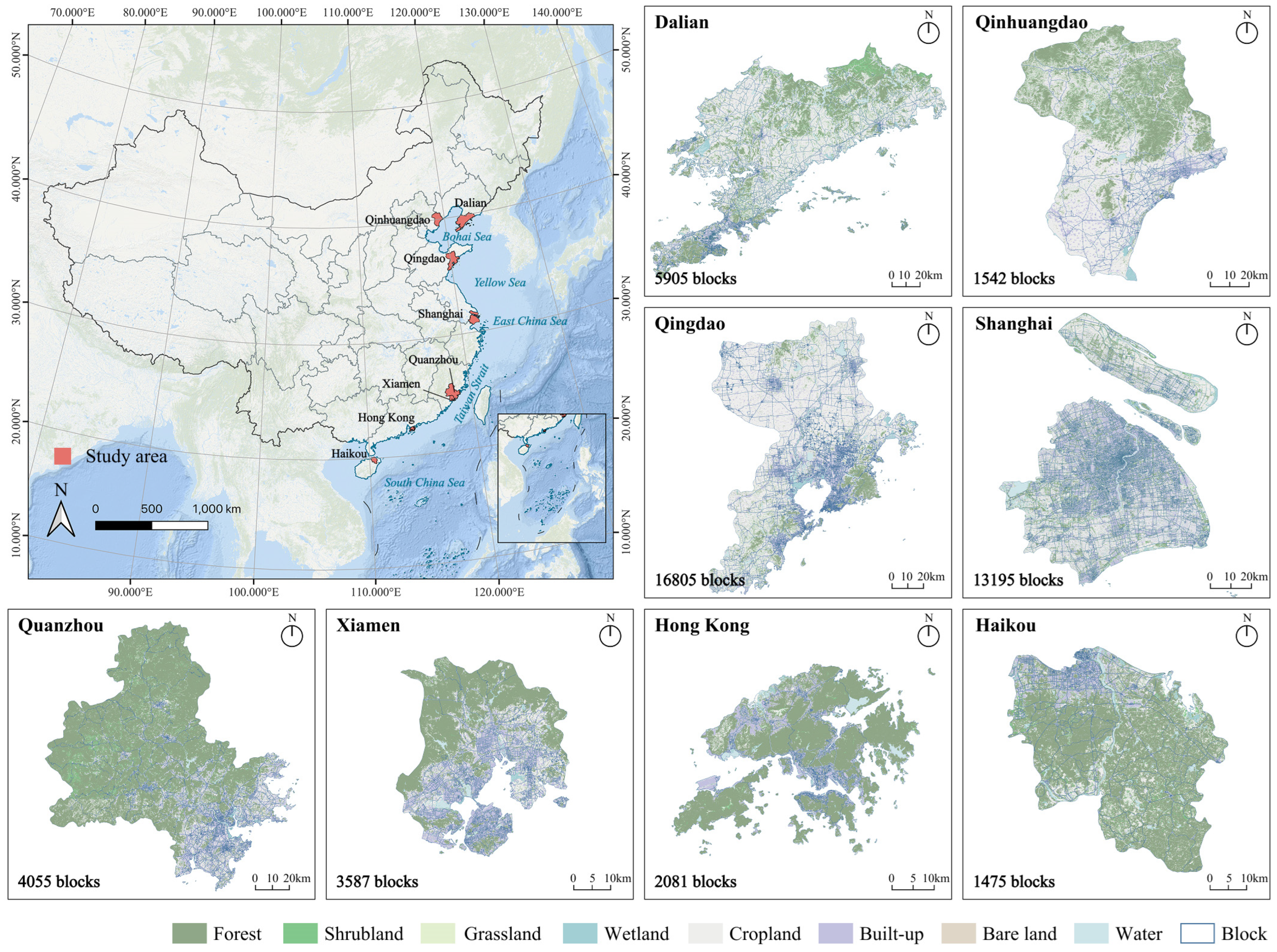
Figure 1. Study area.
Buildings 15 03544 g001
Figure 2. Methodological framework of this study.
Buildings 15 03544 g002
Figure 3. (a) Spatial distribution of various local climate zone types in 8 coastal cities; (b) Percentage of various local climate zone types in 8 coastal cities.
Buildings 15 03544 g003
Figure 4. Spatial distribution of Urban Heat Island Intensity (UHII) and descriptive statistical characteristics of UHII across various local climate zone types: (a) Dalian, (b) Qinhuangdao, (c) Qingdao, (d) Shanghai, (e) Quanzhou, (f) Xiamen, (g) Hong Kong, (h) Haikou.
Buildings 15 03544 g004
Figure 5. Pearson correlation matrix of influencing factors: (a) Dalian, (b) Qinhuangdao, (c) Qingdao, (d) Shanghai, (e) Quanzhou, (f) Xiamen, (g) Hong Kong, (h) Haikou.
Buildings 15 03544 g005
Figure 6. Comparative performance of machine learning models for UHII prediction. Each panel shows predicted vs. true values with training (blue) and test (red) data. Black dashed lines indicate perfect prediction; red lines show model fits.
Buildings 15 03544 g006
Figure 7. SHAP values of UHII impact factors: (a) Dalian, (b) Qinhuangdao, (c) Qingdao, (d) Shanghai, (e) Quanzhou, (f) Xiamen, (g) Hong Kong, (h) Haikou.
Buildings 15 03544 g007
Figure 8. The marginal effects of key factors on UHII: (a) Dalian, (b) Qinhuangdao, (c) Qingdao, (d) Shanghai, (e) Quanzhou, (f) Xiamen, (g) Hong Kong, (h) Haikou.
Buildings 15 03544 g008
Figure 9. Causal model structure and inference results: (a) Dalian, (b) Qinhuangdao, (c) Qingdao, (d) Shanghai, (e) Quanzhou, (f) Xiamen, (g) Hong Kong, (h) Haikou.
Buildings 15 03544 g009
Table 1. Study data details.
TypeSpatial ResolutionDataSources
Landsat 8 collection 2 product30 m1 June 2023 to
15 August 2023
USGS (https://earthexplorer.usgs.gov/)
Block division data-2022MSDCW Dataset
Building data-20203D-GloBFP: the first global three-dimensional building footprint dataset
Land use/cover data10 m2023GLC_FCS10: global 10 m landcover dataset
Population density data100 m2020A 100 m gridded population dataset of China’s seventh census using ensemble learning and geospatial big data
Tree height data10 m2023Sub-meter resolution canopy height maps
Nighttime light data100 m2023Global NPP-VIIRS-like nighttime light (2000–2023)
China coastline data-2023Openstreet map
Table 2. UHII influencing factors.
CategoryFactorsUnitAbbreviation
Biophysical parametersAlbedo-ALB
Normalized difference vegetation index-NDVI
Building morphologyBuilding density-BD
Building heightmBH
Sky view factor-SVF
Landscape IndicatorsAggregation index%AI
Patch cohesion index%COH
Landscape shape index-LSI
Shannon’s diversity index-SHDI
Split index-SPL
Tree heightmTH
GeographyDistance from seamDS
Social IndicatorsNighttime light-NTL
Population densitypeople/haPD
Table 3. LCZ classification accuracy in different cities.
DalianQinhuangdaoQingdaoShanghaiQuanzhouXiamenHong KongHaikou
Overall accuracy0.875440.869400.936050.803590.847580.853700.874590.85073
Kappa coefficient0.841690.846080.902530.753010.823080.831840.849290.82169
Table 4. XGBoost model performance metrics for 8 cities.
CityR2RMSE
Dalian0.7575727051.827308654
Qinhuangdao0.5871089752.270995959
Qingdao0.7976213281.95885009
Shanghai0.7589930972.36471014
Quanzhou0.4352343334.094986159
Xiamen0.4824267613.244835661
Hong Kong0.4539108162.926233686
Haikou0.4330732753.060312293
Disclaimer/Publisher’s Note: The statements, opinions and data contained in all publications are solely those of the individual author(s) and contributor(s) and not of MDPI and/or the editor(s). MDPI and/or the editor(s) disclaim responsibility for any injury to people or property resulting from any ideas, methods, instructions or products referred to in the content.