Article

Analysis and Prediction of Building Deformation Characteristics Induced by Geological Hazards

1
MOE Key Laboratory of Coast Civil Structure Safety, Tianjin University, Tianjin 300072, China
2
Department of Civil Engineering, Tianjin University, Tianjin 300072, China
3
College of Intelligence and Computing, Tianjin University, Tianjin 300072, China
*
Author to whom correspondence should be addressed.
Buildings 2025, 15(19), 3472; https://doi.org/10.3390/buildings15193472
Submission received: 19 August 2025 / Revised: 14 September 2025 / Accepted: 16 September 2025 / Published: 25 September 2025
(This article belongs to the Section Building Structures)

Abstract

To address the building settlement issues induced by an urban geological hazard in a northern city, this study utilizes settlement monitoring data from 16 high-rise buildings. The non-uniform temporal data were processed using the Akima interpolation method to construct a settlement prediction model based on a backpropagation (BP) neural network. The model’s predictive performance was validated against traditional approaches, including the hyperbolic and exponential curve methods, and was further employed to estimate the stabilization time of building settlements. Additionally, spatiotemporal characteristics of settlement behavior under the influence of geological hazards were investigated through a comparative analysis of deformation data across the building group. The results demonstrate that the BP neural network model achieves a 58.3% improvement in predictive accuracy compared to traditional empirical methods, effectively capturing the settlement evolution of buildings. The model also provides reliable predictions for the time required for buildings to reach a stable state. The temporal evolution of building settlement exhibits a distinct three-stage pattern: (1) an initial abrupt phase dominated by rapid water and soil loss; (2) a rapid settlement phase primarily driven by the consolidation of sandy and clayey soils; and (3) a slow consolidation phase governed by the prolonged consolidation of cohesive soils. Spatially, building deformations show significant regional heterogeneity, and the existence of potential finger-like preferential pathways for water and soil loss appears to exert a substantial influence on differential settlements.

1. Introduction

Urban geological hazards refer to hazardous events occurring within urban areas and their surroundings, triggered by natural geological processes or anthropogenic activities, which pose significant threats to buildings, infrastructure, public safety, and the ecological environment [1,2,3,4,5]. Due to the high population density and intensive economic activities in cities, such hazards are often characterized by their severity, wide impact, and substantial economic loss. Among these, land subsidence is a relatively overlooked type of urban geological hazard compared to active faults or landslides [6,7,8]. However, subsidence often exhibits irreversibility and cascading effects, leading to structural damage such as cracks, tilting, and differential settlement in buildings [9,10]. These impacts pose serious risks to urban safety and public property. Therefore, accurately predicting settlement trends and precisely analyzing deformation characteristics are not only essential for assessing structural risks but also form a critical basis for devising appropriate remediation strategies, playing a key role in ensuring engineering safety.
In 2023, a geological hazard occurred during deep well drilling in a northern city in China, causing localized land subsidence within a short time frame, which resulted in the tilting and settlement of several surrounding buildings. Following the event, particular engineering attention was directed to the stabilization time and the spatiotemporal distribution of building settlements. As a form of time-series data, building settlement records can be used to evaluate structural stability through various predictive approaches.
Empirical-formula-based methods are widely applied due to their simplicity and cost effectiveness [11]. For instance, Yang Tao et al. [12] proposed an improved settlement prediction model for embankments under staged construction on soft soil foundations based on the traditional hyperbolic method. Zhou Xin et al. [13] employed both exponential and hyperbolic methods to forecast embankment settlements and compared their predictive accuracies. Chen Shanxiong et al. [14] introduced the concept of the three-point method into the exponential model, proposing a modified exponential model for more accurate settlement prediction.
With the rapid advancement of machine learning, neural networks have gained widespread application in settlement prediction. Zhang Wenbo et al. [15] constructed a BP neural network-based model for building settlement forecasting, demonstrating high accuracy and stability, thereby providing guidance for settlement early warning. Peng Tao et al. [16] developed a hybrid BP neural network–grey system model for predicting soft foundation settlements. Case studies indicated the model’s effectiveness in short-term prediction and its practical value for estimating final settlements. Deng Chuanjun et al. [17] further enhanced BP neural network performance by integrating Particle Swarm Optimization (PSO) to optimize initial weights and thresholds, improving global convergence and resulting in a PSO-BP model with superior predictive capability. Comparative results showed that the PSO-BP model outperformed the traditional BP model in accuracy, offering an effective solution for precise settlement prediction. In addition, settlement data can also serve as a basis for analyzing spatiotemporal characteristics. Xu Qiang et al. [18] analyzed settlement monitoring data to identify the spatiotemporal evolution of land subsidence in the Yan’an New Area, providing valuable insights for future monitoring, urban planning, and hazard prevention. Similarly, Liu Zhenlin et al. [19] investigated settlement distribution characteristics in the Nansha District based on monitoring data, contributing scientific evidence for subsidence mitigation strategies.
To accurately evaluate building settlement under geological hazards and its implications for structural safety, this study introduces two major innovations. Innovation 1 is to address the challenges of non-uniform time intervals and missing values in monitoring data, and the Akima interpolation method was employed to complete the monitoring sequences. This approach preserves curve smoothness while effectively suppressing non-physical oscillations, thereby enhancing the quality and reliability of subsequent analyses and modeling. On this basis, a BP neural network was developed to establish a high-precision prediction model, enabling the accurate estimation of the time required for settlement stabilization. Regarding innovation 2, under the unique settlement conditions induced by urban geological hazards, the spatiotemporal distribution of settlement within building groups was systematically investigated based on both the temporal distribution of settlement data and the spatial arrangement of the structures. This analysis revealed the spatiotemporal evolution patterns of building deformation under specific hazard scenarios and provides a valuable reference for further exploration of disaster mechanisms.

2. Hazard Overview

2.1. Project Overview

The geological hazard occurred during deep drilling operations in China. The site is underlain by Ordovician carbonate rocks of the Paleozoic sequence, which have undergone long-term sedimentary interruptions, periods of exposure, leaching, and surface weathering. These processes have led to intense karstification in the upper part of the Ordovician limestone, making the formation highly susceptible to the development of cavities and fractures.
During drilling, a large karst cavity was encountered at a depth of approximately 1300 m within the Ordovician limestone. Significant drilling fluid loss occurred, allowing confined groundwater to carry Quaternary soil deposits into the cavity. This process triggered large-scale land subsidence at the ground surface.

2.2. Geological Conditions

The Quaternary strata in the study area are primarily composed of silty clay, clayey silt, silt, fine silty sand, and fine sand, with the Quaternary basement buried at approximately 300 m. Beneath the Quaternary lies the Neogene system, which can be subdivided into two main formations. From 300 to 1150 m, the strata belong to the Minghuazhen Formation, characterized by alternating layers of fine sand, silty sand, and clay. From 1150 to 1300 m, the Guantao Formation comprises gray-green to gray-white sandstones and conglomeratic sandstones interbedded with brownish-red mudstones of variable thickness; the lower portion transitions into light gray, medium-to-coarse-grained gravelly sandstone. Underlying these Neogene deposits is the Ordovician limestone of the Paleozoic era. Due to long-term sedimentary discontinuities, exposure, leaching, and surface weathering, the upper Ordovician carbonate rocks have undergone intense karstification, making them highly prone to the development of cavities and fractures.
The Quaternary strata in the study area are mainly composed of an irregular interbedded sequence of sandy soils and cohesive soils, deposited under fluvial–proluvial, alluvial, alluvial–marine, and marine environments. Vertically, the deposits display distinct variations in color, the sand–clay ratio, and concretion distribution and can be divided into four stratigraphic units corresponding to the Early Pleistocene, Middle Pleistocene, Late Pleistocene, and Holocene. The Holocene deposits are dominated by grayish-yellow, grayish-brown, and yellowish-brown silty clay with minor occurrences of blackish-gray clay and sandy clay, interbedded with thin silt layers. The Late Pleistocene sequence consists of irregular interbeds of yellow-gray, dark-gray, and blackish-gray silty clay, silty sand, fine sand, and silt, within which two marine transgressive layers are widely developed. The Middle Pleistocene deposits comprise gray to light-gray fine sand and silt interbedded with yellow, gray, brown, and grayish-green silty clay and sandy clay, locally containing lenses of dark-gray to blackish-gray clay. Irregular alternations of brown, yellowish-brown, and grayish-green clay with sand and silt are also present, characterized by clay dominance with only minor silty clay and sandy clay, while localized reddish-brown clay layers can be observed.
Hydrogeologically, the Quaternary system contains five major aquifer groups. The shallowest is an unconfined aquifer within the top 40 m, mainly composed of fine to silty sand, with a typical groundwater table at depths of 0–2 m. Below this, the first confined aquifer, between 40 and 102 m, is a semi-confined system dominated by clayey silt, silty sand, and fine sand, with a groundwater level generally around 8 m deep. The second to fourth confined aquifers, located between 102 and 300 m, consist primarily of silty and fine sand layers. Some sections contain laterally continuous, thick sand beds, and groundwater levels in these confined units range between 17 and 65 m below the surface.

2.3. Monitoring Plan

Following the occurrence of the geological hazard, settlement monitoring was promptly initiated to obtain a comprehensive understanding of the structural response of buildings within the affected area. Monitoring points were installed on 16 high-rise buildings located in the core zone. During the emergency response phase, settlement measurements were conducted daily to capture rapid deformation changes. As the situation stabilized, the monitoring frequency was reduced to once every 7 days. Once no significant additional settlement was observed, the frequency was further reduced to a 30-day interval. The spatial distribution of the monitored buildings is shown in Figure 1.

3. Prediction of Settlement Stabilization

3.1. Prediction Method

(1)
Hyperbolic method
The hyperbolic method [11] relies on measured data of foundation settlement for settlement prediction, mainly fitting settlement amount–time–load. In practical engineering, the calculation of the final settlement amount of soft soil foundations is mainly carried out according to the following Formula (1):
s t = s 0 + t t 0 α + β ( t t 0 )
The following formula is derived from Formula (1):
t t 0 s t s 0 = α + β ( t t 0 )
In the formula, S t represents the settlement value at time t ; t 0 is the selected initial time point; S 0 is the foundation settlement amount corresponding to the time point t 0 ; and α   and   β are settlement prediction coefficients related to the foundation and load, which can be obtained through fitting.
(2)
Exponential curve method
The exponential curve prediction method [11], also known as the three-point method, is derived from the theoretical equation of the degree of consolidation, which states that the average degree of consolidation and consolidation time of ideally saturated soil under constant load follow an exponential function relationship:
S t = S 1 A e B t
In the formula, the theoretical value of A is 8 / π 2 ; B is the drainage distance; and S is the final settlement amount of the foundation when t . B and S can be obtained from three points, t 1 , S 1 , t 2 , S 2 , and t 3 , S 3 , with equal time intervals and long intervals using Formulas (4) and (5).
S = S 3 S 2 S 1 S 2 S 3 S 2 S 2 S 1 S 3 S 2
B = 1 t 1 t 2 × ln S 2 S 1 S 3 S 2
(3)
BP Neural Network
The backpropagation (BP) neural network [20] is a type of multilayer feedforward neural network that utilizes the error backpropagation algorithm for training. To date, the BP algorithm has become the most widely used neural network approach in the field of settlement prediction [21]. A typical BP neural network consists of three or more layers, each composed of multiple neurons. Every neuron receives input from the previous layer and transmits its output to the next layer. The nodes within the network are classified into two types: input nodes and computational nodes. Each computational node can receive multiple signals from the preceding layer but produces only a single output.
The BP neural network operates under a supervised learning paradigm. During training, input samples are fed into the network, and signals are propagated forward through the layers to produce an output. The difference between the predicted output and the expected (target) output is calculated as an error, which is then propagated backward through the network to adjust the weights and biases of the neurons. This process is repeated iteratively, and with each iteration, the network minimizes the error, gradually aligning the predicted outputs with the expected values.
(4)
LSTM Neural Network
LSTM networks are a specialized type of RNN designed to address the long-term dependency problem commonly encountered by standard RNNs when modeling long-sequence data. Although RNNs excel at handling sequential data, such as time series and natural language, they have the vanishing or exploding gradient problem during backpropagation through time, which hampers their ability to learn dependencies between distant time steps.
The core innovation of the LSTM lies in its memory cells (cell states) and gating mechanisms. The memory cell functions as a “conveyor belt” that can transmit relevant information over extended time intervals. The gating mechanisms precisely regulate the information flow and comprise three primary gates: the forget gate, which determines which historical information in the memory cell should be discarded, the input gate, which controls the updating of new information into the memory cell, and the output gate, which determines the output at the current time step based on the updated cell state. This sophisticated gating architecture enables the LSTM to selectively retain long-term information, update new inputs, and generate corresponding outputs. Consequently, LSTM significantly enhances the capacity of the model to capture long-range dependencies in sequences. LSTM has been successfully used in machine translation, speech recognition, and time-series forecasting.

3.2. Data Selection and Processing

Building F, which experienced the most significant impact from the hazard within the study area, was selected for detailed analysis. According to relevant engineering standards [22], a building is considered to have reached a stable settlement state when the maximum daily settlement rate over the last 100 days falls below 0.01–0.04 mm/day. Based on this criterion, both the total settlement and the time to stabilization of Building F were predicted.
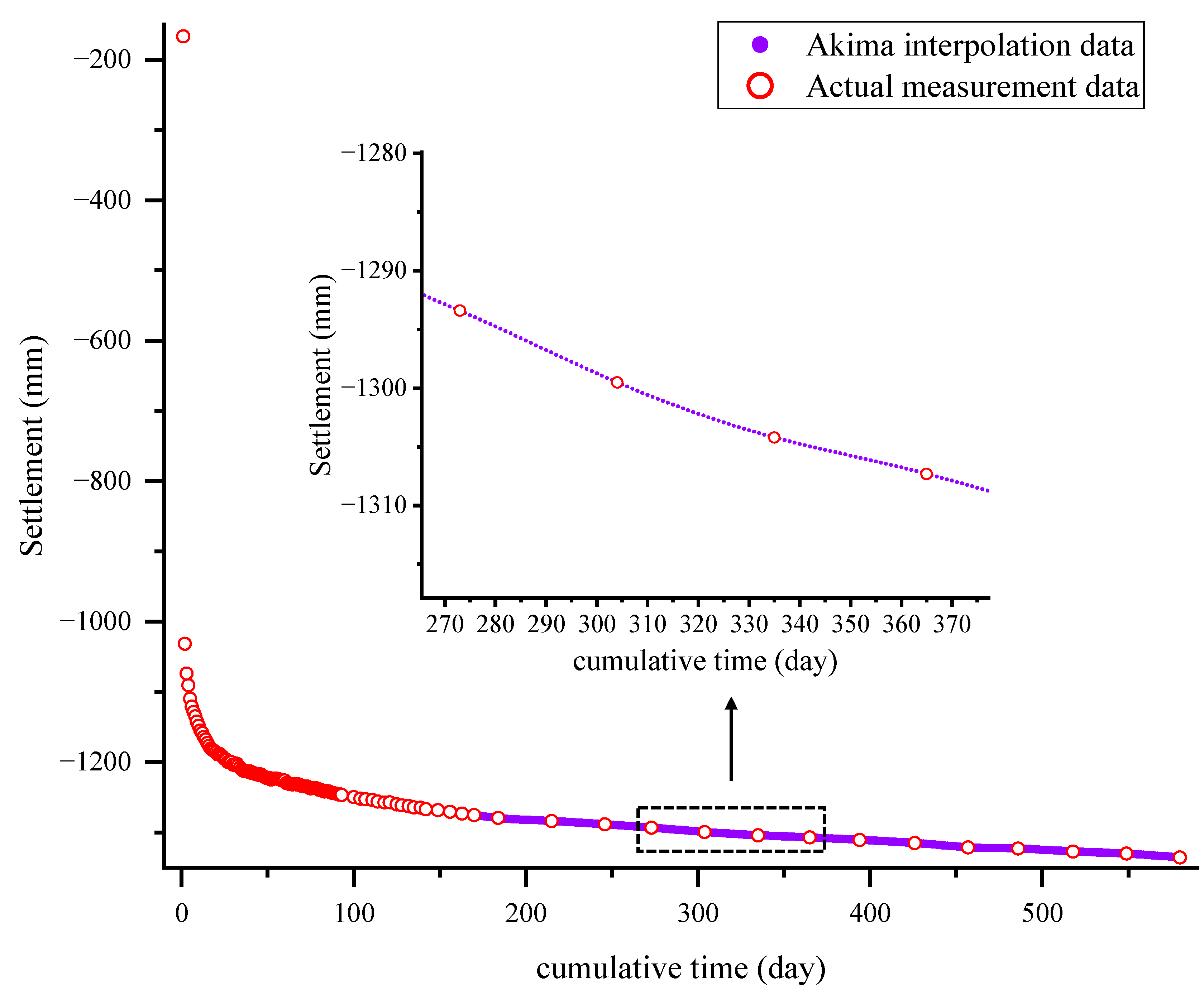
Due to variations in monitoring frequency during different stages of the hazard response, the raw settlement data exhibited pronounced non-uniform temporal intervals. The Akima interpolation method [23] was adopted to preprocess the settlement monitoring data with non-uniform time intervals and missing records. Compared with conventional interpolation techniques such as linear interpolation, cubic spline interpolation, or polynomial fitting, Akima interpolation offers several advantages that are particularly suitable for building settlement data. Specifically, it (i) suppresses non-physical oscillations that frequently occur in cubic spline interpolation, (ii) provides smooth curves without overshooting, which preserves the physical rationality of settlement processes, (iii) exhibits robustness to local anomalies, ensuring that individual outliers do not excessively influence the overall curve, and (iv) performs well with irregularly spaced data, which is common in field monitoring. The Akima interpolation method was employed to transform the non-uniform time series into an evenly spaced dataset with a fixed interval of one day, as shown in Figure 2. As a result, a total of 580 interpolated data points were obtained for subsequent modeling and analysis.
A total of 580 datasets were divided into a training group (1–550) and a prediction group (551–580). The training set was used to establish three models: a hyperbolic model, an exponential model, and a BP neural network model. For the BP neural network, the training group was further split into a training set and a testing set to evaluate the generalization ability of the model and prevent overfitting.
The interpolated data were then imported into the BP neural network time-series prediction model for training. To determine the optimal hyperparameters of the BP neural network, a grid search approach was employed. Specifically, different combinations of prediction horizon, number of hidden neurons, learning rate, and maximum iterations were systematically tested within predefined ranges. Model performance under each parameter setting was evaluated using root mean square error (RMSE) and mean absolute error (MAE). The final configuration (prediction horizon = 10, hidden neurons = 8, maximum iterations = 2000, gradient threshold = 1 × 10⁻⁶, and initial learning rate = 0.005) was selected, as it achieved the lowest prediction error while maintaining computational efficiency.
Subsequently, the remaining 30 samples (prediction set) were used as unseen data to evaluate the predictive performance of the three models. The outputs of the hyperbolic, exponential, and BP neural network models were compared against the actual measured values to assess and validate their prediction accuracy.

3.3. Model Evaluation Indicators

The mean absolute error (MAE), root mean square error (RMSE), and coefficient of determination (R2) are used as evaluation indicators for model performance. The calculation formulas for MAE, RMSE, and R2 are as follows:
M A E = 1 N i = 1 N Y i Y i
R M S E = 1 N i = 1 N ( Y i Y i ) 2
R 2 = 1 i = 1 N ( Y i Y i ) 2 i = 1 N ( Y i Y ¯ ) 2
where N is the number of data samples; Yi denotes the predicted settlement value of the existing building; Yi represents the measured settlement value; and Y is the mean of the measured settlement values.

3.4. Model Results and Analysis

To evaluate the accuracy of the developed hyperbolic curve model, exponential curve model, and BP neural network model, the predicted settlement values from each model were compared against the measured data. Model performance was assessed using mean absolute error (MAE) and root mean square error (RMSE) to quantify prediction accuracy, while the coefficient of determination (R2) was calculated to evaluate model stability. The evaluation metrics for all models are summarized in Table 1.
According to the results presented in Table 1, the BP neural network model outperforms the hyperbolic model, the exponential curve model, and the LSTM neural network model in terms of MAE, RMSE, and R2. This indicates that the BP neural network achieves higher accuracy and greater stability in predicting building settlement. These findings further demonstrate that the BP neural network provides a distinct advantage in forecasting settlement induced by urban geological disasters.
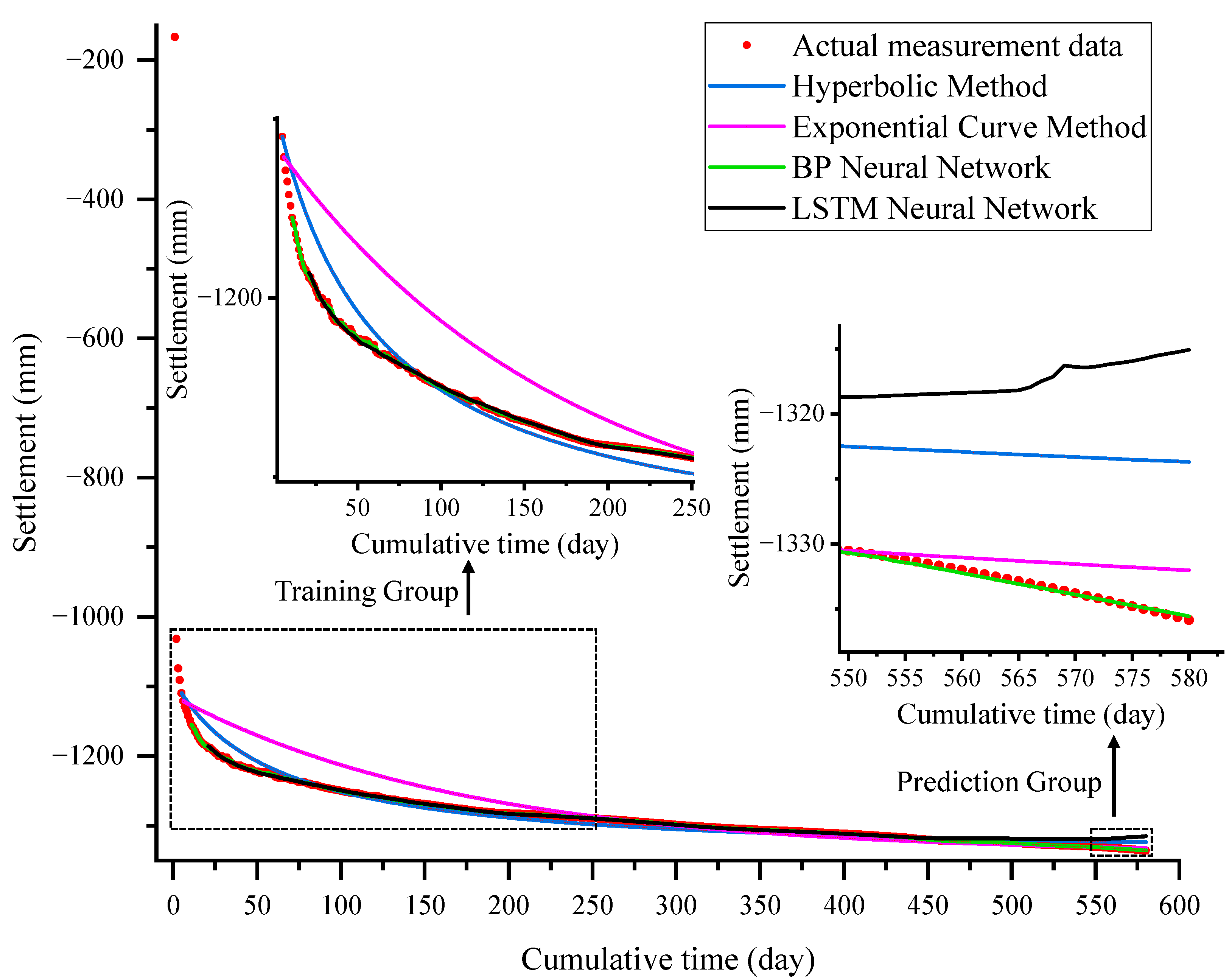
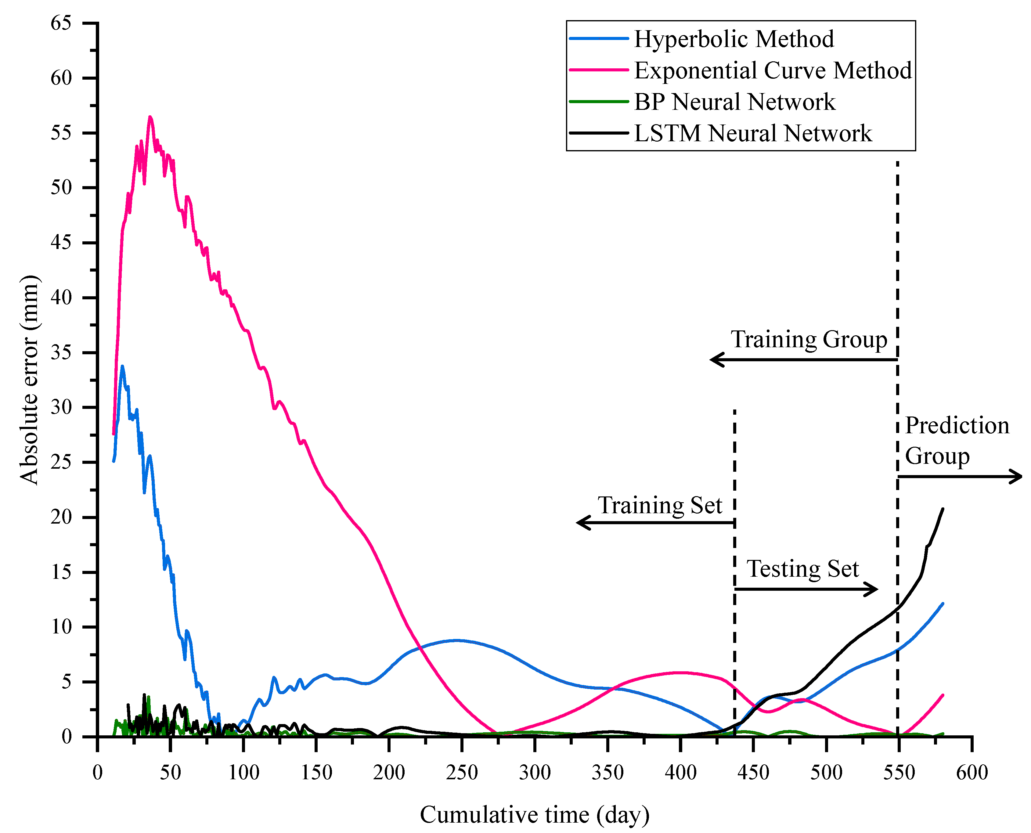
To provide a more intuitive comparison of the predictive performance of the different models, the predicted and observed values are plotted in Figure 3, while the absolute error curves are shown in Figure 4.
As illustrated in Figure 3, the overall trends of the predicted values and the measured values are consistent across all four models. However, significant differences can be observed in the training group. The exponential curve model exhibits poor performance in the early stage (0–250 days), with large deviations from the measured values; the hyperbolic model also shows a noticeable bias within the first 50 days. The LSTM neural network demonstrates excellent fitting performance on the training set, but its accuracy decreases sharply on the testing set, suggesting severe overfitting. In contrast, the BP neural network achieves good fitting performance on both the training and testing sets. As further supported by the statistical results in Table 2, the LSTM model achieves an R2 of 0.999 on the training set but only 0.342 on the testing set, whereas the BP neural network maintains R2 values of 0.982 and 0.968 on the training and testing sets, respectively. This highlights the overfitting problem of the LSTM model and the stronger generalization ability of the BP model. From the prediction group, it can also be observed that the exponential curve model and the BP neural network produce results that are more consistent with the measured values, reliably reflecting the future stabilization trend of settlement, while the LSTM and hyperbolic models deviate significantly, showing insufficient predictive capability.
Figure 4 further compares the absolute errors of the four models. The results reveal that both the hyperbolic and exponential curve models exhibit substantial errors during the training group, with fluctuations showing a repeated pattern of increase and decrease. The maximum error of the hyperbolic model reaches 33.3 mm, while that of the exponential model reaches 40.17 mm. During the prediction phase, the errors of both models gradually increase, eventually exceeding 4.7 mm, with maximum values of up to 12.1 mm. Although the LSTM model maintains relatively small errors in the training group, its errors accumulate considerably in the testing and prediction phases, again confirming its overfitting problem. By contrast, the BP neural network shows only slight fluctuations in error during training, with consistently high predictive accuracy. Although the errors in the prediction phase also show a gradual increasing trend, the magnitudes remain very small, making the BP model markedly superior to the other approaches.
In summary, the BP neural network model not only demonstrates higher accuracy and stability in building settlement prediction but also exhibits stronger generalization capability. Therefore, it offers significant advantages in addressing settlement prediction problems associated with urban geological disasters.
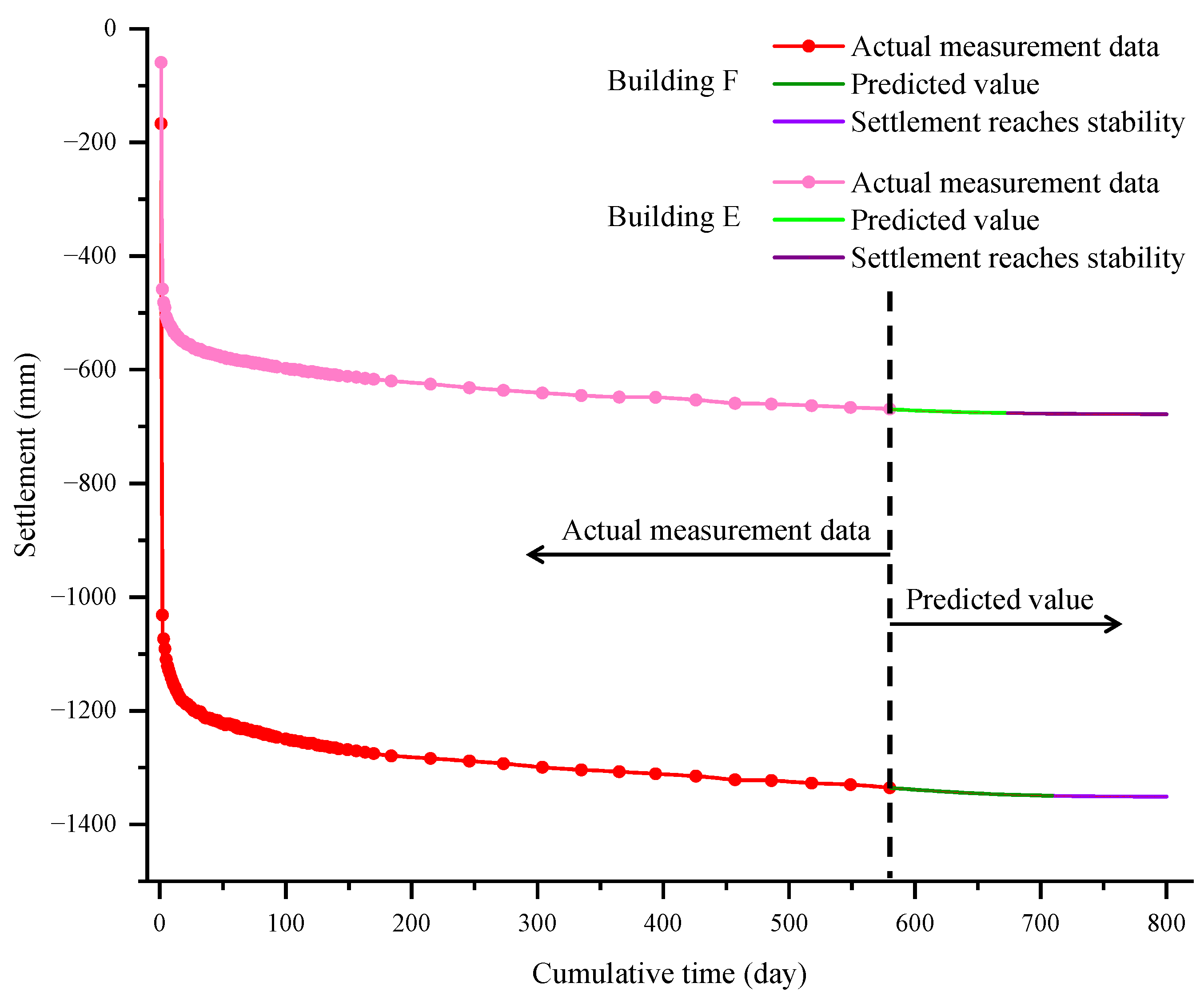
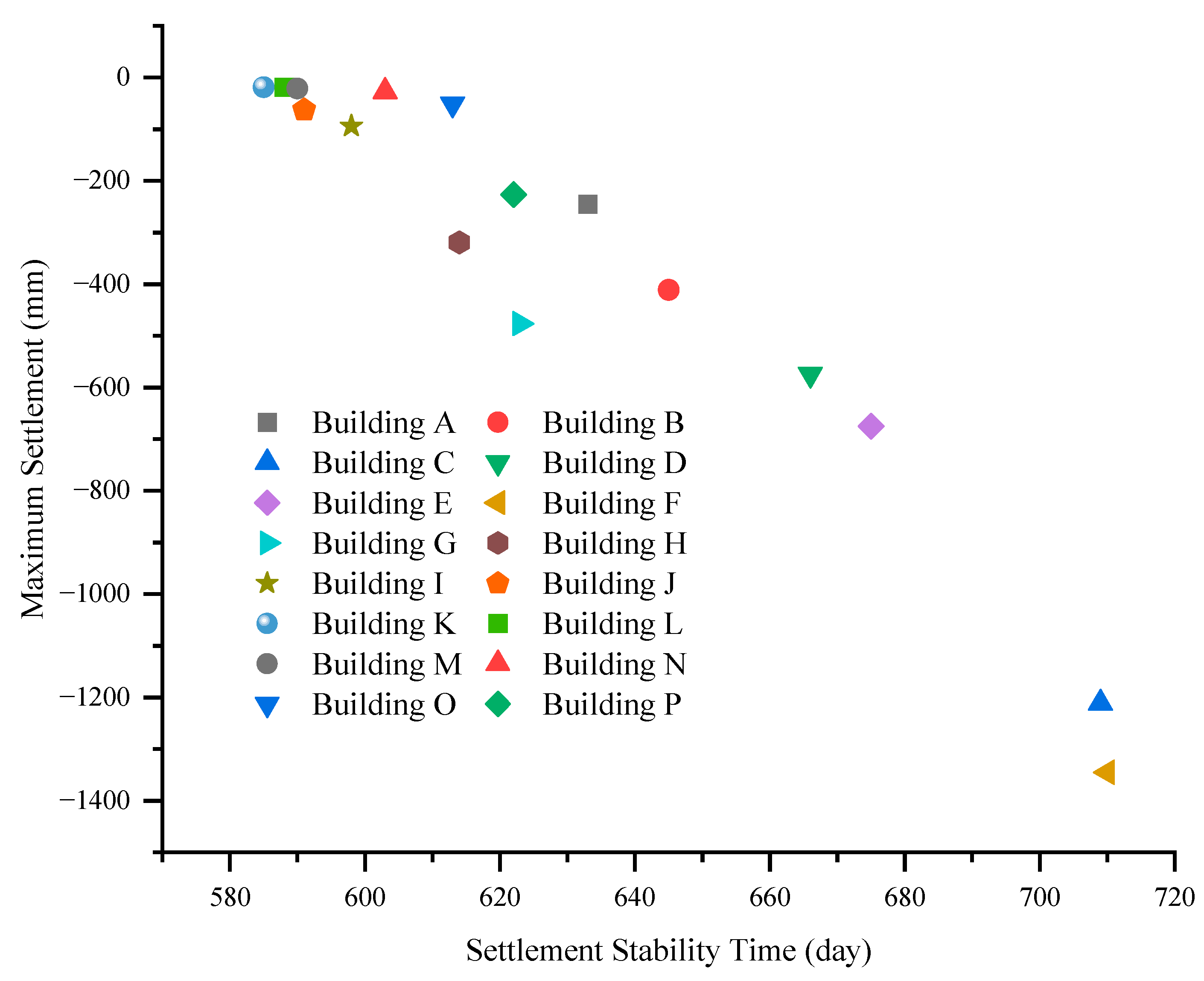
The trained BP neural network model was applied to predict the settlement of Buildings E and F to determine their stabilization times. The predicted settlement curves are presented in Figure 5. As shown, both buildings exhibit a trend of increasing settlement with a gradually decreasing rate. Specifically, the daily settlement rate of Building E falls below 0.04 mm/day at approximately 675 days, while Building F reaches this threshold around 710 days. Following these points, the settlement rates continue to decline, indicating that both buildings meet the defined stabilization criteria. Subsequently, stability predictions were conducted for all other buildings, and the stability time and maximum settlement are shown in Figure 6.

4. Deformation Characteristics of Buildings

4.1. Temporal Characteristics of Deformation

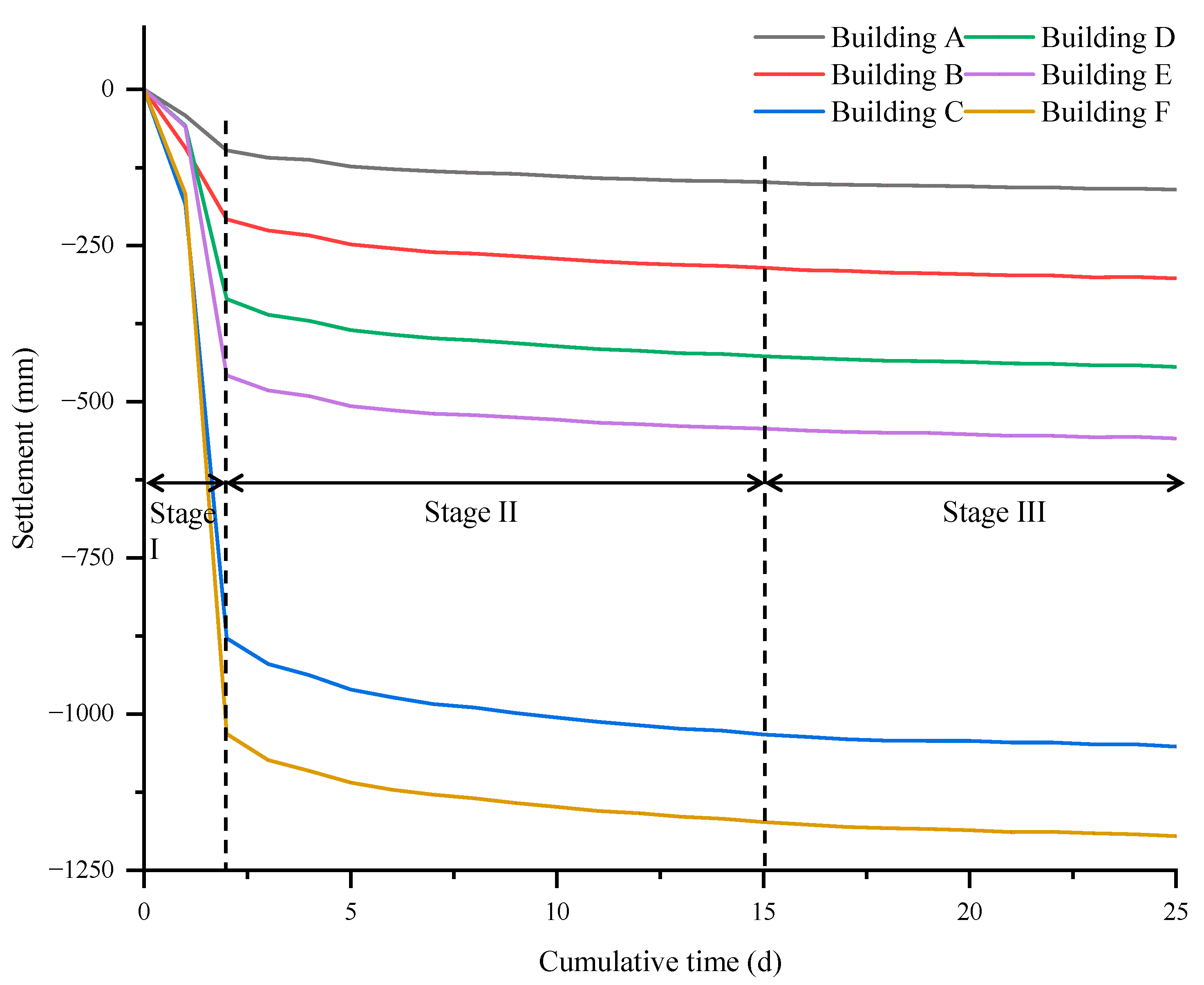
To investigate the temporal evolution of building settlement, six representative buildings (A–F) that exhibited significant deformation were selected. While other structures in the area also display similar settlement characteristics, these six buildings present the patterns more distinctly in the monitoring data, as illustrated in Figure 7. The strata affected in this area are mainly composed of sand and clay, whose geotechnical characteristics differ substantially: sand is highly erodible and consolidates rapidly, whereas clay is more resistant yet consolidates extremely slowly. Based on monitoring data, together with the underlying causes of the disaster and the contrasting properties of sand and clay, the settlement process of the buildings can be divided into three stages:
(1) Stage I: During this stage, buildings experienced significant settlement within a short period, primarily due to extensive sand loss triggered by the disaster. This phase lasted for approximately two days.
(2) Stage II: In this stage, the settlement pattern of the buildings shifted compared with Stage I, transitioning from abrupt short-term settlement to rapid settlement with an average daily rate of several millimeters. This process was attributed to the combined consolidation and creep of sand and clay, induced by soil disturbance and changes in the groundwater level. The duration of this stage was approximately from Day 2 to Day 15.
(3) Stage III: The settlement rate gradually decreased, and the buildings entered a phase of slow but persistent settlement. This pattern reflects the rapid completion of consolidation in the sand layer, owing to its high permeability and low compressibility, contrasted with the prolonged consolidation of the clay layer due to its low permeability and high compressibility. This phase extended beyond Day 15.
Together, these three stages characterize the overall development of building settlement in the affected area.

4.2. Spatial Characteristics of Deformation

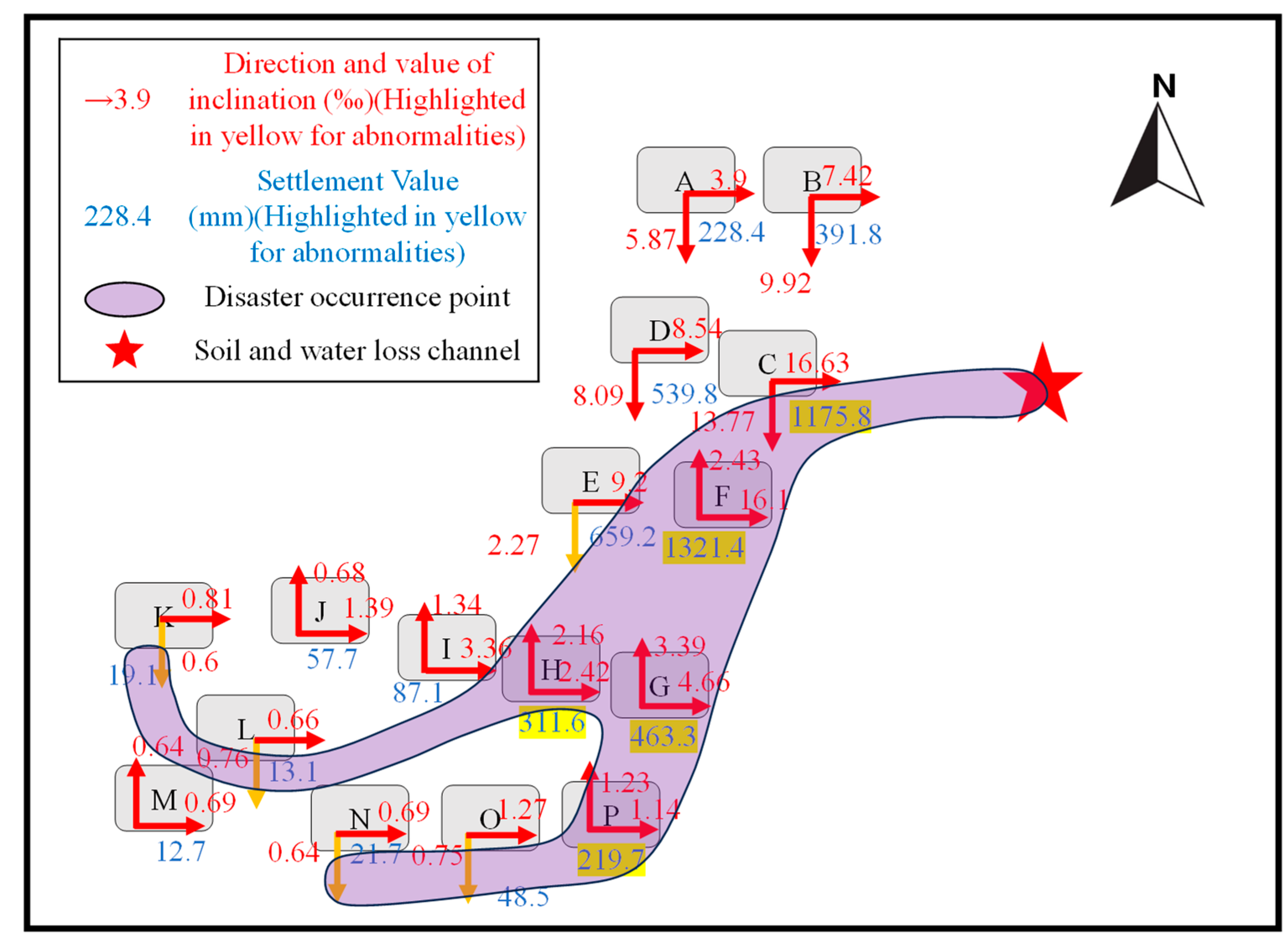
As illustrated in Figure 8, the settlement and tilt measurements of the 16 monitored buildings within the study area exhibit considerable variability.
Firstly, the deformation characteristics of six buildings (A through F) located within 300 m of the hazard epicenter were analyzed. Buildings B, C, and F, situated closer to the hazard site, experienced larger settlements compared to Buildings A, D, and E. Interestingly, although the distances from the hazard point to Buildings B, C, and F do not differ significantly, an anomalously large settlement exceeding 1 m was observed at Buildings C and F on the southeastern side of the area. This is notably higher than the 391.8 mm settlement recorded at Building B. Furthermore, comparison among Buildings A, B, D, and E revealed that the southern portion of the region experienced substantially greater settlement than the northern part. Regarding tilt directions, five out of the six buildings showed inclination toward the hazard point. The maximum tilt was recorded at Building C, with an eastward tilt of 16.63‰. In contrast, Building E exhibited a southward tilt of 2.27‰ away from the hazard site. Comparing the tilts of Buildings C and F, Building C displayed a southward tilt of 13.77‰, whereas Building F showed a much smaller northward tilt of only 2.43‰.
Secondly, the deformation of ten buildings (G through P) located beyond 300 m from the hazard site was analyzed. Buildings G to J are arranged at increasing distances from the hazard point, each approximately 30 m apart. Both Buildings G and F experienced settlements exceeding 300 mm, whereas Buildings I and J recorded settlements below 90 mm. A similar pattern was observed among Buildings N to P: Building P settled by 219.7 mm, while Buildings N and O settled by only 21.7 mm and 48.5 mm, respectively. Spatially, although Buildings H, G, and P on the eastern side are closer to the hazard site, the distance alone does not explain the observed settlement differences of up to hundreds of millimeters between buildings. The eastern corner of the monitored region exhibited significantly greater settlement than other areas. Tilt data for these ten buildings showed that six inclined toward the hazard site, with the maximum tilt of 4.66‰ recorded at Building G. The remaining four buildings exhibited southward tilts away from the hazard point.
In the study area, multiple buildings exhibited settlement and tilting, which contradicts the conventional understanding that deformation patterns typically follow a “well-centered” distribution, i.e., settlement decreases with increasing distance from the well, and tilting is oriented toward the well. The fundamental cause of these anomalies lies in severe water and soil loss, whose direction and magnitude directly control the spatial distribution and intensity of both settlement and tilting. The investigation revealed that, following the onset of the disaster, water and soil loss within the core zone did not diffuse radially and uniformly outward from the failure point. Instead, it developed into finger-like preferential pathways of erosional loss, which in turn produced the observed abnormal building settlements and tilts. Specifically, substantial soil depletion occurred along these preferential pathways, inducing pronounced localized surface subsidence, such that buildings situated directly above the pathways experienced markedly greater settlement. Meanwhile, adjacent structures, subjected to differential settlement across the pathway margins, exhibited anomalous tilting directions.
In summary, by integrating building deformation data associated with these finger-like preferential pathways of water and soil loss, the orientation and extent of the subsurface erosion channels can be reconstructed in reverse.

5. Conclusions

This study takes a representative urban geological disaster as a case and systematically analyzes the settlement evolution of buildings under disaster conditions. To address the issues of irregular monitoring intervals and missing data, the Akima interpolation method was employed to optimize and complete the monitoring series. This approach maintains curve smoothness while effectively suppressing non-physical oscillations. On this basis, a high-precision BP neural network prediction model was developed to quantitatively estimate the stabilization time of building settlement. Furthermore, by integrating the temporal distribution characteristics of settlement data with the spatial layout of the buildings, the spatiotemporal distribution patterns of building settlements induced by urban geological disasters were comprehensively investigated. The main findings are as follows:
  • For building settlements triggered by urban geological disasters, the integration of the Akima interpolation method with a BP neural network effectively overcomes the adverse effects of data discontinuity. Compared with traditional empirical-formula-based methods, this combined approach more accurately captures settlement trends and achieves significantly higher prediction accuracy. The prediction results derived from the model provide a scientific basis for the dynamic assessment of building stability, thereby supporting the timely optimization and adjustment of restoration and reinforcement schemes to ensure construction safety.
  • The building settlements induced by this geological disaster exhibit pronounced temporal staging and spatial heterogeneity. Substantial water–soil loss in the early stage, coupled with the different consolidation rates of sandy and clayey soils in the middle and late stages, jointly produced a three-phase settlement evolution process. In addition, water–soil loss was frequently accompanied by the development of finger-like preferential pathways, which aggravated localized settlement and caused significant spatially differentiated deformation within the building cluster.

Author Contributions

X.C.: Project Administration, Supervision, Conceptualization. Q.S.: Writing—Original Draft, Visualization, Methodology, Investigation, Conceptualization. J.L.: Conceptualization, Project Administration. J.S.: Writing—Review and Editing, Methodology, Conceptualization, Investigation. T.L.: Data Curation. G.Z.: Project Administration, Supervision. All authors have read and agreed to the published version of the manuscript.

Funding

This work was supported by the China Postdoctoral Science Fund (Pre-Station) (Grant No. 2023TQ0241), the National Natural Science Foundation of China (Grant No. 52178343), and the National Science Foundation for Distinguished Young Scholars of Tianjin (Grant No. 24JC1Q1C00170). Their support is gratefully acknowledged.

Data Availability Statement

The data presented in this study are available on request from the corresponding author due to that the datasets generated and/or analyzed during the current study are not publicly available owing to the confidentiality of the project.

Conflicts of Interest

The authors declare no conflict of interest.

References

  1. Yu, B.F.; Yan, J.X.; Li, Y.A.; Xing, H.X. Urban construction promotes geological disasters: Evidence from prediction of future urban road collapse scenario in Hangzhou, China. Georisk 2025, 19, 661–681. [Google Scholar] [CrossRef]
  2. Santi, P.; Manning, J.; Zhou, W.; Meza, P.; Colque, P. Geologic hazards of the Ocona river valley, Peru and the influence of small-scale mining. Nat. Hazards 2021, 108, 2679–2700. [Google Scholar] [CrossRef]
  3. Li, Z.; Zhang, Y.; Liang, S. Urban geological hazards and human engineering activities in Lanzhou City. J. Lanzhou Univ. Nat. Sci. 2014, 50, 588–593. [Google Scholar]
  4. Li, Y.; Zhuang, Y.; Cai, G.; Liu, S.; Zhang, Z. Urban geological work-A new area of national geological work. Geol. Bull. China 2003, 22, 589–596. [Google Scholar]
  5. Duan, X.; Zhu, J.; Dong, Q.; Chen, Z. Discussion of the Correlation between Human Engineering Activities and Geological Disasters in Yan'an Area. J. Catastrophology 2017, 32, 106–110. [Google Scholar]
  6. Yin, Y.; Zhang, Z.; Zhang, K. Land subsidence and countermeasures for its prevention in China. Chin. J. Geol. Hazard Control. 2005, 16, 1–8. [Google Scholar]
  7. Yi, L.; Wang, J.; Shao, C.; Guo, J.; Jiang, Y.; Bo, L. Land Subsidence Disaster Survey and Its Economic Loss Assessment in Tianjin, China. Nat. Hazards Rev. 2010, 11, 35–41. [Google Scholar] [CrossRef]
  8. Jin, J.; Pan, M. Status of Land Subsidence Damages and Strategy for Disaster Prevention and Mitigation in China. J. Catastrophology 2007, 22, 117–120. [Google Scholar]
  9. Chen, D.; Tang, L.; Guo, J. Analysis and treatment of an uneven settlement accident of a residential building. Ind. Constr. 2011, 41, 136–139. [Google Scholar]
  10. Chen, D.; Cao, R.; Shi, C.; Dong, S.; Hu, J. Reason and treatment of an uneven foundation settlement accident of a bottom frame structure house. Build. Struct. 2015, 45, 43. [Google Scholar]
  11. Pan, L.; Xie, X. Observational settlement prediction by curve fitting methods. Rock Soil Mech. 2004, 25, 1053–1058. [Google Scholar]
  12. Yang, T.; Li, G.; Yang, W. Settlement prediction of stage constructed embankment on soft groundbased on the hyperbolic method. Rock Soil Mech. 2004, 25, 1551–1554. [Google Scholar]
  13. Zhou, X.; Zhang, Q.; Zeng, Y.; Sun, G. Contrastive Analysis on Exponential Fitting and Hyperbolic Fitting in Settlement Prediction of Soft Foundation. Explor. Eng. 2011, 38, 51–53+58. [Google Scholar]
  14. Chen, S.; Wang, X.; Xu, X.; Yu, F.; Qin, S. Three-point modified exponential curve method for predicting subgrade settlements. Rock Soil Mech. 2011, 32, 3355–3360. [Google Scholar]
  15. Zhang, W.; Guo, Y. Prediction model of building settlement based on BP neural network. Eng. Surv. Mapp. 2013, 22, 52–56. [Google Scholar]
  16. Tao, P.; Anying, Y.; Xing, L.; Qin, Y. Prediction of soft ground settlement based on BP neural network-grey system united model. Rock Soil Mech. 2005, 26, 1810–1814. [Google Scholar]
  17. Deng, C.; Ouyang, B.; Chen, Y. A buliding settlement prediction model based on PSO-BP neural network. Sci. Surv. Mapp. 2018, 43, 27. [Google Scholar]
  18. Xu, Q.; Pu, C.; Zhao, K.; He, P.; Zhang, H.; Liu, J. Time Series InSAR Monitoring and Analysis of Spatiotemporal Evolution Characteristics of Land Subsidence in Yanan New District. Geomat. Inf. Sci. Wuhan Univ. 2021, 46, 957–969. [Google Scholar]
  19. Liu, Z.; Wang, Y.; Ke, X.; Luo, X. Distribution characteristics and causes of land subsidence in Nansha District, Guangzhou. Chin. J. Geol. Hazard Control. 2023, 34, 49–57. [Google Scholar]
  20. Basheer, I.A.; Hajmeer, M. Artificial neural networks: Fundamentals, computing, design, and application. J. Microbiol. Methods 2000, 43, 3–31. [Google Scholar] [CrossRef]
  21. Wang, Z.-L.; Li, Y.-C.; Shen, R.F. Correction of soil parameters in calculation of embankment settlement using a BP network back-analysis model. Eng. Geol. 2007, 91, 168–177. [Google Scholar] [CrossRef]
  22. JGJ8-2016; Code for Deformation Measurement of Building and Structure. Ministry of Housing and Urban-Rural Development of the People’s Republic of China: Beijing, China, 2007.
  23. Akima, H. A new method of interpolation and smooth curve fitting based on local procedures. JACM 1970, 17, 589–602. [Google Scholar] [CrossRef]
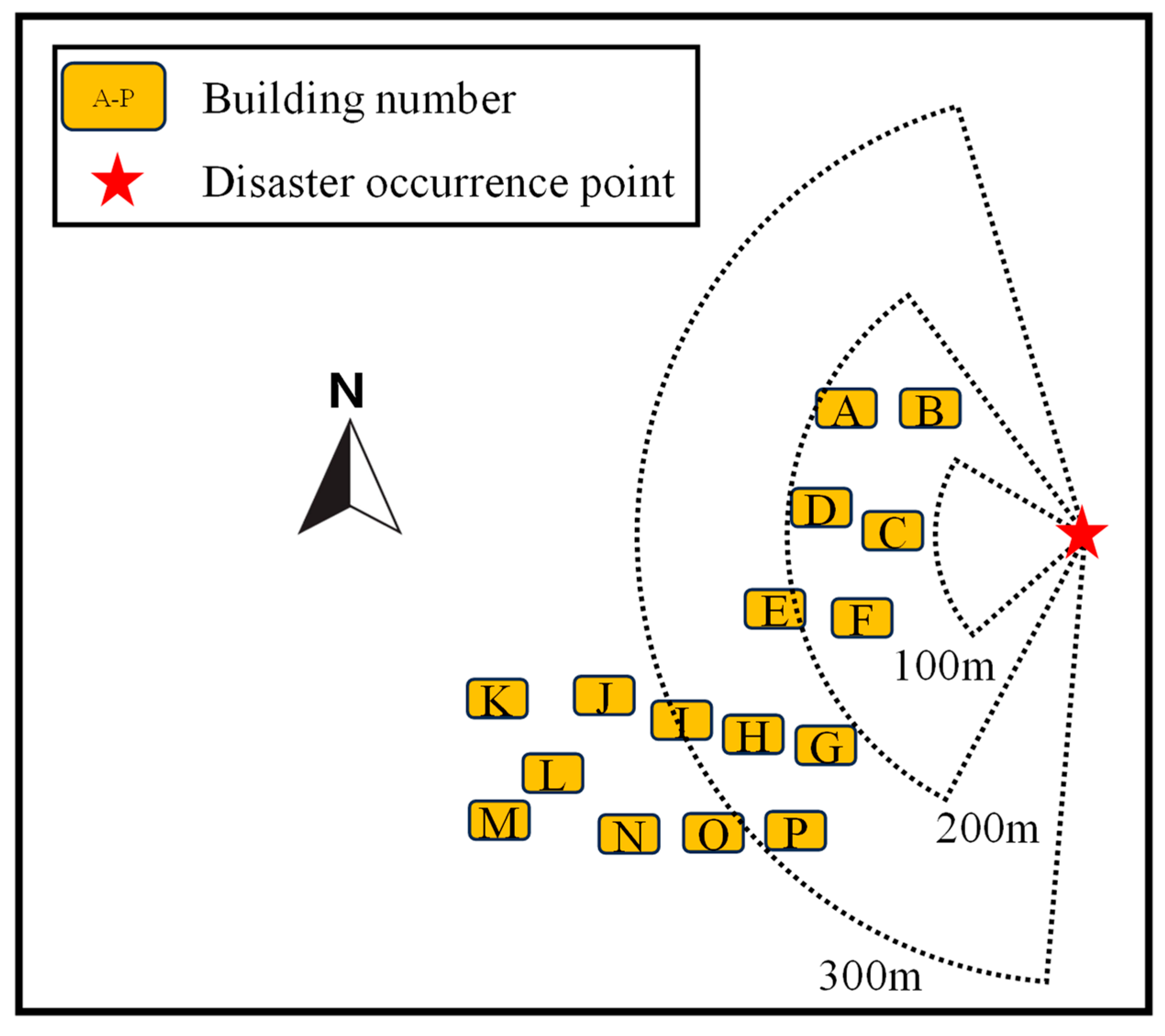
Figure 1. Distribution of high-rise buildings.
Buildings 15 03472 g001
Figure 2. Isochronous transformation of settlement data.
Buildings 15 03472 g002
Figure 3. Predicted settlement values of different models.
Buildings 15 03472 g003
Figure 4. Absolute errors of prediction for different models.
Buildings 15 03472 g004
Figure 5. Projected future settlement of Building E and F.
Buildings 15 03472 g005
Figure 6. Prediction of settlement stability time and settlement amount for buildings A–P.
Buildings 15 03472 g006
Figure 7. Building A–F sedimentation profiles.
Buildings 15 03472 g007
Figure 8. Distribution of deformation of building groups.
Buildings 15 03472 g008
Table 1. Comparison of model prediction accuracy.
ModelMAERMSER2
Hyperbolic Method6.63088.83620.9433
Exponential Curve Method13.991021.76310.6564
BP Neural Network0.29790.45320.985
LSTM Neural Network8.13438.4168−27.915
Table 2. Comparison of prediction accuracy among neural network model training groups.
ModelMAERMSER2
Training SetTesting SetTraining SetTesting SetTraining SetTesting Set
BP Neural Network0.3240.2260.50.2810.9820.968
LSTM Neural Network0.4621.9910.6742.0480.9990.34
Disclaimer/Publisher’s Note: The statements, opinions and data contained in all publications are solely those of the individual author(s) and contributor(s) and not of MDPI and/or the editor(s). MDPI and/or the editor(s) disclaim responsibility for any injury to people or property resulting from any ideas, methods, instructions or products referred to in the content.