Study on Maximum Temperature Under Multi-Factor Influence of Tunnel Fire Based on Machine Learning

Abstract

This study proposes a machine learning framework utilizing physical feature dimensionality reduction to address the problem of predicting the maximum excess temperature beneath the tunnel ceiling under the influence of multiple factors. First, theoretical analysis is used to systematically explore the impacts of various factors on the maximum excess temperature, including the heat release rate of the fire source, tunnel height, slope, and ambient air pressure. Physical relationships are established to identify key factors, remove redundant features, and construct a simplified feature vector set. Five typical machine learning models are selected: Random Forest (RF), Support Vector Regression (SVR), Fully Connected Neural Network (FCNN), Multi-Layer Perceptron (MLP), and Bayesian Neural Network (BNN). A hybrid data collection strategy combining scale model tests and CFD numerical simulations constructs a small-sample structured dataset with physical backgrounds. The models are evaluated regarding prediction accuracy, stability, and generalization ability. Results show that the Bayesian Neural Network (BNN) optimized by random search parameter optimization and Bayesian regularization significantly outperforms other comparative models in evaluation indices such as root mean square error (RMSE), and mean absolute error (MAE), and coefficient of determination (R²), making it the optimal model and algorithm combination for such tasks. This study provides a reliable quantitative analysis method for tunnel fire safety assessment and offers a new methodological reference for the research on fire dynamics in underground spaces.

1. Introduction

Tunnels are special civil engineering structures. Economic development and urbanization have increased the construction scale and complexity to meet growing transportation needs. However, this has also escalated safety risks, especially the fire hazards due to their enclosed nature. A tunnel’s narrow interior, when experiencing a fire, generates large amounts of high-temperature toxic smoke, a primary cause of casualties [1] and a trigger for concrete structural degradation. When smoke temperatures exceed 400 °C, concrete hydration products dehydrate and decompose, causing significant strength loss; temperatures above 800 °C may lead to structural collapse [2,3], resulting in tunnel subsidence or collapse that severely impacts fire response and personnel evacuation in tunnel-type underground structures.

As a core parameter for tunnel fire safety assessment, the maximum smoke temperature under the ceiling is directly linked to the structural fire resistance limit and personnel evacuation time. Accurate prediction of this parameter is of critical significance for tunnel fire protection design and fire emergency response [4].

Alpert et al. [5] established an empirical model for the maximum ceiling smoke temperature under no-ventilation conditions through extensive fire tests, first quantifying the relationship between fire source heat release rate and ceiling maximum excess temperature. Subsequently, Kurioka et al. [6] proposed an empirical equation for ceiling maximum smoke temperature to predict the effect of longitudinal ventilation velocity on the maximum temperature in confined spaces within tunnels. Hu et al. [7] validated this model under medium-to-high ventilation velocities through full-scale tunnel tests. However, Li et al. [8] noted its inapplicability to very low velocities, as it produces errors at zero velocity. Subsequently, Li et al. [9] analyzed previous experimental data on the maximum excess temperature under longitudinal ventilation, proposing an evolutionary correlation for the maximum excess temperature beneath the tunnel ceiling prediction.

In recent years, with the diversification of tunnel types (such as inclined tunnels and variable-section tunnels), the smoke control technology for tunnel fires has also been constantly developing under the influence of different factors. Researchers have explored fire scenarios under more actual environmental conditions. Liu et al. [10] used the Fire Dynamics Simulator (FDS) to introduce the section coefficient f for tunnel geometric characteristics, deriving a dimensionless formula for maximum ceiling smoke and maximum excess temperature across different cross-sections through dimensional analysis. Ji et al. [11] investigated inclined highway tunnels and discovered that ambient pressure impacts smoke stratification height and temperature decay gradient, then developed a prediction model incorporating slope, ambient pressure, and ventilation velocity. Wang Yu [12] confirmed the limitations of traditional models in low-pressure environments through ultra-high altitude tunnel tests and proposed a temperature calculation model considering air density correction. Zhong et al. [4] numerically simulated the influence of fire source height on fire plume behavior and maximum ceiling temperature in longitudinally ventilated tunnel fires, proposing the “virtual fire source” concept to quantify the impact of inclined plumes on indoor maximum temperature. For complex fire source distributions, Wang et al. [13] studied the maximum excess temperature induced by dual fire sources in naturally ventilated tunnels, considering the effects of different heat release rates and burner spacing on ceiling maximum smoke temperature, and derived a correlation formula for the maximum temperature. He et al. [14] conducted small-scale tunnel fire experiments, analyzing the characteristics of the maximum excess temperature beneath the tunnel ceiling under dual fire sources in natural ventilation. Based on the “equivalent virtual fire source origin” theory, they established a temperature prediction model for plume fusion states under different fire spacing and heat release rates.

To uncover the mechanism of the influence of various factors on the smoke temperature in tunnel fires, physically deductive prediction models are widely used in engineering. Nevertheless, traditional physical models face challenges in rapid application for fire detection and temperature prediction under complex factors. The advancement of artificial intelligence (AI) technology offers new approaches to leveraging the advantages of data-driven prediction to address the limitations of physical deduction [15], particularly in capturing dependencies under complex conditions [16]. Researchers have recently applied these technologies to building fire safety [17,18,19,20]. Some studies have also been carried out on smoke temperature prediction in tunnel fires.

Sun et al. [21] proposed an ant colony optimization network algorithm without physical models, directly predicting the maximum excess temperature beneath the tunnel ceiling using sensor temperature data, with less than 8% error compared with full-scale tests. Guo et al. [22] built a 120-scenario FDS database, using SVR and MLP for real-time HRR-temperature field mapping, validating data-driven approaches in high-altitude tunnels. Tang Fei’s research team [23,24] integrated dimensional analysis with neural networks to establish a longitudinal ventilation maximum temperature prediction model, further proposing a theoretical analysis machine learning fusion model for adjacent fire sources. Li et al. [25] developed the CAERES-DNN model, integrating tunnel geometric parameters, fuel properties, and other variables to achieve real-time prediction of smoke spread in metro tunnels. The dynamic simulation error under complex ventilation conditions was controlled within 15%. Southeast University’s Sun Bing team [26,27] developed a multi-BP-network adaptive integration model, optimizing the maximum excess temperature prediction across ventilation conditions and validating its robustness in extreme fires. Related studies integrated a dual-fire-source constrained PSO algorithm [28] to enhance multi-fire-source data fusion accuracy.

Systematic review shows current tunnel ceiling maximum temperature studies focus on physical deductive models emphasizing single-variable influence mechanisms, mainly in longitudinally and naturally ventilated tunnels. Big data and AI prediction research has notable limitations: training databases rely on limited simplified fire scenarios, failing to comprehensively reflect impacts of diverse tunnel structures and complex real-world environmental factors, leading to insufficient systematicness and universality. Most machine learning models adopt rough input feature selection, lacking scientific dimensionality reduction mechanisms for large variable sets, and weak interpretability [29]. Additionally, there is a lack of research on predicting maximum temperature under tunnel ceilings. Studies on dual-point smoke exhaust systems under multi-factor coupling conditions are insufficient, requiring urgent theoretical and technical system improvement.

To address the above issues, this paper takes tunnels with two-point smoke exhaust systems as the research object to study the maximum ceiling temperature under multi-factor coupling. It systematically explores the influence mechanisms of fire heat release rate, tunnel height, fire location, slope, environmental pressure, and plume morphology on the maximum ceiling temperature. It also analyzes evolution laws under different conditions. Physical formula-derived features are integrated into machine learning architectures, with theoretical constraints simplifying network structures to reduce computational complexity. A multi-source database covering various fire scenarios is constructed through FDS simulations and 1:10 scale experiments. Five mainstream machine learning regression models (Random Forest (RF), Support Vector Regression (SVR), Fully Connected Neural Network (FCNN), Multi-Layer Perceptron (MLP), and Bayesian Neural Network (BNN)) are compared for two-point smoke exhaust scenarios to screen the optimal prediction model. Research results are combined with engineering practice to propose targeted optimization strategies, providing a scientific basis for tunnel fire emergency decision-making. This study has important theoretical value and engineering guiding significance for improving tunnel fire prevention, control, and emergency management.

2. Theoretical Analysis

This study primarily investigates the influences of heat release rate (HRR), tunnel height (H), slope (i), air pressure (P), and fire plume morphology on the maximum temperature below the tunnel ceiling in a two-point smoke exhaust system.

When the tunnel has no slope and is unaffected by longitudinal wind, the flame does not tilt. The diffusion of the combustion plume exhibits an axisymmetric form. Based on the ideal axisymmetric plume theory and mass conservation equation, Zukoski et al. [30] proposed a calculation method for the mass flow rate of fire plumes, which is expressed as follows:

$$m_p\propto {\left({\displaystyle \frac{{\rho }_0^{2}g}{c_p{T}_0}}\right)}^{1/3}{Q}^{1/3}{z}^{5/3}$$

(1)

where m_p is the plume mass flow rate, m³/s; Q is the fire heat release rate, kW; ρ₀ is the ambient air density kg/m³; T₀ is the ambient temperature, K; c_p is the specific heat of air at constant pressure, J/(kg∙K); g is the gravitational acceleration, m/s²; and z represents the vertical distance from the measurement point to the fire source, m.

When the flame impinges on the tunnel ceiling, part of the heat is lost through the tunnel ceiling and surrounding rock, and another part is lost in the form of radiation. Existing studies indicate that the convective heat component, which is the effective fire heat release rate and drives the maximum excess temperature beneath the ceiling, typically constitutes 60 to 80% of the total energy standard fuels release in actual fire plumes. Taking an average of 70% [31], the convective heat release rate is thus 70% of the total heat release rate.

The following equation can express the average excess temperature of the fire plume:

$$\mathsf{\Delta }T=(T-T_0)={\displaystyle \frac{Qc}{m_p{c}_p}}={\displaystyle \frac{(1-{\chi }_r)Q}{m_p{c}_p}}$$

(2)

where ${\chi }_r=30\%$; when the fire source is at the tunnel bottom, the vertical distance z from the measurement point to the fire source is the tunnel height H. Combining Equations (1) and (2), we obtain the following expression:

$$\mathsf{\Delta }{T}_{max}\propto {\displaystyle \frac{Q^{2/3}{T}_0^{1/3}}{c_p^{2/3}{\rho }_0^{2/3}{g}^{1/3}{H}^{5/3}}}$$

(3)

The flame may directly impinge on the tunnel ceiling, making the maximum temperature beneath the ceiling primarily determined by flame temperature rather than smoke. In this case, the maximum excess temperature below the tunnel depends not only on the fire source heat release rate but also on the characteristic length of the pool fire [32]. To characterize this phenomenon, a dimensionless fire heat release rate Q* is introduced, defined as [32]:

$$Q^{*}={\displaystyle \frac{Q}{c_p{\rho }_0{T}_0{g}^{1/2}{D}^{5/2}}}$$

(4)

where Q* is the dimensionless fire heat release rate; D is the characteristic dimension of the pool fire, m.

Combining Equations (3) and (4), after removing terms that can be reduced to constants, the final result is obtained:

$$\mathsf{\Delta }{T}_{max}\propto Q^{*2/3}{\left({\displaystyle \frac{H}{D}}\right)}^{-5/3}{T}_0$$

(5)

In recent years, the effect of low-pressure environments on combustion and smoke characteristics of tunnel fires has been extensively studied. Research has confirmed that varying atmospheric pressure influences smoke diffusion and temperature behaviors of tunnel fires [33,34]; however, no unified standard exists for the specific quantitative expression describing pressure’s effect in studies on the maximum temperature of low-pressure tunnel fires. Most scholars modify the normal pressure-derived formula for tunnel fire maximum temperature by introducing a pressure correction factor f (P) [35,36], thereby developing a maximum temperature calculation model applicable to low-pressure scenarios. The specific functional form of this correction factor f (P) remains controversial, with no consensus. With strong nonlinear fitting capabilities, machine learning models can autonomously learn the complex correlation between atmospheric pressure P (as an input feature) and maximum temperature. Given this, this paper still uses f (P) to characterize pressure’s influence on the maximum temperature of tunnel fires. Through analysis of Equation (5), when flame inclination is negligible, the following relationship for maximum temperature under different ambient pressures can be derived:

$$\mathsf{\Delta }{T}_{max}\propto Q^{*2/3}{\left({\displaystyle \frac{H}{D}}\right)}^{-5/3}{T}_{0}f(P)$$

(6)

Additionally, the tunnel slope significantly influences the maximum ceiling temperature. The slope-induced chimney effect modifies fire plume deflection angle through buoyancy-driven flows, with deflection angle increasing with slope gradient, similar to longitudinal ventilation effects in horizontal tunnels. Yang et al. [37] demonstrated that the slope significantly affects the longitudinal airflow in tunnels and proposed the characteristic parameter “slope-induced wind speed” to describe the influence of slope on fire plumes. They conducted experimental and simulation studies on the maximum smoke temperature under the tunnel roof using this method, achieving favorable results. Ji et al. [11] further showed that the chimney effect in inclined tunnels induces longitudinal airflow, a key factor affecting fire behavior, and analyzed induced wind speed variations with slope and pressure. Qu [38] equivalent slope effects in naturally ventilated tunnels to longitudinal induced wind speed in horizontal tunnels, studying maximum ceiling temperature under weak plume conditions.

In summary, slope-induced plume deflection in inclined tunnels can be modeled as longitudinal induced wind speed (V_{_slope}) in horizontal tunnels. Thus, calculating the maximum temperature under tunnel slope conditions can be approximated as the calculation under longitudinal induced wind speed conditions in horizontal tunnels. The core challenge lies in quantifying this equivalence.

Previous studies have expressed flame deflection angle under longitudinal ventilation as [39]:

$$\mathit{sin}\theta ={\displaystyle \frac{H}{L_{traj}}}=\left\{\begin{array}{l}1,\\ k{({\displaystyle \frac{gQ}{{\rho }_0{T}_0{c}_p{v}^3{b}_{f0}}})}^{1/5}\end{array}\right.\begin{array}{l}{V}^{\prime }\le 0.19\\ V^{\prime }>0.19\end{array}$$

(7)

where θ is the deflection angle of the flame; k is a constant; v is the longitudinal ventilation velocity, m/s²; b_f0 is the equivalent radius of the fire source, m; H is the vertical distance between the tunnel ceiling and the fire source, m.

When the flame tilts, the relationship between flame deflection angle and longitudinal wind speed is given by:

$$v=k{({\displaystyle \frac{g}{{\rho }_0{T}_0{c}_p}})}^{1/3}{Q}^{1/3}\mathit{sin}{\theta }^{-5/3}{b_{f0}}^{-1/3}$$

(8)

According to previous studies [38], the inclination Angle of the fire plume is linearly related to the tunnel’s slope (i). It can be written as the following relation.

$$\mathit{sin}\theta =ai+b$$

(9)

where a and b can be obtained from the experimental and numerical simulation results.

The relationship between slope and longitudinal induced wind speed is further derived as follows:

$$v=k{(ai+b)}^{-5/3}{({\displaystyle \frac{g}{{\rho }_0{T}_0{c}_p}})}^{1/3}{Q}^{1/3}{b_{f0}}^{-1/3}$$

(10)

According to Li et al. [8], in horizontal tunnels, the maximum temperature beneath the tunnel ceiling in the presence of longitudinal wind is expressed as:

$$\mathsf{\Delta }{T}_{\max }=\left\{\begin{array}{l}(a).{\displaystyle \frac{2.68C_T{(1-{\chi }_r)}^{2/3}{g}^{1/3}}{{({\rho }_0{c}_p{T}_0)}^{1/3}}}{\displaystyle \frac{Q}{v{b}_{f0}^{1/3}{H}^{5/3}}}, V^{\prime }>0.19\\ (b).14.1C_T{(1-{\chi }_r)}^{2/3}{({\displaystyle \frac{Q}{H^{5/2}}})}^{2/3}, V^{\prime }\le 0.19 \end{array}\right.$$

(11)

where $C_T$ and ${\chi }_r$ are constant. When the slope exceeds 2%, significant flame tilting occurs, and for cases where V′ > 0.19, Equation (11) is applied.

$$\mathsf{\Delta }{T}_{\max }={\displaystyle \frac{2.68C_T{(1-{\chi }_r)}^{2/3}{Q}^{2/3}}{k{(ai+b)}^{-5/3}{H}^{5/3}}}, \theta \ge 2\%$$

(12)

When studying the situation of fused strong plumes, it is introduced $Q^{*}={\displaystyle \frac{Q}{c_p{\rho }_0{T}_0{g}^{1/2}{D}^{5/2}}}$. Simplify the formula and eliminate the terms that can be regarded as constants to obtain:

$$\mathsf{\Delta }{T}_{max}\propto {\displaystyle \frac{Q^{*2/3}\cdot {(\frac{H}{D})}^{-5/3}{T_0}^{2/3}}{{(ai+b)}^{-5/3}}}$$

(13)

Combining the analysis of Equations (5), (6) and (13), it is obtained that in the two-point smoke exhaust system, the influences of heat release rate (HRR), tunnel height (H), slope (i), air pressure (P), and fire plume morphology can be consolidated into the following relationship:

$$\mathsf{\Delta }{T}_{max}\propto f(Q^{*2/3},{\left({\displaystyle \frac{H}{D}}\right)}^{-5/3},P,i,T_0)$$

(14)

3. Data Collection

Firstly, a 1:10 scaled tunnel fire experimental model was established based on the Froude similarity criterion. Subsequently, multiple Fire Dynamics Simulator (FDS) numerical calculation models were constructed to explore multi-factor impacts on the ceiling maximum temperature in a two-point smoke exhaust system. To collect data for the machine learning model and provide a benchmark for validating the numerical simulation model’s accuracy. The scaled experiment and numerical model incorporate a two-point smoke exhaust system comprising an upper smoke exhaust channel and a lower tunnel. The cross-section of the tunnel model is rectangular, and the fire source is located at the bottom of the tunnel, as shown in the schematic diagram of Figure 1.

3.1. Experimental Model

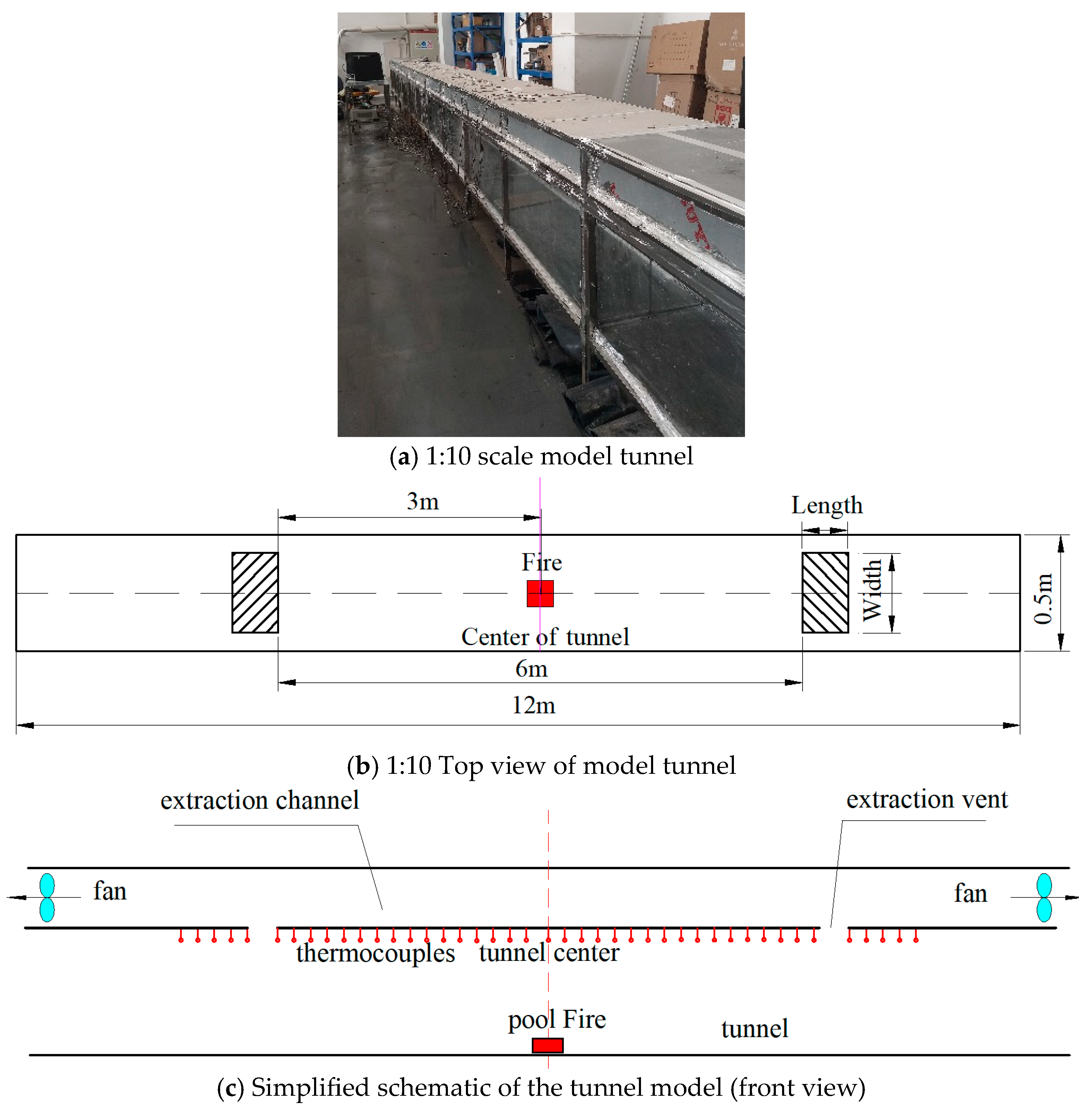
Figure 2a shows the physical diagram of the 1:10 tunnel model. Experiments were conducted in Chengdu (Approximately 100 kPa) and Xinduqiao (66.2 kPa), featuring an upper smoke exhaust channel (12 m × 0.5 m × 0.2 m) and a lower tunnel (12 m × 0.5 m × 0.5 m). Figure 2b illustrates that two smoke exhaust vents were symmetrically positioned along the tunnel centerline, 3 m from the tunnel center. The exhaust system was connected to fans via flexible hoses and PVC pipes. During the experiment, the exhaust rates of the two side fans were regulated to be consistent using valves and frequency converters, and measured by vortex flowmeters with an accuracy of 1.5%.

Temperature was measured with 1 mm Type K thermocouples (1.5 °C accuracy), placed 0.02 m below the ceiling at 0.1 m intervals (Figure 2c). Data were collected by an Agilent 34980A system produced by Keysight Technologies of the United States (Santa Rosa, CA, USA), with every 5 s and averaged over the stable period. Square n-heptane pool fires were used as heat sources: 2 cm high oil pans (2 cm above the floor) with side lengths of 6.5 cm, 7.4 cm, and 8.5 cm corresponded to heat release rates of 4.37 kW, 5.68 kW, and 7.5 kW, respectively [39].

3.2. FDS Numerical Simulation Model

Numerical simulation models were established using the Fire Dynamics Simulation (FDS). It has been widely applied in fire research, and FDS has been validated by extensive experiments [40,41,42].

3.2.1. Fire Source Setting

In numerical simulations, two fire source configuration methods were used. The fixed heat release rate method (fixed-HRR) directly specifies HRR, enabling rapid transition to stable combustion and saving computational resources for known HRR scenarios. The vaporization combustion of liquid fuel method determines HRR by modeling real pyrolysis processes, suitable for varying ambient pressures, as fuel heat release differs with pressure [43]. However, this approach demands substantial computational resources.

The fixed-HRR method was employed for numerical simulations under normal pressure (100 kPa), with HRR values of 5 MW, 10 MW, 20 MW, and 30 MW to balance efficiency and accuracy. CO yield (0.01) and smoke yield (0.008) followed FDS User Guide recommendations [44]. Under reduced atmospheric pressure, the vaporization combustion of liquid fuel method was used, first established with the exact dimensions of the scaled experimental setup. The fire source was n-heptane, consistent with the scaled experiment, using oil pans with side lengths of 6.5 cm, 7.4 cm, and 8.5 cm. Subsequently, full-scale models were constructed to simulate fire combustion and smoke movement. The fire sources were modeled as rectangles with four different side lengths (D = 1.15 m, 1.58 m, 2.24 m, and 2.72 m), corresponding to HRR values of 5 MW, 10 MW, 20 MW, and 30 MW under normal pressure (100 kPa) conditions.

3.2.2. Boundary Condition Setting

As shown in Figure 3, the two ends of the tunnel were set as “Open” boundary conditions to simulate the compensatory airflow induced by smoke extraction. The exhaust channel’s endpoint is “Exhaust”. The vent was defined as a “Hole”. The tunnel walls were assigned a “Concrete” boundary condition, with the ambient temperature at 20 °C. Four environmental pressures were considered: 100 kPa, 80 kPa, 60 kPa, and 40 kPa. The inclined tunnel model simulates the slope change by altering the direction of the gravity vector. This method has been applied in multiple inclined tunnel fire studies [11].

Thermocouples are set at intervals of 1 m and 0.2 m below the tunnel’s ceiling to measure the temperature (for the 1:10 scale model, setting at intervals of 0.1 m and 0.02 m below the tunnel’s ceiling).

3.2.3. Grid Sensitivity Analysis

To ensure the reliability of the simulation, it is necessary to determine a reasonable grid size, which can not only guarantee the accuracy of the calculation results but also save computing time. As shown in Figure 4, simulation calculations were carried out for four grid sizes of 0.25, 0.2, 0.15, and 0.1 m. It can be seen from the figure that with the gradual encryption of the grid, the temperature distribution gradually increases until the difference is minimal. In order to balance the calculation cost and accuracy, the grid size of 0.15 is a suitable choice (when it is a 1:10 scale model, the mesh size is 0.015 m).

3.2.4. Verification of Model Accuracy

As shown in Figure 5, it is a comparison diagram of the temperature distribution below the tunnel ceiling between the experiment under a specific working condition (the atmospheric pressure is 100 kPa, the ambient temperature is 20 °C, the fire source is located in the center of the tunnel, and the volumetric flow rate is 60 m³/h.) and the numerical calculation simulation model. As shown in the figure, temperature errors between experimental and numerical simulation results for various oil pan sizes are overall within 10%. This indicates the FDS model can accurately replicate tunnel vault temperature distribution, making it suitable for simulation data collection in follow-up multi-factor scenarios.

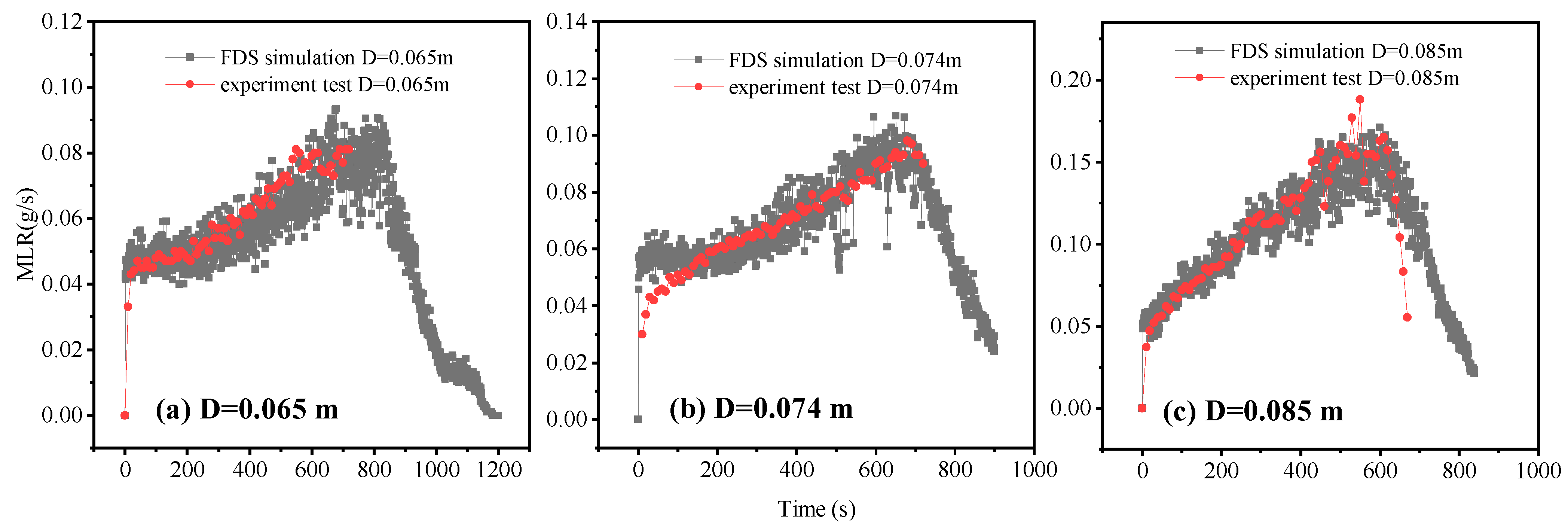
Figure 6 shows the comparison between the experimental results and the numerical simulation results of the change in fuel mass loss rate with the combustion time under three oil pan sizes at ambient pressure (66.2 kPa) in Xinduqiao area (the ambient temperature is 20 °C, the fire source is located in the center of the tunnel, and the volumetric flow rate is 60 m³/h). It can be seen that the simulation results are in good agreement with the experimental results, which verifies the reliability of the adopted grid size and the accuracy of the numerical calculation model.

3.3. Fire Scenarios

This study involves research on multiple models and various fire scenarios, and the details of the research conditions are sorted out in

Table 1. Summary of Test and Simulation Conditions.

No.	Series	Research Contents	Tunnel Size (H × W)	Fire Source Setting (HRR/kW, D/m)	P /kPa	Slope i
1–3	Normal pressure horizontal tunnel experiment	HRR, P	0.5 m × 0.5 m	HRR: 4.37/5.68/7.5 D: 0.065/0.074/0.085	100	0
3–6	Low-pressure horizontal tunnel experiment	HRR, P	0.5 m × 0.5 m	HRR: Obtained from experiments D: 0.065/0.074/0.085	66.2	0
7–18	Multi-pressure horizontal tunnel simulation	HRR, P	0.5 m × 0.5 m	HRR: Obtained from simulations D: 0.065/0.074/0.085	100/80 /60/40	0
19–34	Multi-pressure horizontal tunnel simulation	HRR, P	5 m × 5 m	HRR: Obtained from simulations D: 1.15/1.58/2.24/2.72	100/80 /60/40	0
35–50	Simulation of the Inclined Tunnel at H1	HRR, P, i, H	7 m × 5 m	HRR: 5000/10,000/20,000/30,000 D: 1.15/1.58/2.24/2.72	100	0/2%/ 4%/6%
51–62	Simulation of the Inclined Tunnel at H2	HRR, P, i, H	5 m × 5 m	HRR: 5000/10,000/20,000/30,000 D: 1.15/1.58/2.24/2.72	100	2%/4% /6%
63–70	Simulation of the Inclined Tunnel at H3	HRR, P, i, H	8 m × 5 m	HRR: 5000/10,000/20,000/30,000 D: 1.15/1.58/2.24/2.72	100	0/2%/ 4%/6%
71–78	Simulation of the Inclined Tunnel at H4	HRR, P, i, H	10 m × 5 m	HRR: 5000/10,000 D: 1.15/1.58	100	0/2%/ 4%/6%
79–82	Simulation of the Inclined Tunnel at H5	P, i, H	15 m × 5 m	HRR: 5000 D: 1.15	100	0/2%/ 4%/6%

. In addition, previous studies have shown that in the double-point smoke exhaust system, the smoke exhaust volume and the size of the smoke exhaust vent have little influence on the temperature of the tunnel roof [32]. Therefore, the full-scale model keeps the smoke exhaust volume at 3.5 m³/s, and the smoke exhaust volume in the 1:10 scaled-down model is 40 m³/h. The smoke exhaust outlet of the full-scale model is 2 m long and 4 m wide, and the size of the smoke exhaust outlet in the 1:10 scaled-down model is 0.2 m long and 0.4 m wide.

4. Establishment of Machine Learning Regression Prediction Models

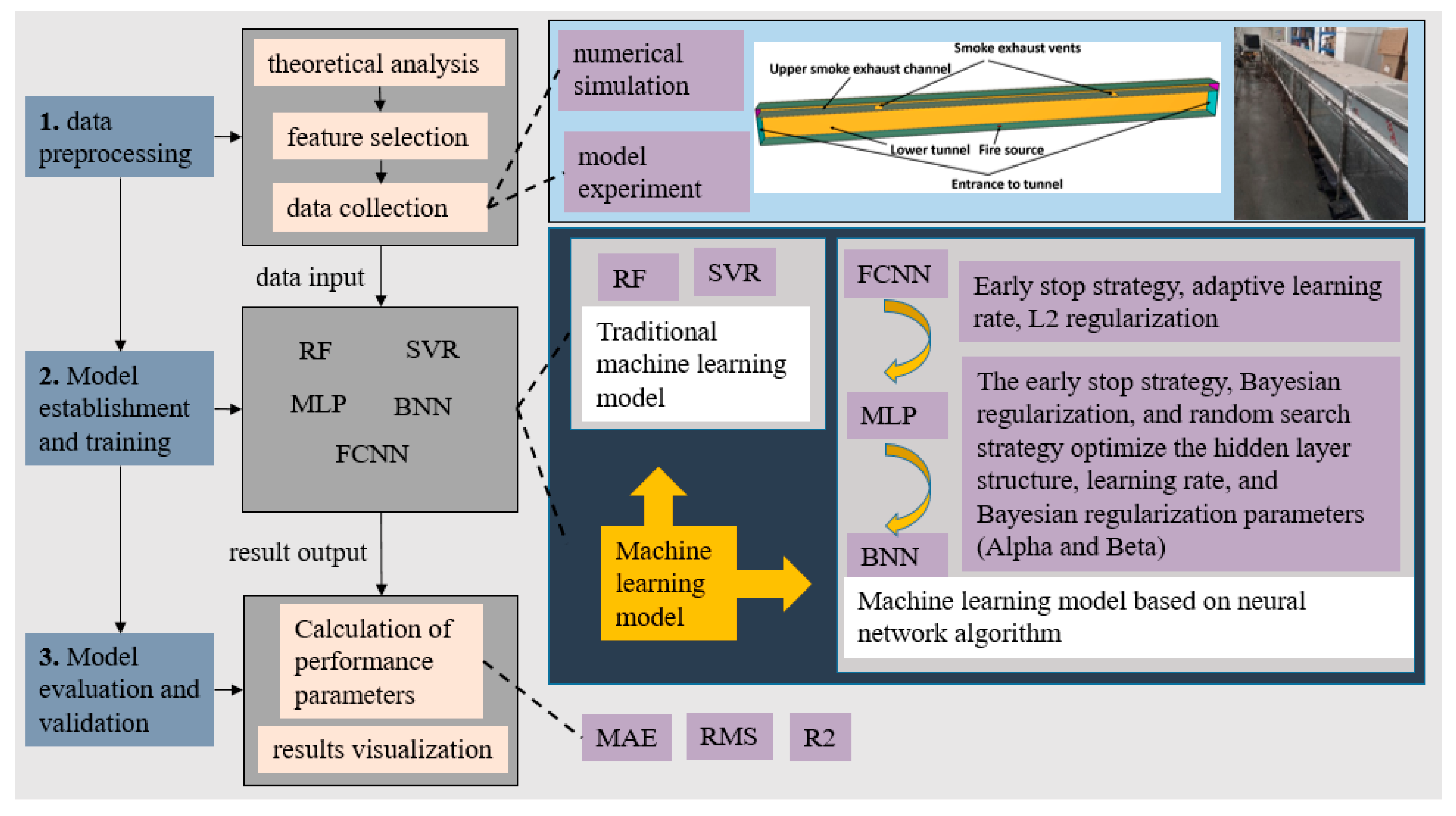
As shown in Figure 7, the machine learning-based regression prediction comprises three key steps: data preprocessing, model establishment and training, model evaluation, and validation.

4.1. Data Preprocessing

(1)

Feature selection

Data feature optimization is a core step in constructing machine learning models to enhance model performance. Rational feature engineering can effectively extract the essential attributes of data, strengthen data representation capabilities, and significantly improve the model’s prediction accuracy, robustness, and generalization ability. According to the theoretical derivation in Section 2, Equation (14) is obtained.

Since T₀ (≈20 °C, constant) does not vary, it was discarded. The model input variables were set as [Q*^2/3, (H_d/D)^−5/3, P, i], with the maximum excess temperature beneath the tunnel ceiling as the output variable.

(2)

Standardization processing

This paper uses the z-score standardization method to preprocess the input features and output labels, with the formula as follows:

$$X_{norm}={\displaystyle \frac{X_i-\mu }{\sigma }}$$

(15)

where X_i is the original data value (a feature value of the i-th sample), μ is the mean of all data points in the feature column, and σ is the standard deviation of all data points in the feature column.

(3)

Dataset partitioning

This study employed a random partitioning strategy for the 82 collected data samples, dividing the dataset into a training set (57 samples, 70%), a validation set (12 samples, 15%), and a test set (13 samples, 15%). All datasets are entirely independent. The training set serves model training, the validation set for performance verification (model selection and hyperparameter tuning), and the test set to assess the model’s final generalization ability. Random indices were generated using the randperm function to ensure random data partitioning, eliminating order bias that could affect model performance.

4.2. Model Establishment and Training

The matching degree between model complexity and data volume directly determines the prediction performance. This research falls under the category of regression prediction for structured small sample data. For such tasks, five models were selected and established for comparison: Firstly, two typical traditional machine learning models are constructed: Random Forest (RF) and Support Vector Regression (SVR). For more complex traditional machine learning models, such as XGBoost 2.1.4 and LightGBM 4.3.0, due to the complexity of their parameters and network settings, they are more suitable for samples with large data volumes. They are highly prone to overfitting when applied to small-sample data. Therefore, they are not selected in this paper. In addition, machine learning models based on neural network algorithms exhibit strong nonlinear mapping capabilities. The neural network models selected in this study primarily include the Fully Connected Neural Network (FCNN), Multilayer Perceptron (MLP), and Bayesian Neural Network (BNN).

Regarding deep learning models such as Convolutional Neural Network (CNN) and Transformer, the former is more suitable for processing high-dimensional data such as images, while the latter is primarily designed for specific scenarios such as time-series data. Moreover, both models are characterized by large parameter scales, which lead to difficulties in convergence when trained on small samples and thus fail to meet the stability requirements of small-sample scenarios. Hence, they are not included in the comparative analysis.

This study aims to analyze the applicability of the above five machine learning models to the engineering problems addressed herein. A detailed introduction to each model is provided as follows.

(1)

Random Forest (RF) model

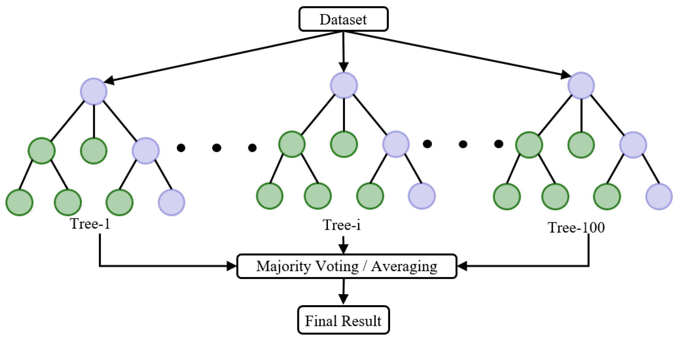
As shown in Figure 8, Random Forest, an ensemble learning method based on decision trees, constructs multiple decision trees and averages their prediction results. This model can handle nonlinear relationships and exhibits strong robustness against outliers and noise [45]. However, its computational complexity significantly increases with the growth of the number or depth of trees [46], making it more suitable for regression and classification tasks with medium-to-low-dimensional data.

The principle of its regression model is as follows:

$$\widehat{y}={\displaystyle \frac{1}{N}}{\displaystyle \sum _{i=1}^N{f}_i(x)}$$

(16)

where $\widehat{y}$ is the predicted value, f_i(x) is the predicted value of the i-th decision tree, and N is the number of decision trees.

In this study, a random forest regression model containing 100 decision trees was constructed using the TreeBagger function and trained via regression methods.

(2)

Support Vector Regression (SVR) model

Support Vector Regression (SVR) is a supervised learning model grounded in statistical learning theory [47], with its core principle residing in achieving precise prediction of continuous values by constructing an optimal hyperplane. As shown in Figure 9, SVR can handle nonlinear problems using kernel functions. By mapping data into a high-dimensional space through kernel functions, SVM is no longer limited by linear separation, thus enabling it to process more complex nonlinear data distributions and improving the model’s applicability and performance. SVR performs excellently in small sample learning scenarios. However, it has obvious limitations: its training complexity increases quadratically with the number of samples, leading to low training efficiency in large-scale data processing. Furthermore, the model is susceptible to selecting kernel functions and hyperparameters (such as penalty parameter C, threshold ε, kernel parameters, etc.), making the parameter tuning process complex and time-consuming.

The principle of its regression model is as follows:

$$\underset{w,b,\zeta ,{\zeta }^k}{\mathit{min}}{\displaystyle \frac{1}{2}}{‖w‖}^2+C{\displaystyle \sum _{i=1}^N({\zeta }_i+{\zeta }_i^k})$$

(17)

where w is the normal vector of the hyperplane, b is the hyperplane intercept, and are slack variables, C is the penalty parameter, and N is the number of samples.

The Gaussian kernel function can effectively address nonlinear relationships that are well-suited to complex tunnel temperature prediction demands. This study constructs an SVR model using the Gaussian kernel function. The penalty parameter BoxConstraint is set to 1, and the model is developed via the fitrsvm function in the 2024 (b) version of MATLAB.

(3)

Fully Connected Neural Network (FCNN) model

The Fully Connected Neural Network (FCNN) is the fundamental structure in neural networks, with neurons in each layer fully connected [48]. As illustrated in Figure 10, FCNN generally comprises an input layer, hidden layers, and an output layer, with neuron information transmitted between layers through weight matrices. The model calculates the loss function using the Back Propagation (BP) algorithm and updates weights via gradient descent. It is suitable for processing simple feature vector data and demonstrates nonlinear fitting capability and fast convergence on medium to small datasets.

The principle of its regression model is as follows:

$$\widehat{y}=f({\displaystyle \sum _{i=1}^N{w}_i{x}_i+b_i)}$$

(18)

where x_i represents the input signal, w_i is the input signal’s weight (reflecting the input’s importance to the neuron’s output), b is the bias term (adjusting the activation threshold of the neuron), and f is the activation function.

This study’s FCNN model employs a dual hidden layer architecture to improve the capture of complex nonlinear relationships. Using the newff function, a neural network with two hidden layers (8 and 4 neurons, respectively) was built. Training parameters were set: maximum iterations 1500, training target mean square error 1 × 10⁻⁷, learning rate 0.005, momentum factor 0.9. The tansig function was chosen for the hidden layers’ activation function, the purelin linear function for the output layer, and the Levenberg-Marquardt algorithm (trainlm) for training. Training halts when validation error fails to decrease for 30 consecutive iterations.

(4)

Multilayer Perceptron (MLP) model

The Multilayer Perceptron (MLP) [49,50] is a feedforward neural network composed of fully connected input, hidden, and output layers. MLP typically denotes a fully connected network with at least one hidden layer, while the fully connected layer can refer to single or multi-layer structures. When hidden layers exceed two, FCNN and MLP structures become nearly identical. The MLP model in this study is an optimized version of the FCNN model established in part (3), incorporating the following strategies:

• Increase the maximum number of iterations to 2000.
• Increase the early stopping patience value, and terminate training when the validation set error does not decrease 50 consecutive times to prevent overfitting.
• Adaptive learning rate: initial rate = 0.01, increase factor = 1.05, decrease factor = 0.7.
• L₂ regularization with weight decay = 0.001.

When the training data is insufficient, the model learns the noise or details of specific samples (such as outliers) in the data, leading to overfitting. L₂ regularization mitigates this by penalizing large weights, prompting the model to prioritize generalizable features. L₂ regularization adds the squared sum of weight parameters as a regularization term to the loss function to suppress overfitting. Its core principle is to force the model to learn simpler feature representations by punishing larger weight parameters. The total loss function after adding L₂ regularization is:

$$L=L_{data}+\lambda {\displaystyle \sum _{i=1}^N{w}_i^2}$$

(19)

(5)

Bayesian Neural Network (BNN) model

Bayesian Neural Network (BNN) integrates traditional fully connected neural networks (FCNN) with Bayesian regularization [51]. In this study, BNN is used as a further optimization model, with further enhancements achieved through the following critical steps:

• Parameter search: a stochastic search strategy optimizes the hidden layer architecture, learning rate, and Bayesian regularization parameters (α, β). Stochastic search is chosen for its superior efficiency in high-dimensional parameter spaces, which is particularly well-suited for multi-parameter optimization. The hyperparameter search space encompasses:

Hidden layer architectures: [6, 3], [8, 4], [10, 5];

Learning rates: 0.001, 0.005, 0.01;

Bayesian regularization parameter α (weight decay): 0.01, 0.1, 1, 10;

Bayesian regularization parameter β (noise precision): 0.01, 0.1, 1, 10.

After 30 stochastic search iterations, the optimal parameters (hidden layer [10, 5], learning rate = 0.001, α = 1.0, β = 1.0) are determined by minimizing validation set root mean square error (RMSE).

b.

BNN Training with Bayesian regularization: The BNN model is trained using the Bayesian regularization training algorithm (trainbr). In scenarios with limited data, manual tuning of the L₂ regularization parameter (λ) often leads to overfitting or underfitting. Bayesian regularization addresses this challenge by treating model parameters as random variables, introducing prior distributions, and maximizing the posterior probability to constrain model complexity automatically. The objective function is formulated as:

$$L=\beta L_{data}+\alpha {‖w‖}_2^2$$

(20)

where α and β are hyperparameters inferred automatically from data rather than manually set. This approach transforms regularization from an “empirical penalty” to a “systematic probabilistic inference,” making it highly effective for neural network optimization under data scarcity. By leveraging evidence maximization for automatic hyperparameter tuning, Bayesian regularization mitigates the high variance issues of cross-validation in small samples, outperforming traditional L₂ regularization in small-sample regression tasks.

4.3. Model Evaluation

Multiple evaluation indicators are simultaneously employed to evaluate each model’s predictive performance comprehensively. The coefficient of determination R² is used to measure the goodness of fit of the model to the data, with its calculation formula expressed as:

$$R^2=1-{\displaystyle \frac{{\displaystyle \sum _{i=1}^s{(y_{ei}-y_{pi})}^2}}{{\displaystyle \sum _{i=1}^s{(y_{ei}-{\overline{y}}_e)}^2}}}$$

(21)

Meanwhile, the root mean square error (RMSE) and the mean absolute error (MAE) measure the degree of deviation between the predicted and actual values. Their formulas are as follows:

$$RMSE=\sqrt{{\displaystyle \frac{1}{s}}{\displaystyle {\sum }_{i=1}^s(y_{ei}}-y_{pi}{)}^2}$$

(22)

$$MAE={\displaystyle \frac{1}{s}}{\displaystyle \sum _{i=1}^s\left|\left.\frac{y_{ei}-y_{pi}}{y_{ei}}\right|\right.}\times 100\%$$

(23)

where s is the number of samples, y_ei is the training target value of the i sample, and y_pi is the predicted value of each sample obtained by the model.

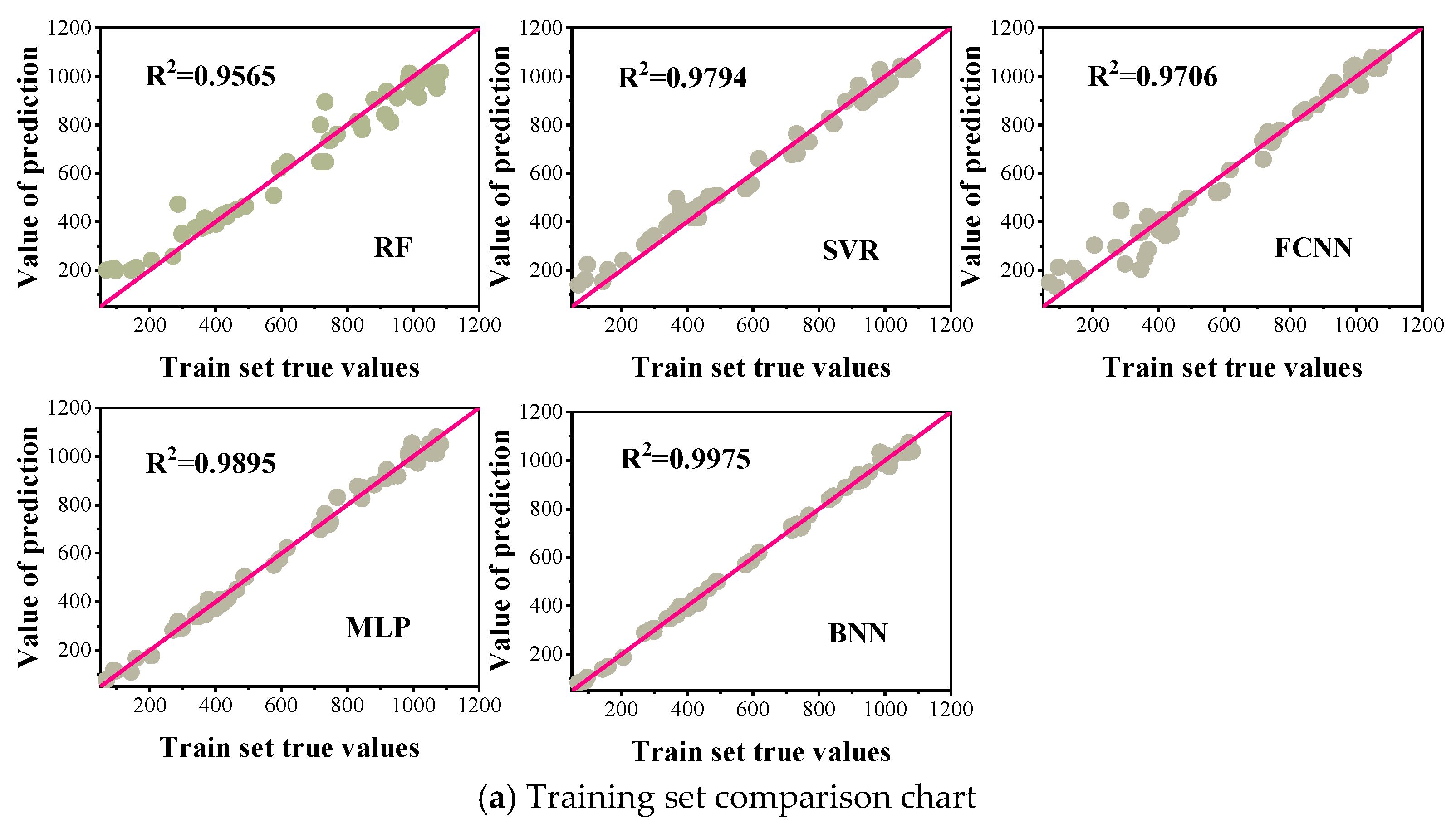
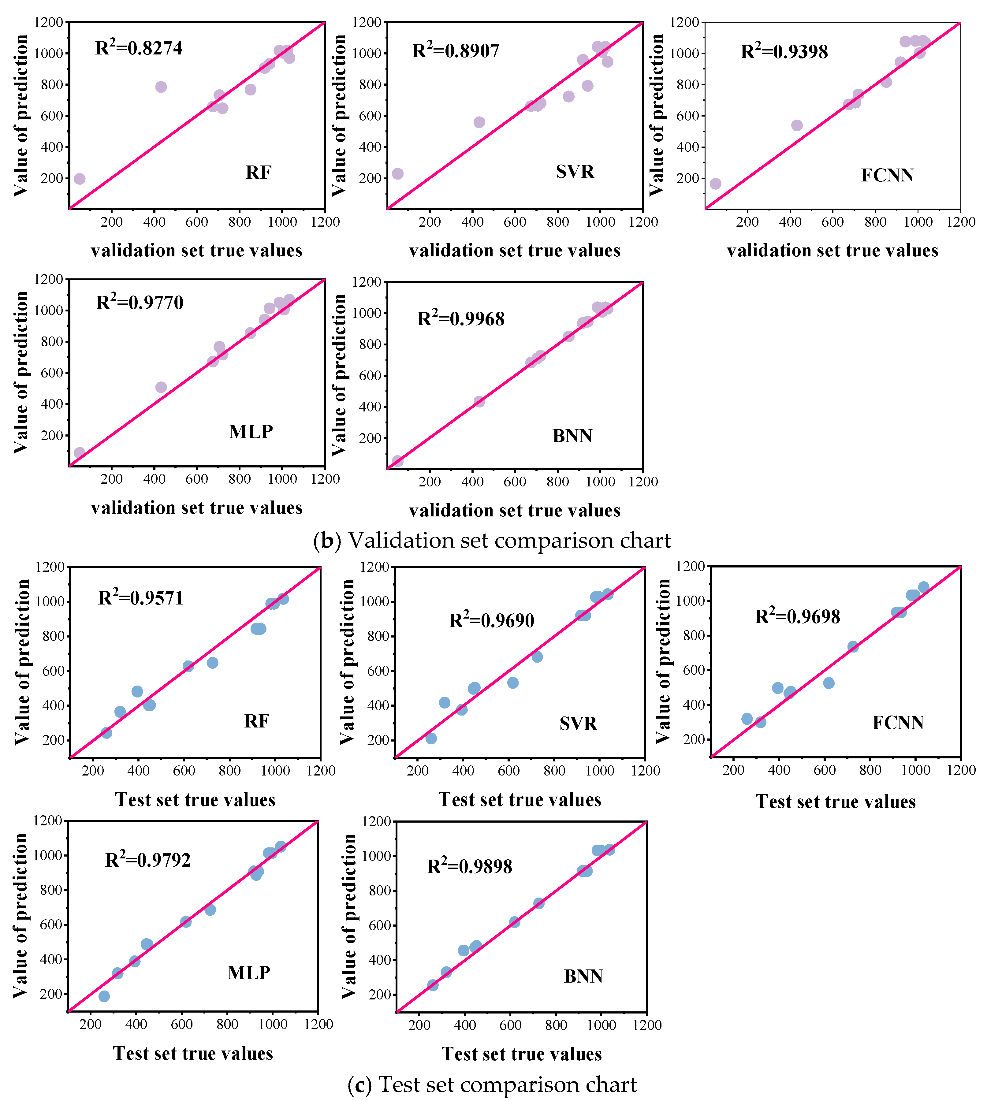
Figure 11 illustrates the predictive results of five models on the maximum excess temperature beneath the tunnel ceiling in tunnel fires across different datasets (training set, validation set, and test set). As shown in Figure 11, the Random Forest (RF) and Support Vector Regression (SVR) models exhibit relatively poor performance, with R² values below 0.90 in some cases, indicating weaker adaptability than neural network models in handling complex nonlinear relationships with multiple factors. The Fully Connected Neural Network (FCNN) generally aligns with actual values but has significant deviations in some samples. The R² values of the validation set and test set decrease obviously, reflecting that it is prone to overfitting and has insufficient generalization ability in small-sample scenarios. After optimization with strategies such as L₂ regularization and early stopping, the overall accuracy of the Multilayer Perceptron (MLP) is improved compared with that of the FCNN. The R² values on each dataset are all higher than 0.97, indicating the effectiveness of optimization strategies (early stopping, L₂ regularization, etc.) in improving the prediction performance of small samples.

Nevertheless, the performance of the MLP on the validation set is still lower than that on the training set, indicating that the model still has a certain degree of overfitting tendency. The Bayesian Neural Network (BNN) achieves the highest prediction accuracy, with R² values close to 1 (0.9975 for the training set, 0.9968 for the validation set, and 0.9898 for the test set). This fully demonstrates that by integrating random search hyperparameter optimization, Bayesian regularization, and early stopping strategies, the BNN accurately captures complex nonlinear relationships and demonstrates strong fitting and generalization abilities, making it more suitable for the small-sample complex linear regression prediction problem involved in this paper.

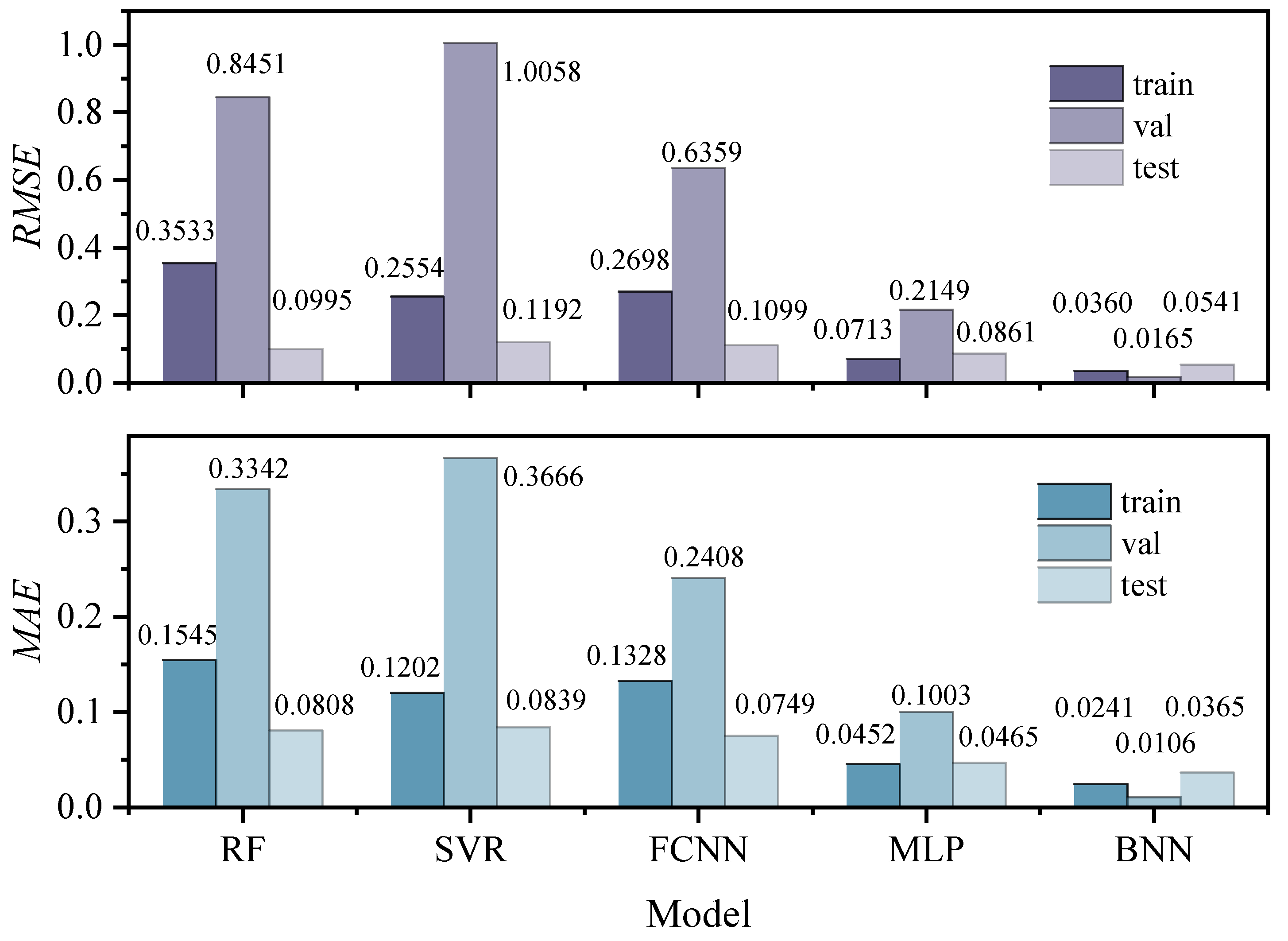
Figure 12 visually presents the MAE and RMSE of five models on the training, validation, and test sets. For RF and SVR, the test set’s MAE and RMSE are much higher than those of the training and validation sets, highlighting their generalization limitations under complex data. The FCNN has smaller increases in validation set MAE and RMSE compared to RF and SVR, thanks to its multi-layer nonlinear mapping. However, its fully connected structure’s parameter redundancy requires further optimization to boost generalization stability. The MAE and RMSE of the MLP model on the training and test sets are highly close, demonstrating the fitting stability of the model, which outperforms the FCNN.

Nevertheless, the increase in errors on the validation set reflects the limitation of the MLP in characterizing complex data distributions, making it difficult to adapt to the dynamic changes in data distributions fully. The MAE and RMSE of the BNN on each dataset are at extremely low levels with minimal differences. Optimization strategies such as Bayesian regularization effectively balance fitting and generalization, show strong robustness to changes in data distributions, and have significant advantages in small-sample and high-uncertainty scenarios.

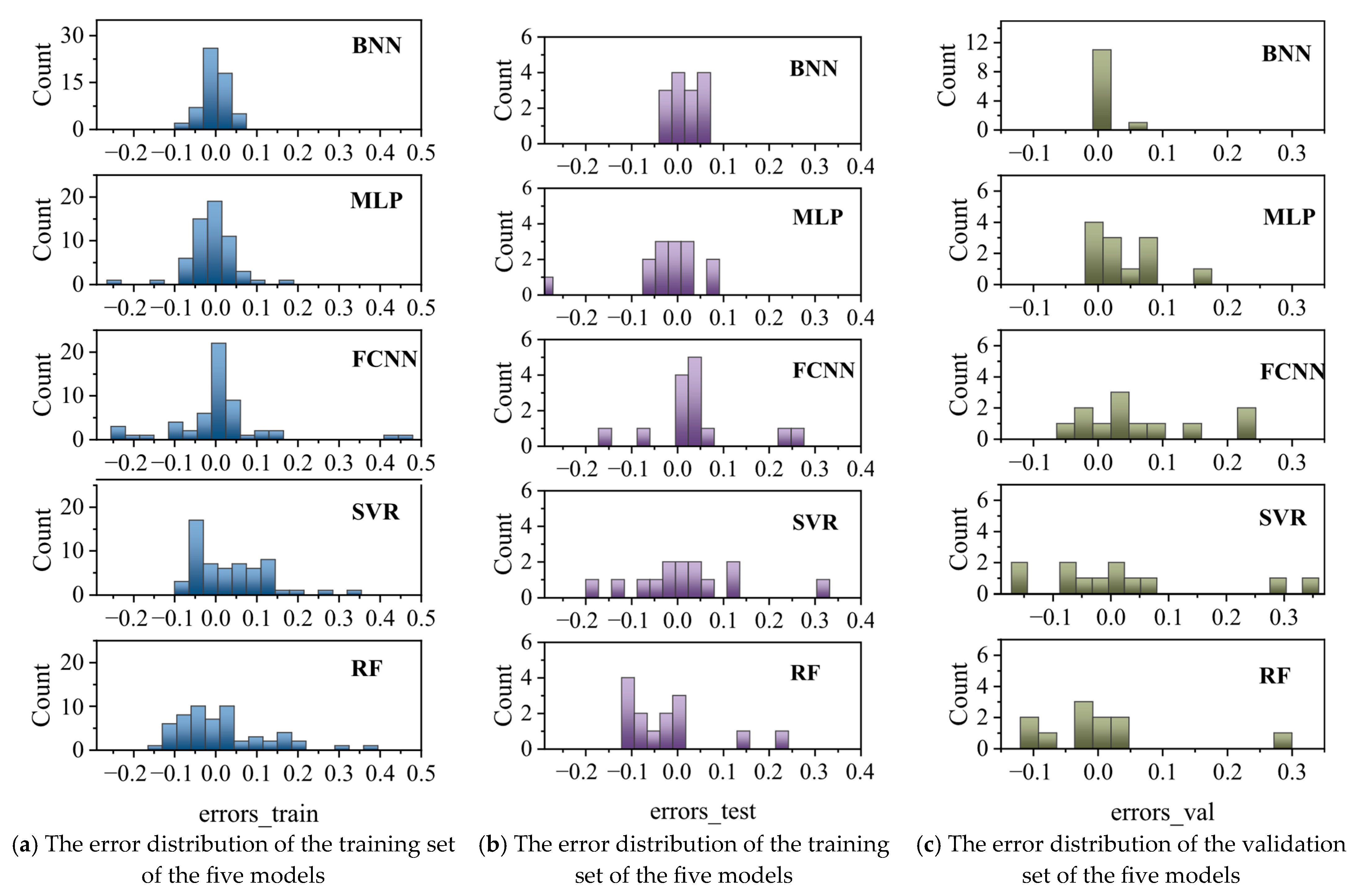
Figure 13 analyzes RF, SVR, FCNN, MLP, and BNN error distributions. The results show that BNN exhibits extremely high probability density peaks near the relative error 0 in the training, test, and validation sets, indicating concentrated errors and excellent accuracy. In contrast, RF, SVR, and FCNN exhibit discrete error distributions, with notable probability density values at −0.1, 0.25, and there is still a certain probability density distribution in the large error interval of 0.2–0.5, indicating large prediction fluctuations and limited nonlinear modeling ability for complex data. The error distribution of MLP is relatively balanced, but the overall concentration is weaker than that of BNN. These results highlight BNN’s superiority over the other models in prediction accuracy, stability, and generalization ability.

Figure 14 systematically evaluates five models in the form of a radar chart visualization. The comprehensive performance graph shows that BNN performs excellently in MAE, R², and RMSE throughout training, validation, and testing. Characterized by high fitting accuracy, strong generalization ability, and sufficient interpretation of data variation, BNN emerges as the optimal predictive model in this study. Although the MLP shows performance similar to that of BNN in the training set, its indicators in the validation and test sets are slightly inferior, indicating substantial room for improving the model’s generalization ability. In contrast, SVR, RF, and FCNN exhibit relatively poor overall performance. This study, through comprehensive evaluation with multiple indicators and comparative analysis, fully validates the remarkable advantages of BNN in related prediction tasks, providing an important theoretical basis and practical reference for model selection and optimization in similar problems.

Table 2. Model efficiency.

Model	RF	SVR	FCNN	MLP	BNN
Training time (s)	0.2288	0.1058	2.6382	2.6382	0.6458
Inference time (s)	0.0957	0.0364	0.0610	0.0151	0.0143

evaluates the computational efficiency of different models. Results show that the SVR model has the shortest training time in the training phase, while the MLP model takes the longest. Training is only performed during initial model deployment or dataset updates; no real-time repetition is needed, so it does not affect system real-time performance. All models achieve fast responses in the inference phase due to their small parameter scales and extremely low computational loads. The BNN model stands out particularly, with an inference time of only 0.0143 s, representing the best computational efficiency in this study.

4.4. Model Application and Expansion

After systematic comparison, the Bayesian Neural Network (BNN) prediction model developed in this study exhibits optimal performance. Nevertheless, its current application scope is clearly defined as follows:

(1)

Fire source: Single fire source;

(2)

Smoke exhaust layout: Tunnel with symmetric two-point smoke exhaust;

(3)

Environmental and structural parameters: Ambient pressure (40–100 kPa), tunnel slope (0–6%), rectangular cross-section, full-scale height (5–15 m), and width (5 m).

For scenarios beyond these boundaries, model optimization should focus on two aspects:

(1)

Incorporate scenario-specific physical features and refine the feature vector system to align model inputs with the new scenario’s physical mechanisms;

(2)

Supplement experimental/simulation data of out-of-bound scenarios to expand training sample coverage, thus mitigating increased generalization errors caused by data distribution shift.

Additionally, the current framework integrating physical feature dimensionality reduction and Binary Neural Network (BNN) models is expandable and applicable to predicting tunnel fire safety parameters (e.g., smoke movement, concentration characteristics) in other similar scenarios. Notably, while the core influencing factors of such parameters are similar and the framework is universal, specialized analysis of the physical coupling relationships between parameters for specific prediction targets remains necessary before practical application to ensure the model’s rationality and accuracy.

5. Conclusions

This study investigates rectangular tunnels with a single fire source and a two-point symmetric smoke exhaust system, tackling the regression prediction challenge of the maximum excess temperature beneath the tunnel ceiling under multiple factors. The scope involved includes strong and weak plume patterns, ambient pressure (40–100 kPa), tunnel slope (0–6%), full-scale tunnel height (5–15 m), and tunnel width (5 m). Five machine learning models are constructed and systematically compared to explore their performance in regression tasks with small-sample data. The main conclusions are as follows:

Through mathematical derivation and physical mechanism analysis, this study successfully screened and reconstructed feature vectors to accurately reflect the internal data laws. The optimization strategy significantly enhances data feature representational capability by removing redundant information and reinforcing key influencing factors.

Through comprehensive evaluation and comparative analysis of multiple indicators, this study thoroughly verifies the significant advantages of BNN in related prediction tasks. The Bayesian Neural Network (BNN) integrates optimization strategies (early stopping, regularization, and Bayesian inference) to mitigate overfitting in small-sample scenarios. Its Bayesian regularization, dual-hidden-layer design, and adaptive training enhance the performance and generalization of traditional feedforward networks, achieving optimal prediction accuracy for the maximum excess temperature beneath the tunnel ceiling. Random Forest (RF) employs ensemble learning via multi-decision tree voting, reducing overfitting risk but suffering from data distribution sensitivity and simple structure, leading to dispersed error distribution. Support Vector Regression (SVR) relies on kernel function mapping and margin maximization. However, it shows large errors in complex nonlinear scenarios or with poor kernel adaptability; its limited outlier robustness causes wide error intervals. Fully Connected Neural Network (FCNN) shows strong nonlinear fitting but tends to fall into local optima and is hypersensitive to hyperparameters, resulting in unstable error concentration. Multi-Layer Perceptron (MLP) improves performance through optimization methods but still lacks generalization capability.

The research clarifies effective models and strategies for small-sample prediction of the maximum excess temperature beneath the tunnel ceiling, promoting deep integration of machine learning with tunnel engineering. Due to limitations in personal capacity and resources, the study retains certain shortcomings. Future research will expand the range of incorporated influencing factors (e.g., tunnel shape diversity, environmental parameter variations) to enhance the model’s adaptability to complex scenarios. Additionally, it will refine the model from multiple dimensions: comparing more input feature dimensionality reduction methods, integrating physical mechanisms with data-driven models, using data augmentation to address small-sample issues, and incorporating uncertainty analysis to develop a more reliable and interpretable model.

References

1. Alarie, Y. Toxicity of fire smoke. Crit. Rev. Toxicol. 2002, 32, 259–289. [Google Scholar] [CrossRef]
2. Javadi, P.; Askari, M.; Vahedi, S.; GhafourianHesami, A.; Tizchang, A. Retrofit of RC buildings using vertical shear links and hybrid connections. Structures 2023, 48, 1788–1807. [Google Scholar] [CrossRef]
3. Islam, R.; Lattimer, B.Y. Understanding the Impact of Fuel on Surfactant Microstructure of Firefighting Foam. Fire Technol. 2024, 60, 3413–3441. [Google Scholar] [CrossRef]
4. Zhong, W.; Liu, L.; Han, N.; Gao, Z.; Zhao, J. Investigation on the maximum ceiling temperature of the weak plume impingement flow in tunnel fires under longitudinal ventilation. Tunn. Undergr. Space Technol. 2023, 131, 104821. [Google Scholar] [CrossRef]
5. Alpert, R.L. Calculation of Response Time of Ceiling-Mounted Fire Detectors. Fire Technol. 1972, 8, 181–195. [Google Scholar] [CrossRef]
6. Kurioka, H.; Oka, Y.; Satoh, H.; Sugawa, O. Fire properties in near field of square fire source with longitudinal ventilation in tunnels. Fire Saf. J. 2003, 38, 319–340. [Google Scholar] [CrossRef]
7. Hu, L.H.; Huo, R.; Peng, W.; Chow, W.K.; Yang, R.X. On the maximum smoke temperature under the ceiling in tunnel fires. Tunn. Undergr. Space Technol. 2006, 21, 650–655. [Google Scholar] [CrossRef]
8. Li, Y.Z.; Lei, B.; Ingason, H. The maximum temperature of buoyancy-driven smoke flow beneath the ceiling in tunnel fires. Fire Saf. J. 2011, 46, 204–210. [Google Scholar] [CrossRef]
9. Li, Y.Z.; Ingason, H. The maximum ceiling gas temperature in a large tunnel fire. Fire Saf. J. 2012, 48, 38–48. [Google Scholar] [CrossRef]
10. Liu, F.; Yu, L.X.; Weng, M.C.; Lu, X.L. Study on longitudinal temperature distribution of fire-induced ceiling flow in tunnels with different sectional coefficients. Tunn. Undergr. Space Technol. 2016, 54, 49–60. [Google Scholar] [CrossRef]
11. Ji, J.; Wang, Z.; Ding, L.; Yu, L.; Gao, Z.; Wan, H. Effects of ambient pressure on smoke movement and temperature distribution in inclined tunnel fires. Int. J. Therm. Sci. 2019, 145, 106006. [Google Scholar] [CrossRef]
12. Wang, Y. Study of Combustion Characteristics and Smoke Flow Control Method of Highway Tunnel in Very High Altitude Area. Ph.D. Thesis, Southwest Jiaotong University, Chengdu, China, 2019. [Google Scholar]
13. Wang, Q.; Wang, S.; Liu, H.; Shen, J.; Shang, F.; Shi, C.; Tang, F. Characterization of ceiling smoke temperature profile and maximum temperature rise induced by double fires in a natural ventilation tunnel. Tunn. Undergr. Space Technol. 2020, 96, 103233. [Google Scholar] [CrossRef]
14. He, K.; Li, Y.Z.; Ingason, H.; Shi, L.; Cheng, X. Experimental study on the maximum ceiling gas temperature driven by double fires in a tunnel with natural ventilation. Tunn. Undergr. Space Technol. 2024, 144, 105550. [Google Scholar] [CrossRef]
15. Beya, O.; Hittawe, M.; Sidibe, D.; Meriaudeau, F. Automatic detection and tracking of animal sperm cells in microscopy images. In Proceedings of the 2015 11th International Conference on Signal-Image Technology & Internet-Based Systems (SITIS), Bangkok, Thailand, 23–27 November 2015; pp. 155–159. [Google Scholar]
16. Hittawe, M.M.; Harrou, F.; Sun, Y.; Knio, O. Stacked Transformer Models for Enhanced Wind Speed Prediction in the Red Sea. In Proceedings of the 2024 IEEE 22nd International Conference on Industrial Informatics (INDIN), Beijing, China, 18–20 August 2024. [Google Scholar]
17. Wang, Z.; Zhang, T.; Wu, X.; Huang, X. Predicting transient building fire based on external smoke images and deep learning. J. Build. Eng. 2022, 47, 103823. [Google Scholar] [CrossRef]
18. Wu, X.; Zhang, X.; Huang, X.; Xiao, F.; Usmani, A. A real-time forecast of tunnel fire based on numerical database and artificial intelligence. Build. Simul. 2022, 15, 511–524. [Google Scholar] [CrossRef]
19. Cheng, J.; Yang, N.; Jiang, S.; Xiong, C. Real-time forecast of tunnel fire scenario and hazard based on external smoke images. Tunn. Undergr. Space Technol. 2025, 158, 106377. [Google Scholar] [CrossRef]
20. Yan, F.; Jiang, Y.; Chen, Y.; Xu, Z.-D. A data-driven model for tunnel fire scenario deduction based on optimized informer. Meas. Sci. Technol. 2025, 36, 108102. [Google Scholar] [CrossRef]
21. Sun, B.; Liu, X.; Xu, Z.-D.; Xu, D. Temperature data-driven fire source estimation algorithm of the underground pipe gallery. Int. J. Therm. Sci. 2022, 171, 107247. [Google Scholar] [CrossRef]
22. Guo, C.; Guo, Q.; Zhang, T.; Li, W.; Zhu, H.; Yan, Z. Study on real-time heat release rate inversion for dynamic reconstruction and visualization of tunnel fire scenarios. Tunn. Undergr. Space Technol. 2022, 122, 104333. [Google Scholar] [CrossRef]
23. Hu, P.; Peng, X.; Tang, F. Prediction of maximum ceiling temperature of rectangular fire against wall in longitudinally ventilation tunnels: Experimental analysis and machine learning modeling. Tunn. Undergr. Space Technol. 2023, 140, 105275. [Google Scholar] [CrossRef]
24. Liu, W.; Deng, L.; Li, H.; Li, X.; Shi, C.; Meng, N.; Tang, F. Experimental study and machine learning on the maximum temperature beneath tunnel ceiling induced by adjacent tandem fires in longitudinally ventilated tunnel. Int. J. Therm. Sci. 2023, 187, 108169. [Google Scholar] [CrossRef]
25. Li, M.; Jiang, Y.; Wu, Z.; Fan, R. Real-Time Prediction of Smoke Spread Affected by Multiple Factors in Subway Tunnel Using CAERES-DNN Model. Fire Technol. 2021, 57, 2025–2059. [Google Scholar] [CrossRef]
26. Sun, B.; Liu, X.; Xu, Z.-D.; Xu, D. BP neural network-based adaptive spatial-temporal data generation technology for predicting ceiling temperature in tunnel fire and full-scale experimental Verification. Fire Saf. J. 2022, 130, 103577. [Google Scholar] [CrossRef]
27. Sun, B.; Xu, Z.-D.; Zhou, H. A multiple back propagation neural network fusion algorithm for ceiling temperature prediction in tunnel fires. Eng. Struct. 2023, 280, 115601. [Google Scholar] [CrossRef]
28. Liu, X.; Sun, B.; Xu, Z.-D.; Liu, X.; Xu, D. Identification of Multiple Fire Sources in the Utility Tunnel Based on a Constrained Particle Swarm Optimization Algorithm. Fire Technol. 2022, 58, 2825–2845. [Google Scholar] [CrossRef]
29. Yang, W.; Chen, Z.; Zhao, H.; Chen, S.; Shi, C. Feature fusion method for rock mass classification prediction and interpretable analysis based on TBM operating and cutter wear data. Tunn. Undergr. Space Technol. 2025, 157, 106351. [Google Scholar] [CrossRef]
30. Zukoski, E.E.; Kubota, T.; Cetegen, B. Entrainment in Fire Plumes. Fire Saf. J. 1980, 107–121. [Google Scholar] [CrossRef]
31. Karlsson, B.; Quintiere, J.G. Enclosure Fire Dynamics; CRC Press: Boca Raton, FL, USA, 2022. [Google Scholar]
32. Zhao, P.; Yuan, Z.; Liang, C.; Yuan, Y.; Xie, Y.; Yu, N. Experimental investigation on ceiling temperature characteristics induced by weak and strong fire plumes in tunnel fires equipped with two-point extraction ventilation using smoke extraction channel. Tunn. Undergr. Space Technol. 2022, 124, 104487. [Google Scholar] [CrossRef]
33. Yan, G.; Wang, M.; Yu, L.; Tian, Y. Effects of ambient pressure on the critical velocity and back-layering length in longitudinal ventilated tunnel fire. Indoor Built Environ. 2020, 29, 1017–1027. [Google Scholar] [CrossRef]
34. Hu, L.; Wang, Q.; Delichatsios, M.; Tang, F.; Zhang, X.; Lu, S. Flame height and liftoff of turbulent buoyant jet diffusion flames in a reduced pressure atmosphere. Fuel 2013, 109, 234–240. [Google Scholar] [CrossRef]
35. Xu, T.; Tang, F.; Xu, X.; He, Q. Impacts of ambient pressure on the stability of smoke layers and maximum smoke temperature under ceiling in ventilated tunnels. Indoor Built Environ. 2023, 32, 85–97. [Google Scholar] [CrossRef]
36. Tan, T.; Yu, L.; Ding, L.; Gao, Z.; Ji, J. Numerical investigation on the effect of ambient pressure on mechanical smoke extraction efficiency in tunnel fires. Fire Saf. J. 2021, 120, 103136. [Google Scholar] [CrossRef]
37. Yang, Y.; Long, Z.; Cheng, H.; Chen, J.; Liu, C.; Zhong, M. Experimental and numerical study of smoke temperature distribution characteristics in a sloped tunnel. Sustain. Cities Soc. 2021, 73, 103091. [Google Scholar] [CrossRef]
38. Qu, H. Study on Natural Ventilation Smoke Gas Characteristics and Smoke Control of Sloped Tunnel Fires with Roof Openings. Master’s Thesis, Southwest Jiaotong University, Chengdu, China, 2022. [Google Scholar]
39. Zhao, P.; Yuan, Z.; Yu, N.; Liang, C. Effect of heat release rate and exhaust vent settings on the occurrence of plug-holing during tunnel fires with two-point extraction ventilation. Tunn. Undergr. Space Technol. 2020, 106, 103617. [Google Scholar] [CrossRef]
40. Yao, Y.; Wang, R.; Xia, Z.; Ren, F.; Zhao, J.; Zhu, H.; Cheng, X. Numerical study of the characteristics of smoke spread in tunnel fires during construction and method for improvement of smoke control. Case Stud. Therm. Eng. 2022, 34, 102043. [Google Scholar] [CrossRef]
41. Li, L.; Du, F.; Yang, Y.; Wei, L.; Huang, F.; Gao, Z.; Song, Y. Research on the smoke mass flow rate in one-dimensional spreading stage in tunnel with multiple fire sources. Case Stud. Therm. Eng. 2022, 31, 101801. [Google Scholar] [CrossRef]
42. Kazemipour, A.; Afshin, H.; Farhanieh, B. Numerical-Analytical Assessment of Fire and Ventilation Interaction in Longitudinally Ventilated Tunnels Using Jet Fans. Heat Transf. Eng. 2017, 38, 523–537. [Google Scholar] [CrossRef]
43. Liu, J.; He, Y.; Zhou, Z.; Yao, W.; Yuen, R.; Wang, J. The burning behaviors of pool fire flames under low pressure. Fire Mater. 2014, 40, 318–334. [Google Scholar] [CrossRef]
44. McGrattan, K.; Hostikka, S.; McDermott, R.; Floyd, J.; Vanella, M. Fire Dynamics Simulator User’s Guide, 6th ed.; NIST: Gaithersburg, MD, USA, 2018. [Google Scholar]
45. Ishwaran, H. Theory and Applications of Random Forests; Technical Report; University of Miami: Miami, FL, USA, 2011. [Google Scholar]
46. Rhodes, J.S.; Cutler, A.; Moon, K.R. Geometry- and Accuracy-Preserving Random Forest Proximities. IEEE Trans. Pattern Anal. Mach. Intell. 2023, 45, 10947–10959. [Google Scholar] [CrossRef]
47. Keshtegar, B.; Piri, J.; Abdullah, R.A.; Hasanipanah, M.; Sabri, M.M.S.; Le, B.N. Intelligent ground vibration prediction in surface mines using an efficient soft computing method based on field data. Front. Public Health 2023, 10, 1094771. [Google Scholar] [CrossRef]
48. Lewenstein, M.; Nowak, A. Fully connected neural networks with self-control of noise levels. Phys. Rev. Lett. 1989, 62, 225–228. [Google Scholar] [CrossRef] [PubMed]
49. Altunkaynak, A. Prediction of significant wave height using geno-multilayer perceptron. Ocean Eng. 2013, 58, 144–153. [Google Scholar] [CrossRef]
50. Thimm, G.; Fiesler, E. High-order and multilayer perceptron initialization. IEEE Trans. Neural Netw. 1997, 8, 349–359. [Google Scholar] [CrossRef] [PubMed]
51. Fila, R.J.J.; Attri, S.H.; Sharma, V. Mitigating Overfitting in Deep Learning: Insights from Bayesian Regularization. In Proceedings of the 2024 IEEE Region 10 Symposium (TENSYMP), New Delhi, India, 5–7 April 2024. [Google Scholar]
Figure 1. Simplified schematic of the tunnel model.
Buildings 15 03401 g001
Figure 2. Physical schematic diagram and layout schematic diagram of the tunnel model.
Buildings 15 03401 g002
Figure 3. Schematic diagram of the numerical simulation model.
Buildings 15 03401 g003
Figure 4. Grid sensitivity analysis.
Buildings 15 03401 g004
Figure 5. Comparison of the temperature distribution calculation results between the test and the simulation.
Buildings 15 03401 g005
Figure 6. Mass loss rate verification (66.2 kPa).
Buildings 15 03401 g006
Figure 7. The overall framework of the model construction.
Buildings 15 03401 g007
Figure 8. Schematic diagram of a decision tree in a random forest.
Buildings 15 03401 g008
Figure 9. The schematic diagram of Support Vector Regression (SVR), which solves nonlinear problems by using kernel functions.
Buildings 15 03401 g009
Figure 10. Schematic diagram of the Fully Connected Neural Network.
Buildings 15 03401 g010
Figure 11. Comparison chart of predicted values and actual values.
Buildings 15 03401 g011aBuildings 15 03401 g011b
Figure 12. Performance comparison of MAE and RMSE in different models.
Buildings 15 03401 g012
Figure 13. Schematic diagram of error distribution.
Buildings 15 03401 g013
Figure 14. Schematic diagram of the comprehensive evaluation radar.
Buildings 15 03401 g014