Joint Seismic Risk Assessment and Economic Loss Estimation of Coastal RC Frames Subjected to Combined Wind and Offshore Ground Motions

Abstract

The dynamic environment of coastal regions subjects infrastructure to multiple interacting natural hazards, with the simultaneous occurrence of windstorms and earthquakes posing a particularly critical challenge. Unlike inland hazards, these coastal threats frequently exhibit irregular statistical behavior and terrain-induced anomalies. This study proposes a novel probabilistic framework to assess compound hazard effects, advancing beyond traditional single-hazard analyses. By integrating maximum entropy theory with bivariate Copula models, a unified return period analysis is developed to capture the joint probability structure of seismic and wind events. The model is calibrated using long-term observational data collected from a representative coastal zone since 2000. For the PGA marginal distribution, our sixth-moment maximum-entropy model achieved an R² of 0.90, compared with 0.57 for a conventional GEV fit—reflecting a 58% increase in explained variance. Analysis shows the progressive evolution of damage from slight damaged through moderate damaged and severe damaged to collapse for an 18-story reinforced concrete frame structure, and shows that the combined effect of seismic and wind loads results in risk probabilities of aforementioned damage state of approximately 2 × 10⁻³, 6 × 10⁻⁴, 2 × 10⁻⁴, and 3 × 10⁻⁵, respectively, under a 0.4 g ground motion and a concurrent wind speed of 15 m/s. Furthermore, when both the uncertainty of loss ratios and structural parameters are incorporated, the standard deviation of the economic loss ratio reaches up to 0.015 in the transition region (PGA 0.2–0.4 g), highlighting considerable variability in economic loss assessment, whereas the mean economic loss ratio rapidly saturates above 0.8 with increasing PGA. These findings demonstrate that uncertainty in economic loss is most pronounced within the transition region, while remaining much lower outside this zone. Overall, this study provides a robust framework and quantitative basis for comprehensive risk assessment and resilient design of coastal infrastructure under compound wind and seismic hazards.

1. Introduction

Coastal structures, due to their unique geographic location and surrounding environment, face complex and severe threats from natural disasters. Coastal areas not only experience frequent seismic activity but are also often impacted by extreme weather events, such as strong winds, storms, and hurricanes. This combination of geographic and climatic conditions necessitates that coastal buildings address various complex environmental loads during both design and usage to ensure structural safety and reliability [1]. In today’s context of increasingly frequent and compounding natural hazards, robust multi-hazard risk modeling [2,3] and accurate economic loss estimation under uncertainty [4,5] are not only vital for understanding individual hazard impacts but are also critical for capturing the interdependencies and cascading effects that can arise during compound events. These analytical approaches allow for the development of quantitative resilience metrics, probabilistic risk assessments, and adaptive design strategies that collectively support the long-term functionality and reliability of coastal infrastructure systems [6,7].

Wind and earthquakes, as the two main natural disasters, have particularly significant impacts on coastal structures. Individual wind loads or seismic loads can cause severe damage, while their combined effects increase the likelihood of catastrophic structural failures. For instance, in 2021, several notable events illustrated the combined impact of wind and seismic hazards. On 18 April, Typhoon “Surigae” reached its peak intensity, and, shortly after, Hualien County in Taiwan experienced consecutive earthquakes of magnitude 5.6 and 6.1. On 13 June, before Typhoon “Chanhom” made landfall in Thanh Hoa Province, Vietnam, Yunnan Province in China was struck by two earthquakes with magnitudes greater than 5.0. Furthermore, from 4 to 6 August, Typhoon “Lu Bi” passed through China’s southeastern coastal regions, during which Taiwan experienced three earthquakes with magnitudes greater than 5.1. These instances highlight how coastal structures are at risk from both seismic and wind hazards occurring in close succession or simultaneously. Therefore, conducting in-depth research on the combined characteristics of wind and earthquakes, their return periods, and assessing the associated risks and expected economic losses for coastal structures is crucial for accurately evaluating the threats faced by these buildings under extreme conditions, and for formulating effective design and protective measures [8].

Reinforced concrete (RC) structures, known for their high strength, durability, and ease of construction, have seen widespread application in civil engineering in recent years. With continuous advancements in construction technology, RC structures are increasingly used in high-rise buildings, bridges, and various infrastructure projects. In recent years, with rapid developments in material science and structural analysis techniques, the design and construction methods of RC structures have been significantly improved. Especially under the combined effects of seismic, wind, and other multi-hazard loads, the performance of RC structures has been further enhanced, with innovative technologies increasingly applied to improve their disaster resistance and structural safety. This has made RC structures a crucial choice in modern construction, ideal for addressing complex engineering challenges [9,10,11,12,13]. Currently, the mechanisms and disaster processes affecting civil engineering structures under the dual impacts of seismic and strong wind forces have been a focal point of research within the civil engineering community, yielding systematic results. For instance, Vanessa [14] established a unified model for wind turbines under realistic sea conditions, using this model to evaluate the structural performance of offshore wind turbine structures—such as drift ratios, normalized base shear, and operational stability—under wind and seismic loads. Mensah [15] developed a model of offshore wind turbines considering aerodynamic and elastic characteristics, investigating the dynamic responses of this model under stochastic wind loads and recorded seismic events. Venanzi et al. [16,17] examined the dynamic responses of high-rise buildings under the combined effects of earthquakes and multiple hazards, proposing a comprehensive framework for lifetime loss assessment and life-cycle cost analysis under multi-hazard scenarios. Dogruel [18] suggested a multi-hazard optimization design and reinforcement method for building structures under combined seismic and wind loads based on lifetime cost indicators. The study by Athanasiou [19] proposes an improved multi-hazard design method for tall steel buildings in Eastern Canada, introducing a wind-related reduction factor (RW) to optimize structural performance under combined wind and earthquake effects, while verifying its impact on design response and collapse capacity. The work by Ciabatton [20] focuses on design trade-offs for tall buildings subjected to wind and earthquake loading, proposing a multi-hazard approach that integrates low-damage steel-timber systems and employs an Acceleration Displacement Response Spectrum (ADRS) to compare structural performance under these competing hazards, validated through case studies of 18- and 36-story buildings.

Existing research has pointed out that earthquakes and wind can mutually influence each other. For example, strong winds may trigger microseismic events and slow earthquakes, while typhoons can induce regular earthquakes, etc. For instance, Lin [21] found, through a study on the potential correlation between 102 typhoons passing near or traversing Taiwan from 1995 to 2011 and regular earthquakes, that the overall correlation was 63.75%. This correlation was particularly high after the 1999 Chi-Chi earthquake in Taiwan, where it increased from 16.67% to 78.21%. As a major earthquake, the Chi-Chi event significantly enhanced the previously low correlation between typhoons and seismic activity [22,23]. Additionally, earthquakes can also induce strong winds through mechanisms such as atmospheric temperature changes and electromagnetic wave anomalies. It is evident that there exists a potential nonlinear relationship between earthquakes and wind. Although considerable progress has been made in research on structural vulnerability under the joint influence of wind and earthquakes, there is a notable lack of studies focusing on the hazard analysis of these interactions, particularly regarding the patterns, probabilistic distribution characteristics, and joint return levels of multi-hazard events in coastal areas. This oversight not only results in an incomplete understanding of how coastal buildings withstand disasters but also hampers the development of effective optimization designs and disaster mitigation measures tailored to these structures [24,25]. By primarily focusing on vulnerability studies and neglecting the critical aspects of hazard analysis, the potential impacts of extreme weather and seismic events may be underestimated. This could lead to inadequate preparedness, increased economic losses, and compromised safety for occupants [26,27]. Therefore, conducting comprehensive risk assessments for coastal buildings that integrate real-world data and advanced statistical models is essential, as it would enhance the resilience of structures and inform better engineering practices and policy decisions, ultimately safeguarding communities against multi-hazard threats.

Moreover, in coastal regions, the seismic intensity characteristics in coastal areas can differ markedly from those inland, influenced by geological factors and proximity to fault lines [28,29]. Additionally, coastal winds often exhibit non-Gaussian behavior, which can lead to more extreme and unpredictable loading conditions compared to traditional Gaussian wind models. This non-Gaussian nature can result in higher peak wind forces and increased susceptibility to dynamic responses in structures, potentially exacerbating damage during extreme events [30,31,32,33]. Neglecting these distinct wind characteristics impedes a thorough evaluation of coastal buildings’ disaster resilience and limits the effectiveness of design strategies and mitigation measures. The lack of comprehensive risk analysis may lead to significant vulnerabilities, resulting in catastrophic consequences during storms or seismic events. Therefore, it is imperative to conduct robust risk assessments that incorporate actual data and sophisticated statistical models, enhancing the understanding of multi-hazard dynamics and improving the safety and resilience of coastal structures to better protect communities from potential disasters.

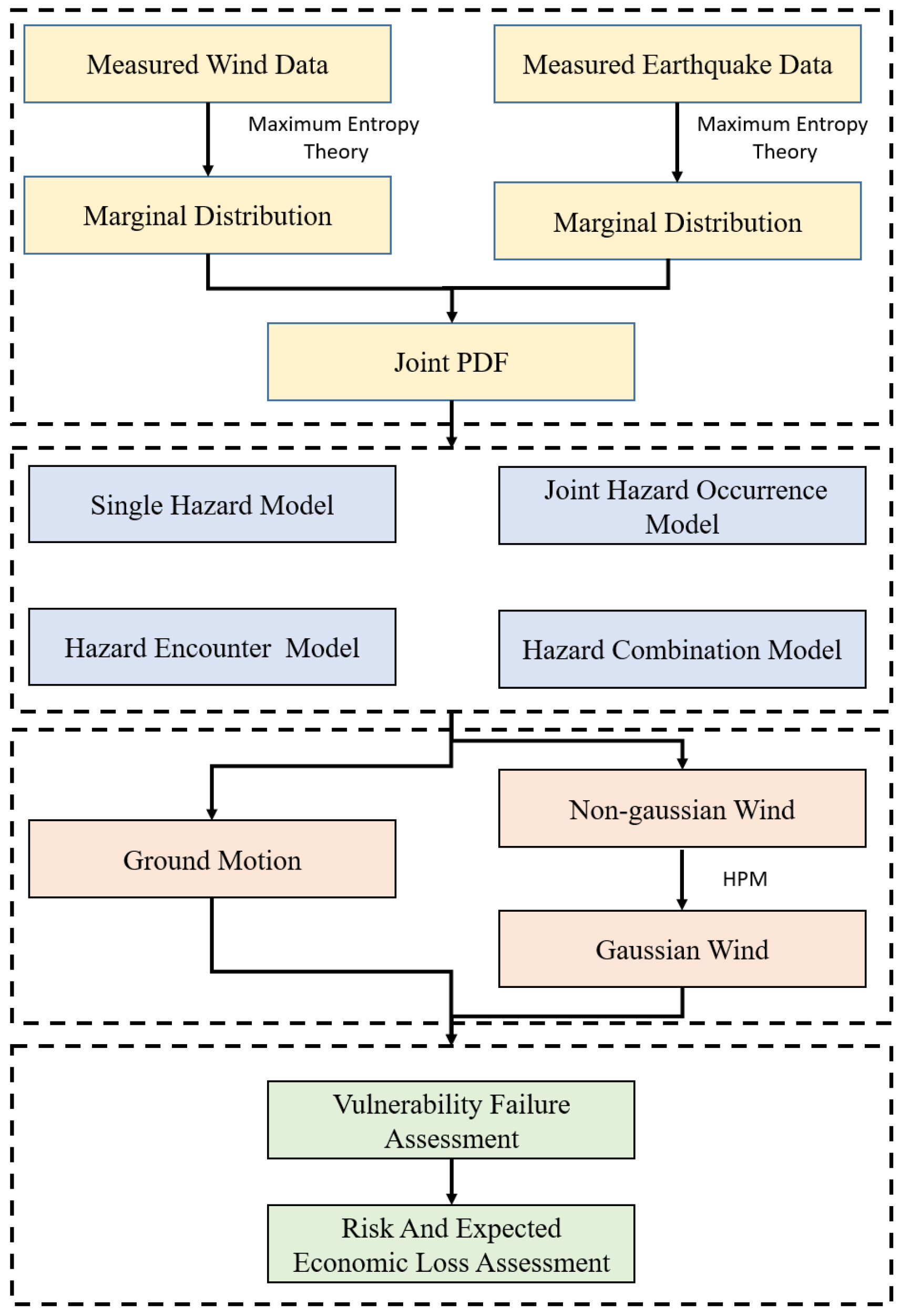
The core methodology of this study involves integrating various advanced statistical and theoretical models to comprehensively analyze the joint risk of wind and earthquakes. Specifically, this paper first collects observed offshore seismic motion data and time-averaged wind speed data from the KIK Seismic Station and the Japan Meteorological Agency since 2000, ensuring they share the same temporal and spatial characteristics. Next, peak acceleration and wind speed are constrained using the first six moments, and their marginal probability distributions are estimated through the maximum entropy model, ensuring precise capture of the data’s marginal characteristics. Subsequently, a joint probability distribution model of wind and earthquakes is constructed using Copula theory, revealing the dependence between the two. Finally, based on multi-hazard return period theory, four consistent hazard function models are employed to systematically analyze the joint exceedance probabilities and return periods of offshore earthquakes and strong winds under various scenarios. A coastal frame structure is selected as the engineering background, and its risk level and expected economic loss are assessed. In summary, this research systematically analyzes the risk characteristics of coastal buildings under the combined influence of wind and earthquakes, providing strong support for further structural safety research under multi-hazard conditions based on empirical data and statistical analysis. While our case study focuses on an 18-story coastal RC frame, the same probabilistic workflow—combining sixth-order moment marginal fitting, Copula-based joint hazard modeling, and multi-hazard fragility-loss surfaces—can be directly applied to other forms of structures, such as tunnel structures [34,35,36]. The flowchart of the study has been shown in Figure 1.

2. Source of Measured Data

The offshore seismic records used in this study were obtained from the KiK-Net strong motion database in Japan. This network comprises six closely spaced offshore stations dedicated to recording offshore seismic motion, as shown in

Table 1. Information on offshore station.

No.	Lat.	Long.	Depth (m)
KNG201	34.5956	139.9183	2197
KNG202	34.7396	139.8393	2339
KNG203	34.7983	139.6435	902
KNG204	34.8931	139.5711	933
KNG205	34.9413	139.4213	1486
KNG206	35.0966	139.3778	1130

. Due to the proximity of these six stations, they recorded a substantial amount of redundant data, which is not particularly meaningful for this study. Therefore, only the KNG206 station’s horizontal seismic records from January 2000 to December 2023, totaling 1574 measurements, were selected for analysis. Additionally, the raw data from the KIK database has not undergone any preprocessing, necessitating a series of treatments, including high-pass filtering, baseline correction, and energy clipping between the 1% and 99% thresholds, to ensure the accuracy of the research findings.

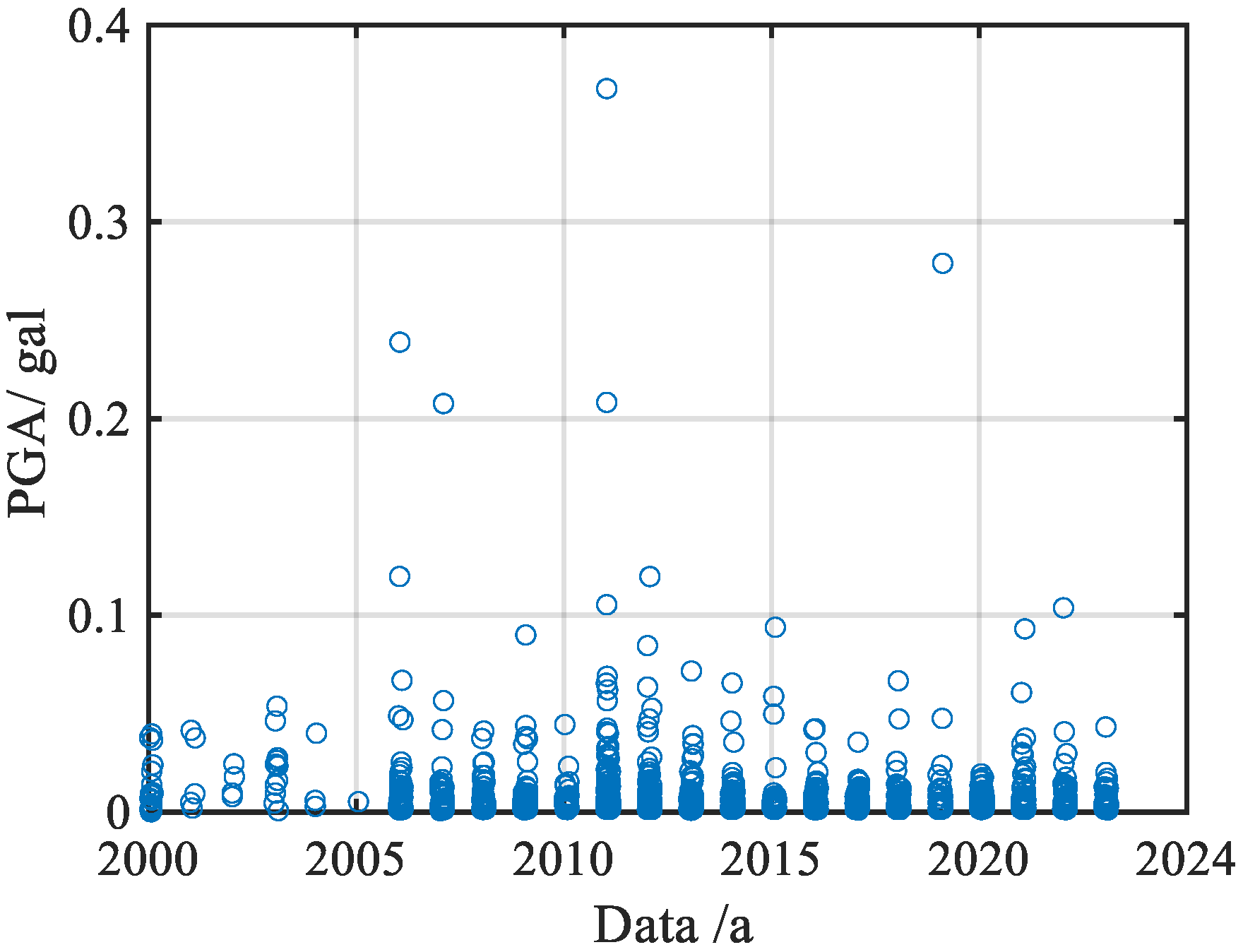
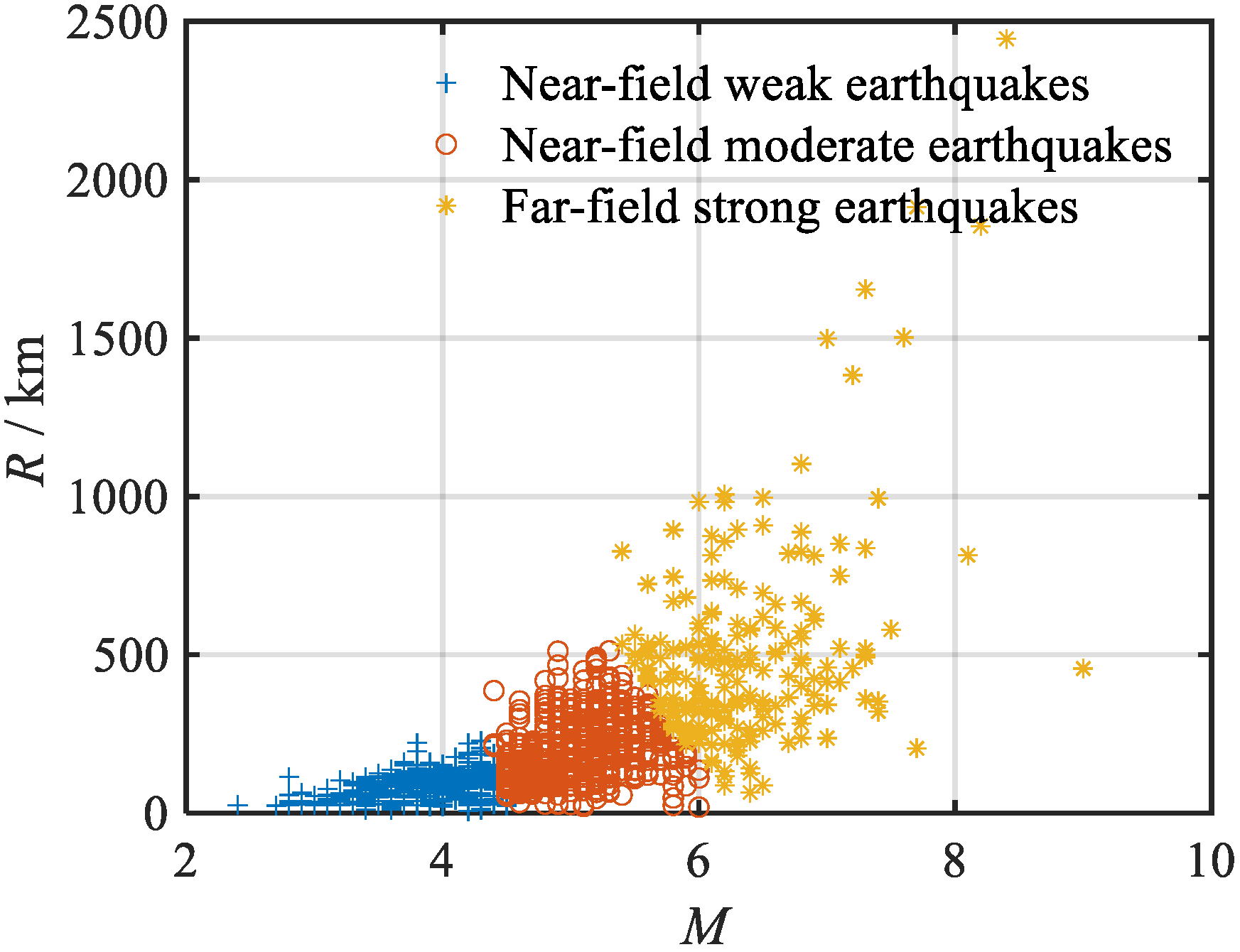
Furthermore, since the KiK-Net database does not provide site-specific information for the offshore stations, this study will utilize the K-means clustering method, based on the moment magnitude and epicentral distance (R), to categorize the offshore strong motion records into three groups: far-field large earthquakes, near-field moderate earthquakes, and near-field small earthquakes. There is no far-field small earthquake category due to the inability of small earthquakes to propagate over long distances. The clustering results are illustrated in Figure 2. It is evident that the grouping results from the clustering method bear similarities to the seismic classification outlined in the “Code for Seismic Design of Buildings” (GB 50011-2010) [37], with each category containing a comparable number of earthquakes, thus demonstrating the broad applicability of this study. The specific classification results are detailed in

Table 2. Corresponding number of cluster groups.

Clustering Group	Far-Field Large Earthquakes	Near-Field Moderate Earthquakes	Near-Field Small Earthquakes
Quantity	218	612	717

. Figure 3 presents a scatter plot of the occurrence time of offshore earthquakes and their peak accelerations. It is evident that while the intensity of offshore earthquakes is generally low, their frequency of occurrence is high, demonstrating significant sequential patterns.

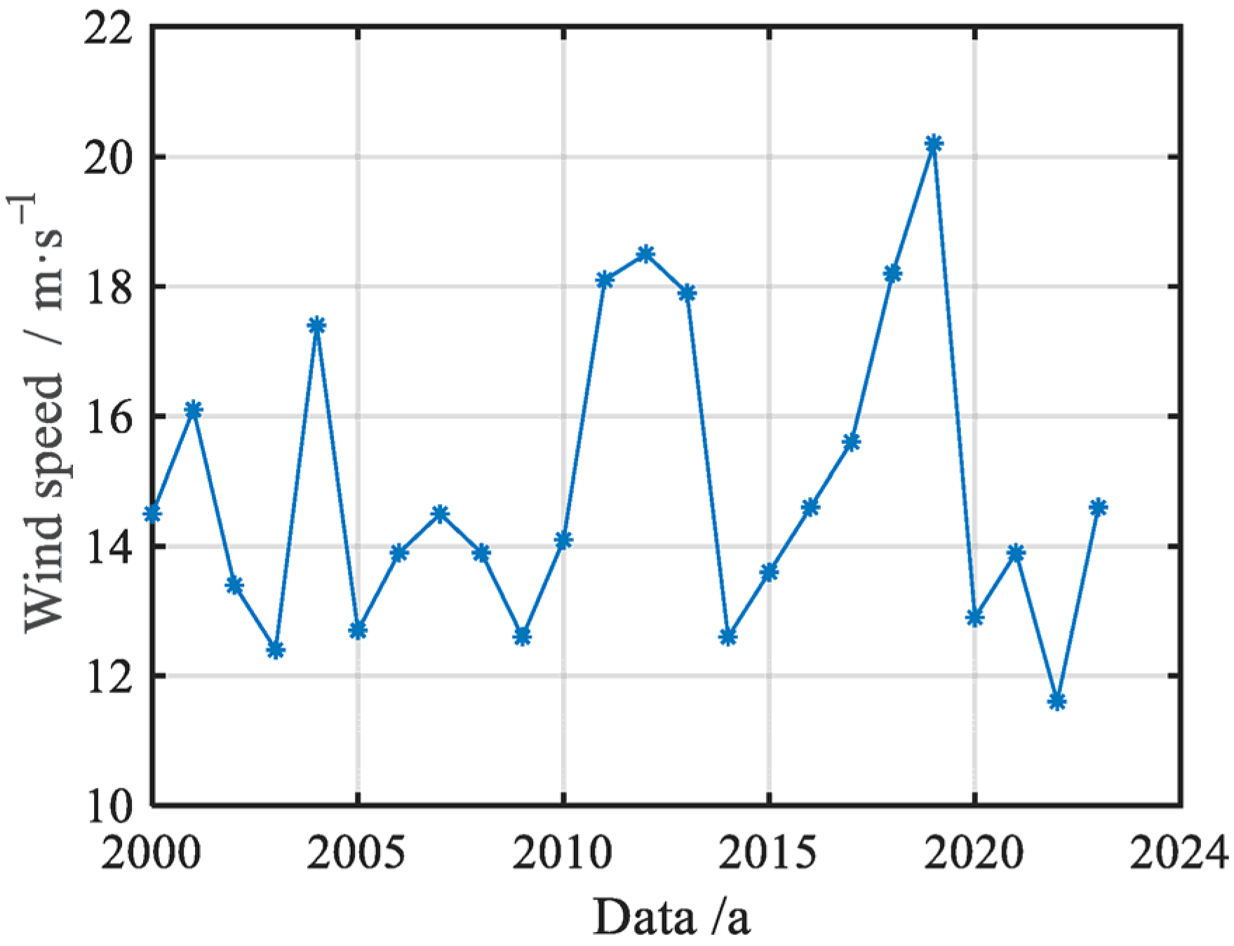
To ensure the reliability and consistency of the research results, this study obtained hourly average wind speed data from the Japan Meteorological Agency’s official website (https://www.data.jma.go.jp, accessed on 3 June 2024) that aligns with the location and time frame of the KNG206 station. This meteorological station is located in Yokohama, Kanagawa Prefecture, Japan, specifically at a latitude of 35.26 and a longitude of 139.39. Figure 4 presents a line chart of the annual extreme average wind speeds over 24 years. It is evident that the overall climate in this region is relatively stable, with few extreme events occurring. It is important to note that this study only selected wind speed data corresponding to the exact times of offshore earthquakes for analysis.

3. Hazard Analysis of Offshore Earthquakes and Strong Winds

3.1. Marginal Distribution Fitting Based on Maximum Entropy Theory

The maximum entropy theory, first proposed by scientist E.T. Jaynes in 1957, is a relatively young method for studying uncertainty. Entropy measures the degree of uncertainty or disorder in information. The main idea of maximum entropy theory is to calculate the probability distribution that maximizes entropy while adhering to known constraints derived from partially known information about the unknowns. For an unknown random variable X, its entropy can be defined as follows [38]:

$$E=-{\displaystyle {\int }_{-\infty }^{\infty }f(x)\log [f(x)]\mathrm{d}x}$$

(1)

where $f(x)$ indicates the probability density function of variable X, the maximization condition of its entropy is as follows:

$${\displaystyle {\int }_{-\infty }^{\infty }f(x)\mathrm{d}x}=1$$

(2)

$${\displaystyle {\int }_{-\infty }^{\infty }{u}_j(x)f(x)\mathrm{d}x}=r_j$$

(3)

where $j=1,2,\dots ,m$, $u_j(x)$ is the j-th function about the variable X. $r_j$ is a known constant, which is usually defined as the j-th moment of variable X. Based on the constraints from Equations (2) and (3), the Lagrange multiplier ${\lambda }_j$ is introduced to construct the functional G, defined as follows [38,39]:

$$G=E+({\lambda }_0+1)[{\displaystyle {\int }_{-\infty }^{\infty }f(x)\mathrm{d}x}-1]+{\displaystyle \sum _{j=1}^m{\lambda }_j[{\displaystyle {\int }_{-\infty }^{\infty }{u}_j(x)f(x)\mathrm{d}x}-r_j]}$$

(4)

By taking partial differentiation of $f(x)$ and maximizing G, the general solution of $f(x)$ can be obtained as follows:

$$f(x)=\exp [{\lambda }_0+{\displaystyle \sum _{j=1}^m{\lambda }_j{u}_j(x)}]$$

(5)

Therefore, by solving $u_j(x)$, a probability distribution model based on maximum entropy theory can be obtained. In this article, the constraint conditions consist of the first six moments of the random variable X, namely:

$${\displaystyle {\int }_{-\infty }^{\infty }f(x)\mathrm{d}x}=1$$

(6)

$${\displaystyle {\int }_{-\infty }^{\infty }{x}^{j}f(x)\mathrm{d}x}=M_j$$

(7)

$M_j$ is the corresponding j-th moment.

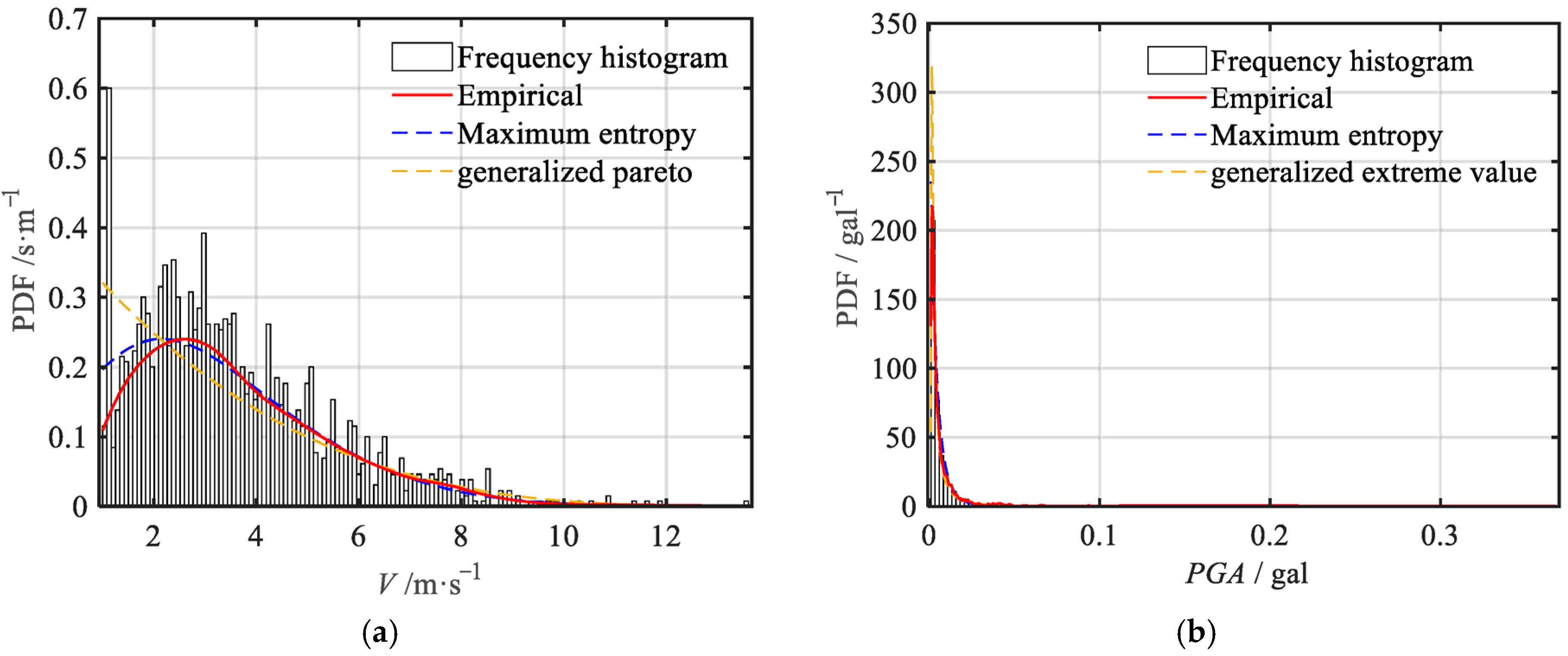
The first six moments of the PGA of offshore ground motion and simultaneous wind speed data are shown in

Table 3. The 1st to 6th moment of peak ground acceleration.

Intensity Parameter	Order
	1	2	3	4	5	6
Average wind speed	3.56	16.24	90.32	588	4362	36,045
PGA	$8\times {10}^{-3}$	$4.1\times {10}^{-4}$	$7.7\times {10}^{-5}$	$2.1\times {10}^{-5}$	$6.51\times {10}^{-6}$	$2.13\times {10}^{-6}$

. Furthermore, by substituting it as a constraint condition into Equations (5) and (7), the nonlinear equation system was solved, and the parameters were determined. The final results are shown in

Table 4. The 1st to 6th moment of mean wind speed.

Intensity Parameter	Order
	0	1	2	3	4	5	6
Average wind speed	−0.91	−4.66	30.64	−37.65	−1.49	61.32	−43.04
PGA	−4.45	99.69	−482.44	929.14	−400.97	−543.08	407.82

. Subsequently, in order to demonstrate the correctness of the maximum entropy model, the empirical kernel density function of the data was used as the target value to compare the results of the maximum entropy method and maximum likelihood estimation in Figure 5. Among them, the alternative probability models for maximum likelihood estimation include 17 probability models such as generalized extreme value distribution, Gumbel distribution, Weibull distribution, gamma distribution, etc., which shown in

Table 5. The fitting degrees of probability models of V.

Probability Model	BIC
Maximum Entropy	5830.41
Generalized Pareto	5902.75
Birnbaumsaunders	5952.58
Inverse Gaussian	5960.01
Lognormal	5970.19
Gamma	5981.71
Generalized Extreme Value	6006.470
Loglogistic	6040.43
Nakagami	6073.60
Rayleigh	6074.55
Rician	6081.90
Logistic	6316.77
Tlocationscale	6319.69
Normal	6361.06
Exponential	7033.84
Weibull	7136.94
Beta	7263.96
Tlocationscale	9963.6

and

Table 6. The fitting degrees of probability models of PGA.

Probability Model	BIC
Maximum Entropy	−13,085.23
Generalized Extreme Value	−13,075.64
Generalized Pareto	−12,966.33
Inverse Gaussian	−12,721.70
Loglogistic	−12,671.27
Lognormal	−12,646.40
Birnbaumsaunders	−12,481.49
Tlocationscale	−11,876.30
Gamma	−11,828.72
Exponential	−11,821.46
Beta	−11,772.99
Nakagami	−10,813.81
Logistic	−9927.24
Normal	−7900.65
Rayleigh	−6170.46
Rician	−6163.11
Extreme Value	−5936.23
Weibull	−5536.97

[40]. Intuitively speaking, the result of maximum entropy estimation is closer to the empirical mode function. Furthermore, taking peak acceleration as an example, the determination coefficients of the two methods were calculated to be 0.90 and 0.57, respectively. Therefore, it can be proven that the fitting effect of maximum entropy theory is significantly better than that of maximum likelihood estimation.

To evaluate the superiority of the maximum entropy model in modeling seismic parameters, Table 1 and Table 2 present a comparison of BIC values for different probabilistic models of wind speed (V) and peak ground acceleration (PGA), respectively. The results indicate that the maximum entropy model consistently yields the lowest BIC values, demonstrating its superior fitting performance compared to other models.

3.2. Hazard Analysis

Basic Theory of Recurrence Interval

In the engineering field, the recurrence interval is commonly used to characterize the frequency of occurrence of disaster parameters. For any type of disaster-causing parameter, its cumulative distribution function can be expressed as follows:

$$F(x)=\mathrm{Pr}[X\le x]$$

(8)

It is not difficult to obtain its probability of surpassing, as follows:

$$F^{\prime }(x)=\mathrm{Pr}[X>x]=1-F(x)$$

(9)

To this end, the recurrence interval of the disaster is the reciprocal of the probability of exceedance:

$$T(x)={\displaystyle \frac{1}{1-F(x)}}$$

(10)

Similarly, for multiple disasters, their joint recurrence interval can be defined in the following form:

$$T(x,y)={\displaystyle \frac{1}{P(x,y)}}$$

(11)

Among these, $P(x,y)$ is a consistent hazard function model of different types, which is related to the edge cumulative distribution functions $F(x)$, $F(y)$, and joint probability distribution function (JPDF) $F(x,y)$ of the random variables X and Y.

According to Sklar’s connection function theory, the FPDF $F(x,y)$ of random variables X and Y can be represented by the Copula function, i.e., [41]:

$$F(x,y)=C[F(x),F(y)]$$

(12)

Among these, $C(u_1,u_2)$ is the Copula joint cumulative distribution function (JCDF), which is the marginal cumulative distribution function of the random variables X and Y. Furthermore, four different consistent hazard function models are considered in this paper, which are the single model, co-occurrence model, encounter model, and combination model. Their definitions are as follows:

(1)

A single model represents the probability that at least one of the variables exceeds a certain threshold. It can be expressed probabilistically as follows:

$$P_1(x,y)=\mathrm{Pr}(X>x\cup Y>y)=1-F(x,y)$$

(13)

(2)

The co-occurrence model represents the probability of two variables simultaneously exceeding a threshold. It can be expressed probabilistically as follows:

$$P_2(x,y)=\mathrm{Pr}(X>x\cap Y>y)=1+F(x,y)-F(x)-F(y)$$

(14)

(3)

The encounter model represents the probability that when one variable exceeds a certain threshold, the other variable also exceeds the corresponding threshold. It can be expressed probabilistically as follows:

$$P_3(x,y)=\mathrm{Pr}(\left.X>x\right|Y>y)={\displaystyle \frac{1+F(x,y)-F(x)-F(y)}{1-F(y)}}$$

(15)

(4)

The combination model represents the probability that one variable does not exceed a certain threshold while the other variable exceeds the corresponding threshold. It can be expressed probabilistically as follows:

$$P_4(x,y)=\mathrm{Pr}(\left.X>x\right|Y<y)={\displaystyle \frac{F(y)-F(x,y)}{F(y)}}$$

(16)

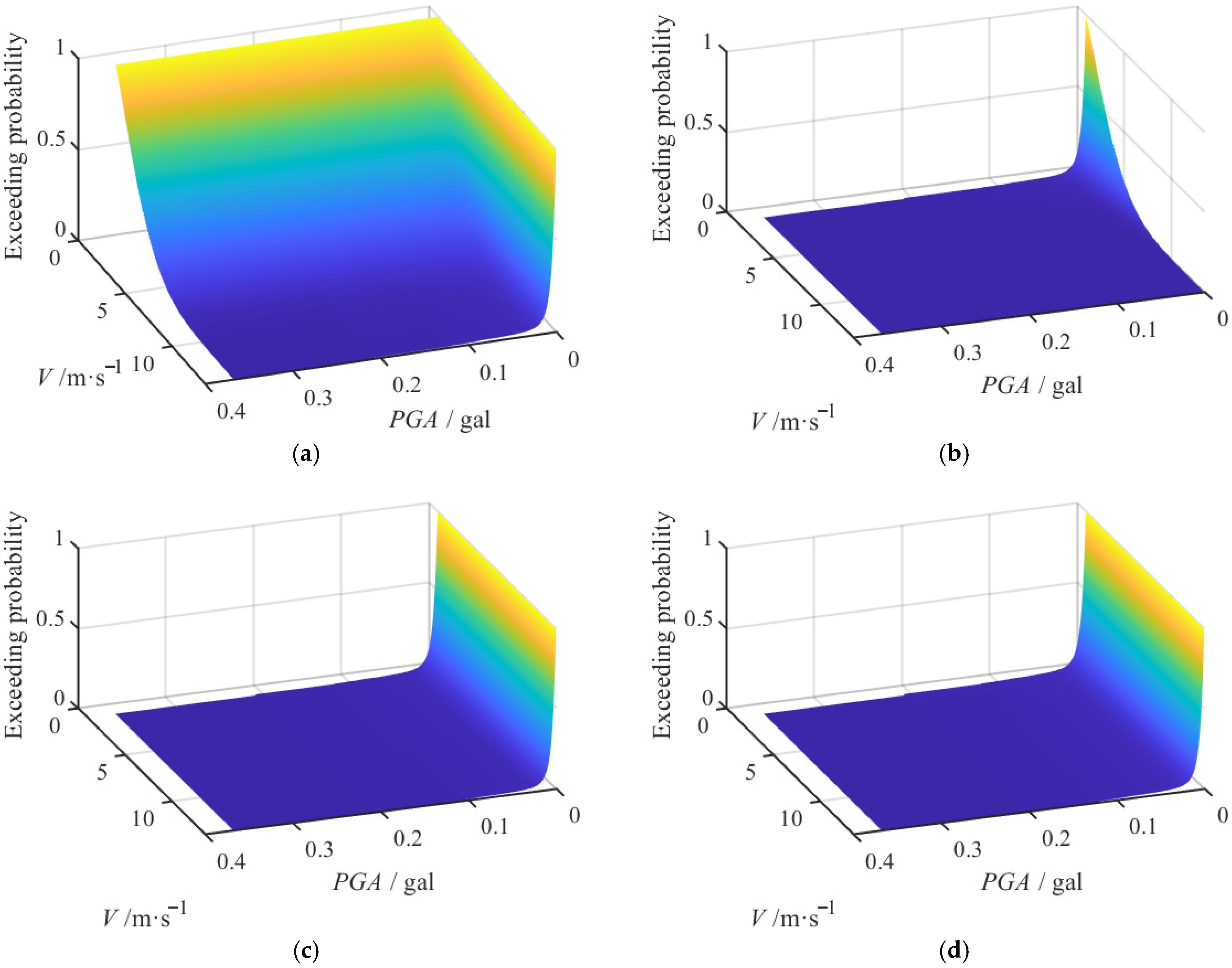
To further analyze the joint hazard of offshore ground motion and strong winds, let X represent the PGA of offshore ground motion and Y represent the average wind speed of strong winds. In this study, we utilize maximum likelihood estimation and the Bayesian Information Criterion BIC to select the optimal Copula function from five types of Copulas, including the Gaussian Copula and T Copula from the elliptical family, as well as Clayton, Plackett, and symmetric Clayton-type Copulas [42]. Ultimately, the selected optimal Copula function is the Gaussian Copula, with a corresponding Copula parameter of −0.028. Based on Equations (13)–(16), the calculated joint hazard function is illustrated in Figure 6. Subsequently,

Table 7. Return periods corresponding to different consistent hazard function models.

PGA (gal)	Return Period (a)	Average Wind Speed (m/s)	Return Period (a)	Return Period (a)
				Single Model	Co-Occurrence Model	Encounter Model	Combination Model
0.10	88	5	4.5	4.5	456.0	98.2	86.1
		10	150.8	55.9	16,626.3	110.2	88.3
		15	550.7	76.3	63,447.2	115.2	88.4
0.20	137	5	4.5	4.5	715.8	154.1	134.1
		10	150.8	72.2	26,332.7	174.6	137.7
		15	550.7	110.4	101,471.1	184.2	137.9
0.30	1984	5	4.5	4.6	10,666.7	2296.5	1913.8
		10	150.8	140.2	453,965.2	3009.6	1980.5
		15	550.7	431.2	2,751,821.5	4996.1	1982.8
0.40	2190	5	4.5	4.6	11,785.9	2537.5	2111.0
		10	150.8	141.2	509,067.1	3374.9	2185.1
		15	550.7	440.2	3,327,175.9	6040.6	2187.7

presents the recurrence periods of four joint hazard models under different peak ground acceleration and wind speed conditions, leading to the following conclusions:

(1)

The recurrence period of the single model is shorter than that of the individual hazards of underwater earthquakes and strong winds. For instance, when the peak ground acceleration and wind speed are 0.2 gal and 15 m/s, the corresponding recurrence periods for individual hazards are 137 years and 550 years, respectively, while the recurrence period for the single model is 110 years. This indicates that within a 110-year period, at least one occurrence of either a 0.2 gal underwater earthquake or a 15 m/s strong wind is expected.

(2)

The recurrence period for the joint occurrence model is significantly higher than that of the individual hazards. For example, when the peak ground acceleration and wind speed are 0.2 gal and 15 m/s, the recurrence period for the joint occurrence model is 101,471 years, far exceeding the individual recurrence periods of 137 years and 550 years.

(3)

For the encounter model, when wind speeds are relatively low, the corresponding recurrence period is closer to that of the peak ground acceleration. For example, when the peak ground acceleration and wind speed are 0.2 gal and 5 m/s, the recurrence period for the encounter model is 154 years, which is similar to the 137-year recurrence period for the 0.2 gal peak ground acceleration.

(4)

The recurrence period for the combination model, which represents the recurrence period of peak ground acceleration when wind speed does not exceed a specified threshold, is overall closer to the single hazard recurrence period for peak ground acceleration. This suggests that there is no significant correlation between earthquakes and wind hazards.

In summary, the recurrence period of the joint occurrence model is significantly higher than that of other hazard function models, further demonstrating the stringent conditions associated with the joint occurrence model. When arranged by recurrence period, the order is joint occurrence model > encounter model > combination model > single model, while the order of stringent conditions is co-occurrence model < encounter model < combination model < single model.

In general, this part evaluates the collapse probability of engineering structures under the combined loads of underwater earthquakes and strong winds, based on data that exhibit similar spatiotemporal characteristics. The key findings are as follows: (1) To ensure the validity of the research, the selected data for underwater earthquakes and strong winds are recorded near 35 and 139, with the same spatiotemporal range. The data indicate that while the intensity of underwater earthquakes is relatively low, they occur frequently and exhibit significant serial correlation; during these earthquakes, wind speeds at the same location generally remain around 5 to 10 m/s. (2) The maximum entropy theory, through appropriately defined constraints, can effectively fit the marginal distribution of random variables, outperforming traditional maximum likelihood estimation methods. (3) Four different joint hazard function models are proposed to assess the risk and recurrence periods of underwater earthquakes and strong winds under various conditions, with the order of recurrence periods being co-occurrence model > encounter model > combination model > single model.

The combined use of maximum-entropy marginal fitting and Copula-based dependence modeling offers a powerful and generalizable approach for multivariate risk problems. Maximum-entropy ensures each marginal distribution exactly honors known moment constraints—capturing skewness, heavy tails, and other nonstandard features without imposing a rigid parametric form—while Copulas flexibly “glue” these marginals into a joint distribution that faithfully reproduces observed nonlinear and asymmetric dependencies. Together, they deliver exceptional goodness of fit for both individual variables and their joint behavior, underpin robust return-period and exceedance-probability estimates, and can be extended straightforwardly to any set of interacting hazards or risk factors. This synergy makes the methodology highly effective for modern probabilistic risk assessment across a wide range of engineering and environmental applications [43,44,45].

4. Simulation Theory of Excitation for Offshore Ground Motion and Turbulent Wind

4.1. Artificially Synthesized Ground Motion Model

For a real-valued zero-mean non-stationary ground motion stochastic process $U(t)$, the corresponding evolutionary power spectral density (EPSD) function $S(\omega ,t)$ can be uniformly defined as follows [46]:

$$S(\omega ,t)={\left|q(t)\right|}^2 \overline{S}(\omega )$$

(17)

where $q(t)$ and $\overline{S}(\omega )$ refer to the intensity non-stationary modulating function and the one-sided PSD function of $U(t)$, respectively.

This study employs a modulating functions model proposed by Amin and Ang for the intensity modulating function, which can capture the temporal non-stationary properties of the ground motion. The model is articulated as follows [47]:

$$q(t)=\left\{\begin{array}{cc}{t}^2/t_1^2& 0\le t\le t_1\\ 1& t_1\le t\le t_2\\ {\mathrm{e}}^{-\alpha \left(t-t_2\right)}& t_2\le t\end{array}\right.$$

(18)

where the stationary phase of the process starts at $t_1$ and finishes at $t_2$. The coefficient $\alpha$ regulates the decaying rate of the function. In this study, a typical parameter value is involved, namely, $t_1=3, t_2=18, \alpha =0.3$.

In addition, the recognized Clough–Penzien spectrum is applied for the PSD of the corresponding stationary high-frequency component process [48]:

$$\overline{S}(\omega )={\displaystyle \frac{{\omega }_{\mathrm{g}}^4+4{\xi }_{\mathrm{g}}^2{\omega }_{\mathrm{g}}^2{\omega }^2}{{({\omega }^2-{\omega }_{\mathrm{g}}^2)}^2+4{\xi }_{\mathrm{g}}^2{\omega }_{\mathrm{g}}^2{\omega }^2}}\cdot {\displaystyle \frac{{\omega }^4}{{({\omega }^2-{\omega }_{\mathrm{f}}^2)}^2+4{\xi }_{\mathrm{f}}^2{\omega }_{\mathrm{f}}^2{\omega }^2}}{S}_0$$

(19)

where ${\omega }_{\mathrm{g}}$ and ${\xi }_{\mathrm{g}}$ stand for the dominant frequency and critical damping of the soil layer, respectively, which are the filter parameters of the widely used Kanai–Tajimi spectrum, and are taken as 15.71 and 0.72 in this study, respectively. ${\omega }_{\mathrm{f}}$ and ${\xi }_{\mathrm{f}}$ indicate the parameters of a second filter to ensure a finite power for the ground displacement, which is usually considered as ${\omega }_{\mathrm{f}}=0.1{\omega }_{\mathrm{g}}, {\xi }_{\mathrm{f}}={\xi }_{\mathrm{g}}$. $S_0$ refers to the spectral intensity factor of $\overline{S}(\omega )$, indicating the intensity of the white noise acceleration process at the bedrock and given by the following [48]:

$$S_0={\displaystyle \frac{PG{A}^2}{{\overline{r}}_1^2{\omega }_{\mathrm{e}}}}; {\omega }_{\mathrm{e},1}={\displaystyle \frac{1}{S_0}}{\displaystyle {\int }_{-\infty }^{\infty }\overline{S}(\omega )\mathrm{d}\omega }$$

(20)

where $PGA$ represents the peak ground acceleration (PGA) associated with the offshore ground motion. ${\overline{r}}_1$ denotes the peak factor, and is taken as a constant; that is, ${\overline{r}}_1$ = 3.45.

Further, the artificially synthesized ground motion can be simulated by the spectral representation method (SRM) as the EPSD function is determined [49,50].

$$U(t)=2{\displaystyle \sum _{k=1}^N\sqrt{S(t,{\omega }_k)\Delta \omega }}\cos ({\omega }_{k}t-{\varphi }_k)$$

(21)

where ${\omega }_k$ denotes the discrete sample frequency series. $\Delta \omega ={\omega }_{\mathrm{u}}/N$ represents the frequency interval, where ${\omega }_{\mathrm{u}}$ refers to the upper truncation frequency, and N signifies the number of frequency intervals. ${\varphi }_k$ indicates a set of random phases, which are uniformly distributed from 0 to $2\mathsf{\pi }$.

4.2. Artificially Synthesized Non-Gaussian Wind Field

A non-Gaussian process can be divided into a hardening process and a softening process according to its kurtosis size. For the wind field, the softening process is the most common. To this end, this paper focuses on the softening wind field. Generally, the non-Gaussian wind field is usually transformed into the corresponding Gaussian wind field using the Hermite polynomial model (HPM) method. According to the HPM method, the relationship between the non-Gaussian process X(t) and the standard Gaussian process can be described by the following monotonically increasing nonlinear transformation functions [51]:

$$X(t)=g[Y(t)]=H^{-1}(\Phi (Y(t)))=\kappa [Y(t)+h_3(Y{(t)}^2-1)+h_4(Y{(t)}^3-3Y(t))]$$

(22)

where $\kappa ,h_3,h_4$, respectively, indicate the shape parameters of HPM, using moment estimation, a system of nonlinear equations can be established:

$$\left\{\begin{array}{c}{r}_3={\kappa }^3(6h_3+36h_3{h}_4+8h_3^3+108h_3{h}_4^3)\\ r_4={\kappa }^4(3+24h_4+60h_3^2+252h_4^2+576h_3^2{h}_4+1296h_4^3+60h_3^4+2232h_3^2{h}_4^2+3348h_4^4)\end{array}\right.$$

(23)

and

$$1={\kappa }^2(1+2h_3^2+6h_4^2)$$

(24)

In the above system of nonlinear equations, $r_3$ and $r_4$, respectively, indicate the skewness and kurtosis of the non-Gaussian process X (t).

According to the above strategy, the non-Gaussian wind field can be obtained while the normal wind field is generated. For the normal wind field, the wind speed profile is described using logarithmic rates, namely [52]:

$${\overline{v}}_z={\displaystyle \frac{1}{K}}{v}_{*}\ln \left({\displaystyle \frac{z}{z_0}}\right)$$

(25)

where K = 0.4 indicates the von Karman constant, $v_{*}=0.8$ indicates the friction velocity, $z_0=0.03$ indicates the roughness length, and ${\overline{v}}_z$ indicates the mean wind speed at a height of z.

For the fluctuation characteristics of wind speed, the Kaimal PSD model is used to describe it; that is [53]:

$$S_v(\omega )={\displaystyle \frac{200v_{*}^2 \overline{\omega }}{\omega {(1+50\overline{\omega })}^{\raisebox{1ex}{$5$}\!\left/ \!\raisebox{-1ex}{$3$}\right.}}} \overline{\omega }={\displaystyle \frac{\omega z}{2\pi {\overline{v}}_z}}$$

(26)

and the Davenport model is involved to describe the spatial coherence of wind speed time history at different spatial locations i and j, namely [54]:

$${\mathrm{Coh}}_{ij}=exp\left[-{\displaystyle \frac{\left|\omega \right|\sqrt{c_x^2{(x_i-x_j)}^2+c_z^2{(z_i-z_j)}^2}}{\pi ({\overline{v}}_{zi}+{\overline{v}}_{zj})}}\right]$$

(27)

where $c_x=16$ and $c_z=10$ are constants. As the fluctuation wind speed PSD model and spatial coherence model are determined, the normal wind field can be simulated by SRM [55].

4.3. Simulate Results

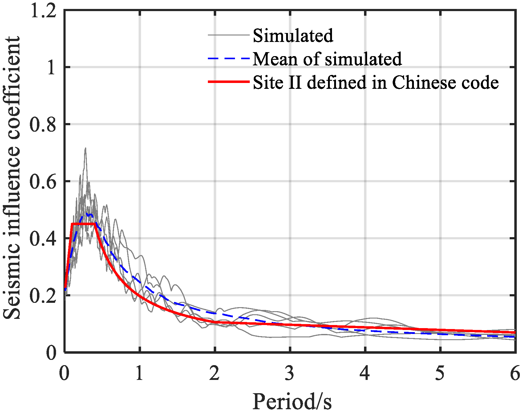
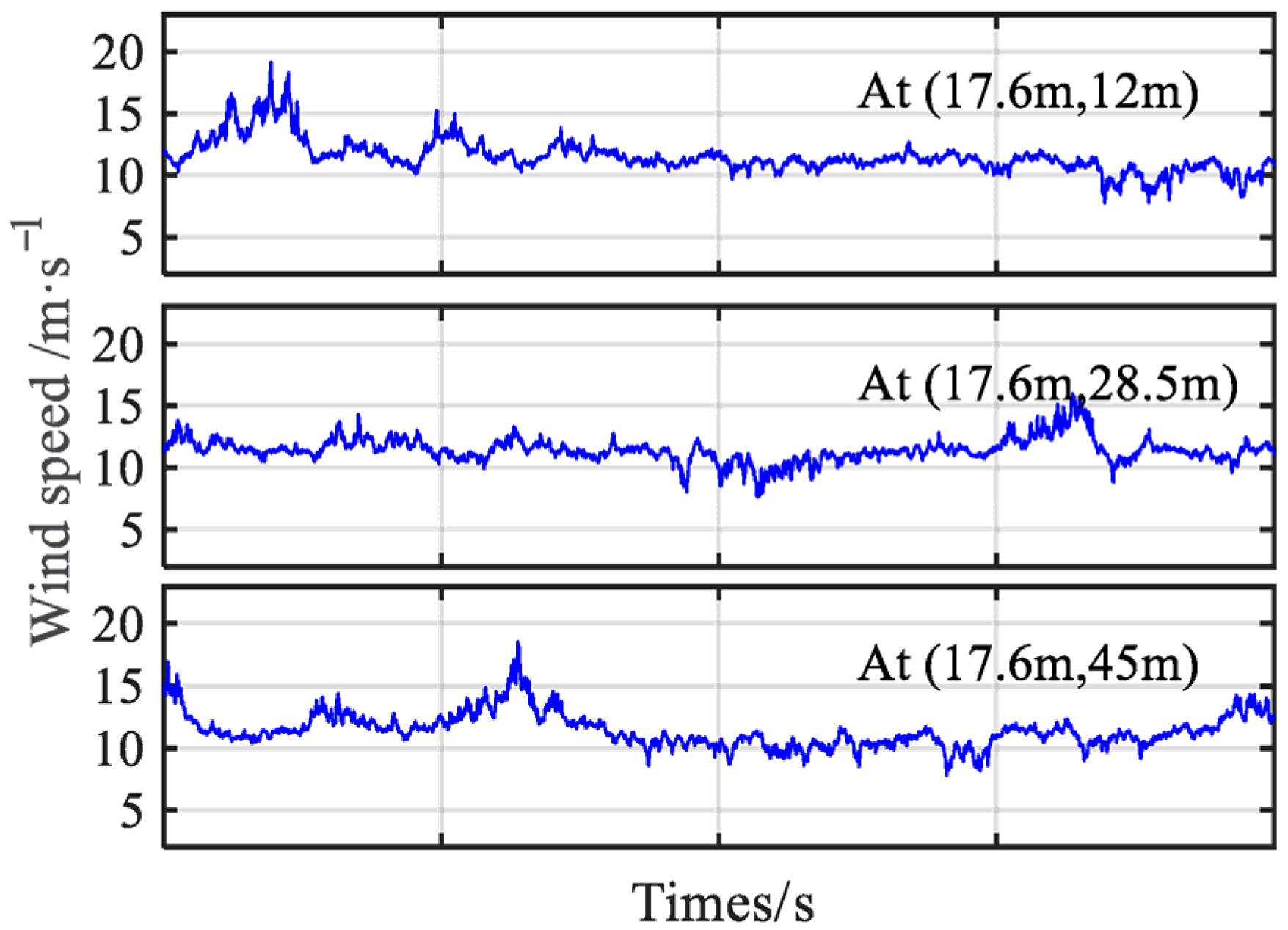
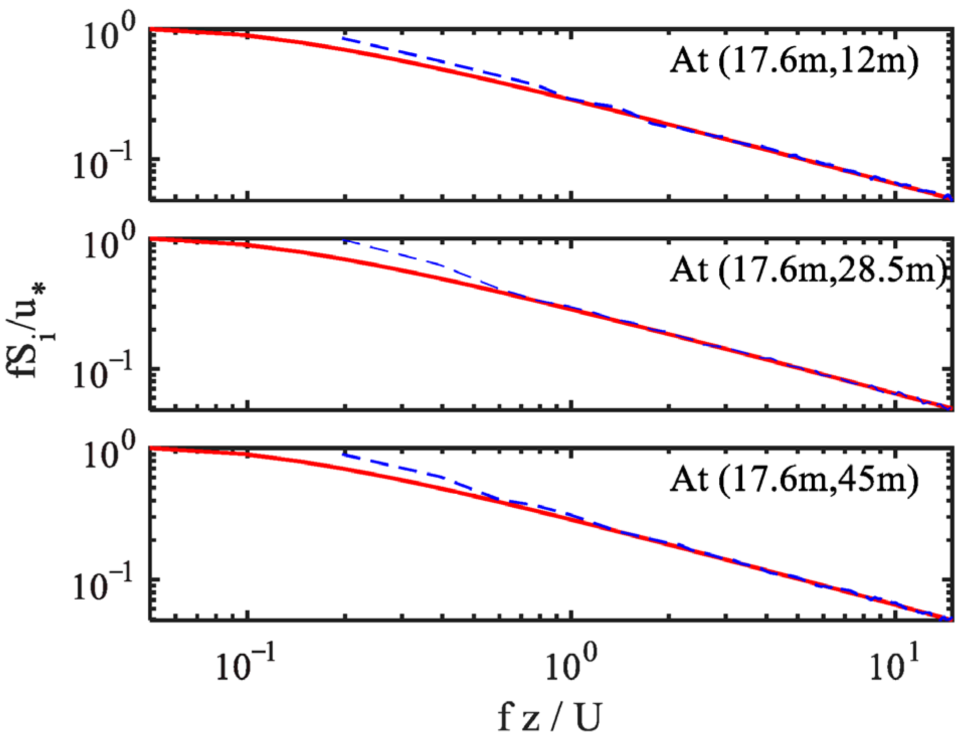
A typical time-history sample of offshore ground motion and response spectrum is shown in Figure 7 and Figure 8. It can be seen that the average response spectrum of simulated samples is close to that defined in the “Code for Seismic Design of Buildings” (GB 50011-2010), which demonstrates the applicability of simulation results. In addition, the non-Gaussian wind speed time histories at different heights are shown in Figure 9, and the comparison between the simulated PSD and the target values is shown in Figure 10. It can be seen that the two are extremely close, which proves the correctness of the simulation results.

5. Economic Loss Assessment and Risk Analysis of Coastal Building

5.1. Engineering Background

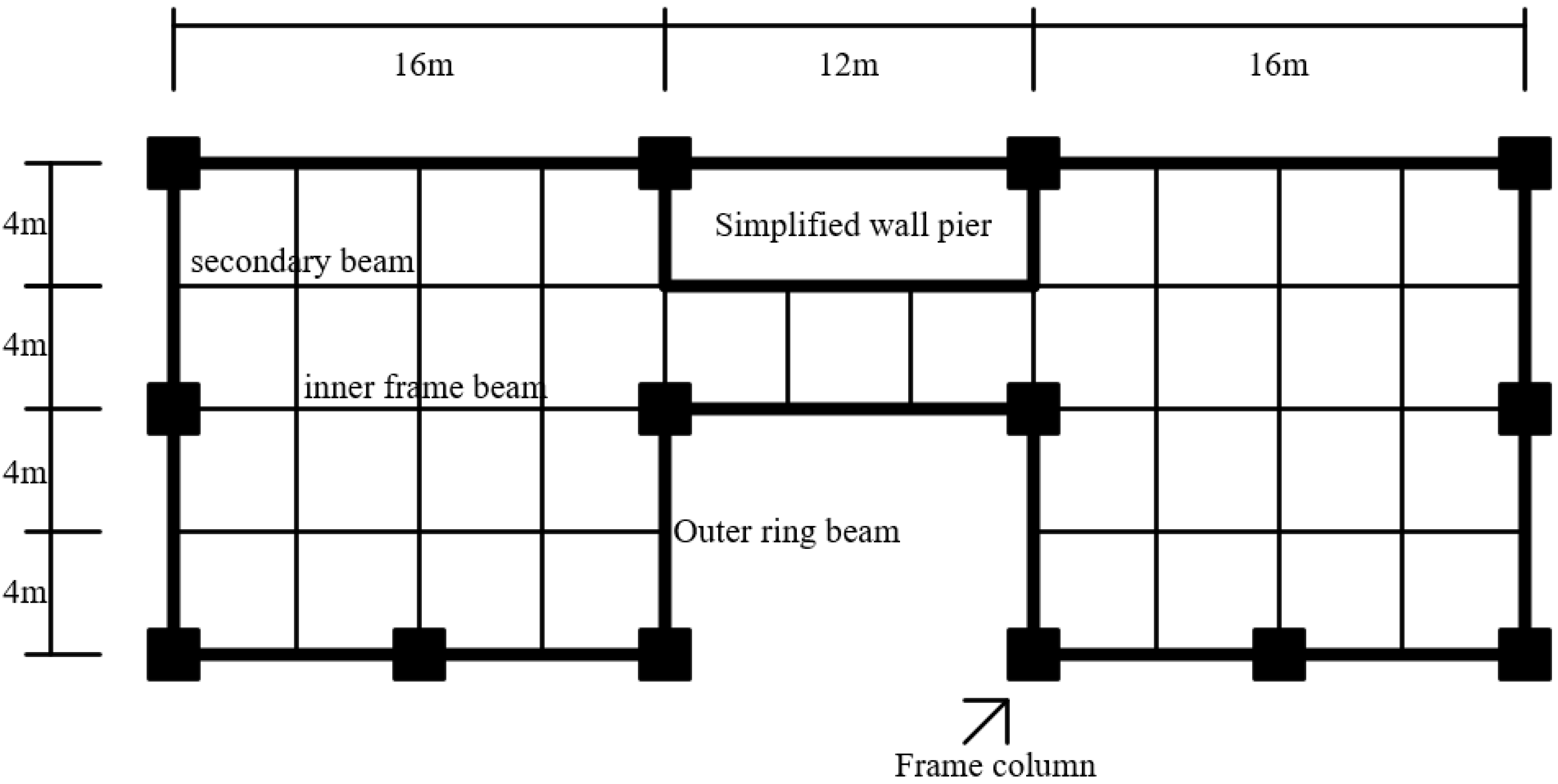
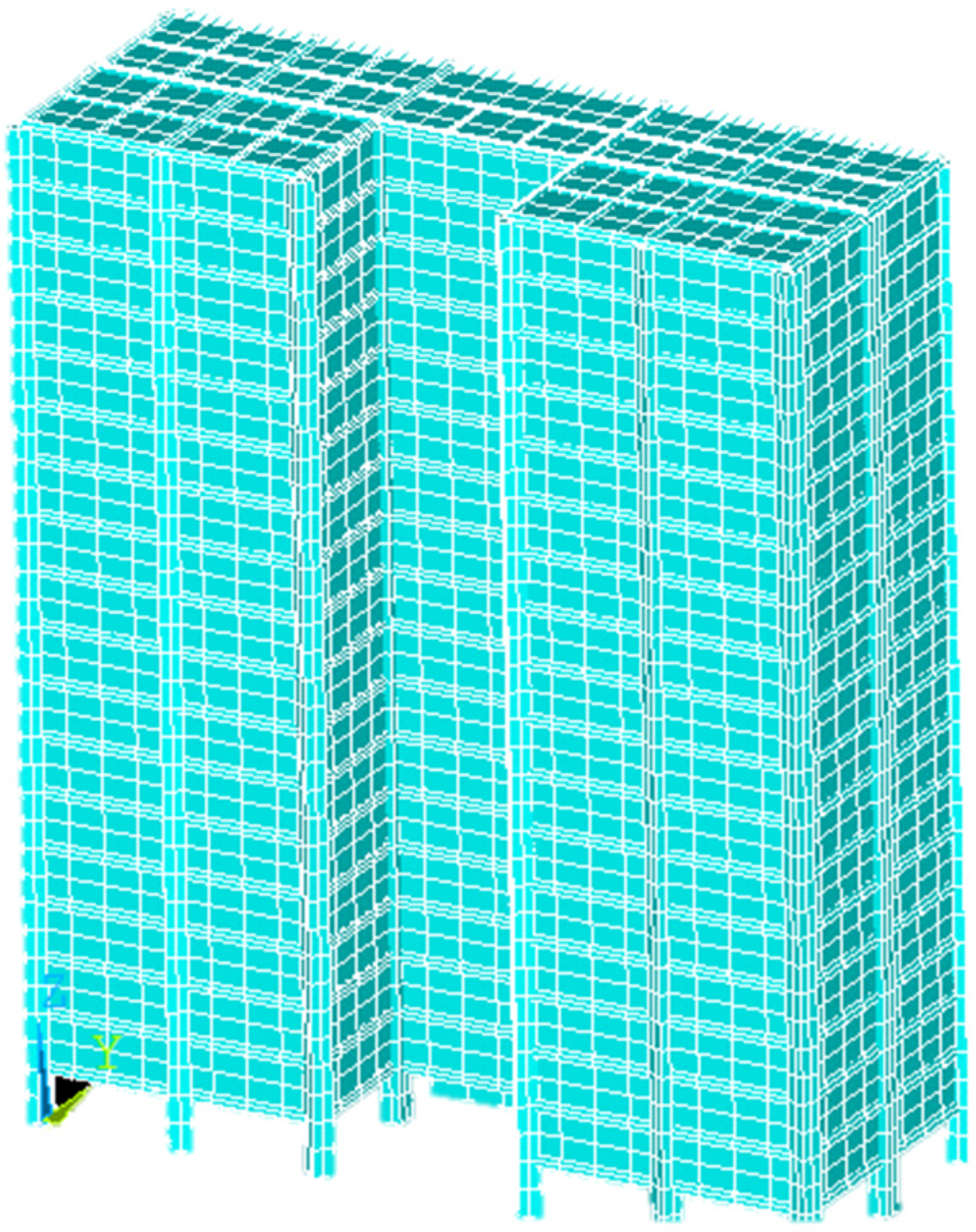
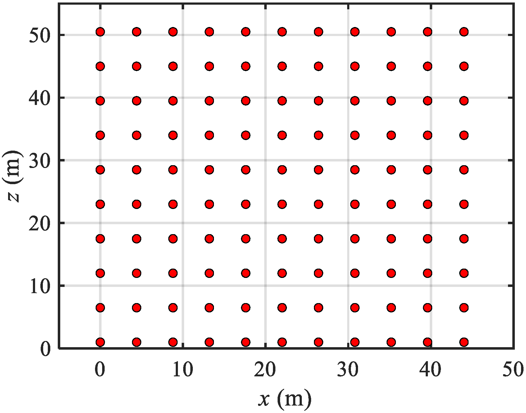
To assess the seismic economic loss of a nonlinear frame structure under the combined effects of offshore ground motion and non-Gaussian wind conditions, this study focuses on an 18-story high-rise frame structure with a floor height of 3 m. The structural layout is shown in Figure 11, with member sizes detailed in

Table 8. The section size of structural members.

Structural Members	Sections Size (m)	Concrete	Elastic Modulus (Pa)
Frame column	$1.1\times 1.1$	C40	$3.5\times {10}^{10}$
Outer ring beam	$0.4\times 0.6$	C40	$3.5\times {10}^{10}$
Inner frame beam	$0.5\times 0.8$	C40	$3.5\times {10}^{10}$
Secondary beam	$0.3\times 0.5$	C40	$3.5\times {10}^{10}$
Simplified wall pier	0.3	C40	$3.5\times {10}^{10}$
Roof panel	0.2	C30	$3.2\times {10}^{10}$
Peripheral wall	0.2	C30	$3.2\times {10}^{10}$

. For simplicity in calculations, the density of C30 and C40 reinforced concrete is assumed to be 2500 kg/m³, the elastic modulus is considered to be that of concrete, and the Poisson’s ratio is taken as 0.2. A finite element model, created using ANSYS17 software (Figure 12), employs BEAM188 elements for the columns and beams, and SHELL63 elements for the floors and exterior walls. The first six vibration modes are listed in

Table 9. The result of vibration mode analysis.

Order	1	2	3	4	5	6
Natural frequency (Hz)	1.70	2.75	3.36	5.83	7.01	7.15

, revealing that the first mode has a frequency of 1.70 Hz, indicating that the structure is flexible and susceptible to resonance with low-frequency loads, such as long-period ground motions. It is important to note that the elastic modulus is taken as the value for concrete for simplicity in calculations, which may result in a lower natural period for the structure. Additionally, the wind load application points on the frame structure are shown in Figure 13, with each loading point covering an area of approximately 20 m².

All column bases are fully fixed in translation and rotation to represent a deep, rigid foundation, and floor and roof slabs are modeled as rigid diaphragms to enforce in-plane stiffness and distribute lateral loads uniformly at each story. Rayleigh proportional damping is applied so that the first two vibration modes each exhibit a 5% modal damping ratio; the corresponding α and β coefficients are calculated from those undamped natural frequencies. Finally, three dynamic load cases—seismic-only, wind-only, and concurrent non-Gaussian wind plus seismic time-history analyses—are defined to assess the effects of varying hazard intensities on the frame structure.

5.2. Vulnerability-Based Failure Assessment Strategy

Incremental Dynamic Analysis (IDA) is a method used in dynamic time-history analysis to evaluate changes in a structure’s response under varying external excitation intensities. It establishes a quantitative relationship between the structure’s performance and the intensity of external excitations, revealing how these changes affect the overall structural performance. The general procedure for IDA is as follows [56,57,58]:

(1)

Determine the intensity index (IM) of external excitation, along with the PGA and average wind speed values considered in this study.

(2)

Determine the structural damage index (DM), focusing on the maximum story drift of the frame structure ${\theta }_{\max }$, which provides a clearer representation of the structural damage and performance states of its components.

(3)

Adjust the intensity of external excitation in equal steps, for example, using a range of 0.2 g to 1.0 g for the PGA, and varying wind speeds between 0 m/s and 20 m/s.

(4)

Simulate external excitation with varying intensities on the structure to determine the corresponding maximum story drift.

Actually, it can be acknowledged through the IDA method that there is an exponential correlation between the median value of the structural damage index with the intensity of external excitation index IM, and it can be described as follows:

$$\ln (\widehat{D})=A+B_1\ln (I{M}_1)+B_2\ln (I{M}_2)+\dots +B_N\ln (I{M}_N)$$

(28)

where $\widehat{D}$ indicates the median value of the structural damage index DM. A and $B_n$ are constants, and $I{M}_n$, $n=1,2,\dots ,N$ indicates the intensity index of the n-th external excitation.

Further, assumed that the disaster resilience of a structure at a certain level of performance is defined as C, and the structural response capacity of a structure under a certain intensity of external excitation is D. In that way, the structural failure probability can be written as follows [58]:

$$P_{\mathrm{f}}=P(R\le 0)=P(C/D\le 1)$$

(29)

Suppose that C and D correspond to a normal distribution, that is:

$$C~N({\mu }_C,{\sigma }_C)$$

(30)

$$D~N({\mu }_D,{\sigma }_D)$$

(31)

where ${\mu }_C$ and ${\sigma }_C$, respectively, denote the mean and standard deviation of disaster resilience, and ${\mu }_D$ and ${\sigma }_D$, respectively, denote the mean and standard deviation of structural response capacity. In the end, R also corresponds to the normal distribution, and its mean and standard deviation are $\mu ={\mu }_C-{\mu }_D$ and $\sigma =\sqrt{{\sigma }_C^2+{\sigma }_D^2}$. Further, convert R to the standard normal distribution; that is:

$$P_{\mathrm{f}}=P(R\le 0)=P(T\le {\displaystyle \frac{\mu }{\sigma }})=\mathsf{\Phi }({\displaystyle \frac{-\ln ({\mu }_C/{\mu }_D)}{\sqrt{{\beta }_C^2+{\beta }_D^2}}})$$

(32)

where ${\beta }_C$ and ${\beta }_D$, respectively, denote the logarithmic standard deviation. Actually, ${\mu }_D$ can be replaced by $\widehat{D}$ and ${\beta }_C^2=0.09$ as the intensity index IM of input external excitation, which is the significant wave height. Combining Equations (27) and (31), the calculation formula for failure probability can be written as follows [58]:

$$Z=P_{\mathrm{f}}=\mathsf{\Phi }[{\displaystyle \frac{\ln (\widehat{D})-\ln ({\mu }_c)}{\sqrt{{\beta }_D^2+0.09}}}]$$

(33)

$${\beta }_D=\sqrt{{\displaystyle \frac{{\displaystyle \sum _{n_{sel}}^{N_{sel}}{[\ln (D{M}_{n_{sel}})-\ln (\widehat{D})]}^2}}{N_{sel}-2}}}$$

(34)

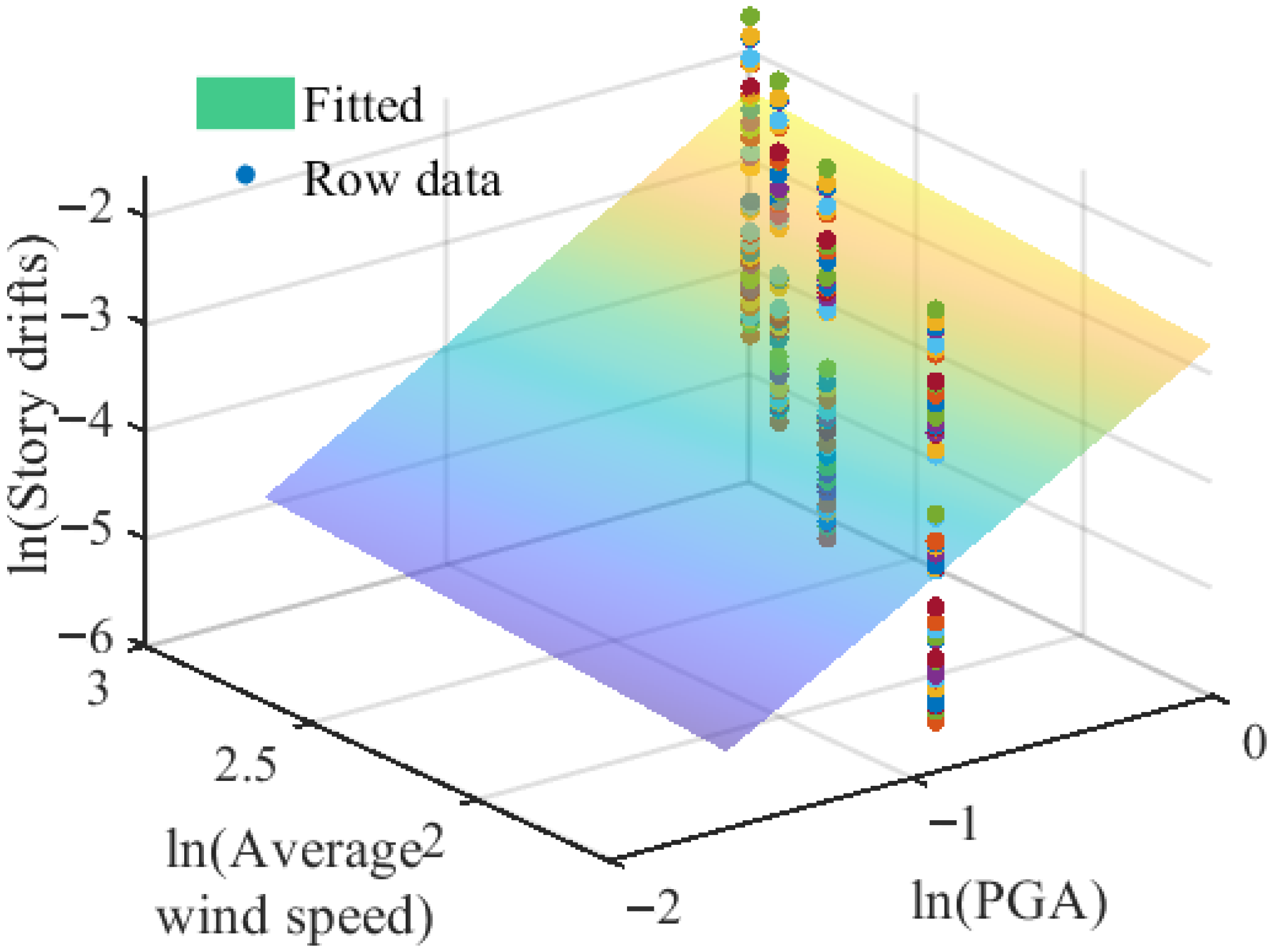
where $n_{sel}(1,2,\dots ,N_{sel})$ indicates the number of samples, and is taken as 20 in this numerical example. And the result of Equation (27) is shown in Figure 14, namely the fitted result of logarithmic average wind speed and PGA with the logarithmic story drifts, which demonstrates that there is a strong linear relationship between them, and the determination coefficient is 0.93, and A = −3.192, B₁ = 1.589, and B₂ = 0.2827.

Additionally, to evaluate the ultimate failure state of the structure, it is necessary to define the quantitative indicators for different failure states of the structural response. According to the “Code for Seismic Design of Buildings” (GB 50011-2010), the failure states of the frame structure are categorized into the following levels: intact, slightly damaged, moderately damaged, severely damaged, and collapsed. The corresponding descriptions for each level are as follows in

Table 10. The descriptions and quantitative indicators of each degree of structural damage.

Degree of Structural Damage		Descriptions	Quantitative Indicators (Inter-Story Drifts)
DS1	Slightly damaged	Hairline concrete cracks; No spalling or reinforcement damage; Minimal or no repairs required.	1/500
DS2	Moderately damaged	Visible cracks in beams and columns; Plaster or paint spalling; Minor non-structural damage (e.g., partition wall cracks); Repairs needed.	1/200
DS3	Severely damaged	Concrete cover spalling; Local reinforcement yielding; Moderate structural damage (e.g., stiffness loss, local loss of capacity); Repairable locally.	1/100
DS4	Collapsed	Plastic hinges formed; Extensive concrete spalling and element fracture; Severe structural failure or partial/total collapse.	1/50

.

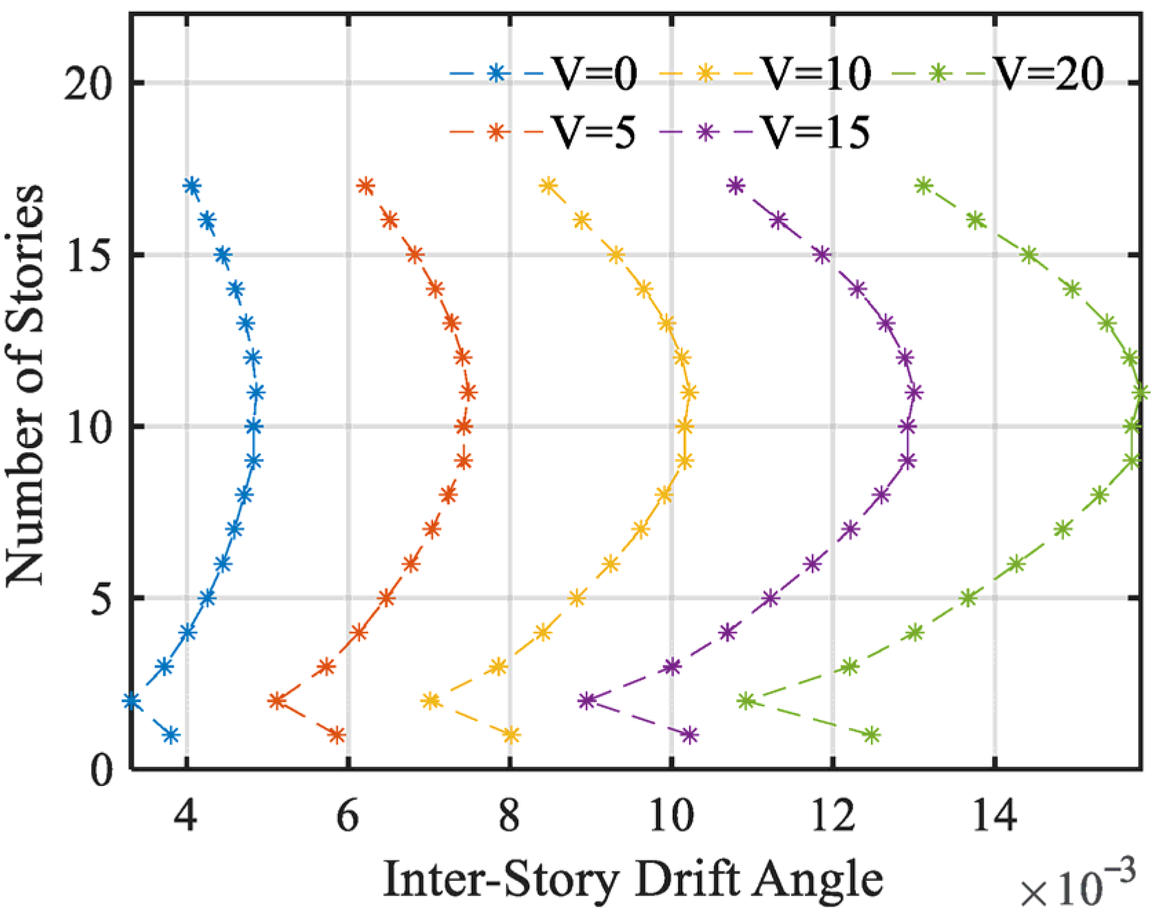
Figure 15 presents the inter-story drift angles for a structural frame under the combined effects of wind and seismic forces, with the analysis conducted for different wind speeds (V = 0, 5, 10, 15, and 20 m/s) at a constant PGA of 0.4 g. The data illustrates how the inter-story drift angle changes as wind speed increases, highlighting the structural vulnerability under various loading conditions. Under the condition of PGA = 0.4 g, the figure shows that when only considering the seismic load, the building reaches a moderate damage state (e.g., DS2), indicating that the structural damage is relatively mild under seismic forces alone. However, as the wind speed increases, especially when the wind speed reaches V = 15 and V = 20, the inter-story drift angle increases significantly, causing the structure to progress into higher damage states (such as DS3 and DS4). This suggests that when wind and seismic forces act simultaneously, the vulnerability of the structure is greatly amplified, and the presence of wind load exacerbates the effect of seismic forces, causing the structure to reach higher damage levels even under relatively low seismic loads. Therefore, considering only seismic loads may underestimate the actual vulnerability of the structure, and in multi-hazard scenarios, the combined effects of wind and earthquake forces must be fully accounted for to ensure structural safety.

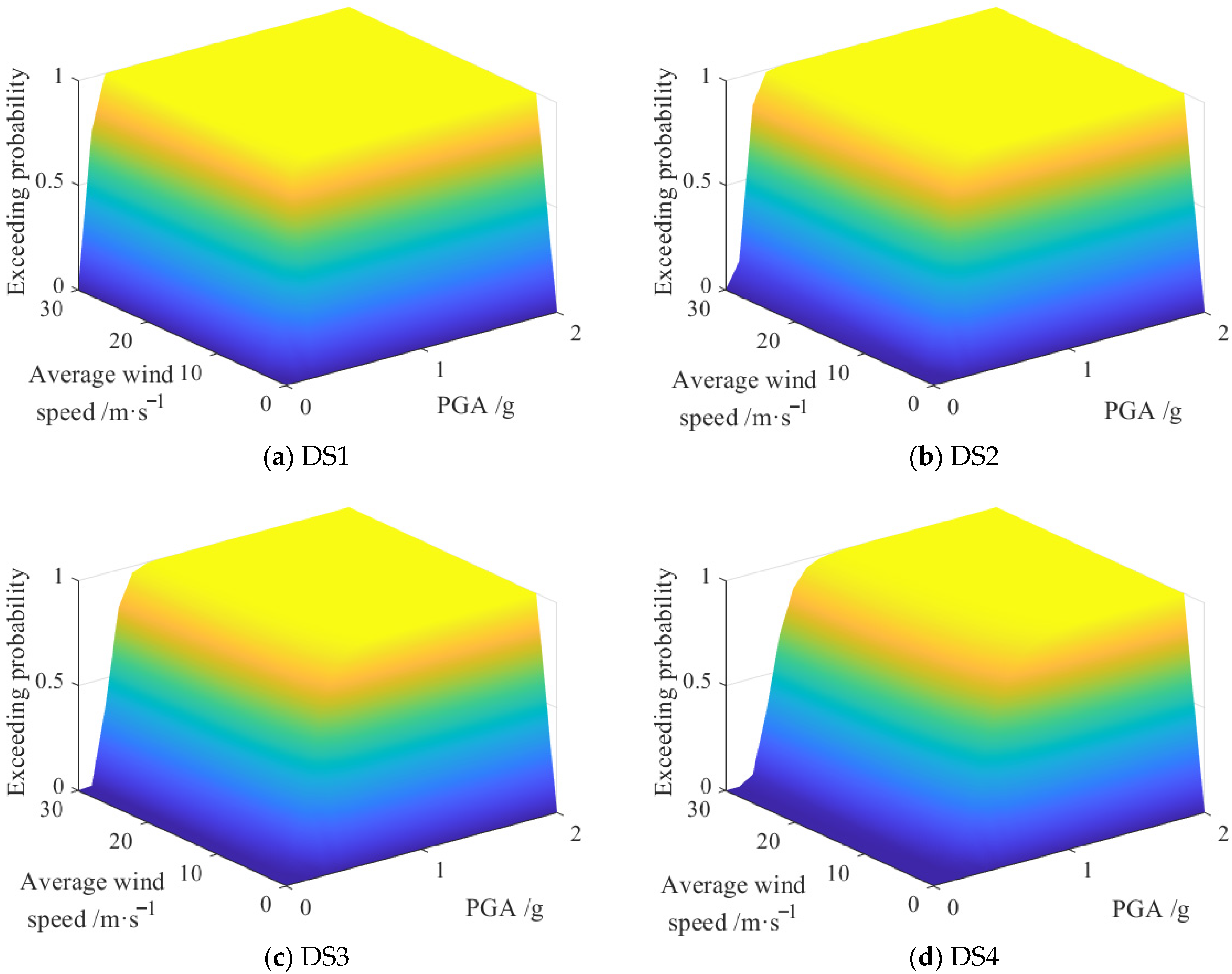
Figure 16 depicts the vulnerability surfaces of the structural frame under combined wind and seismic loading, across four damage limit states (DS1–DS4). Each surface shows the probability of exceeding a given damage threshold as a function of average wind speed (m/s) and peak ground acceleration (PGA, g). Several key insights emerge: Overall Trend: In all four limit states, the probability of damage occurrence rises with increasing wind speed and PGA, underscoring that intensified wind and seismic forces jointly elevate the risk of structural failure.

• DS1 (Light Damage): Here, the surface is most sensitive to PGA, especially at lower wind speeds, indicating that under relatively mild conditions, seismic action alone can provoke the first signs of damage, while wind remains a secondary influence.
• DS2 (Moderate Damage): The overall probability of exceeding the threshold is higher than in DS1, reflecting growing vulnerability. Wind speed begins to contribute more noticeably, though PGA continues to dominate the structural response.
• DS3 (Severe Damage): A sharp rise in damage probability is observed, particularly in regions of high PGA. Wind’s influence also becomes pronounced, signaling that as damage accumulates, the interaction between wind and seismic loads intensifies the extent of damage.
• DS4 (Collapse Threshold): The surface reaches its apex, with both high wind speeds and high PGA acting synergistically to drive failure. This state highlights the most critical vulnerabilities, where combined loading almost certainly leads to collapse.

In sum, these surfaces not only confirm that damage has already occurred at each limit state but also reveal a clear progression in the relative roles of seismic and wind forces. Lower damage states are primarily triggered by seismic events, whereas higher damage states demand an integrated, multi-hazard assessment to capture the complex interplay that ultimately compromises structural integrity.

5.3. Risk Analysis and Expected Economic Loss Assessment

Based on the fragility surface developed in Section 5.2, we proceed to quantify the structural risk by integrating it with the joint hazard model of seismic and wind intensities. This integration enables the estimation of the annual probability of exceeding various damage states under different return periods, thereby completing the full probabilistic risk assessment. The results are presented and discussed in the following Section.

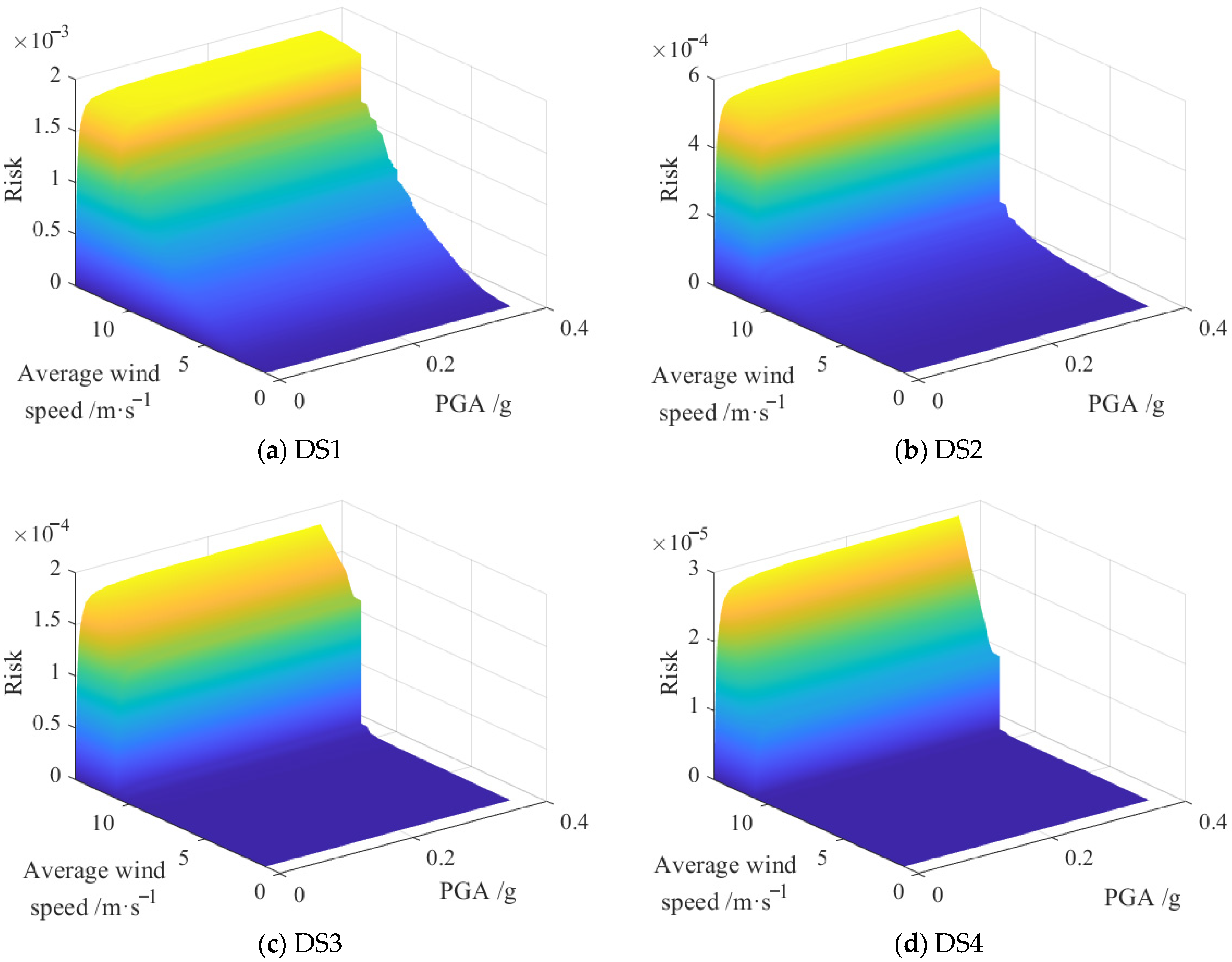
The risk integration method is different from only considering the hazard analysis of the disaster itself. This method calculates the convolution integral of the structural vulnerability and hazard curves to obtain risk-oriented disaster parameters. For multiple disasters, the risk score can be expressed as follows [59]:

$$v_i={\displaystyle {\int }_0^{30}{\displaystyle {\int }_0^{2}P(x,y)z_i(x,y)\mathrm{d}x\mathrm{d}y}}$$

(35)

where $v_i$ indicates the risk. $P(x,y)$ indicates the Hazard model, and the co-occurrence model defined in Equation (14) is considered. $z_i(x,y)$ indicates the probability distribution function of the structural vulnerability function under multiple disasters of the i-th failure state.

According to the aforementioned hazard analysis and vulnerability analysis, the risk of each failure state is shown in Figure 17. The risk surfaces in this figure illustrate the impact of both wind speed and peak ground acceleration (PGA) on the structural integrity under four distinct damage states (DS1 to DS4). Wind plays a significant role in shaping the risk profile across all these states, with its influence being particularly pronounced in the earlier damage states. In DS1, where the structure is most vulnerable, wind speed has a dominant impact on risk. The risk surface rises sharply with increasing wind speed, especially when combined with moderate PGA values. Even at low seismic intensities, a high wind speed dramatically amplifies the structural risk, suggesting that wind loads pose a critical threat to structural safety in this damage state. This highlights that, under DS1 conditions, the structure’s sensitivity to wind-induced forces is higher than that to seismic forces, especially when PGA remains low. As the damage progresses to DS2, wind speed continues to exert a significant influence on the risk levels. Although the PGA also starts to play a more prominent role, the wind’s impact remains critical, particularly at higher wind speeds. The overall risk is still high, approaching values similar to those in DS1, but the risk surface becomes slightly smoother, indicating a more gradual rise in risk compared to DS1. This suggests that while wind remains a key factor, the structure’s resilience to wind loads improves slightly as it transitions from DS1 to DS2. In DS3, the effect of wind speed begins to diminish compared to the earlier damage states, but it is still notable. The risk surface is less steep, meaning that while wind speed increases the risk, the rate at which the risk rises is slower than in DS1 and DS2. PGA becomes more influential in driving the risk in this state, but the wind’s contribution is still evident, particularly in cases of high wind speeds combined with moderate seismic activity. The structural risk remains sensitive to wind-induced loads, though the effect is tempered. Finally, in DS4, the overall risk is minimal, and wind speed has a relatively reduced impact compared to earlier states. The risk surface is flatter, indicating that the structure is more robust against both wind and seismic loads in this state. However, even in this least vulnerable state, wind speed still slightly influences the risk, particularly when seismic activity is low. The risk associated with high wind speeds is far lower than in the previous states, underscoring the structure’s improved capacity to withstand external forces in this stage. In summary, wind speed is a major determinant of structural risk, particularly in the early damage states where the structure is highly sensitive to wind-induced loads. As the damage state progresses, the influence of wind speed decreases, but it remains a key factor in determining the overall risk, particularly when coupled with seismic activity. The analysis of these risk surfaces highlights the critical role that wind forces play in structural safety under varying damage conditions, with the most pronounced effects observed in the more vulnerable damage states.

As the risk of each failure state is obtained, the expected economic loss can be calculated by the following method:

$$EL=b_1(Z_2-Z_1)+b_2(Z_3-Z_2)+b_3(Z_4-Z_3)+b_4{Z}_4$$

(36)

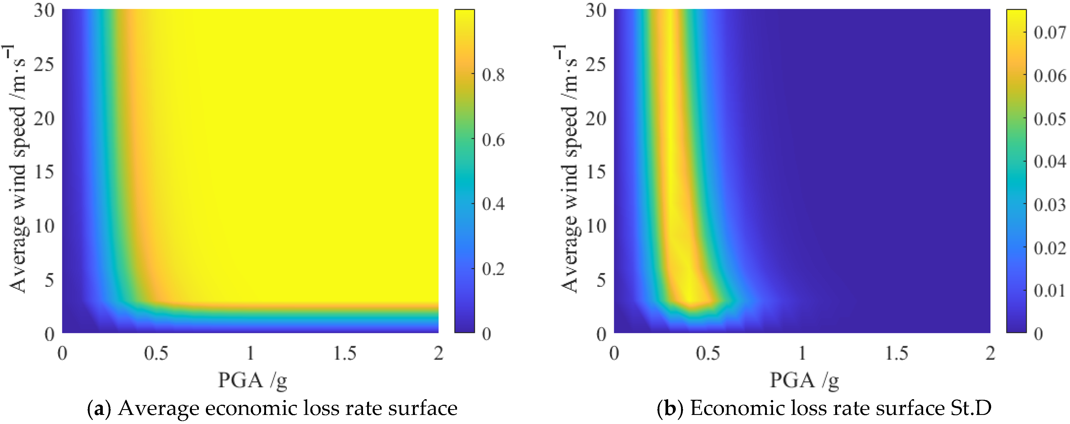
where $b_i$ indicates the expected economic loss coefficient of each failure state, and is, respectively, taken as 0.11, 0.31, 0.73, and 1 for DS1~DS4 [60]. Further, to investigate the impact of loss ratio variability on the economic loss assessment, a Monte Carlo simulation was performed under the assumption that the loss ratios for each damage state follow a normal distribution. The mean values of the loss ratios for DS1 to DS3 were set as 0.11, 0.31, and 0.73, respectively. A coefficient of variation (COV) of 0.2 was adopted for each stage to reflect moderate uncertainty in practical engineering applications. For each simulation, a random set of loss ratios was sampled according to the corresponding distributions, and the expected economic loss ratio was calculated. This process was repeated 10,000 times to obtain the distribution and variability range of the economic loss ratio. The results provide a quantitative measure of how loss ratio uncertainty propagates to the economic loss analysis, offering insight into the robustness and reliability of the risk evaluation.

Figure 18a presents the mean economic loss ratio of the structure across the space defined by average wind speed and PGA. The results show that the mean loss ratio increases rapidly with rising PGA, especially within the low to moderate PGA range, and then quickly saturates at higher values. This indicates that seismic intensity is the dominant factor controlling the expected economic loss, while the effect of wind speed becomes less significant once the PGA exceeds a certain threshold. In regions of low PGA and low wind speed, the mean loss ratio remains low, reflecting minor structural damage and negligible loss. Figure 18b depicts the standard deviation of the economic loss ratio, thereby illustrating the uncertainty introduced by the variability of loss ratios for different damage states. The standard deviation is highest in the transition zone, where the mean loss ratio experiences a sharp increase, particularly at low to moderate PGA values and lower wind speeds. This suggests that uncertainty in economic loss assessment is most significant in scenarios with intermediate hazard levels, where both damage probability and loss variability interact. In contrast, in areas with either very high or very low PGA and wind speed, the standard deviation diminishes, implying that economic loss predictions become more robust and less sensitive to loss ratio uncertainty in these regions.

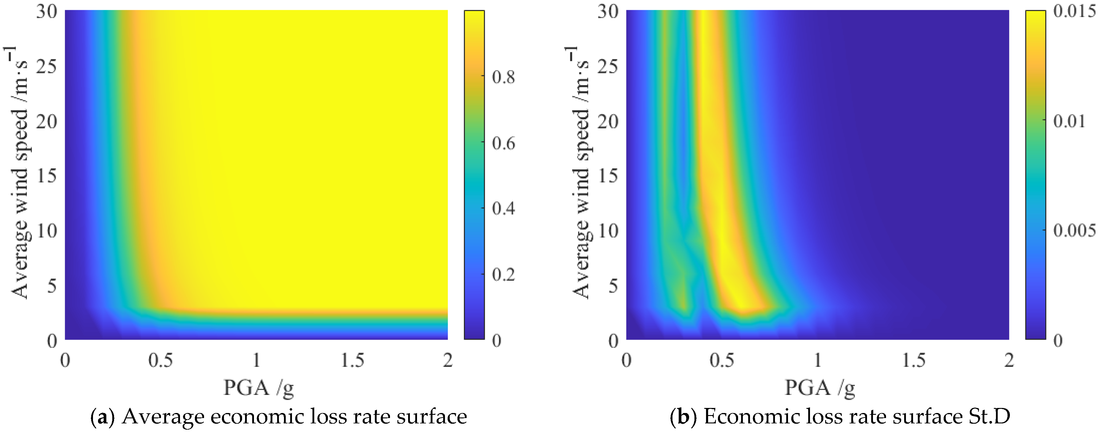
By further incorporating the randomness of the economic loss coefficient—specifically, treating the elastic modulus of concrete as a lognormally distributed variable with a coefficient of variation of 0.2, the mean value of the elastic parameter is taken from Table 7—this study evaluates the combined effect of material property uncertainty and loss ratio variability on the economic loss assessment. The advanced point selection method based on number theory was adopted to efficiently sample the probability space, improving simulation convergence and representativeness compared to traditional Monte Carlo approaches [60]. Figure 19a presents the mean economic loss ratio under the joint influence of both uncertainties. The results reveal that, consistent with previous findings, the mean loss ratio increases rapidly with PGA and quickly approaches saturation as the seismic intensity rises. The effect of wind speed remains limited, particularly at higher PGA values where the loss ratio plateaus. Figure 19b displays the standard deviation of the economic loss ratio, reflecting the overall uncertainty in the assessment. Compared to scenarios considering only loss ratio randomness, the standard deviation is slightly elevated, especially in the transition zones (low to moderate PGA and wind speed). This highlights that the inclusion of structural parameter variability further amplifies the uncertainty in economic loss predictions, particularly in regions where the transition from minor to severe damage occurs. Nevertheless, in domains where the economic loss ratio is either very low or nearly saturated, the overall uncertainty remains small. These results underscore the importance of accounting for both structural and economic uncertainties to achieve a robust and comprehensive risk evaluation for engineering structures under coupled wind and seismic hazards.

Based on the saturation behavior observed, a design PGA threshold of 0.5 g is recommended for cost optimization. Beyond this level, the additional investment required to increase seismic capacity yields negligible decreases in expected loss. This approach can be readily extended to critical underground structures: the loss-ratio saturation PGA should be identified via dynamic loss simulations, and the seismic design spectrum set accordingly to balance retrofit costs and risk reduction

5.4. Practical Implications

To demonstrate how this integrated wind–seismic risk framework can be applied in real-world engineering practice, we highlight below five key practical implications for design, regulation, emergency response, finance, and asset management:

• Performance-based Structural Design: Practicing engineers can import the unified hazard curves and damage-state probabilities into design tools to size members, detail connections, and select dampers that meet combined wind–seismic performance targets rather than conservative single-hazard checks.
• Code and Guideline Development: Standards committees can adopt the four consistency-based return-period metrics (single, co-occurrence, encounter, combination) to set unified multi-hazard design criteria, replacing separate wind and seismic provisions.
• Emergency Planning and Resilience: Disaster planners can define multi-hazard alert levels and evacuation thresholds based on co-occurrence and encounter functions, and allocate response resources using the damage-state probability distributions.
• Risk Management and Insurance: Insurers and asset owners can calibrate premiums and resilience investments by quantifying expected annualized losses under realistic compound-event scenarios.
• Asset Maintenance and Retrofit Prioritization: Facility managers can use the vulnerability and risk surfaces to rank buildings by combined hazard risk, targeting retrofit budgets where the marginal reduction in expected loss is greatest.

6. Conclusions

This study investigates the joint recurrence period of earthquake and wind hazards at a coastal site, assessing the vulnerability and economic impacts on a high-rise frame structure. The findings demonstrate that the integrated application of maximum entropy theory and Copula functions provides an effective approach for evaluating the hazard intensity and recurrence intervals of submarine earthquakes and strong wind events. For the PGA marginal distribution, our sixth-moment maximum-entropy model achieved an R² of 0.90, compared with 0.57 for a conventional GEV fit—reflecting a 58% increase in explained variance. Among the various models considered, the co-occurrence model exhibits superior performance over encounter, combined, and single-hazard models. The analysis indicates that, under a 0.4 g ground motion and a simultaneous wind speed of 15 m/s, the probabilities of slight, moderate, severe, and collapse damage are approximately 2 × 10⁻³, 6 × 10⁻⁴, 2 × 10⁻⁴, and 3 × 10⁻⁵, respectively. Furthermore, both the randomness of structural parameters and the uncertainty of economic loss ratios are found to significantly influence the economic loss ratio, with the greatest variability—reaching up to 0.015—observed within the 0.2 g to 0.4 g seismic intensity range, where seismic action predominates.

The strengths of this article lie in its innovative integration of advanced probabilistic models and real-world hazard data to assess the compound risks facing coastal structures, as well as its clear quantification of both hazard and economic impacts. The use of joint probabilistic modeling and the consideration of multiple sources of uncertainty represent significant advances in multi-hazard risk assessment. However, the study could be further strengthened by incorporating more detailed modeling of earthquake frequency spectra, the nonlinear response of high-rise structures, and a broader analysis of material variability. Addressing these areas in future work will enhance the accuracy and applicability of the proposed framework for practical engineering design and disaster mitigation.

This study assumes a single wind direction and rigid foundation, neglecting wind-direction variability, multi-directional loading effects, and soil–structure interaction (SSI). It also lacks direct validation against field or experimental data and models only a regular frame without plan irregularities or core-wall systems. Future work will introduce multi-directional wind fields and SSI, calibrate the framework using measured and experimental results, and extend its application to tunnels, bridges, and other complex structural configurations. Despite these limitations, the proposed joint risk assessment workflow provides valuable guidance for design practice, code development, and emergency planning.

References

1. Ru, J.; Liu, J.; Qu, J.; Li, J. Architecture Environmental and Civil Engineering; China Architecture & Building Press: Beijing, China, 2011. [Google Scholar]
2. Akiyama, M. Life-cycle approaches to sustainable and resilient infrastructure: Innovations in multi-hazard frameworks. Struct. Infrastruct. Eng. 2025, 1–26. [Google Scholar] [CrossRef]
3. Wang, J.; He, Z.; Weng, W. A review of the research into the relations between hazards in multi-hazard risk analysis. Nat. Hazards 2020, 104, 2003–2026. [Google Scholar] [CrossRef]
4. Verschuur, J.; Koks, E.E.; Li, S.; Hall, J.W. Multi-hazard risk to global port infrastructure and resulting trade and logistics losses. Commun. Earth Environ. 2023, 4, 5. [Google Scholar] [CrossRef]
5. Wu, G.Y.; Liu, C.G.; Dong, Z.Q.; Liu, H.-D.; Ali, F. Multihazard resilience and economic loss evaluation method for cable-stayed bridges under the combined effects of scour and earthquakes. Eng. Struct. 2024, 314, 118033. [Google Scholar] [CrossRef]
6. Nofal, O.M.; Amini, K.; Padgett, J.E.; van de Lindt, J.W.; Rosenheim, N.; Darestani, Y.M.; Enderami, A.; Sutley, E.J.; Hamideh, S.; Duenas-Osorio, L. Multi-hazard socio-physical resilience assessment of hurricane-induced hazards on coastal communities. Resilient Cities Struct. 2023, 2, 67–81. [Google Scholar] [CrossRef]
7. Laino, E.; Iglesias, G. Multi-hazard assessment of climate-related hazards for European coastal cities. J. Environ. Manag. 2024, 357, 120787. [Google Scholar] [CrossRef]
8. Argyroudis, S.A.; Mitoulis, S.A.; Hofer, L.; Zanini, M.A.; Tubaldi, E.; Frangopol, D.M. Resilience assessment framework for critical infrastructure in a multi-hazard environment: Case study on transport assets. Sci. Total Environ. 2020, 714, 136854. [Google Scholar] [CrossRef] [PubMed]
9. Li, H.; Zheng, X.; LI, C. Research progress on life-cycle multihazard-based design theory for high-performance structures. J. Build. Struct. 2019, 40, 56–69. (In Chinese) [Google Scholar] [CrossRef]
10. Yang, Q.; Li, H.; Zhang, L.; Guo, K.; Li, K. Nonlinear flutter in a wind-excited double-deck truss girder bridge: Experimental investigation and modeling approach. Nonlinear Dyn. 2025, 113, 6427–6445. [Google Scholar] [CrossRef]
11. Gong, B.; Li, H. A couple Voronoi-RBSM modeling strategy for RC structures. Struct. Eng. Mech. 2024, 91, 239–250. [Google Scholar] [CrossRef]
12. Li, J.; Hu, Z.; Cui, J.; Lin, G. Efficient GPU-accelerated seismic analysis strategy and scenario simulation for large-scale nuclear structure cluster-soil interaction over ten million DOFs. Comput. Geotech. 2024, 174, 106583. [Google Scholar] [CrossRef]
13. Zhang, Z.; Guo, F.; Gao, J.; Deng, E.; Kong, J.; Zhang, L. Seismic performance of an innovative prefabricated bridge pier using rapid hardening ultra-high performance concrete. Structures 2025, 74, 108558. [Google Scholar] [CrossRef]
14. Kazemi, F.; Asgarkhani, N.; Jankowski, R. Machine learning-based seismic fragility and seismic vulnerability assessment of reinforced concrete structures. Soil Dyn. Earthq. Eng. 2023, 166, 107761. [Google Scholar] [CrossRef]
15. Smith, V.; Mahmoud, H. Multihazard assessment of wind turbine towers under simultaneous application of wind, operation, and seismic loads. J. Perform. Constr. Facil. 2016, 30, 04016043. [Google Scholar] [CrossRef]
16. Mensah, A.F.; Duenas-Osorio, L.; Prowell, I.; A Asareh, M. Probabilistic Combination of Earthquake and Operational Loads for Wind Turbines. In Proceedings of the 15th World Conference on Earthquake Engineering, Lisbon, Portugal, 24–28 September 2012. [Google Scholar] [CrossRef]
17. Venanzi, I.; Lavan, O.; Ierimonti, L.; Fabrizi, S. Multi-hazard loss analysis of tall buildings under wind and seismic loads. Struct. Infrastruct. Eng. 2018, 14, 1295–1311. [Google Scholar] [CrossRef]
18. Venanzi, I.; Lavan, O.; Fabrizi, S. Multi-Hazard Life-Cycle Performance of Tall Buildings Under Seismic and Wind Loads. In Life-Cycle of Engineering Systems: Emphasis on Sustainable Civil Infrastructure; CRC Press: Boca Raton, FL, USA, 2016; 9781315375175. [Google Scholar]
19. Dogruel, S.; Dargush, G.F. A Framework for Multi-Hazard Design and Retrofit of Passively Damped Structures. In Proceedings of the Architectural Engineering Conference (AEI) 2008, Denver, CO, USA, 24–27 September 2008. [Google Scholar] [CrossRef]
20. Athanasiou, A.; Tirca, L.; Stathopoulos, T. Performance-based wind and earthquake design framework for tall steel buildings with ductile detailing. J. Wind. Eng. Ind. Aerodyn. 2023, 240, 105492. [Google Scholar] [CrossRef]
21. Ciabattoni, M.; Petrini, F.; Pampanin, S. Multi-hazard design of low-damage high-rise steel–timber buildings subjected to wind and earthquake loading. Eng. Struct. 2024, 303, 117522. [Google Scholar] [CrossRef]
22. Lin, J.W. An empirical correlation between the occurrence of earthquakes and typhoons in Taiwan: A statistical multivariate approach. Nat. Hazards 2013, 65, 605–634. [Google Scholar] [CrossRef]
23. Steer, P.; Jeandet, L.; Cubas, N.; Marc, O.; Meunier, P.; Simoes, M.; Cattin, R.; Shyu, J.B.H.; Mouyen, M.; Liang, W.-T.; et al. Earthquake statistics changed by typhoon-driven erosion. Sci. Rep. 2020, 10, 10899. [Google Scholar] [CrossRef]
24. Nanjo, K.Z. Were changes in stress state responsible for the 2019 Ridgecrest, California, earthquakes? Nat. Commun. 2020, 11, 3082. [Google Scholar] [CrossRef] [PubMed]
25. Ming, X.; Xu, W.; Li, Y.; Du, J.; Liu, B.; Shi, P. Quantitative multi-hazard risk assessment with vulnerability surface and hazard joint return period. Stoch. Environ. Res. Risk Assess. 2015, 29, 35–44. [Google Scholar] [CrossRef]
26. Wei, L.; Hu, K.; Hu, X.; Wu, C.; Zhang, X. Quantitative multi-hazard risk assessment to buildings in the Jiuzhaigou valley, a world natural heritage site in Western China. Geomat. Nat. Hazards Risk 2022, 13, 193–221. [Google Scholar] [CrossRef]
27. Hu, X.; Fang, G.; Ge, Y. Joint probability analysis and mapping of typhoon-induced wind, wave, and surge hazards along southeast China. Ocean. Eng. 2024, 311, 118844. [Google Scholar] [CrossRef]
28. Xu, Y.; Becker, T.C.; Guo, T. Design optimization of triple friction pendulums for high-rise buildings considering both seismic and wind loads. Soil Dyn. Earthq. Eng. 2021, 142, 106568. [Google Scholar] [CrossRef]
29. Tan, J.; Hu, J. Offshore ground motion characteristics on the horizontal PGA, spectral acceleration, frequency content and significant duration from the 2021 Mw 7.1 and 2022 Mw 7.4 offshore earthquakes near the Japan Trench area. Soil Dyn. Earthq. Eng. 2023, 164, 107646. [Google Scholar] [CrossRef]
30. Chen, B.; Wang, D.; Chen, S.; Hu, S. Influence of site factors on offshore ground motions: Observed results and numerical simulation. Soil Dyn. Earthq. Eng. 2021, 145, 106729. [Google Scholar] [CrossRef]
31. Ma, X.; Xu, F. An efficient simulation algorithm for non-Gaussian stochastic processes. J. Wind. Eng. Ind. Aerodyn. 2019, 194, 103984. [Google Scholar] [CrossRef]
32. Zhou, H.; Deodatis, G.; Shields, M.; Benowitz, B. Simulation of wind velocity time histories on long span structures modeled as non-Gaussian stochastic waves. Probabilistic Eng. Mech. 2020, 59, 103016. [Google Scholar] [CrossRef]
33. Shields, M.D.; Deodatis, G. A simple and efficient methodology to approximate a general non-Gaussian stationary stochastic vector process by a translation process with applications in wind velocity simulation. Probabilistic Eng. Mech. 2013, 31, 19–29. [Google Scholar] [CrossRef]
34. Ibsen, L.B.; Asgari, A.; Bagheri, M.; Barari, A. Response of monopiles in sand subjected to one-way and transient cyclic lateral loading. In Proceedings of the Geotechnical Special Publications, Atlanta, GA, USA, 23–26 February 2014; pp. 312–322. [Google Scholar] [CrossRef]
35. Asgari, A.; Bagheri, M.; Hadizadeh, M. Advanced seismic analysis of soil-foundation-structure interaction for shallow and pile foundations in saturated and dry deposits: Insights from 3D parallel finite element modeling. Structures 2024, 69, 107503. [Google Scholar] [CrossRef]
36. Arjomand, M.A.; Bagheri, M.; Mostafaei, Y. Performance Enhancement of Tuned Liquid Dampers in Fixed Offshore Platforms: A Coupled ANSYS Aqwa-Transient Structural Approach. Civ. Eng. Appl. Solut. 2025, 1, 78–88. [Google Scholar]
37. GB 50011-2010; Code for Seismic Design of Buildings. Architecture and Building Press: Beijing, China, 2016.
38. Shannon, C.E. A mathematical theory of communication. Bell Syst. Tech. J. 1948, 27, 379–423. [Google Scholar] [CrossRef]
39. Berrill, J.B.; Davis, R.O. Maximum Entropy and the Magnitude Distribution. Bull. Seismol. Soc. Am. 1980, 70, 1823–1831. [Google Scholar]
40. Kotz, S.; Nadarajah, S. Multivariate Extreme Value Distributions. In Extreme Value Distributions: Theory and Applications; Imperial College Press: London, UK, 2000; Volume 191, pp. 95–150. [Google Scholar] [CrossRef]
41. Sklar, M. Fonctions de répartition à n dimensions et leurs marges. Ann. L’isup 1959, 8, 229–231. Available online: https://hal.science/hal-04094463/document (accessed on 22 August 2025).
42. Huard, D.; Evin, G.; Favre, A.C. Bayesian copula selection. Comput. Stat. Data Anal. 2006, 51, 809–822. [Google Scholar] [CrossRef]
43. Fan, Y.R.; Yu, L.; Shi, X.; Duan, Q.Y. Tracing Uncertainty Contributors in the Multi-Hazard Risk Analysis for Compound Extremes. Earth’s Future 2021, 9, e2021EF002280. [Google Scholar] [CrossRef]
44. Zhang, Y.; Li, Y.; Dong, Y. Probabilistic analysis of long-term loss incorporating maximum entropy method and analytical higher-order moments. J. Infrastruct. Preserv. Resil. 2022, 3, 7. [Google Scholar] [CrossRef]
45. Kazemi, F.; Asgarkhani, N.; Jankowski, R. Machine learning-based seismic response and performance assessment of reinforced concrete buildings. Arch. Civ. Mech. Eng. 2023, 23, 94. [Google Scholar] [CrossRef]
46. Priestley, M.B. Evolutionary spectra and non-stationary processes. J. R. Stat. Soc. Ser. B 1965, 27, 204–237. [Google Scholar] [CrossRef]
47. Amin, M.; Ang, A.H.S. Nonstationary stochastic models of earthquake motions. J. Eng. Mech. Div. 1968, 94, 559–584. [Google Scholar] [CrossRef]
48. Clough, R.W.; Penzien, J. Dynamic of Structures; McGraw-Hill Inc.: New York, NY, USA, 1993. [Google Scholar]
49. Deodatis, G. Non-stationary stochastic vector processes: Seismic ground motion applications. Probabilistic Eng. Mech. 1996, 11, 149–167. [Google Scholar] [CrossRef]
50. Shinozuka, M.; Jan, C.M. Digital simulation of random processes and its applications. J. Sound Vib. 1972, 25, 111–128. [Google Scholar] [CrossRef]
51. Grigoriu, M. Crossings of non-Gaussian translation processes. J. Eng. Mech. 1984, 110, 610–620. [Google Scholar] [CrossRef]
52. Simiu, E.; Scanlan, R.H. Wind Effects on Structures: An Introduction to Wind Engineering; Wiley: New York, NY, USA, 1978. [Google Scholar]
53. Kaimal, J.C.; Wyngaard, J.C.; Izumi, Y.; Coté, O.R. Spectral characteristics of surface-layer turbulence. Q. J. R. Meteorol. Soc. 1972, 98, 563–589. [Google Scholar] [CrossRef]
54. Davenport, A.G. The spectrum of horizontal gustiness near the ground in high winds. Q. J. R. Meteorol. Soc. 1961, 87, 194–211. [Google Scholar] [CrossRef]
55. Shinozuka, M.; Deodatis, G. Simulation of multi-dimensional Gaussian stochastic fields by spectral representation. Appl. Mech. Rev. 1996, 49, 29–53. [Google Scholar] [CrossRef]
56. Vamvatsikos, D.; Cornell, C.A. Incremental dynamic analysis. Earthq. Eng. Struct. Dyn. 2002, 31, 491–514. [Google Scholar] [CrossRef]
57. Vamvatsikos, D.; Cornell, C.A. Applied incremental dynamic analysis. Earthq. Spectra 2004, 20, 523–553. [Google Scholar] [CrossRef]
58. Vamvatsikos, D.; Cornell, C.A. Direct estimation of seismic demand and capacity of multidegree-of-freedom systems through incremental dynamic analysis of single degree of freedom approximation. J. Struct. Eng. 2005, 131, 589–599. [Google Scholar] [CrossRef]
59. Luco, N.; Ellingwood, B.R.; Hamburger, R.O.; Hooper, J.D.; Kimball, J.K.; Kircher, C.A. Risk-Targeted Versus Current Seismic Design Maps for the Conterminous United States; Structural Engineers Association of California: Sacramento, CA, USA, 2007. [Google Scholar]
60. GB/T18208.4-2011; Post-Earthquake Field Works—Part 4: Assessment of Direct Loss. Seismological Press: Beijing, China, 2011.
Figure 1. The flowchart of this research.
Buildings 15 03309 g001
Figure 2. The results of K-means clustering.
Buildings 15 03309 g002
Figure 3. Scatter plot of the occurrence date and intensity of offshore seismic motion.
Buildings 15 03309 g003
Figure 4. Annual extreme average wind speed line chart.
Buildings 15 03309 g004
Figure 5. Fitting results of intensity parameter edge distribution: (a) wind speed, (b) PGA.
Buildings 15 03309 g005
Figure 6. Consistent hazard function models: (a) single model; (b) co-occurrence model; (c) encounter model; (d) combined model.
Buildings 15 03309 g006
Figure 7. A typical time-history sample of offshore ground motion.
Buildings 15 03309 g007
Figure 8. Comparison of the average response spectrum of simulated samples with that defined in the Code.
Buildings 15 03309 g008
Figure 9. A typical time-history sample of non-Gaussian wind field.
Buildings 15 03309 g009
Figure 10. Comparison of PSD of simulated samples with that of Kaimal model.
Buildings 15 03309 g010
Figure 11. Structural plan.
Buildings 15 03309 g011
Figure 12. Finite element model.
Buildings 15 03309 g012
Figure 13. Wind force-loading point.
Buildings 15 03309 g013
Figure 14. The fitting result of the logarithmic average wind speed and PGA with the logarithmic story drifts. (Colored areas indicate categories; colored dots denote a series of similar data points).
Buildings 15 03309 g014
Figure 15. The inter-story drift angles for a structural frame under the combined effects of wind and seismic forces.
Buildings 15 03309 g015
Figure 16. Vulnerability surface.
Buildings 15 03309 g016
Figure 17. Risk surface.
Buildings 15 03309 g017
Figure 18. The economic loss rate surfaces consider the variability economic loss coefficient.
Buildings 15 03309 g018
Figure 19. The economic loss rate surfaces both consider the variability economic loss coefficient and the randomness of structural parameters.
Buildings 15 03309 g019