Article

Research on Optimization of Intelligent Recognition Model for Bridge Cracks Based on Dual-Parameter Error Evaluation Indexes

School of Civil Engineering and Transportation, Foshan University, Foshan 528225, China
*
Authors to whom correspondence should be addressed.
Buildings 2025, 15(18), 3266; https://doi.org/10.3390/buildings15183266
Submission received: 26 July 2025 / Revised: 22 August 2025 / Accepted: 27 August 2025 / Published: 10 September 2025

Abstract

The optimization model of intelligent identification for bridge cracks based on dual-parameter error indexes’ feedback mechanism is studied here. An interdisciplinary evaluation system of geometric morphology and fracture mechanics is proposed and established. The weighted average of two parameters is proposed as the index to evaluate the crack information model. The two parameters are as follows: (1) effective crack width index (ECWI), which reflects the geometric error of crack information vector graphics; (2) the tip curvature radius error (TCRE), which reflects the stress concentration degree of structural cracks. The aforementioned dual-parameter error evaluation indexes are processed by weighted averaging with reference to current specifications, and the recognition errors of cracks identified by the lightweight semantic segmentation model MobileNetV2-DeepLabv3+ are comprehensively evaluated. The above errors are fed back to the model training code, and parameters such as crack training hyperparameters and data augmentation parameters are adjusted for retraining. After iterative optimization from Version 1 to Version 5, the model’s prediction accuracy is improved: the Dice coefficient is increased by 3.5~32.4%, IoU by 5.3~56.5%, and PA by 0.42~1.33%, finally iterating to an optimized crack recognition model. This combined evaluation system of geometric morphology and fracture mechanics can optimize the information model through error feedback. Meanwhile, by virtue of this method, the disease photos from bridge inspections during the maintenance phase can be identified and converted into an information model of bridge diseases, which holds significant theoretical significance and engineering value for promoting digital maintenance.

1. Introduction

With the rapid development of artificial intelligence and big data technologies, the regular inspection and maintenance of bridges are gradually moving towards informatization and automation [1,2,3]. This will significantly improve the efficiency of bridge inspection, while also posing challenges to the intelligent identification of bridge defects. Currently, the application of artificial intelligence technology in the field of structural engineering has provided feasible ideas for bridge defect identification. For instance, Sarfarazi et al. [4] conducted structural performance analysis using a hybrid explainable machine learning framework; their exploration into the mining of influence mechanisms of key features and the adaptation to engineering applications provides strong support for the optimization of semantic segmentation models for bridge defects (improving recognition accuracy and enhancing result interpretability).
Against this backdrop, with the penetration of deep learning in the field of computer vision, data identification and processing methods for bridge defects based on non-destructive testing have gradually become a research hotspot [5], and deep learning models for bridge defects based on neural networks are emerging in an endless stream. For example, the ResUNet4T model studied by Thang Le-Xuan et al. [6] is used to identify the stiffness of long-span bridges under overload and corrosion damage conditions; Minshui Huang et al. [7] developed a deep learning regression model combining LSTM and CNN for the issue of bearing displacement caused by temperature. In terms of crack defect identification, most of the current accuracy evaluation systems for CNN-based semantic segmentation models are based on geometric morphological parameters [8,9,10]. The involved evaluation metrics (such as the Dice coefficient, pixel accuracy, etc.) all focus on the “geometric parameters” of cracks (e.g., morphology, position). Few studies have evaluated the “structural errors” of cracks from a mechanical perspective. That is, existing research can only reflect the accuracy of the information model in terms of geometric similarity but cannot directly demonstrate the actual impact of model recognition errors on structural safety performance. This leads to inaccurate assessment of crack severity in practical engineering, which in turn affects the scientificity of bridge maintenance decisions and increases structural safety risks.
In view of this, this paper innovatively proposes to establish a new evaluation system, which evaluates the segmentation accuracy of semantic segmentation models in the task of identifying structural cracks in bridges during their service life from two dimensions. The first dimension is the geometric parameter evaluation index, namely, the effective crack width index (hereinafter referred to as ECWI for short). The second dimension is the stress concentration factor in fracture mechanics [11], and it is necessary to adopt the tip curvature radius error (hereinafter referred to TCRE for short) at the crack tip. It is important to combine the above two error evaluation parameters and construct a new comprehensive assessment system through weighted averaging, which is used to measure the simulation accuracy of semantic segmentation models. The specific process is shown in Figure 1. The improvement realizes an evaluation leap from “pixel-level accuracy” to “mechanical hazard potential,” such that the model evaluation results are directly linked to the stress concentration risk of the bridge. In addition, The CNN (Convolutional Neural Network) architecture can still effectively extract complex spatial features from data even under the interference of complex environmental factors [12], which is highly compatible with the requirements of bridge inspection and defect identification. Therefore, this paper conducts in-depth research on the semantic segmentation model MobileNetV2-DeepLabv3+ (referred to as Mobile-D), which is improved based on the lightweight CNN architecture model MobileNetV2. The newly proposed dual-parameter evaluation system is applied to conduct comparative analysis on the model, and further adjustments and optimizations are made to iteratively develop a high-performance crack semantic segmentation model. This model not only features excellent accuracy and robustness but also can recognize bridge inspection photos during the management and maintenance phase into parameterized information of bridge defects, thereby establishing an information model for defects. It has theoretical significance and engineering value for promoting digital management and maintenance and exhibits good compatibility with future bridge inspection project management systems [13].

2. Dual-Parameter Evaluation Error System

2.1. Effective Crack Width Index (ECWI)

According to the provisions of Articles 6.3.1, 6.1.5, and 6.1.6 in the Specifications for “Code for Durability Design of Concrete Structures in Highway Engineering” (JTG/T 3310-2019) issued by the Ministry of Transport of China [14], the maximum crack width calculated for reinforced concrete components of bridges and culverts shall not exceed the specified limit. Defects and harmful cracks in bridge and culvert concrete must be repaired in a timely manner to resist erosion by rainwater and other harmful substances. In Table 3.8.2 of “Specifications for Maintenance of Highway Bridges and Culverts” (JTG 5120-2021) [15], clear limits are set for the width of structural stress cracks in the technical condition rating of classes 1–5, indicating that crack width is an important consideration in the technical condition rating of bridges. In addition, Article 4.2.2 of “Specification for Inspection and Evaluation of Load-bearing Capacity of Highway Bridges” (JTG/T J21-2011) [16] states that the defect condition assessment scales corresponding to technical condition classes 1, 2, 3, 4, and 5 for bridge deck systems, superstructures, and substructures are 1, 2, 3, 4, and 5, respectively. It is evident from this that structural crack width is also a key indicator for evaluating the defect condition of bridges.
Based on the importance of crack width in the aforementioned specifications, the ratio of the normal width to the actual width pixel-by-pixel along the crack skeleton is defined as the effective crack width index (ECWI) as a geometric morphology indicator. The model prediction file in .txt format output by ECWI calculations details information such as the X-coordinate, Y-coordinate, predicted width (px), actual width (px), and crack width error ECWI (%) along the central skeleton of cracks, as shown in Table 1 below. These detailed 3D crack data provide a data foundation for visual modeling of damaged models.
The calculation principle of ECWI is illustrated in Figure 1. First, based on the medial axis transformation principle, the bwskel function is used to extract the crack skeletons from both the manually annotated image (ground truth) and the model-predicted image. Subsequently, the normal width is calculated along each pixel of the skeleton to obtain the manually annotated crack width and the model-predicted crack width. To accurately compare these two sets of width data, a “point-to-point” matching operation is required. Since the predicted skeleton and the actual skeleton may differ in shape, a direct sequential comparison would lead to misalignment. The specific matching principle is shown in Figure 2:
Extract coordinates: Use the “find” function to extract the coordinates of the predicted and actual skeletons.
Nearest neighbor matching: For each predicted skeleton point, find the nearest actual skeleton point in spatial position and use the width of this actual point as the comparison baseline. This coordinate-based nearest neighbor matching ensures that the compared width data correspond to the same spatial locations.
Calculate ECWI: Compute the error percentage between the two sets of width data using Error Formula (1) to obtain the ECWI value.
As one of the key indicators for evaluating the prediction accuracy of this model, ECWI effectively measures the deviation between the model’s prediction results and the ground truth.
E C W I = E C W p E C W t E C W t × 100 %
where
  • E C W p : Model-predicted value of concrete crack width
  • E C W t : Ground truth value of concrete crack width.
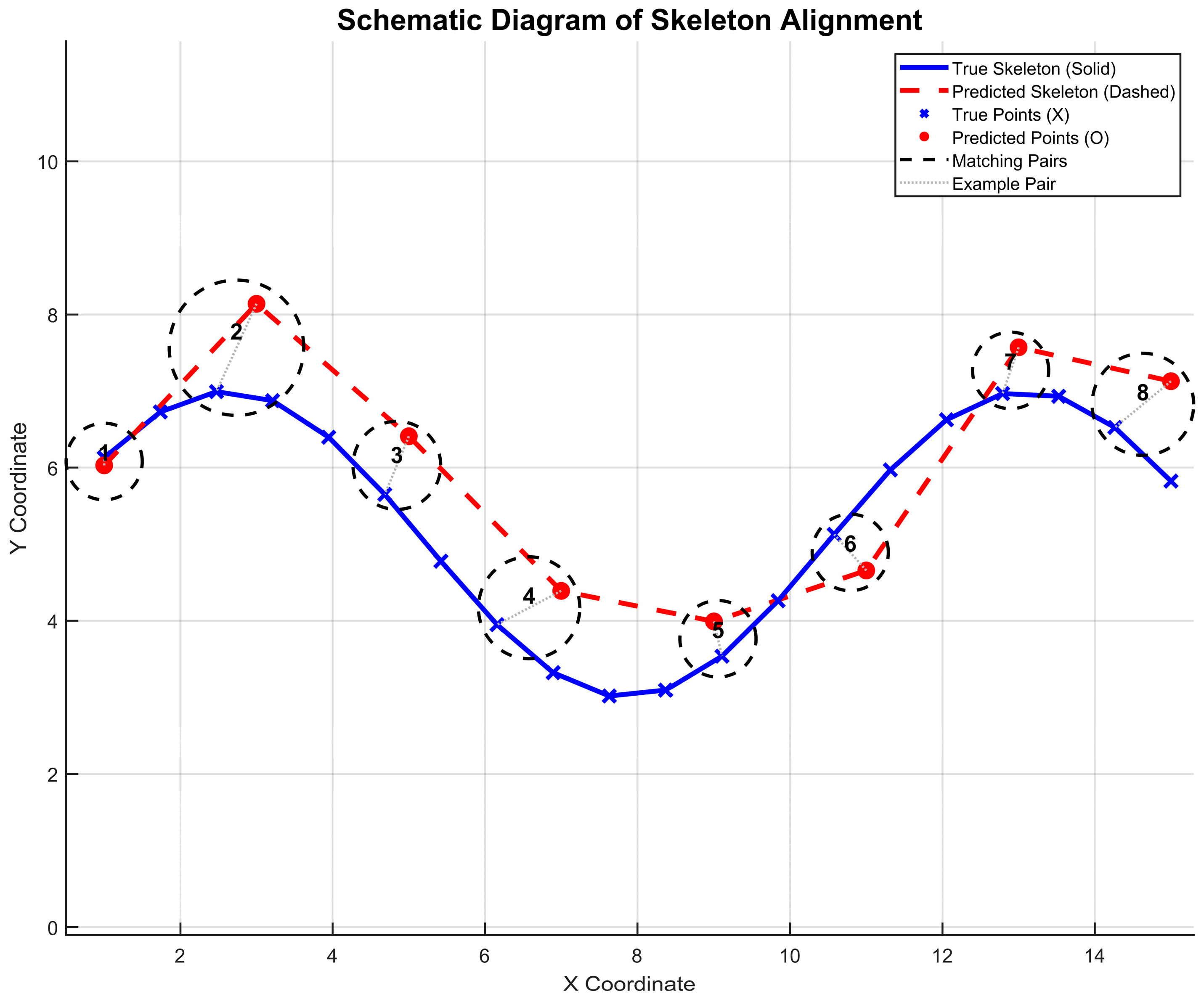
Figure 2. Schematic diagram of skeleton point matching principle.
Buildings 15 03266 g002

2.2. Crack Tip Curvature Radius Error Index (TCRE)

In the field of concrete structure research, the occurrence and propagation of cracks reflect structural safety issues [17,18], while the significant stress concentration at crack tips [19] is a key focus of research attention. Therefore, quantifying and evaluating the identification errors of crack information through the stress concentration effect at crack endpoints holds practical engineering significance. According to fracture mechanics theory, there is a clear negative correlation between the curvature radius of a crack tip and its stress concentration degree: the smaller the curvature radius (i.e., the sharper the tip), the denser the distribution of stress lines in the tip region, and the higher the stress concentration degree; conversely, the larger the curvature radius, the flatter the distribution of stress lines, and the lower the stress concentration degree. This law has been widely verified in studies on quasi-brittle materials such as concrete [20,21,22].
Meanwhile, the double “K” fracture theory further reveals that a smaller curvature radius at the crack tip results in more pronounced stress concentration, which accelerates the crack propagation process [23]. To quantify the difference between the predicted and actual values of the crack tip curvature radius, the tip curvature radius error (TCRE) is introduced. This indicator can more authentically reflect the actual stress distribution characteristics at the crack tip. Figure 3 presents a schematic illustration of the predicted curvature circle results.
The main calculation steps of TCRE in this study are illustrated in Figure 1.
Extraction of crack skeleton endpoints.
First, in the MATLAB environment, the “bwmorph” function is used to extract the crack skeleton, and then the “endpoints” operator of this function is employed to accurately extract the endpoints of the crack skeleton. Subsequently, the “find” function is utilized to obtain the coordinate information of these endpoints, laying the foundation for subsequent calculations.
Selection of ROI (Region of Interest).
Considering issues such as high computational complexity, insufficient targeting, and waste of computing resources when directly calculating the curvature radius for the entire image, this study adopts an ROI definition strategy to focus on the local features of crack skeleton endpoints. When extracting the ROI, the coordinate range is strictly limited, following the principle of covering the key area of the endpoints without exceeding the image boundaries. This not only improves computational accuracy but also significantly reduces the computational load.
Quadratic polynomial fitting and curvature calculation.
For calculating the local curvature at the crack tip, this study selects a five-parameter quadratic polynomial model and uses the nonlinear least squares method to fit the preprocessed ROI data. By minimizing the sum of squared errors between data points and the fitted surface, this method constructs a surface model that can accurately reflect the geometric morphology of the endpoints. The specific MATLAB code is provided in Supplementary Materials (Code A2).
After obtaining the fitting model, a Hessian matrix is constructed based on the fitting results. The eigenvalues of the Hessian matrix are closely related to the principal curvatures of the surface at that point [24]. Principal curvatures reflect the degree of curvature of the surface in different directions, where the eigenvalue with the largest absolute value corresponds to the maximum curvature of the surface and is taken as the curvature at that point. To avoid excessively small curvature values (approaching zero) when the crack tends to be straight, this study sets the lower limit of curvature to 0.00001 (corresponding to a maximum curvature radius of 100,000 pixels). This threshold is determined based on the pixel size and the actual range of crack sizes to ensure the physical rationality and numerical stability of the calculation results. Finally, combined with the pixel size (pixel_size), using Formula (5), the calculated curvature “K” is converted into the actual curvature radius “ ρ “, and the TCR value with physical meaning is obtained.
Z ( x , y ) = a x 2 + b x y + c y 2 + d x + e y + f
H = 2 z x 2 2 z x y 2 z x y 2 z y 2
K = 1 2 λ 1 + λ 2
T C R ( i ) = 1 K S
In the above formula, H denotes the Hessian matrix, λ1 and λ2 are the eigenvalues of the Hessian matrix, K represents the calculated curvature, and S stands for the pixel size.

2.3. Dual-Parameter Error Evaluation Index Weight Setting

The dual-parameter evaluation index proposed in this paper weights the two error indicators (ECWI and TCRE) through weight assignment. The weight values are determined with reference to the relevant provisions on sub-item check coefficients in Article 7.7 of the “Standards for Technical Condition Evaluation of Highway Bridges” (JTG/T H21-2011) [25]. In the existing evaluation system, the formula for the evaluation scale “D” of the bearing capacity check coefficient for masonry and reinforced concrete bridges is shown in Formula (6):
D = j = 1 n a j D j
where a j is the weight value of a certain detection index and satisfies j = 1 3 a j = 1 . D j is the evaluation scale of a certain detection index of a structure or component. The specific weights of each detection index are as follows: 0.4 for defect condition, 0.3 for material strength, and 0.3 for natural vibration frequency. Drawing on this weight system, when weighted-averaging ECWI and TCRE, the weight of the defect condition is assigned to ECWI with a value of 0.4; the mechanical index TCRE, referencing the combined weight of “material strength” and “natural vibration frequency”, is assigned a weight of 0.6. This design ensures that the evaluation results are compatible with the existing specification system, while filling the gap in the precise quantification of evaluation index D j in the specifications, making the evaluation system more comprehensive, scientific, and operable.

3. Model Network Structure and Framework

3.1. MobileNetV2-DeepLabv3+ Model

In this paper, an improved MobileNetV2-DeepLabv3+ model (abbreviated as Mobile-D) is proposed. MobileNetV2 is an efficient neural network architecture that reduces the resource consumption during model operation, while DeepLabv3+ ensures segmentation accuracy. The combination of the two endows the model with significant advantages in deployment on mobile devices and embedded systems [26].
In the early stage of model training, due to reasons such as the insufficient number of parameters in MobileNetV2, the trained Mobile-D suffered from severe overfitting and had inadequate ability to capture the details of concrete cracks. To address this, regularization hyperparameters were configured in the training hyperparameters (see Supplementary Materials (Data B1 for details)): the L2 regularization parameter “L2Regularization” and a piecewise learning rate scheduling strategy that combines “LearnRateSchedule”, “piecewise”, “LearnRateDropFactor”, and “LearnRateDropPeriod”. During the training process, the learning rate is reduced by a specific factor at fixed time intervals to alleviate the overfitting phenomenon.
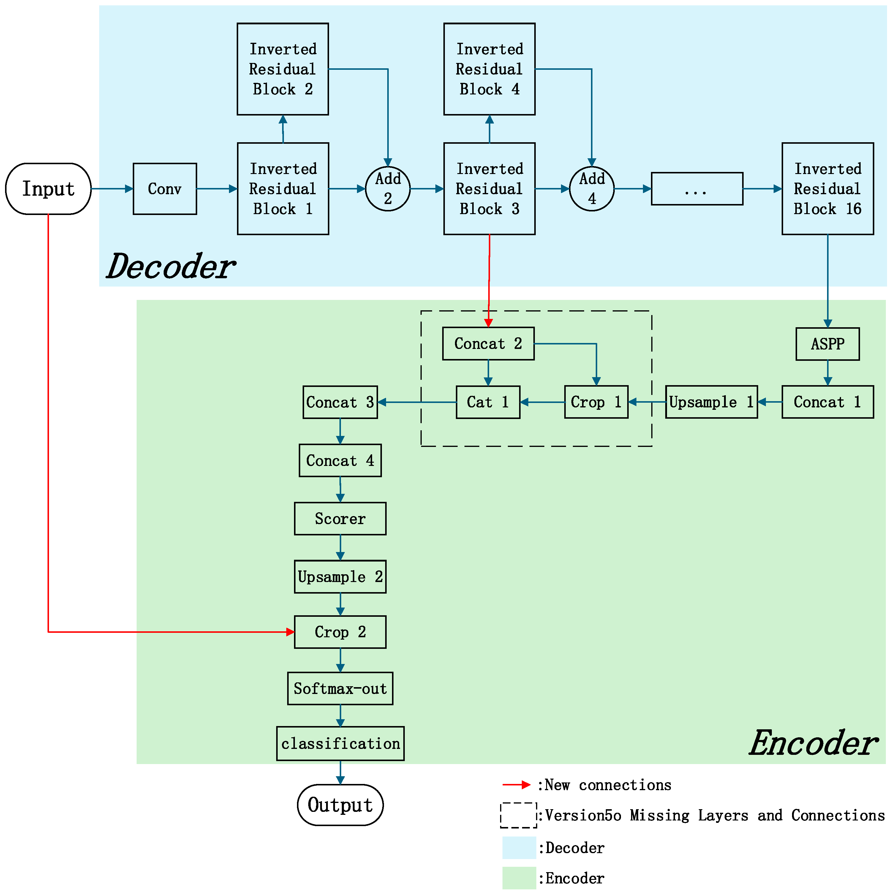
Subsequently, to further tackle overfitting, accurately identify concrete cracks, retain key parameter information such as the initial crack edges and orientations, and avoid the loss of crack details caused by excessive abstraction due to multiple convolution and pooling operations, a connection is added between the expanded convolution activation layer of the inverted residual module in the MobileNetV2 encoder and the decoder.
In order to integrate more original details, priority was given to the inverted residual blocks at the front positions. Since the first and second blocks contained too much noise and the spatial information was significantly lost after the fourth block (with reduced output resolution), while the third inverted residual block had a higher feature map resolution (1/4 of the input size), retained crack edge details, and had a smaller receptive field, which could complement deep features; the third inverted residual block was selected to connect with the decoder for cropping and fusion, as shown in the dashed area in Figure 4. Finally, the input was connected to the decoder and cropped and fused with the feature map output by the up-sample. The newly added connections mentioned above are shown as the red connecting lines in the detailed network structure diagram of Figure 4.
The newly added connection between the expanded convolution activation layer of the third inverted residual block and the concat2 layer of the decoder enables the features extracted by the encoder at this stage to directly participate in feature fusion at a specific stage of the decoder. For concrete crack recognition, the characteristic of this block’s expanded convolution activation layer in increasing feature dimensions and enriching feature representations helps capture the unique feature information of cracks, such as texture and morphology. Introducing these features into the concat2 layer allows the decoder to obtain more comprehensive crack feature information. The enhanced feature integration enables the model to outline the contours of concrete cracks more accurately and improve the accuracy of crack segmentation. To verify the effectiveness of the newly added connection between the extended convolution activation layer of the third inverted residual block and the decoder, an ablation experiment was conducted. The results show that compared with Version5o (without the new connection), Version5 with the new connection generally achieves an improvement in the Dice coefficient by 4.03–26.73%, and the ECWI error index generally decreases by 2.81–6.38%, which verifies the effectiveness of the connection. For detailed comparison of model performance data in the ablation experiment, see Supplementary Materials (Data B2).
Meanwhile, the connection between the input and the cropping layer of the decoder enables low-level detail information such as the color and grayscale of concrete cracks in the original image to directly participate in the decoder for scale matching and fusion with the sampled feature maps. The cropping layer crops the up-sampled feature maps and the original input image to ensure their scales are consistent. This operation effectively adjusts the correlations among features at different scales, assisting the decoder in integrating multi-level information. Consequently, even under complex backgrounds, the model can more accurately identify and segment subtle cracks.

3.2. Training Dataset and Parameter Settings

3.2.1. Training Environment and Dataset

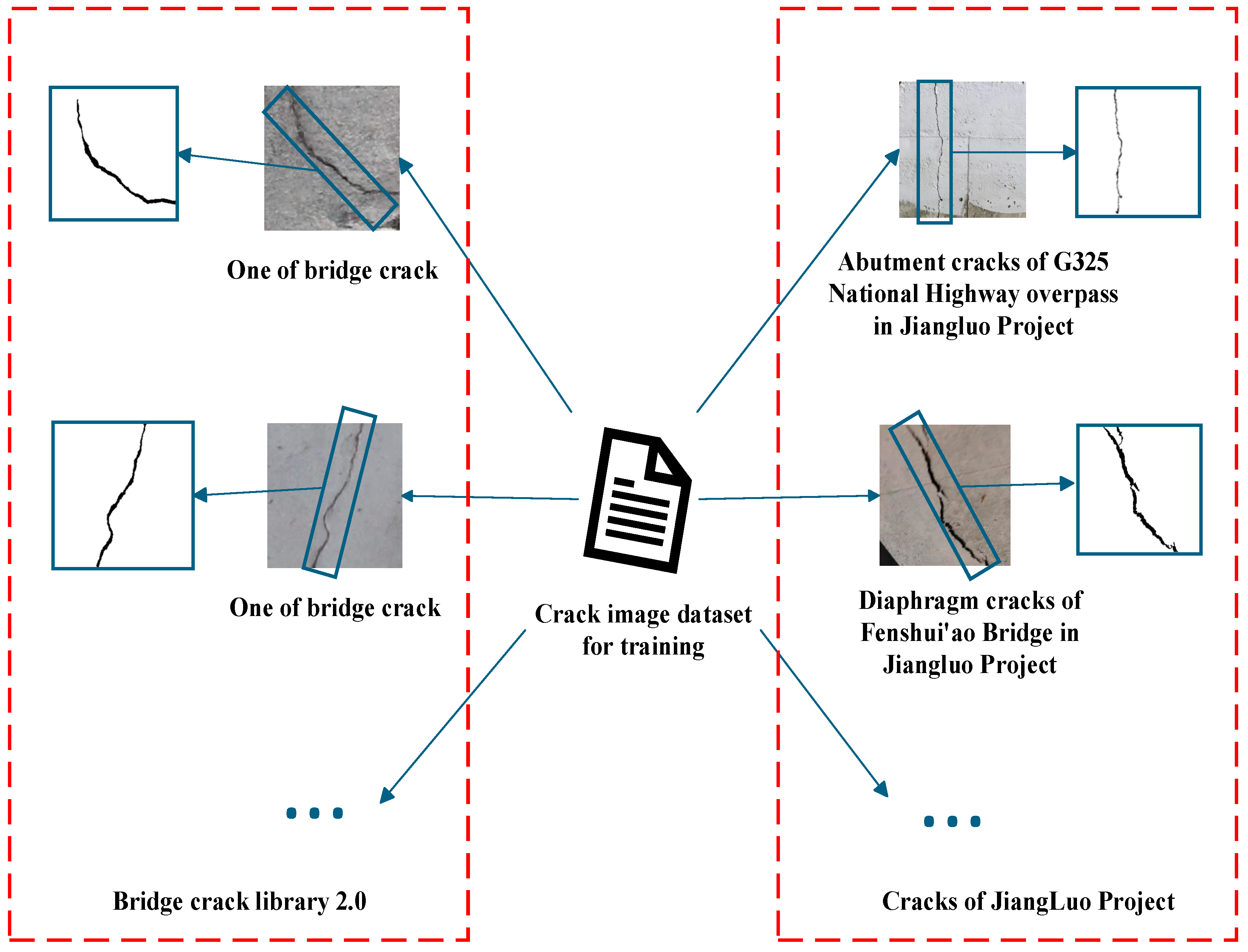
To ensure the validity and comparability of the research, standardized hardware and software environments are used in this study for experiments. An Intel i5-12490F processor, 16 GB running memory, and an NVIDIA RTX 4060 8 GB graphics card (NVIDIA, Santa Clara, CA, USA) are used as the hardware configuration, while model training is completed based on the MATLAB R2022a platform. In terms of data selection, this study selectively adopts the measured crack dataset from the Jiangluo Expressway Project (a sponsored project of this paper) and the open-source dataset Bridge Crack Library 2.0 [27]. All images selected from the Jiangluo Project were collected from the regular bridge inspection reports of the Jiangluo Project bridges in Guangdong Province, China, including Ducun Simply-Supported Hollow Slab Viaduct, National Highway G325 Monolithic Cast-in-Place Continuous Beam Overpass, Shuijing Interchange T-Beam Main Line Bridge, etc. These images cover crack scenarios under the service conditions of bridges, as shown in Figure 5. The dataset consists of approximately 3700 RGB images with a resolution of 256 × 256 pixels, each equipped with accurate binary mask labels; cracks are marked in black (pixel value 0) and the background in white (pixel value 255), facilitating efficient feature recognition by the model. The images are stored in PNG format before cropping, with an average file size of about 5 MB, balancing image clarity and data transmission efficiency. The dataset is divided into a training set, a validation set, and a test set in a ratio of 7:2:1. The test set is applied in the “4 Bridge case” section of this paper.
To optimize the Mobile-D model, comparative numerical experiments were conducted under the new evaluation system through a positive feedback optimization mechanism. By adjusting training parameters, optimizing preprocessing, new versions of the model are developed through training iterations, sorted by iteration time and named Mobile-D-Version1, Mobile-D-Version2… until Mobile-D-Version5. Through the comparison of index results, we explore the optimal training scheme that adapts to the new indexes while achieving high performance.

3.2.2. Training Model Dynamic Weight Setting

Due to the huge gap in the number of pixels between cracks and the background, appropriate weights should be assigned to both during training to enable the model to capture more crack details. For this reason, dynamic class weight calculation is specially set in the model training, and its calculation principle formula is as follows:
W i = c i min ( c 1 , c 2 c n )
c i = 1 f i + ε
where W i represents the normalized class weight, c i denotes the class weight, and f i refers to the pixel frequency of the i -th class. ε is an infinitesimal quantity, which defaults to 2.22 × 10⁻¹⁶ in MATLAB to prevent division-by-zero errors.
For the prediction accuracy of models trained with dynamic weights, current experiments have achieved accuracy comparable to that of fixed weights (1:10) with a Dice difference of <11% and to that of fixed weights (1:20) with a Dice difference of <4%. Meanwhile, it eliminates the cost of manually searching for the optimal weights. The relevant experimental data are shown in Table 2 below, and detailed data can be found in Supplementary Materials Data B3.

3.2.3. Training Hyperparameter Settings

In the iteration from Version 1 to Version 5, training hyperparameters were adjusted from Version 1 to Version 2. Since the ECWI index of Version 1 was generally high (e.g., 110.03% for No. 1 and 105.91% for No. 3), it indicated insufficient accuracy in the model’s localization of crack boundaries. This phenomenon was directly related to the relatively high initial learning rate (InitialLearnRate 0.001) and excessively fast decay rate (LearnRateDropFactor 0.1) of Version 1. A higher initial learning rate might cause the model to be sensitive to noise in the early stages of training, resulting in excessive parameter update amplitudes and difficulty in stably capturing fine-grained features such as cracks. Moreover, the excessively fast decay of the learning rate caused the learning process to stagnate prematurely before the model had fully learned complex cracks, making it impossible to further optimize feature extraction capabilities. Therefore, in Version 2, the InitialLearnRate was reduced from 0.001 to 0.0003 to decrease the initial update intensity and reduce noise interference. Meanwhile, the LearnRateDropFactor was increased from 0.1 to 0.8 to slow down the decay rate, allowing the model sufficient time for iterative optimization on complex samples where Version 1 performed poorly (e.g., images with high ECWI values in No. 1 samples).
The L2Regularization was reduced from 0.0001 to 0.00001, mainly to address the underfitting issue of coarse crack segmentation in Version 1. Reducing the regularization intensity can reduce restrictions on model complexity, enhance the model’s fitting ability to the training set, and enable it to capture more crack details, thereby reducing training loss and improving segmentation accuracy. The GradientThreshold was adjusted from 0.05 to 1 to relax the gradient clipping intensity, releasing the learning potential of the Version 1 model and accelerating model convergence. Finally, the training intensity parameters were appropriately adjusted based on the hardware performance of the training environment.
The comparison of indicators such as ECWI, Dice, and IoU between the two versions is shown in Table 3 below. The overall improvement of indicators including Dice and IoU in the table (except for individual samples) verifies the effectiveness and rationality of the adjustment strategy. For the training hyperparameter settings of Versions 1–5, please refer to Supplementary Materials (Data B1).

3.2.4. Preprocessing and Post-Processing Settings

Preprocessing Settings
To enhance the model’s robustness against geometric deformations, this study performed augmentation on the original data and introduced a new data augmentation function (CustomAugmentation). This function primarily employs two data processing methods: color jittering and elastic deformation [28], achieving multi-modal data augmentation.
(1)
Regarding the settings of color jitter parameters ‘Brightness’, ‘Contrast’, ‘Saturation’, and ‘Hue’, considering that there are no extreme conditions such as excessive light in the dataset, and to improve the model’s robustness against texture interference, we refer to the idea of controlling color jitter intensity in the research on image robustness enhancement by Xu et al. (CVPR 2022 Workshop) [29] and set ‘Brightness’, ‘Contrast’, and ‘Saturation’ to the conservative range [0.8, 1.0]; meanwhile, since the hue of concrete images is stable (without abrupt change characteristics), the ‘Hue’ parameter is set to 0.
(2)
Regarding elastic deformation, the set parameters include the maximum displacement ‘alpha’ and smoothness ‘sigma’. The adjustment of these two parameters during the iterations is shown in Table 4 below.
The specific adjustment approach is based on the model’s predicted result images and the experimental ECWI values and Dice coefficients corresponding to each model version (see Supplementary Materials (Data B1) for the summary table of key performance indicators of Versions 1–5). For instance, in Versions 1 and 2, the predicted cracks were relatively thick, with larger ECWIs and smaller Dice coefficients. Therefore, it was necessary to appropriately reduce the maximum displacement parameter ‘Alpha’ to prevent over-distorted backgrounds caused by an excessively large Alpha from being misjudged as cracks and also appropriately lower the smoothness parameter ‘Sigma’ to alleviate such overfitting and improve generalization ability. The elastic deformation parameters were mainly adjusted from Version 2 to Version 3 and from Version 4 to Version 5.
(3)
Regarding the crack width enhancement part, the width enhancement parameter was introduced starting from Version 4. Since it was observed that the actual crack width varies with shooting distance and lighting conditions (e.g., cracks appear wider in close-up shots), this enhancement was introduced to simulate such physical changes through random scaling. This was to prevent the model from overfitting to cracks of fixed widths and enable it to adapt to cracks of different scales. The dataset was initially set to have a random variation of 0.8–1.2 times (±20%), and this parameter remained unchanged in subsequent version improvements. The data supporting the effectiveness of crack width enhancement is shown in Table 5 below (selected from the summary table in Supplementary Materials Data B1).
Given the randomness and geometric complexity of the branching behavior of concrete cracks, and to address the issue of insufficient branching samples in actual datasets while enhancing the model’s ability to recognize complex crack morphologies, a crack branching simulation function is added prior to training. This simulation strategy draws on the lesion synthesis idea of LesionMix [30]. It enhances the diversity of training data through a random growth algorithm. Additionally, Shorten and Khoshgoftaar [31] have also proposed the effectiveness of synthetic data augmentation in handling complex structures. Regarding the application in bridge structure damage, Minshui Huang et al. [32] adopted the method of expanding a small number of samples with data augmentation to train a steel bridge damage recognition model, which not only enriched the features of training samples but also improved the robustness of the model. It not only effectively alleviates overfitting but also enhances data diversity by simulating structural changes when training data is insufficient in the early stage, thereby compensating for data scarcity. The MATLAB code written by the authors is provided in Supplementary Materials (Code A1).
Post-Processing Settings
It is a significant step to post-process the model’s prediction results for improving segmentation quality, which not only reduces noise interference but also provides a more concise and intuitive comparison for subsequent accuracy evaluation. For the two label categories in the prediction results, “Edge” (crack contours) and “Background”, the post-processing workflow enhances segmentation quality through the following steps:
Binarize the prediction mask: Pixels labeled as “Edge” are set to true, while the rest are set to false.
Optimize the binary mask using morphological operations: First, an opening operation is applied to remove isolated noise and small regions; subsequently, a closing operation is used to connect fragmented target areas, forming more complete edge structures. Finally, connected noise regions with areas smaller than a threshold parameter are further filtered out [33].
Convert the processed binary mask to classification format: Map false and true values to the “Background” and “Edge” categories, respectively. This results in a more precise and distinct segmentation, effectively improving the reliability of model predictions. The detailed post-processing workflow is illustrated in Figure 6.

3.2.5. Selection of Loss Functions

The loss function is the “core feedback tool” in the training of recognition models (such as image classification, semantic segmentation, etc.). Its core role is to measure the gap between the model’s prediction results and the real situation and then timely correct the model parameters through backpropagation during the training process so that the model can be optimized towards convergence. The weighted cross-entropy hybrid loss function adopted in this paper is a classic method for addressing class imbalance issues in the field of semantic segmentation and is particularly suitable for the detection of slender targets such as cracks. For example, Chen, C. et al. [34] mixed the Dice Loss function with the original cross-entropy loss function and conducted experiments on road crack datasets. The results showed that the mIoU of the model using only the original cross-entropy loss function could only reach 66.43%, while the combination of cross-entropy, DiceLoss and FocalLoss achieved 68.15%. It can be seen that the combination of cross-entropy and Dice Loss plays the most significant role in improving the recognition effect of the model, verifying the effectiveness of the weighted cross-entropy loss. Fan Haokun, Liu Xiangyang et al. [35] proposed ST-UNet for the low-brightness characteristics of concrete cracks, which adopted Focal+Dice hybrid loss, leading to a 22% increase in IoU and a 17% increase in Dice. Hong Jun, Liu Xiaonan et al. [36] combined cross-entropy loss function and Dice loss function to solve the problem of target class imbalance in street scenes. On the street scene datasets Cityscapes and CamVid, the mean intersection over union (mIoU) of the model was increased by 3.9% and 3.0% respectively compared with the traditional U-Net network.
The hybrid loss function employed in this paper incorporates an edge-aware weighting mechanism. Specifically, the Sobel operator is used to extract edge information for generating edge masks, with the loss weights of edge regions enhanced accordingly. In addition to edge weighting, the loss function also integrates the crack weights described in Section 3.2.2 to address the class imbalance issue. The overall loss is calculated as the average cross-entropy loss over the entire batch. Figure 7 presents the flowchart of the loss function processing system. The detailed implementation code is provided in Supplementary Materials (Code A3).

4. Bridge Case

4.1. ECWI Experimental Results

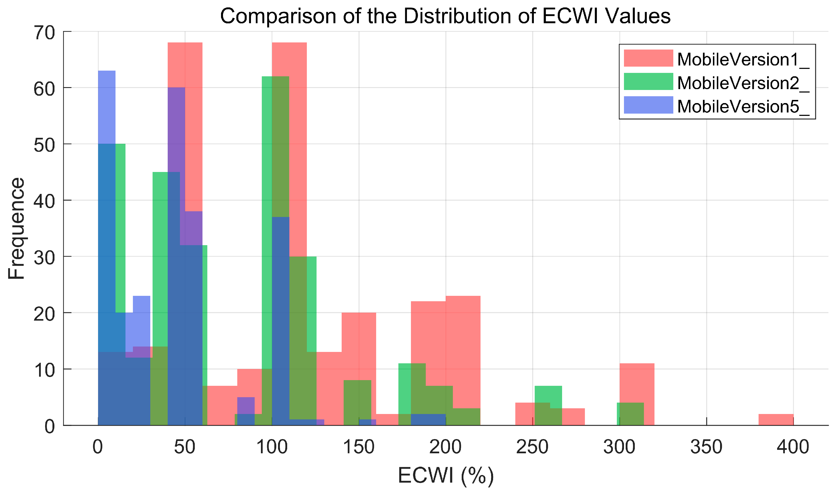
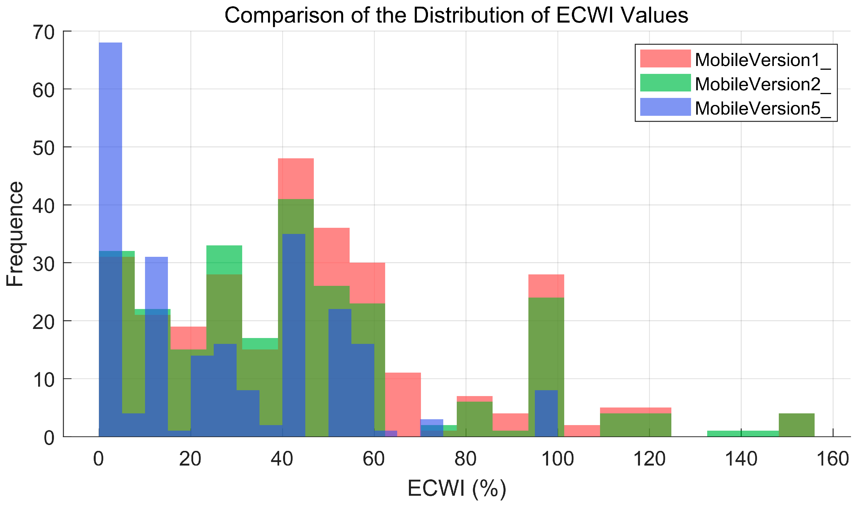
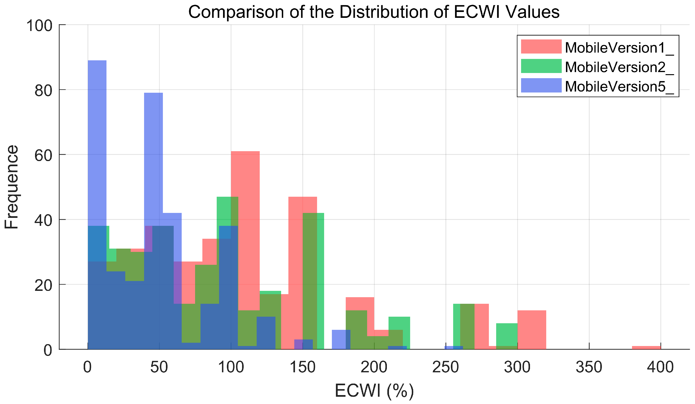
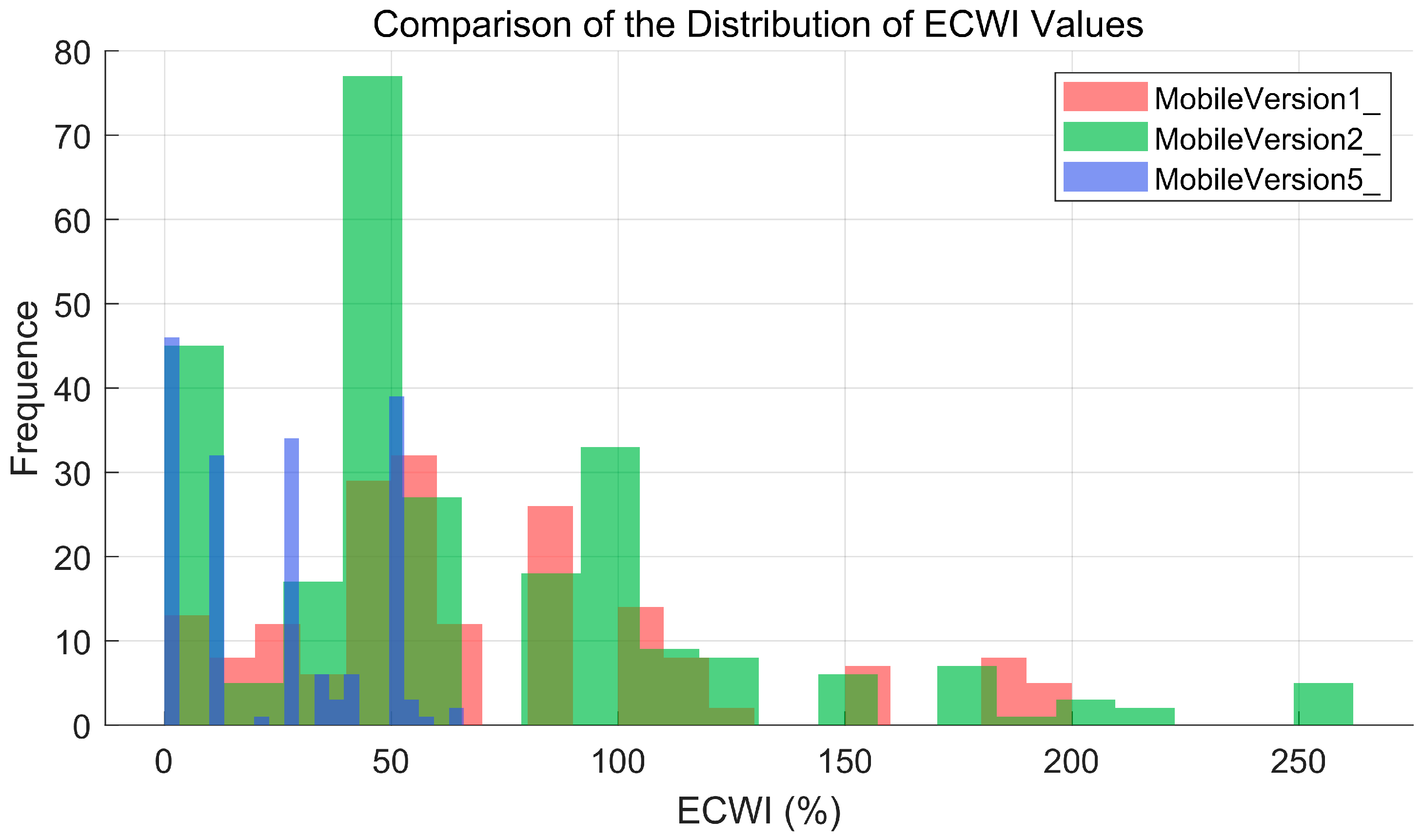
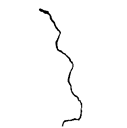
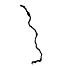
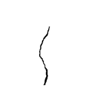
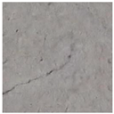
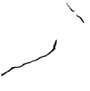
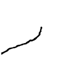
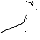
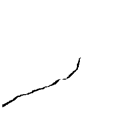
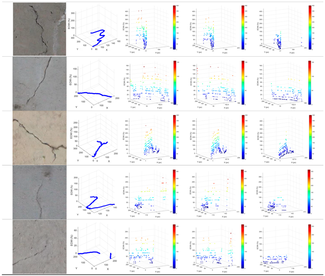
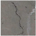
The data of the test set in this experiment is derived from the test set divided in Section 3.2.1 of this paper, from which five samples were selected for verification and comparison. The results are presented in the form of black-and-white binary images (see Table 6), combined with 3D heatmaps (Table 7) and histogram analyses (Figure 8, Figure 9, Figure 10, Figure 11 and Figure 12).
From the 3D heatmap (Table 7), the spatial distribution of predicted crack error magnitudes across different crack locations can be observed. Among these, the model prediction results where error points exhibit a “sinking” distribution pattern are considered superior.
In the debugging and optimization of the Mobile-D model, significant improvements were achieved in the ECWI detection of the same validation sample by adjusting the elastic deformation parameters of the crack branching simulation function, the geometric constraint conditions of the post-processing function, the width control parameters, and the edge weight parameters of the classification layer.
Through a comparison of overall prediction results across version iterations, compared with Mobile-D-Version1, the error distribution in the medium-error region of Mobile-D-Version2 has been optimized, with most prediction points falling into the low-error region. For example, in Figure 10, the bar for Mobile-D-Version2 (green) in the error range [150%, 200%] is lower than that of Mobile-D-Version1 (red). The ECWI of Mobile-D-Version5 has significantly decreased. As observed in Table 7 and Table 8, for the same validation sample, the proportion of prediction points in the medium-error region is below 3%; even for samples No. 2 and No. 5, there are no prediction points in the medium-error region, with 99% of prediction points concentrated in the low-error region (blue). Analysis of the histogram further shows that over 40% of ECWI values fall within the [0, 25%] range. Additionally, statistical data in Table 8 indicates that the average ECWI of Mobile-D-Version5 has dropped to less than 50% of that of Mobile-D-Version1.

4.2. TCRE Experimental Results

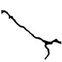
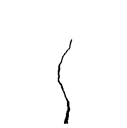
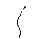
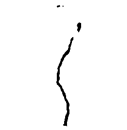
The current version has been optimized through training up to the fifth iteration, namely, Mobile-D-Version5. Among them, the prediction results of the Mobile-D-Version1, Mobile-D-Version2, and Mobile-D-Version5 models on the same validation sample are shown in Table 9. The samples cover diverse crack tip morphologies: the curvature radii range from 0.10 mm to 1.24 mm (including 0.10 mm, 0.26 mm, 0.27 mm, 0.49 mm, 1.24 mm, etc.), encompassing both sharp tips (small curvature) and blunt tips (medium curvature), thus covering typical crack tip scenarios commonly seen in engineering. Samples No. 2 and No. 3 are temporarily excluded from the experimental results because their crack labels have no obvious endpoints. The percentage errors in the table are calculated before rounding, which may differ from the rounded values presented in the table. The values in parentheses represent the calculated curvature radius, with the unit being millimeters (mm).
Based on the statistical analysis results of TCRE, among the three valid samples (samples No. 2 and No. 3 were not included in the curvature radius analysis due to missing crack endpoint labeling data), the predicted curvature radius values of the Mobile-D model generally tend to be smaller. According to the inference mentioned in Section 3.2 of this paper—that a decrease in curvature radius will lead to an increase in the structural stress concentration degree—this prediction characteristic exhibits a certain degree of rationality from the perspective of engineering safety redundancy [37,38].
As indicated in Table 9 of TCRE prediction results, in terms of evaluating the prediction stability of the models, when comparing Mobile-D-Version1 and Mobile-D-Version2, the former exhibits greater volatility in TCRE prediction, with poorer stability of prediction errors than the latter. The Mobile-D-Version1 model exhibits obvious sample dependence: when processing simple crack morphologies (e.g., sample No. 5), the prediction error can be as low as 1.5%; however, when faced with complex crack endpoint features (e.g., sample No. 1), the error rises sharply to 74.3%; even samples No. 6 and No. 8 reach 309.8%. This shows that the initial version of the model has insufficient sensitivity and generalization ability to complex geometric features. By appropriately adjusting the training hyperparameters, Mobile-D-Version2 has stably controlled the fluctuation range of prediction errors for most samples within 30%. The TCRE stability of Mobile-D-Version5 has been further improved compared with Mobile-D-Version2.

4.3. Weighted Comprehensive Comparison

Against the background of emphasizing the hazards of stress concentration, a weighted comprehensive evaluation of the two indicators (ECWI and TCRE) is conducted using a weight ratio of 4:6, with specific results shown in Table 10. This evaluation method fully reflects the key role of weight allocation in the comprehensive assessment of the model.
As shown in Table 10, when the crack recognition model identifies samples No. 1 to No. 5, the corresponding ECWI values decrease with the upgrade of the model version. This indicates a significant reduction in geometric recognition errors, reflecting the optimization of the intelligent recognition model’s ability to identify crack geometric shape parameters. Combined with Table 9, although the TCRE values of each sample did not show a significant downward trend with the training optimization of versions, the cohesion and stability of TCRE values have improved significantly as the version number of the recognition model has increased. This suggests that the performance of the recognition model tends to be stable with training optimization, and its robustness has been significantly enhanced. In the comprehensive weighted evaluation, from Version 1 to Version 5, the recognition error of sample No. 1 decreased from 88.59% to 28.39%, that of sample No. 4 decreased from 40.50% to 28.57%, and that of sample No. 5 decreased from 28.22% to 20.00%. The overall error shows a downward trend, reflecting the optimization of the model in capturing details of structural cracks.

4.4. Experiments on SDNET2018 Datasets

To test the robustness and universality of the model, the open-source dataset SDNET2018 [39] was selected for verification. Ten images were extracted from the dataset based on features such as crack orientation and distribution location and verified using the Version 5 model. The core accuracy index data of the verification are shown in the following Table 11.
As can be seen from the data in Table 11 above, the average Dice coefficient is 0.7893, with the minimum Dice coefficient being 0.6307, and most of them are 0.7 or even 0.8. The average ECWI is 23.856%, with the minimum being 11.48% and the maximum being 35.47%. It can be concluded that the model exhibits good cross-dataset recognition ability, high recognition similarity, strong capability in capturing detailed features of cracks, as well as favorable universality and robustness.

5. Conclusions

(1)
In terms of model optimization, an efficient error positive feedback optimization mechanism is established, which is applicable not only to the Mobile-D model but also to other semantic segmentation models. Through the dual-parameter comprehensive evaluation system, in-depth analysis and feedback on the detection results are conducted. Based on the analysis results, the training parameters, preprocessing function parameters, etc. are dynamically adjusted to carry out a new round of iterative training. By continuously optimizing model parameters, this mechanism effectively improves the prediction accuracy and generalization ability of the model, ensuring that the model can still maintain excellent performance in complex detection scenarios. Furthermore, when the model is applied to other datasets, its robustness and universality still perform excellently.
(2)
A creative geometric–mechanical dual-parameter evaluation method for crack recognition errors is proposed. Through qualitative analysis of TCRE on the key influencing factors of stress concentration errors at crack tips, the cross-disciplinary evaluation index is constructed by weighted averaging of ECWI and TCRE to assess the prediction accuracy of crack semantic segmentation models. This evaluation method complements traditional performance accuracy metrics (such as the Dice coefficient and IoU intersection ratio), enabling it to provide experimenters with a comprehensive evaluation from multiple professional perspectives. The evaluation of ECWI and TCRE can provide error references for the assessment of items related to crack defects in the bearing capacity deterioration coefficient mentioned in Article 7.7.4 [16] of the “Specification for Inspection and Evaluation of Load-bearing Capacity of Highway Bridges” (JTG/T J21-2011) in bridge inspection work. By quantifying errors generated in the detection process, it effectively reduces interference from human judgment and improves the objectivity and accuracy of bridge inspection work.
(3)
In terms of algorithm research, this study conducted an in-depth exploration of the implementation and optimization processes of the TCRE algorithm and ECWI algorithm. Not only was the automation of the calculation process initially realized, but through code function development, the function of outputting visualized comparison results of indicators was integrated into the algorithm code, achieving a high level of overall code integration.
(4)
Based on the above analysis, the current model system still has issues such as high dispersion in prediction results and poor adaptability to complex samples. In subsequent research, consideration will be given to introducing an attention mechanism module to enhance the model’s ability to perceive the curvature radius characteristics of crack endpoints, optimize the trend-capturing capability of the prediction algorithm, and thereby improve the model’s prediction accuracy and stability. Regarding model training, the optimal training configurations, such as the parameters for color jitter and elastic deformation in data augmentation, crack training weights, and training hyperparameters, still need to be further optimized and improved. For the dual-parameter evaluation system, its weighted weight values are selected in accordance with existing standards, which have certain engineering statistical significance and strong applicability. However, from the perspective of academic research, combined with model characteristics and practical applications, there is still room for optimization of this weight. In addition, the current application of TCRE only serves as a preliminary assessment of the safety of crack prediction models, and the specific mathematical relationship between TCRE and the stress field requires further in-depth research.

Supplementary Materials

The following supporting information can be downloaded at: https://www.mdpi.com/article/10.3390/buildings15183266/s1.

Author Contributions

Conceptualization, and methodology, K.P. and W.W.; software, W.W.; validation, K.P. and W.W.; resources, K.P.; writing—original draft preparation, K.P. and W.W.; writing—review and editing, K.P.; supervision, K.P.; project administration, K.P.; funding acquisition, K.P. All authors have read and agreed to the published version of the manuscript.

Funding

This research was funded by Guangdong Province Highway Construction Co., Ltd. Affiliated Project, grant number (2022-Company affiliated 026) and 2023 Guangdong Province Graduate Education Innovation Program Project (2023ANLK_081).

Data Availability Statement

The data that has been used is available.

Conflicts of Interest

The authors declare no conflicts of interest.

References

  1. Zhao, T.Q.; Gou, H.Y.; Chen, X.Y.; Li, W.; Liang, H.; Chen, Z.; Zhou, S. Research progress of bridge informatization and intelligent bridges in 2020. J. Civ. Environ. Eng. (Chin. Engl.) 2021, 43, 268–279. [Google Scholar]
  2. Araya-Santelices, P.; Grande, Z.; Atencio, E.; Lozano-Galant, J.A. Bridge management with AI, UAVs, and BIM. Autom. Constr. 2025, 175, 106170. [Google Scholar] [CrossRef]
  3. Ma, T.; Xiao, F.; Zhang, C.; Zhang, J.; Zhang, H.; Xu, K.; Luo, X. Digital twin for 3D interactive building operations: Integrating BIM, IoT-enabled building automation systems, AI, and mixed reality. Autom. Constr. 2025, 176, 106277. [Google Scholar] [CrossRef]
  4. Sarfarazi, S.; Shamass, R.; Guarracino, F.; Mascolo, I. Exploring the stainless-steel beam-to-column connections response: A hybrid explainable machine learning framework for characterization. Front. Struct. Civ. Eng. 2025, 19, 34–59. [Google Scholar] [CrossRef]
  5. Deng, Z.; Huang, M.; Wan, N.; Zhang, J. The Current Development of Structural Health Monitoring for Bridges: A Review. Buildings 2023, 13, 1360. [Google Scholar] [CrossRef]
  6. Le-Xuan, T.; Nguyen-Chi, T.; Bui-Tien, T.; Tran-Ngoc, H. ResUNet4T: A potential deep learning model for damage detection based on a numerical case study of a large-scale bridge using time-series data. Eng. Struct. 2025, 340, 120668. [Google Scholar] [CrossRef]
  7. Huang, M.; Zhang, J.; Hu, J.; Ye, Z.; Deng, Z.; Wan, N. Nonlinear modeling of temperature-induced bearing displacement of long-span single-pier rigid frame bridge based on DCNN-LSTM. Case Stud. Therm. Eng. 2024, 53, 103897. [Google Scholar] [CrossRef]
  8. Huang, C.P.; Tian, W.Y.; Li, Q. Research on quantitative identification method of concrete bridge defects based on U-Net and mathematical morphology. Bridge Constr. 2025, 55, 64–71. [Google Scholar] [CrossRef]
  9. Ritzy, R.; Umadevi, V.A.; Girija, K.; Rajan, R. Binary-class concrete surface crack detection using a transfer learning model. Knowl.-Based Syst. 2025, 324, 113953. [Google Scholar] [CrossRef]
  10. Su, M.; Wan, J.; Zhou, Q.; Wang, R.; Xie, Y.; Peng, H. Utilizing pretrained convolutional neural networks for crack detection and geometric feature recognition in concrete surface images. J. Build. Eng. 2024, 98, 111386. [Google Scholar] [CrossRef]
  11. Inglis, C.E. Stresses in a plate due to the presence of cracks and sharp corners. Trans. Inst. Naval Archit. 1913, 55, 219–241. [Google Scholar]
  12. Huang, M.; Wan, N.; Zhu, H. Reconstruction of structural acceleration response based on CNN-BiGRU with squeeze-and-excitation under environmental temperature effects. J. Civil. Struct. Health Monit. 2025, 15, 985–1003. [Google Scholar] [CrossRef]
  13. Wan, C.; Zhou, Z.; Li, S.; Ding, Y.; Xu, Z.; Yang, Z.; Xia, Y.; Yin, F. Development of a Bridge Management System Based on the Building Information Modeling Technology. Sustainability 2019, 11, 4583. [Google Scholar] [CrossRef]
  14. JTG/T 3310-2019; Code for Durability Design of Concrete Structures in Highway Engineering. China Communications Press Co., Ltd.: Beijing, China, 2019.
  15. JTG 5120-2021; Specifications for Maintenance of Highway Bridges and Culverts. China Communications Press Co., Ltd.: Beijing, China, 2021.
  16. JTG/T J21-2011; Specification for Inspection and Evaluation of Load-bearing Capacity of Highway Bridges. China Communications Press Co., Ltd.: Beijing, China, 2011.
  17. Shu, J.; Zhang, Z.; Gonzalez, I.; Karoumi, R. The application of a damage detection method using Artificial Neural Network and train-induced vibrations on a simplified railway bridge model. Eng. Struct. 2013, 52, 408–421. [Google Scholar] [CrossRef]
  18. Shu, J.; Honfi, D.; Plos, M.; Zandi, K.; Magnusson, J. Assessment of a cantilever bridge deck slab using multi-level assessment strategy and decision support framework. Eng. Struct. 2019, 200, 109666. [Google Scholar] [CrossRef]
  19. Dong, W.; Wu, Z.; Tang, X.; Zhou, X. A comparative study on stress intensity factor-based criteria for the prediction of mixed mode I-II crack propagation in concrete. Eng. Fract. Mech. 2018, 197, 217–235. [Google Scholar] [CrossRef]
  20. Ince, R. Using SCB specimens to quantify nonlinear fracture characteristics in concrete and rock materials. Eng. Fract. Mech. 2025, 318, 110951. [Google Scholar] [CrossRef]
  21. Cisowski, A.; Kowalik, M.P. The influence of the cross-sectional geometry on stress concentration in 3D printed concrete elements: A preliminary study. Eng. Struct. 2025, 340, 120728. [Google Scholar] [CrossRef]
  22. Zhang, B.; Luo, Z.; Yan, L.; Zhang, Y.; Wang, Z.; Yang, Q.; Li, J. Study on the influence mechanism of polypropylene fiber on crack propagation of concrete with existing cracks under uniaxial compression. Theor. Appl. Fract. Mech. 2024, 131, 104429. [Google Scholar] [CrossRef]
  23. Xu, S.; Reinhardt, H. Determination of double-K criterion for crack propagation in quasi-brittle fracture, Part II: Analytical evaluating and practical measuring methods for three-point bending notched beams. Int. J. Fract. 1999, 98, 151–177. [Google Scholar] [CrossRef]
  24. Langenfeld, K.; Kurzeja, P.; Mosler, J. On the curvature dependence of gradient damage models: Control and opportunities. Comput. Methods Appl. Mech. Eng. 2023, 410, 115987. [Google Scholar] [CrossRef]
  25. JTG/T H21-2011; Standards for Technical Condition Evaluation of Highway Bridges. China Communications Press Co., Ltd.: Beijing, China, 2011.
  26. Sandler, M.; Howard, A.; Zhu, M.; Zhmoginov, A.; Chen, L. Mobilenetv2: Inverted residuals and linear bottlenecks. In Proceedings of the 2018 IEEE/CVF Conference on Computer Vision and Pattern Recognition (CVPR), Salt Lake City, UT, USA, 18–23 June 2018; pp. 4510–4520. [Google Scholar]
  27. Jin, T.; Ye, X.W.; Li, Z.X. Establishment and evaluation of conditional GAN-based image dataset for semantic segmentation of structural cracks. Eng. Struct. 2023, 285, 116058. [Google Scholar] [CrossRef]
  28. Sun, D.; Dornaika, F.; Charafeddine, J. LCAMix: Local-and-contour aware grid mixing based data augmentation for medical image segmentation. Inf. Fusion 2024, 110, 102484. [Google Scholar] [CrossRef]
  29. Xu, Y.; Mou, C.; Hu, Y.; Xie, J.; Zhang, J. Robust Invertible Image Steganography. In Proceedings of the IEEE/CVF Conference on Computer Vision and Pattern Recognition (CVPR), New Orleans, LA, USA, 18–24 June 2022; pp. 7875–7884. [Google Scholar]
  30. Pan, X.; Chen, M.; Lin, H.; Bian, X.; Feng, S.; Chen, J.; Wang, L.; Chen, X.; Liu, Z.; Lan, R. LesionMix data enhancement and entropy minimization for semi-supervised lesion segmentation of lung cancer. Appl. Soft Comput. 2024, 167 Pt A, 112244. [Google Scholar] [CrossRef]
  31. Shorten, C.; Khoshgoftaar, T.M. A survey on Image Data Augmentation for Deep Learning. J. Big Data 2019, 6, 60. [Google Scholar] [CrossRef]
  32. Huang, M.; Zhang, J.; Li, J.; Deng, Z.; Luo, J. Damage identification of steel bridge based on data augmentation and adaptive optimization neural network. Struct. Health Monit. 2024, 24, 1674–1699. [Google Scholar] [CrossRef]
  33. Printemps, T.; Dabertrand, K.; Vives, J.; Valery, A. Application of a novel local and automatic PCA algorithm for diffraction pattern denoising in TEM-ASTAR analysis in microelectronics. Ultramicroscopy 2024, 267, 114059. [Google Scholar] [CrossRef]
  34. Chen, C.; Sun, X.; Long, H.; Hao, X. Pavement crack detection method based on improved DeepLabv3+ network. Semicond. Optoelectron. 2024, 45, 493–500. [Google Scholar] [CrossRef]
  35. Fan, H.-K.; Liu, X.-Y. Concrete Crack Detection Based on ST-UNet and Target Features. Comput. Syst. Appl. 2024, 33, 77–84. [Google Scholar]
  36. Hong, J.; Liu, X.; Liu, Z. Semantic segmentation of street view images by fusing attention and multi-scale features. Comput. Syst. Appl. 2024, 33, 94–102. [Google Scholar]
  37. Fang, Z.X.; Fan, H.T. Redundancy of Structural Systems in the Context of Structural Safety. Procedia Eng. 2011, 14, 2172–2178. [Google Scholar] [CrossRef]
  38. Möller, N.; Hansson, S.O. Principles of engineering safety: Risk and uncertainty reduction. Reliab. Eng. Syst. Saf. 2008, 93, 798–805. [Google Scholar] [CrossRef]
  39. Maguire, M.; Dorafshan, S.; Thomas, R.J. SDNET2018: A Concrete Crack Image Dataset for Machine Learning Applications; Utah State University: Logan, UT, USA, 2018. [Google Scholar] [CrossRef]
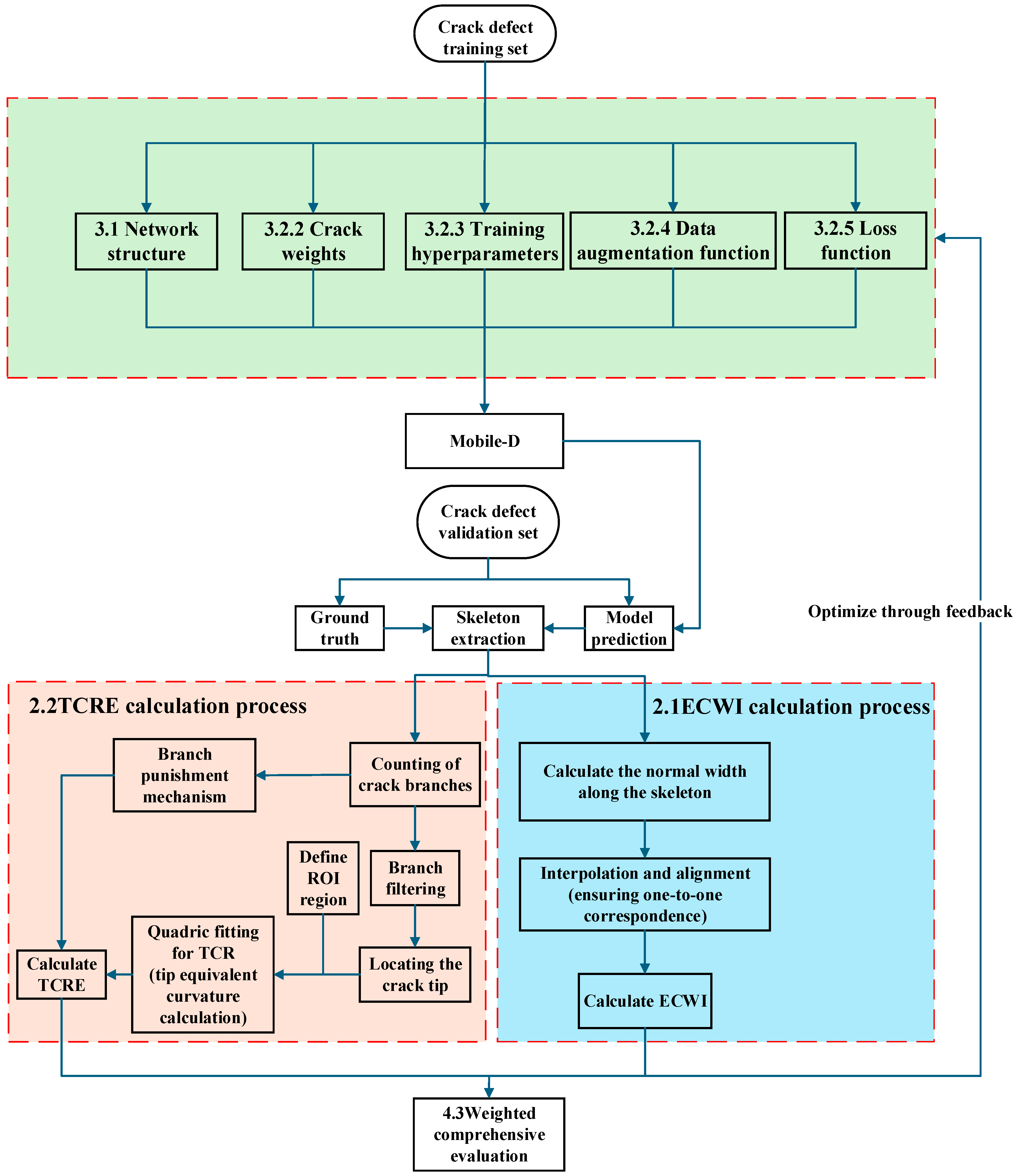
Figure 1. Flowchart of dual-parameter error evaluation system for bridge concrete crack segmentation.
Buildings 15 03266 g001
Figure 3. Curvature circle prediction result diagram.
Buildings 15 03266 g003
Figure 4. Network structure diagram of the Mobile-D Model.
Buildings 15 03266 g004
Figure 5. Composition of training data.
Buildings 15 03266 g005
Figure 6. Post-processing flowchart.
Buildings 15 03266 g006
Figure 7. Flowchart of loss function processing.
Buildings 15 03266 g007
Figure 8. Histogram of error comparison for prediction results of crack No. 1.
Buildings 15 03266 g008
Figure 9. Histogram of error comparison for prediction results of crack No. 2.
Buildings 15 03266 g009
Figure 10. Histogram of error comparison for prediction results of crack No. 3.
Buildings 15 03266 g010
Figure 11. Histogram of error comparison for prediction results of crack No. 4.
Buildings 15 03266 g011
Figure 12. Histogram of error comparison for prediction results of crack No. 5.
Buildings 15 03266 g012
Table 1. Detailed data of cracks (part).
Serial NumberX-CoordinateY-CoordinatePredicted Width (px)Actual Width (px)
183184.005.66
284182.835.66
385182.004.47
486194.005.66
587194.005.66
688204.475.66
789205.666.32
Table 2. Weight experiment comparison table.
Crack ImageWeightDiceIoUPAECWI
No. 11:100.75620.60800.992434.05%
1:200.72690.57100.991932.14%
Dynamic weight0.71590.55750.990840.38%
No. 21:100.86520.76250.995317.47%
1:200.84970.73860.995118.34%
Dynamic weight0.84980.73880.994626.37%
No. 31:100.77250.62930.986148.87%
1:200.76380.61790.986536.24%
Dynamic weight0.74920.59890.985047.58%
No. 41:100.82510.70230.996420.70%
1:200.79660.66200.995920.45%
Dynamic weight0.79410.65860.995728.38%
No. 51:100.75930.61200.993225.91%
1:200.70870.54880.992124.37%
Dynamic weight0.68660.52270.992524.50%
Table 3. Comparison table of performance indicators (Versions 1–2).
Crack ImageVersionDiceIoUPAECWI
No. 1Version 10.64190.47270.9838110.03%
Version 20.70200.54080.987988.69%
No. 2Version 10.64150.47220.981547.59%
Version 20.66650.49980.983544.69%
No. 3Version 10.70530.54470.9783105.91%
Version 20.71250.55340.979296.33%
No. 4Version 10.67250.50660.990279.05%
Version 20.70240.54130.991668.07%
No. 5Version 10.66350.49640.988368.31%
Version 20.59420.42270.983565.15%
Table 4. Table of elastic deformation parameter adjustments (Versions 1–5).
VersionAlphaSigma
Version 1105
Version 2105
Version 355
Version 455
Version 533
Table 5. Comparison table of performance indicators (Versions 3–4).
Crack ImageVersionDiceIoUPAECWI
No. 1Version 30.65200.48360.984648.4%
Version 40.73620.58260.991121.13%
No. 2Version 30.75370.60480.989148.21%
Version 40.84800.73610.994427.37%
No. 3Version 30.69390.53130.9769108.94%
Version 40.74350.59170.984845.34%
No. 4Version 30.75820.61060.993560.51%
Version 40.80370.67180.995829.90%
No. 5Version 30.70760.54750.990750.59%
Version 40.67360.50780.992326.12%
Table 6. Comparison chart of model prediction results.
ImageLabelMobile-D-Version1Mobile-D-Version2Mobile-D-Version5
Buildings 15 03266 i001Buildings 15 03266 i002Buildings 15 03266 i003Buildings 15 03266 i004Buildings 15 03266 i005
Buildings 15 03266 i006Buildings 15 03266 i007Buildings 15 03266 i008Buildings 15 03266 i009Buildings 15 03266 i010
Buildings 15 03266 i011Buildings 15 03266 i012Buildings 15 03266 i013Buildings 15 03266 i014Buildings 15 03266 i015
Buildings 15 03266 i016Buildings 15 03266 i017Buildings 15 03266 i018Buildings 15 03266 i019Buildings 15 03266 i020
Buildings 15 03266 i021Buildings 15 03266 i022Buildings 15 03266 i023Buildings 15 03266 i024Buildings 15 03266 i025
Table 7. Thermal comparison diagram of model prediction results.
LabelMobile-D-Version1Mobile-D-Version2Mobile-D-Version5
Buildings 15 03266 i026
Table 8. Error density distribution table.
Low-Error Region [1, 150] (%)Medium-Error Region [150, 400] (%)High-Error Region [400, 400+] (%)Average ECWI (%)
1Mobile-D-Version167.17%32.83%0.00%110.03%
Mobile-D-Version282.31%17.69%0.00%88.69%
Mobile-D-Version598.83%1.17%0.00%40.38%
2Mobile-D-Version198.64%1.36%0.00%47.59%
Mobile-D-Version298.83%1.17%0.00%44.69%
Mobile-D-Version5100.00%0.00%0.00%26.37%
3Mobile-D-Version170.78%28.92%0.00%105.91%
Mobile-D-Version273.84%26.16%0.00%96.33%
Mobile-D-Version596.68%3.32%0.00%47.58%
4Mobile-D-Version183.17%16.83%0.00%79.05%
Mobile-D-Version286.15%13.85%0.00%68.07%
Mobile-D-Version599.43%0.57%0.00%28.38%
5Mobile-D-Version189.01%10.99%0.00%68.31%
Mobile-D-Version290.87%9.13%0.00%65.15%
Mobile-D-Version5100.00%0.00%0.00%24.50%
Table 9. Statistical table of TCRE calculation results.
Sample NumberPixel Image of SampleTip Curvature RadiusMobile-D-Version1Mobile-D-Version2Mobile-D-Version5
1Buildings 15 03266 i027(0.53)(0.93)
74.3%
(0.70)
30.3%
(0.43)
20.4%
4Buildings 15 03266 i028(0.23)(0.19)
14.8%
(0.17)
26.7%
(0.16)
28.7%
5Buildings 15 03266 i029(0.36)(0.35)
1.5%
(0.25)
30.9%
(0.42)
17.0%
6Buildings 15 03266 i030(0.10)(0.30)
207.0%
(0.18)
87.6%
(0.12)
27.5%
7Buildings 15 03266 i031(0.26)(0.35)
34.8%
(0.33)
27.5%
(0.20)
22.4%
8Buildings 15 03266 i032(0.49)(2.02)
309.8%
(0.60)
22.2%
(0.36)
26.8%
9Buildings 15 03266 i033(1.24)(2.69)
116.9%
(0.52)
58.3%
(0.59)
52.4%
10Buildings 15 03266 i034(0.27)(0.61)
125.6%
(0.43)
59.1%
(0.42)
54.1%
Table 10. ECWI, TCRE evaluation table.
Sample NumberModel VersionECWITCREWeighted Comprehensive Evaluation Error (4:6)
1Mobile-D-Version1110.03%74.3%88.59%
Mobile-D-Version288.69%30.3%53.66%
Mobile-D-Version348.4%41.8%44.44%
Mobile-D-Version421.13%48.5%37.55%
Mobile-D-Version540.38%20.4%28.39%
2Mobile-D-Version147.59%
Mobile-D-Version244.69%
Mobile-D-Version348.21%
Mobile-D-Version427.37%
Mobile-D-Version526.37%
3Mobile-D-Version1105.91%
Mobile-D-Version296.33%
Mobile-D-Version3108.94%
Mobile-D-Version445.34%
Mobile-D-Version547.58%
4Mobile-D-Version179.05%14.8%40.50%
Mobile-D-Version268.07%26.7%43.25%
Mobile-D-Version360.51%12.8%31.88%
Mobile-D-Version429.90%34.0%32.36%
Mobile-D-Version528.38%28.7%28.57%
5Mobile-D-Version168.31%1.5%28.22%
Mobile-D-Version265.15%30.9%44.60%
Mobile-D-Version350.59%20.5%32.54%
Mobile-D-Version426.12%47.7%39.07%
Mobile-D-Version524.50%17.0%20.00%
Note: For the crack samples No. 2 and No. 3 in the table, the tip could not be detected to calculate TCRE because there were no crack endpoints or the crack endpoints had not been fully collected.
Table 11. SDNET2018 prediction results table.
ImageBuildings 15 03266 i035Buildings 15 03266 i036Buildings 15 03266 i037Buildings 15 03266 i038Buildings 15 03266 i039
LabelBuildings 15 03266 i040Buildings 15 03266 i041Buildings 15 03266 i042Buildings 15 03266 i043Buildings 15 03266 i044
PrecisionBuildings 15 03266 i045Buildings 15 03266 i046Buildings 15 03266 i047Buildings 15 03266 i048Buildings 15 03266 i049
Dice0.70220.84720.84460.84850.7848
ECWI33.43%14.29%12.41%22.63%33.83%
ImageBuildings 15 03266 i050Buildings 15 03266 i051Buildings 15 03266 i052Buildings 15 03266 i053Buildings 15 03266 i054
LabelBuildings 15 03266 i055Buildings 15 03266 i056Buildings 15 03266 i057Buildings 15 03266 i058Buildings 15 03266 i059
PrecisionBuildings 15 03266 i060Buildings 15 03266 i061Buildings 15 03266 i062Buildings 15 03266 i063Buildings 15 03266 i064
Dice0.72880.85410.82830.63070.8238
ECWI35.47%28.44%11.48%12.95%33.63%
Disclaimer/Publisher’s Note: The statements, opinions and data contained in all publications are solely those of the individual author(s) and contributor(s) and not of MDPI and/or the editor(s). MDPI and/or the editor(s) disclaim responsibility for any injury to people or property resulting from any ideas, methods, instructions or products referred to in the content.