Article

Fragility Analysis of Prefabricated RCS Hybrid Frame Structures Based on IDA

by
Yuliang Wang
1,2,
Guocan Sun
1,
Xuyue Wang
1,2,*,
Xinyue Zhang
1 and
Czesław Miedziałowski
3
1
School of Civil Engineering, Tianjin Chengjian University, Tianjin 300384, China
2
Tianjin Key Laboratory of Civil Structure Protection and Reinforcement, Tianjin 300384, China
3
Department of Building Structures and Structural Mechanics, Faculty of Civil Engineering and Environmental, Bialystok University of Technology, 15-351 Bialystok, Poland
*
Author to whom correspondence should be addressed.
Buildings 2025, 15(17), 3207; https://doi.org/10.3390/buildings15173207
Submission received: 5 August 2025 / Revised: 27 August 2025 / Accepted: 3 September 2025 / Published: 5 September 2025

Abstract

The prefabricated reinforced concrete columns–steel girder (RCS) hybrid frame structure using column–column connections is a kind of green and environmentally friendly building structure; its seismic performance is investigated. The seismic susceptibility and key influencing factors are systematically evaluated through the establishment of an analytical model and incremental dynamic analysis (IDA) method. A typical three-span, six-story prefabricated RCS hybrid frame structure is designed and numerically modeled with good agreement with the test data. Sa(T1,5%) and PGA double ground motion intensity parameters are selected for IDA analysis. A comparison between the quantile curve method and the conditional logarithmic standard deviation method reveals that using Sa(T1, 5%) as the intensity measure (IM) provides greater reliability for analyzing the vulnerability of the prefabricated RCS hybrid frame structure. The seismic probability demand model of the structure is fitted with Sa(T1,5%) as a parameter and the seismic fragility curves of the structure are plotted; this shows that the slope of the seismic fragility curves becomes smaller after the structure enters the elastic–plastic state, and exhibits good seismic performance. By studying the effects of concrete strength, longitudinal reinforcement strength, and the axial compression ratio on the seismic fragility, it can be seen that with the increase in concrete strength and longitudinal reinforcement strength, and the decrease in axial compression ratio, the overall ductility of the structure increases, the resistance to lateral deformation of the RCS hybrid frame structure is enhanced, and the seismic performance of the prefabricated structure is improved.

1. Introduction

Earthquakes, as highly destructive disasters, are frequent and serious in China. Seismic fragility analysis has become an important seismic design method by evaluating the seismic performance of structures through quantitative analysis [1], in which incremental dynamic analysis (IDA) can effectively evaluate the seismic capacity [2]. As an innovative system integrating precast concrete columns and steel girders, prefabricated reinforced concrete columns–steel girder (RCS) is efficiently assembled through standardized nodes [3]. Its core advantage lies in the complementary material properties, in which concrete columns provide compressive stability and fire resistance, while steel girders play a role in lightweight, large-span and high ductility. At the same time, it significantly improves the construction efficiency and optimizes the seismic performance, and is therefore more efficient and environmentally friendly [4,5] than the traditional cast-in-place concrete frames. In view of the high density of cities in China’s high-seismicity zones, it is of urgent practical significance to carry out research on the seismic mechanism and optimization of the design of this structural system to improve the seismic capacity of buildings and realize green and safe construction.
Many scholars have deepened their knowledge of RCS structures through experiments and numerical simulations. Si et al. [6] proposed a seismic method and applied it to six-story prefabricated RCS frames and verified the practicability of the method through elastic analysis. Murari et al. [7] evaluated the seismic performance of different RCS frames through nonlinear analyses. Dai et al. [8] established that the overall seismic performance of a steel web beam–RC tube–column hybrid structural system can meet the seismic design requirements for high intensity earthquakes through testing. Ghezeljeh et al. [9]’s IDA fragility assessment confirms that RCS frames exhibit 35% higher collapse capacity than RC systems with stable displacement performance, while steel frames show superior strength–ductility but require 14% greater seismic intensity for collapse initiation. Men et al. [10] by novel hybrid RCS frames with seismic fuses achieve targeted reparability via a dual-parameter design, validating functional recovery acceleration through optimized fuse components. Pan et al. [11] validate that prefabricated RCS joints meet a strong column–weak beam hierarchy with flag-shaped hysteresis by cyclic testing. Cai et al. [12] studied in depth the seismic performance of RCS frame specimens under different nodal connection types by establishing finite element models.
IDA as a method to study seismic performance was first proposed by Bertero [13], and then further studied by Vamvatsikos and Cornell [2,14]. The steps of IDA analysis [15] first need to establish the relevant model, select the seismic wave that meets the site conditions, and determine the appropriate IM (Seismic motion intensity index, Intensity Measure, IM for short) and DM (Damage index, Damage Measure, DM for short), perform amplitude to modulate the intensity of seismic waves and input the seismic wave step by step into the structure for time course analysis. Single-record IDA curves and multiple-record IDA curve clusters are constructed, followed by quantile regression analysis of the IDA clusters to plot the conditional logarithmic standard deviation of the IM with respect to the DM.
For IDA, scholars have carried out several studies. Cheng et al. [16] confirm that concentrated low-frequency spectral content significantly elevates collapse probability by IDA seismic analysis of high-rises subject to long-period ground motions. Jouneghani et al. [17] study the IDA-based seismic performance assessment of Elliptic Braced Frames, and establish as critical seismic design criteria for this innovative structural system. Fanaie et al. [18] conducted an IDA-based assessment of steel frames with pioneering fragility curves enabling building damage evaluation. Wu et al. [19] found that the IDA of RECCs (Engineered Cementitious Composites) frames validates superior seismic deformation capacity versus RC systems. Ren et al. [20] through IDA analysis of seven RC frames established by SAP2000 found that concrete strength inversely correlates to damage probability and axial compression ratio increases structural vulnerability. Li et al. [21] found that the reserve capacity of the CBF (concentrically braced frames) contributes appreciably to collapse prevention, and IDA-derived collapse ductility spectra are more suitable for assessing the collapse of CBFs with dynamic instability. Xu et al. [22] carried out a machine learning (ML)-based seismic response prediction for RC frames comparison of the IDA method. IDA fragility analysis of concrete-filled square tubular (CFST) frames by Liu et al. [23] confirms 6–16% higher vulnerability in spatial frames under multi-directional excitation versus planar systems. Qiu et al. [24] proposed a method to quantitatively evaluate the structural ductility based on IDA.
Additionally, compared to a conventional all-RC frame, the RCS system combines steel beams with concrete columns, offering greater ductility and energy dissipation capacity, which significantly enhances seismic performance. Meanwhile, whereas traditional RC frames are prone to brittle failure and slow construction, the prefabricated RCS solution also improves construction speed and quality control through modular connections. Furthermore, the prefabricated approach simplifies the complex on-site construction of joints, resulting in more stable and reliable structural performance.
At present, there are more studies on the fragility of cast-in-place RCS frame structures and fewer studies on the fragility of prefabricated frame structures and even fewer on column–column joints. These studies are still in the primary stage, and the relevant theoretical system has not been perfected. In view of this, this study aims to systematically analyze the seismic fragility performance of a prefabricated RCS hybrid frame through the development of an integrated structural model using column–column connections and the application of the IDA method. IDA-based seismic fragility analyses were carried out under different influencing factors, including concrete strength, longitudinal reinforcement strength, and axial compression ratio, using both Sa and PGA as ground motion intensity measures. The results are intended to provide academic reference for further research on the seismic behavior of new prefabricated structural systems.

2. Frame Structure Model Design

2.1. Model Validation

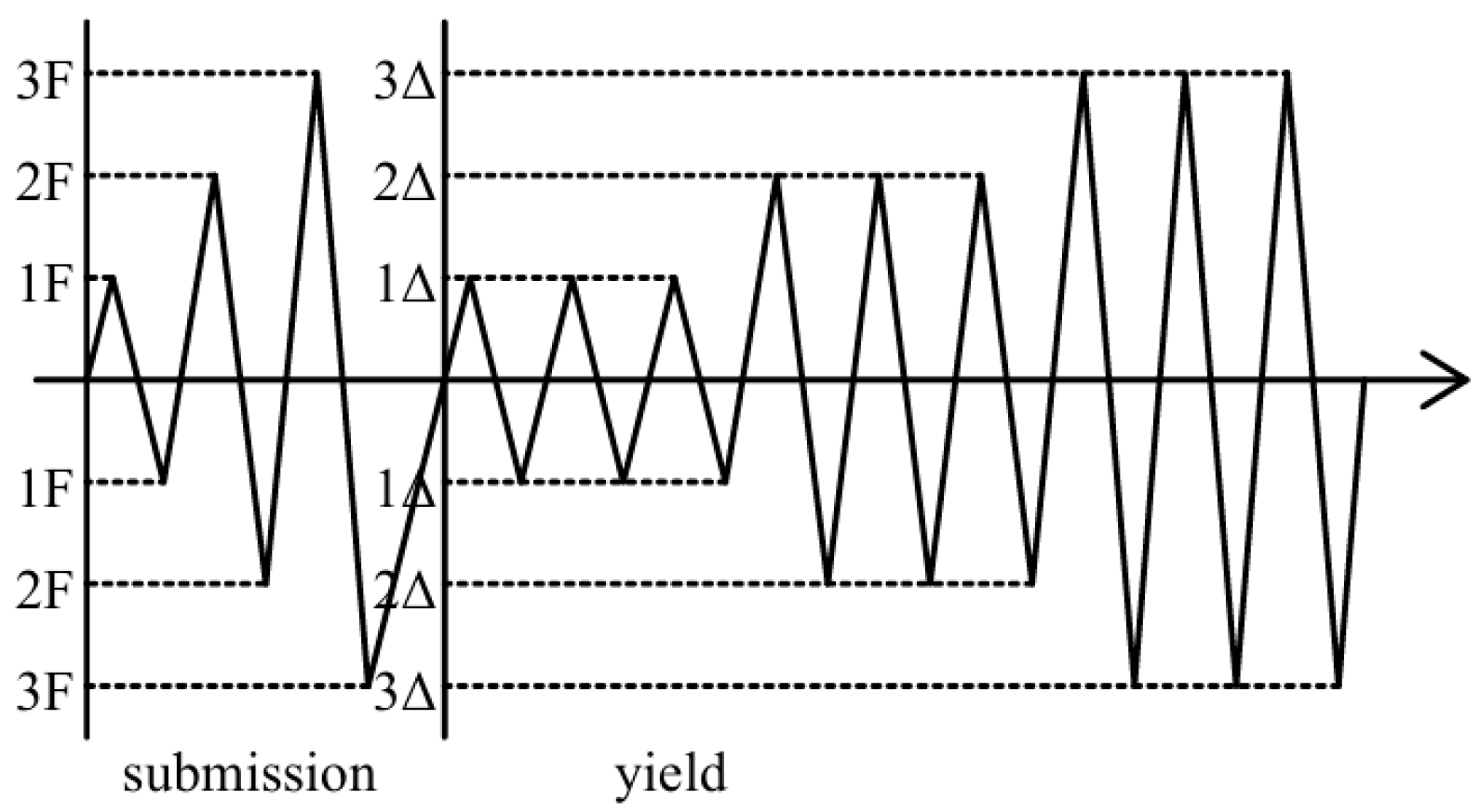
In order to ensure the validity of the established column–column connection joint model, the PRCC-01 (Prefabricated Reinforced Concrete Column) specimen in the literature [25] is simulated and the reasonableness is verified by comparing the main characteristic values of the numerical model with the test results. The cross-section size of the assembled column specimen is 400 mm × 400 mm (the length and the width are equal), the concrete strength grade is C40, and the thickness of the concrete protection layer is 20 mm. The specimen information is shown in Table 1. The specimen was subjected to a low-cycle reciprocating pseudo-static test, and the test loading device and the corresponding lateral loading protocol are shown in Figure 1 and Figure 2.
The column–column connection joint model is established by SAP2000 Base Version, and the dimensions of each part of the model are the same as those of the test specimen. The connection unit is set in the middle of the assembled column, and the fixed-end support is used at the bottom end of the column. Figure 3 is the established column–column connection joint model. In the finite element model, the constitutive model for concrete is employed using the Mohr–Coulomb model, while the constitutive model for steel adopts the Von Mises yield criterion, with a bilinear kinematic hardening model utilized to simulate its elastoplastic behavior.
By comparing the simulation and experimental results, the hysteresis curves comparison is presented in Figure 4, where the black segments represent the measured load-displacement hysteresis responses, while the red segments indicate the simulated data from this study. The differences in ultimate load are summarized in Table 2. The results demonstrate that the numerical model more accurately captures the characteristics of the joint, and the simulation outcomes show close agreement with the experimental data, validating the rationality of the numerical model.

2.2. Establishment of the Prefabricated RCS Hybrid Structure Model

According to the current seismic design code in China [26], a six-story, three-span prefabricated RCS hybrid frame structure with a floor height of 3.6 m is designed. The seismic fortification intensity is 8 degrees, the design seismic grouping is Group II, the site category is Class II, and the structural feature period is Tg = 0.40 s. For the elastic–plastic time–history analysis of a rare earthquake, a damping ratio of 5% is used. The concrete slab is 120 mm thick, the floor dead load value is 5.0 kN/m2, the live load is 2.0 kN/m2, the constant load value of the non-accessible roof is 7.0 kN/m2, and the live load is 0.5 kN/m2. The prefabricated RCS hybrid structure model is established by SAP2000 Base Version software as shown in Figure 5a. The structural side facade and floor plan are shown in Figure 5b,c.
All the frame steel beams in the structure are selected as H400 × 146 × 14.5 × 14.5 (mm), and the strength grade of steel is Q345. The column cross-section size is 600 × 600 (mm), the strength grade of the column concrete is C40, the longitudinal reinforcement is HRB400, and the stirrup is HRB335. The reinforcement of the column cross-section is obtained using PKPM V1.4 structural design software, as shown in Figure 5d. The results of the structural vibration model period are shown in Table 3. From Table 3, it can be seen that the periods of the structural vibration modes have not exceeded the specified limits 0.9 [27], indicating that the structure meets the code requirements under seismic action.

3. Simulation Results and Analysis

3.1. IDA Analysis

3.1.1. IDA Analysis Under a Single Ground Vibration

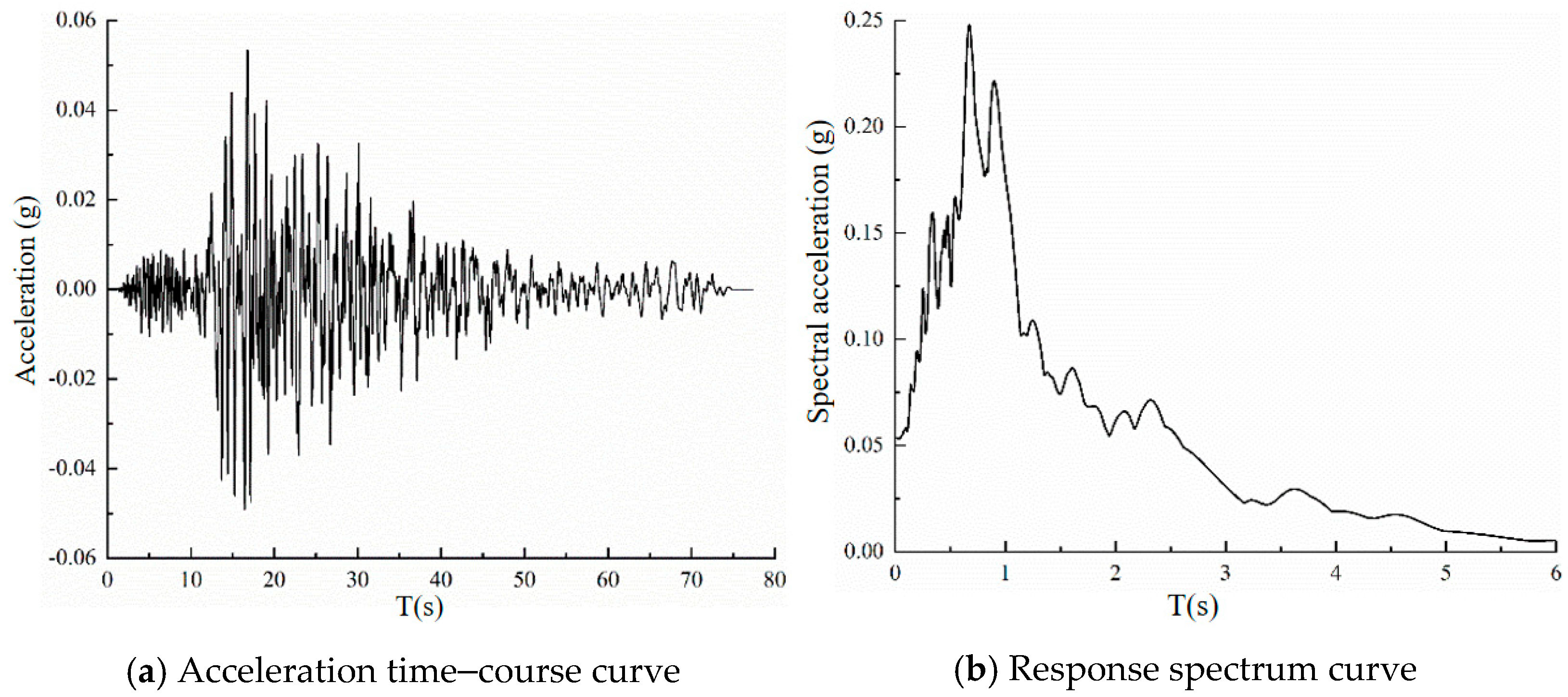
Based on the site classification of the construction location, peak ground acceleration or intensity was considered, and identical or similar station records were selected as input. After selecting the ground motions, the influence of the response spectrum plateau and the site predominant period were also taken into account. All models in this study were designed for an intensity of 8 degrees, a site Class II, with an equivalent shear wave velocity Vse ranging from 250 to 500 m/s. Kern County waves measured at the Pasadena-CIT Athenaeum site were selected for incremental dynamic analysis of the structure. The acceleration time–course curve of Kern County wave is shown in Figure 6a. The response spectrum curve of Kern County wave was calculated by using Seismosignal v2021 software with a damping coefficient of 5%, as shown in Figure 6b. Two indicators of ground motion intensity, Sa(T1,5%) (spectral acceleration, Sa for short) and PGA (peak ground acceleration, abbreviated as PGA), were used to plot the IDA curves.
Through the modal analysis of the building structural model, the fundamental period of the structural model is obtained as T1 = 0.7767 s, and the response spectral acceleration Sa(T1,5%) = 0.1866 g corresponding to the first period of the structure with a damping ratio of 5% can be obtained from Figure 6b. For the incremental dynamic analysis of the structure, the amplitude modulation step is taken as 0.4 g, and the increment of the step is taken as 0.05 g, and for the first analysis, taken Sa(T1,5%) = 0.05 g, its amplitude modulation coefficient at this time is λ1 = 0.05/0.1866 = 0.2680. The hunt and fill algorithm [28] is used to perform the amplitude modulation of the seismic recordings. Starting from the second analysis, the formula for calculating Sa(T1,5%) is: San = San−1 + amplitude scaling interval (0.4 g) + (n − 2) × step increment (0.05 g) where n represents the sequence number (n ≥ 2).
For example:
When n = 2, Sa2 = 0.05 g + 0.4 g + (2 − 2) × 0.05 g = 0.45 g
When n = 3, Sa3 = 0.45 g + 0.4 g + (3 − 2) × 0.05 g = 0.90 g
and so on. Refer to Table 4 for details.
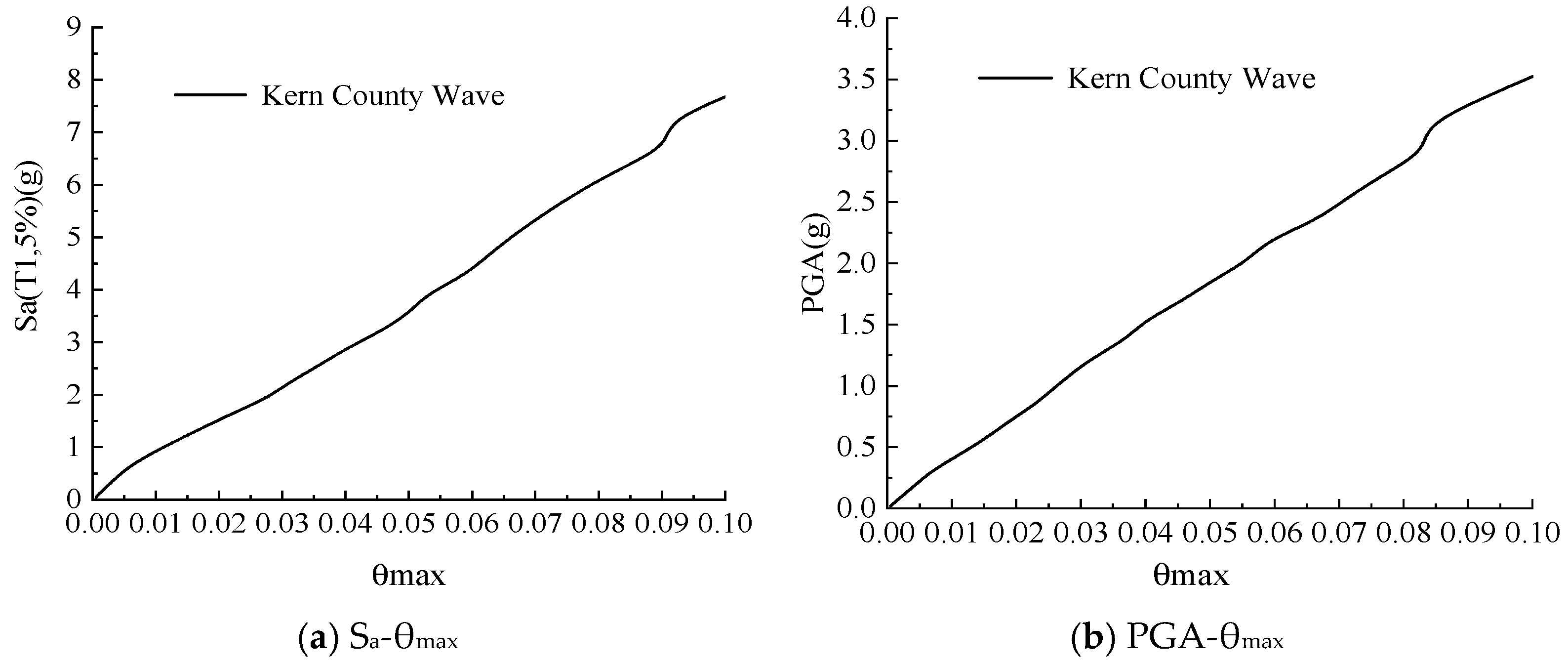
By using the amplitude-modulated Kern County wave 24 times for time–procedure analysis, obtaining a variety of different reference points, each set of reference points was constructed on the DM-IM coordinate system, and the IDA curves were finally obtained through linear interpolation, as shown in Figure 7.
As can be seen from Figure 7, the structure is in the elastic stage when the ground vibration is small, and the two IDA curves are growing linearly. When the interlayer displacement angle θmax is close to 0.005, the structure enters into the yielding stage, and the slope appears to be decreasing. We then continue to carry out IDA analysis on the structure and it is terminated until the θmax reaches 0.1. At this time, the curve does not form an obvious decline section. On the contrary, there is a local slope increase and even a “hardening stage”, “torsional response”, and “re-strengthening” which cause this undesirable phenomenon to arise. This phenomenon is affected by the type of structure [29], and also has a certain relationship with the selection of seismic waves, the effective duration of seismic waves [30], and the loading direction [31] and other factors.

3.1.2. IDA Analysis Under Multiple Ground Vibration

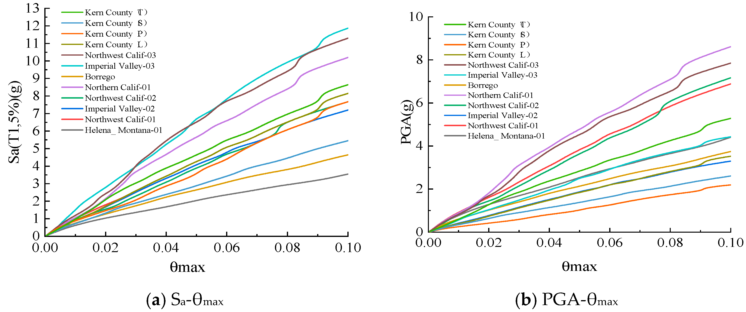
For the prefabricated RCS hybrid frame structure in this paper, it is not enough to consider the effect of only 1 seismic wave, so 12 seismic waves collected from the literature [20] are used and the IDA curve clusters are obtained by the IDA method, as shown in Figure 8. It can be seen that the damage to the structure under different ground motion intensities varies greatly. It is affected by different seismic motion intensity indicators. The dispersion of the IDA curve clusters also shows relatively large differences.
The dispersion of the IDA curve clusters reflects the uncertainty inherent in structural seismic responses. To further investigate the primary factors contributing to this uncertainty, this study draws on the feature importance analysis method from the field of machine learning. Kazemi et al. [32] through machine learning analysis of extensive reinforced concrete structural data, explicitly identified the spectral acceleration Sa(T1), fundamental structural period, and number of stories as the three most critical parameters for predicting seismic responses, with significantly higher importance scores than other factors.

3.1.3. IDA Curve Cluster Statistics and Analysis

Two methods, the quantile method [33] and the conditional logarithmic standard deviation method, were used to plot the result curve of the two parameters, Sa(T1,5%) and PGA, respectively. The aim is to determine the ground motion indicators which are more suitable for seismic fragility analysis.
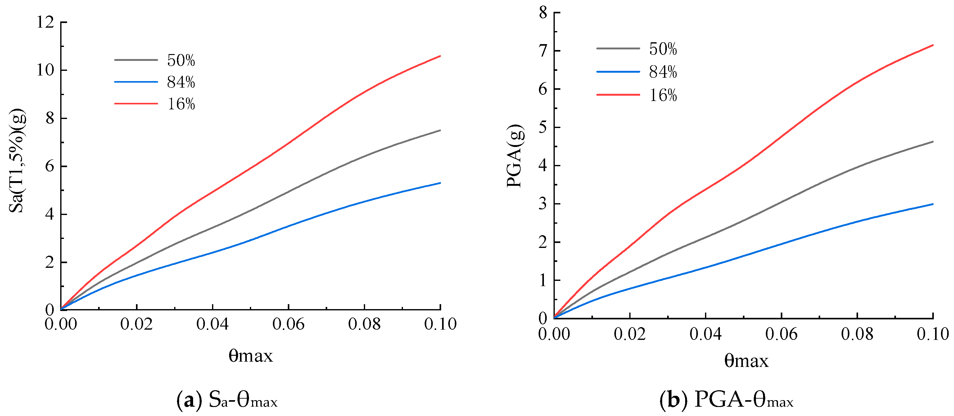
For the quantile method, the principle of DM (in this paper, the maximum interlayer displacement angle is chosen as DM) is used for the discrete data statistics firstly. Under the same index of structural damage, μ is derived for all IM values using Equation (1), and all logarithmic standard deviations δ are obtained using Equation (2). Finally, three curves are obtained in the coordinates of D M , μ ,     D M , μ × e + δ , and D M , μ × e δ corresponding to the IDA quantile curves of 50%, 16%, and 84%, respectively. The quantile curves are shown in Figure 9. Equations (1) and (2) are as follows:
μ = exp n ln x i / n
δ = n ln x i ln x i 1 2 / n 1 1 / 2
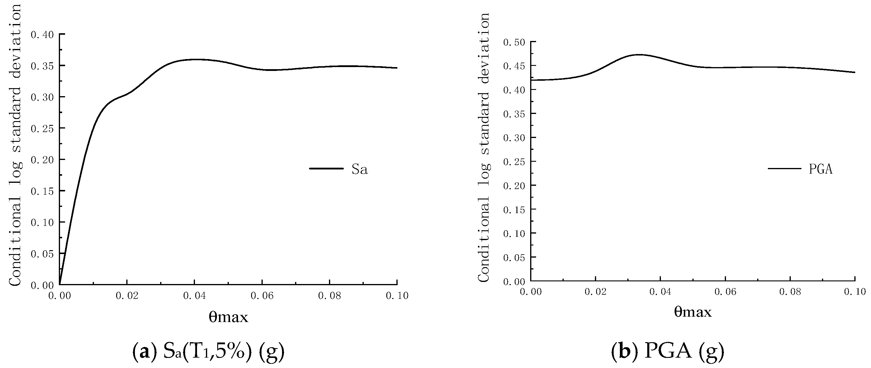
Based on a comparison of the quantile curves, it has been observed that when Sa(T1,5%) is adopted as the intensity measure, the structural damage indicator exhibits reduced deviation, while the IDA curves demonstrate lower dispersion and higher reliability. Since the ground motion intensity index under the structural damage index condition conforms to the lognormal distribution, the mean quantification of the conditional logarithmic standard deviation σ ln I M / D M of IM relative to DM is compared to analyze the discretization under the two-parameter condition. Figure 10 shows the conditional logarithmic standard deviation curve under the two parameters. As shown in Figure 10, the mean value of the conditional logarithmic standard deviation based on PGA is significantly higher than that of Sa(T1,5%). The smaller value of the logarithmic standard deviation indicates that the data discretization is better, so it is better to choose Sa(T1,5%), which has a lower mean value, as an indicator of the ground motion intensity.
The analysis of IDA curve clusters by combining the two methods shows that Sa(T1,5%) is more advantageous as an index of ground motion strength for analyzing the seismic fragility of prefabricated RCS hybrid frame structures.

3.2. Seismic Fragility Analysis

3.2.1. Seismic Probability Demand Model Parameterized by Sa

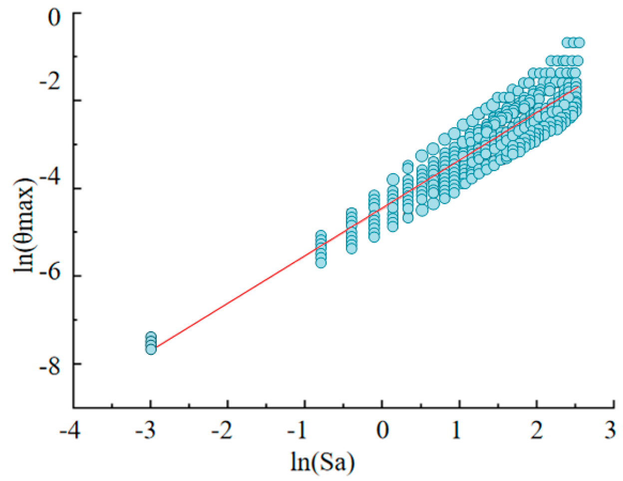
Assuming that both IM and DM follow an exponential distribution, and taking the logarithm of each of these two indicators, the relationship between IM and DM is as shown in Equation (3).
ln D M = A + B ln I M
A coordinate system was established with the natural logarithm of Sa(T1,5%) as the variable and the natural logarithm of θmax as the dependent variable, and scatter plots were drawn. Statistical regression was performed on the IDA analysis data, and the regression curves under different intensities of seismic effects were derived by linear fitting, as shown in Figure 11. The correlation equation is as follows.
ln θ m a x = 4.4750 + 1.0723 ln S a T 1 , 5 %

3.2.2. The Fragility Curves Parameterized by Sa

The performance levels of different structures are classified according to different criteria. Men et al. [34] refined the performance assessment criteria for hybrid frame structures by classifying them into five levels and disclosing the maximum interstory displacement angular limits of the structures at each level, which are detailed in Table 5. Determining the maximum interstory displacement angular limits [35] corresponding to the five types of limit states specified above, the exceedance probability of the structure can be estimated under various seismic forces.
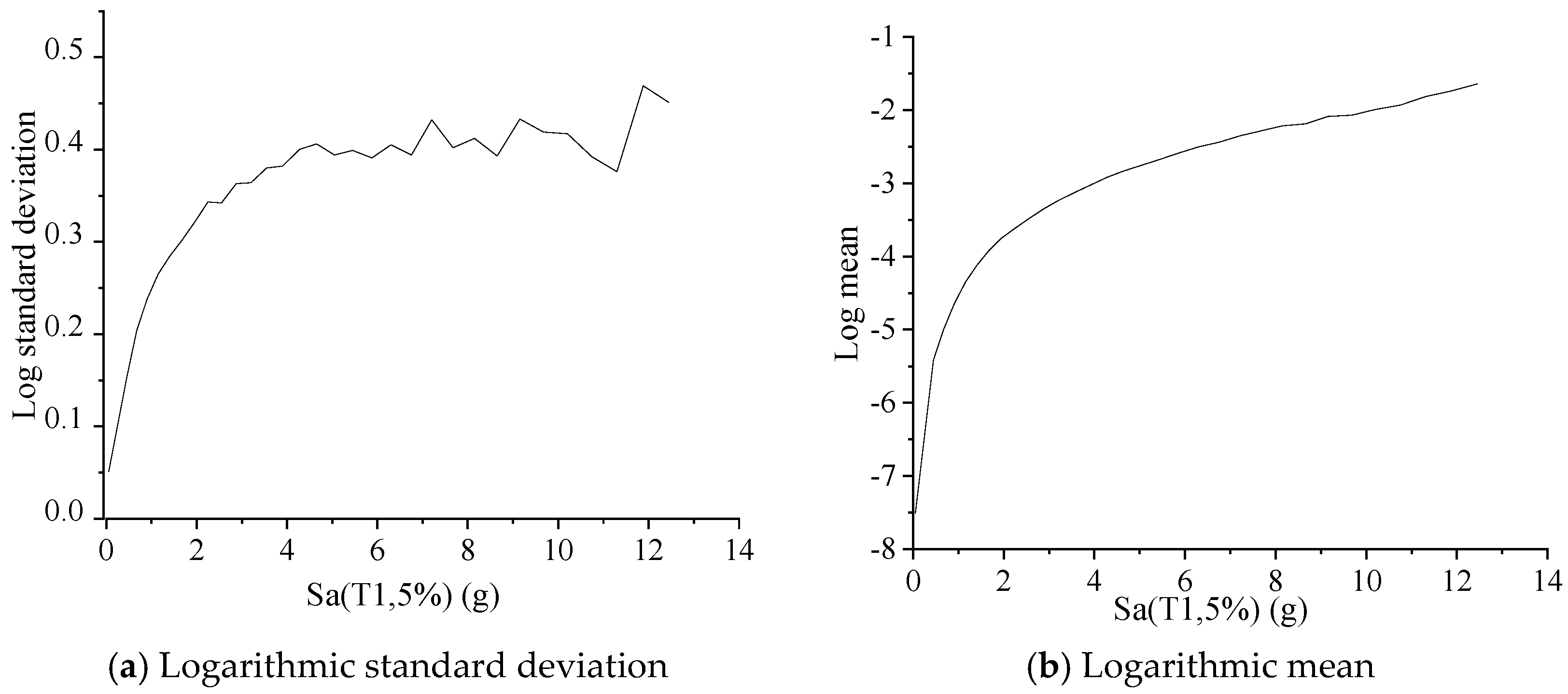
Find the logarithmic mean μ ln D M I M = x and the logarithmic standard deviation σ ln D M I M = x of the maximum interstory displacement angle of the structure for different values of Sa(T1,5%) and substitute these two values into Equation (5) of the semi-probabilistic method. Equation (5) is as follows.
P D M d m i I M = x = 1 P D M < d m i I M = x = 1 Φ ln d m i μ ln D M I M = x σ ln D M I M = x
Take the normal operation limit state LS1 as an example, take the maximum interlayer displacement angular limit as 1/400, when Sa(T1,5%) = 0.05, the logarithmic mean is −7.5109, the logarithmic standard deviation is 0.0512, and substitute them into the above Equation (5) to get:
P θ max 1 / 400 S a T 1 , 5 % = 0.05 = 1 Φ ln 1 / 400 7.5109 0.0512 = 0 %
Taking the maximum interstory displacement angle limit LS1 as an example, the probability that the maximum interstory displacement angle θmax of the structure exceeds the limit LS1 at different Sa(T1,5%) ground motion intensity levels is calculated after amplitude modulation. The results with representative characteristics are selected, as shown in Figure 12. The exceedance probability is 100% but it is 0% when Sa(T1,5%) takes 0.05 g.
By calculation, the values of exceedance probability corresponding to different Sa(T1,5%) for five types of limit states are shown in Figure 13. As can be seen in Figure 13, the slope decreases as the structure changes from LS1 to LS5, indicating that the rate of increase in the exceedance probability of the various performance states of the structure varies as the ground motion increases. When the structure is in an LS1 state, the slope of the curve is larger, indicating that with the increase in IM, the structure easily exceeds the maximum interstory displacement angular limit value of 1/400 at LS1. When the structure is in LS2, LS3, LS4, and LS5 states, the intensity of ground motion becomes larger and larger. And the slope of the curve tends to be flattened, indicating that the structure gradually enters the elastic–plastic state from the elastic state.
From the normal operation state to the preventing collapse state, the interlayer displacement angle limit of the structure becomes larger and larger, and the exceedance probability in the fragility curve gradually decreases at the same ground motion intensity. It can be seen that the seismic performance of this prefabricated hybrid structure is not outstanding in the elastic state, but after transferring to the elastic–plastic state, the steel beams and concrete column–column joints have stronger energy dissipation capacity and better ductility, reflecting good seismic performance.

4. Influencing Factors of Seismic Fragility of Structure

4.1. Concrete Strength

In accordance with the current Chinese code (GB 50011-2016) [27], three frame structure models with column concrete strengths of C30, C40, and C50 were designed, corresponding to Model I-c, Model II-c, and Model III-c, respectively. Model II-c is the original model used for IDA analysis. Except for the column concrete strength, the span, steel beam strength, and other material properties of Model I-c and Model III are consistent with Model II-c.
According to the Chinese code (GB 50010-2010) [36], when conducting elastic–plastic time–history analysis on the structure, the average value of the material strength should be taken, and the specific value can be obtained according to Equation (7). The strength and elasticity modulus of different concretes for each model are shown in Table 6.
f m = f k 1 1.645 δ
IDA analysis based on Sa was performed for Model I-c and Model III-c, respectively. The IDA curves, quantile curves, and conditional logarithmic standard deviations are shown in Figure 14, Figure 15 and Figure 16.
IDA analysis based on PGA was performed for Model I-c and Model III-c, respectively. The IDA curves, quantile curves, and conditional logarithmic standard deviations are shown in Figure 17, Figure 18 and Figure 19.
By comparing Figure 15 and Figure 18, it can be observed that the spread of quantile curves using Sa as the parameter is approximately 5 g, while that using PGA as the parameter is about 5.5 g. Therefore, the quantile curves with Sa as the parameter are more compact than those with PGA as the parameter. Through comparison of Figure 16 and Figure 19, it can be found that the conditional logarithmic standard deviations based on Sa are generally lower than those based on PGA (the values generally differ by 0.1). Consequently, Sa was selected as the parameter for the fragility analysis of the three models.
The data from the IDA analysis were summarized, then taking the natural logarithm of Sa(T1,5%) as the variable and the natural logarithm of θmax as the dependent variable, we constructed a coordinate system, which resulted in a scatterplot. The plots after linear fitting are shown in Figure 20. The equations ln S a T 1 , 5 % ln θ m a x ) of the regression curves for the different models are obtained as shown in Equations (8) and (9).
The relationship equation for the Model I-c regression curve for concrete strength of C30 is Equation (8). And the relationship equation for the Model I-c regression curve for concrete strength of C50 is Equation (9).
ln θ m a x ) = 4.5089 + 1.0776 ln S a T 1 , 5 %
ln θ m a x = 4.4829 + 1.0769 ln S a T 1 , 5 %
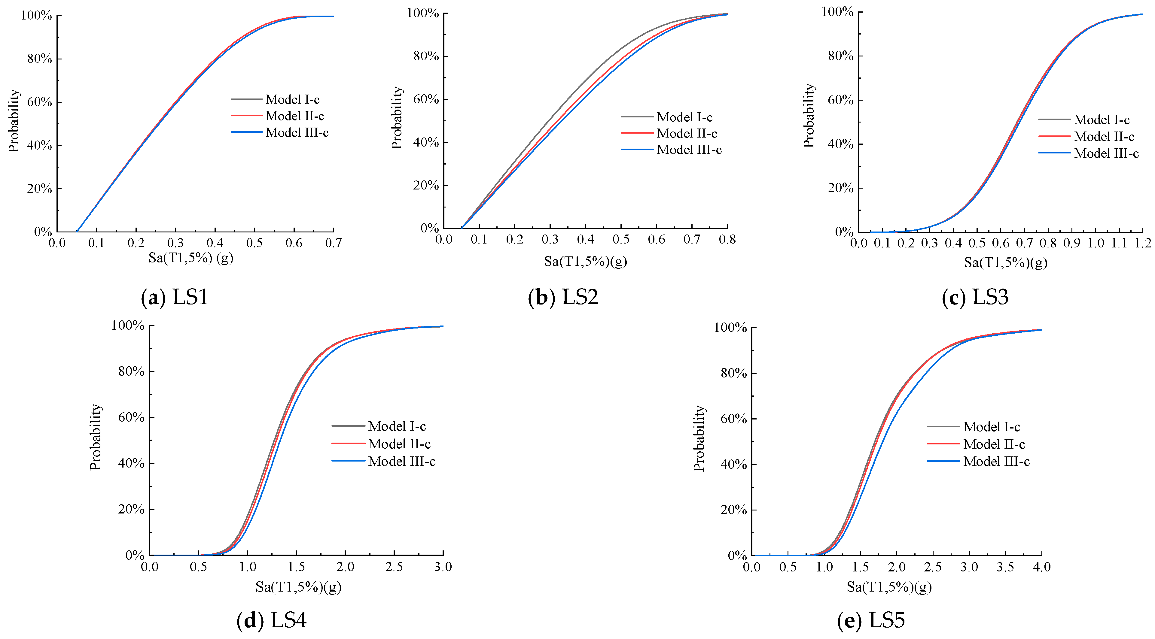
By applying Equation (5) of the semi-probabilistic method, the seismic fragility curves with Sa(T1,5%) as the horizontal axis and the exceedance probability as the vertical axis are obtained as shown in Figure 21.
The fragility curves of the three models at different limit states are plotted separately, as shown in Figure 22. It can be seen that the fragility curves of the three models with different strength grades concrete almost overlap in the LS1 limit state. In the LS2, LS3, LS4, and LS5 limit states, under the different concrete strength grades, it exhibits a consistent trend: Model I-c > Model II-c > Model III-c. The model with higher concrete strength exhibits a lower exceedance probability under the same ground motion intensity. It shows that when the structure is in the elastic stage, the concrete strength does not have much effect on its fragility. With the increase in the ground motion intensity, the structure enters the plastic stage. The RCS hybrid structure has good lateral stiffness, and the increase in the concrete strength plays a role in reducing the exceedance probability.
However, with the increase in concrete strength, the structure’s brittleness increases. Because the RCS structure itself is a steel beam–concrete hybrid structure, the change in concrete strength grade has no effect on the steel beam, resulting in the beam ductility being not greatly improved, while the seismic performance of the structure is not satisfactory.

4.2. Longitudinal Tendon Strength

In accordance with the current Chinese code (GB 50011-2016) [27], three frame structure models with longitudinal reinforcement strengths of HRB335, HRB400, and HRB500 were designed using PKPM software, corresponding to Model I-l, Model II-l, and Model III-l, respectively. Model II-l is the original model used for IDA analysis. In addition to the longitudinal reinforcement strength, the project overview, model span, steel beam strength, and other material properties are consistent with Model II-l.
According to the Chinese code (GB 50010-2010) [36], when conducting elastic–plastic time–history analysis on the structure, the average value of the material strength should be taken, and the specific value can be obtained according to Equation (6). The average value of the longitudinal reinforcement strength and the elasticity modulus for the different models are shown in Table 7.
IDA analysis based on Sa was performed on Model I-l and Model III-l, respectively, and the results were statistically analyzed. The IDA curves, quantile curves, and conditional logarithmic standard deviations are shown in Figure 23, Figure 24 and Figure 25.
IDA analysis based on PGA was performed for Model I-l and Model III-l, respectively, and the results were statistically analyzed. The IDA curves, quantile curves, and conditional logarithmic standard deviations are shown in Figure 26, Figure 27 and Figure 28.
By comparing Figure 24 and Figure 27, it can be observed that the spread of quantile curves using Sa as the parameter is approximately 4.5 g, while that using PGA as the parameter is about 5.0 g. Therefore, the quantile curves with Sa as the parameter are more compact than those with PGA as the parameter. Through comparison of Figure 25 and Figure 28, it can be found that the conditional logarithmic standard deviations based on Sa are generally lower than those based on PGA (the values generally differ by 0.1). Consequently, Sa was selected as the parameter for the fragility analysis of the three models.
The scatterplots obtained by the same above method after linear fitting are shown in Figure 29, and the equations of ln S a T 1 , 5 % ln θ m a x regression curves under different seismic intensity are obtained as follows.
The equation for the Model I-l regression curve for longitudinal reinforcement strength of HRB335 is shown in Equation (10). The equation for the Model III-l for longitudinal reinforcement strength of HRB500 is given by Equation (11).
ln θ m a x ) = 4.4606 + 1.0726 ln S a T 1 , 5 %
ln θ m a x ) = 4.5386 + 1.0827 ln S a T 1 , 5 %
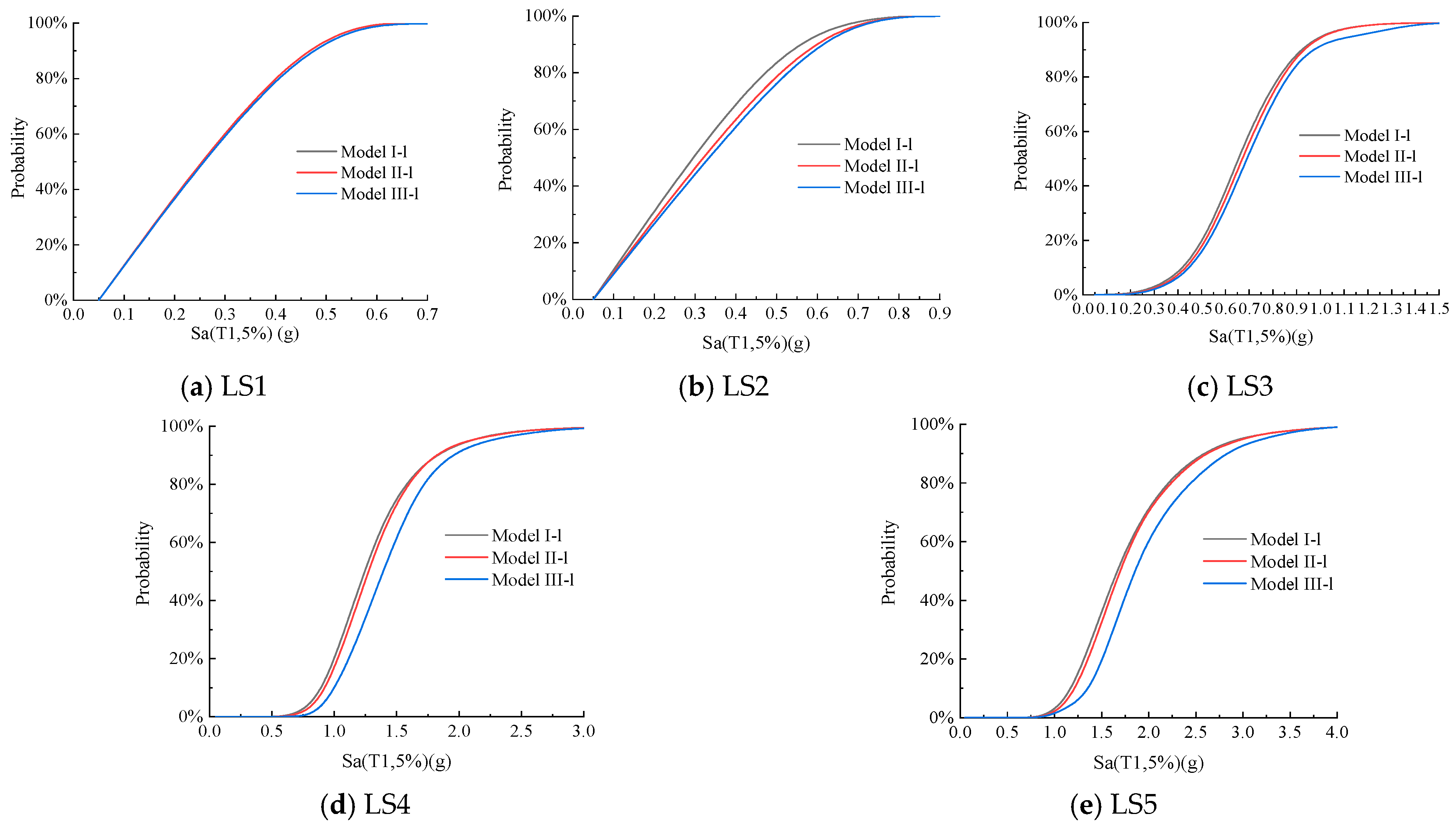
By Equation (5) of the semi-probabilistic method, the seismic fragility curves of the structure with Sa(T1,5%) as the horizontal axis and the exceedance probability as the vertical axis are obtained as shown in Figure 30.
The fragility curves of the three models at different limit states are plotted separately, as shown in Figure 31. It can be seen that the fragility curves of the three models with different longitudinal reinforcement strength almost coincide with each other in the limit state of LS1. In the limit states of LS2, LS3, LS4, and LS5, the longitudinal reinforcement strength of the three models follows the relationship Model I-l > Model II-l > Model III-l. It can be observed that under identical ground motion intensity, models with higher longitudinal reinforcement strength exhibit lower exceedance probabilities. It shows that when the structure is in the elastic stage, the longitudinal reinforcement strength grade does not have much effect on its fragility. With the increase in the ground motion intensity, the structure enters into the plastic stage, and the RCS hybrid structure has good lateral stiffness, while the longitudinal reinforcement plays a role.

4.3. Axial Compression Ratio

Axial Compression Ratio is defined as the ratio of the design axial force on a column to the product of its gross cross-sectional area and the design compressive strength of concrete. It serves as a critical seismic design parameter to control the ductility of frame columns and prevent brittle failure. Therefore, according to the current Chinese Code for Seismic Design of Buildings (GB 50011) [27], three frame structure models with maximum axial compression ratios of 0.57, 0.38, and 0.32 were designed using PKPM software, corresponding to Model I-a, Model II-a, and Model III-a, respectively. Model II-a is the original model used for IDA analysis. In addition to the different axial compression ratios, the project overview, model span, steel beam strength, and other material properties are consistent with Model II-a, and the model design parameters of the different models are shown in Table 8. By the same above method, IDA analysis was performed and the results of IDA curves, quantile curves, and conditional logarithmic standard deviations based on Sa are shown in Figure 32, Figure 33 and Figure 34. The results of PGA are shown in Figure 35, Figure 36 and Figure 37.
By comparing Figure 33 and Figure 36, it can be observed that the spread of quantile curves using Sa as the parameter is approximately 5 g, while that using PGA as the parameter is about 5.5 g. Therefore, the quantile curves with Sa as the parameter are more compact than those with PGA as the parameter. Through comparison of Figure 34 and Figure 37, it can be found that the conditional logarithmic standard deviations based on Sa are generally lower than those based on PGA (the values generally differ by 0.1). Consequently, Sa was selected as the parameter for the fragility analysis of the three models.
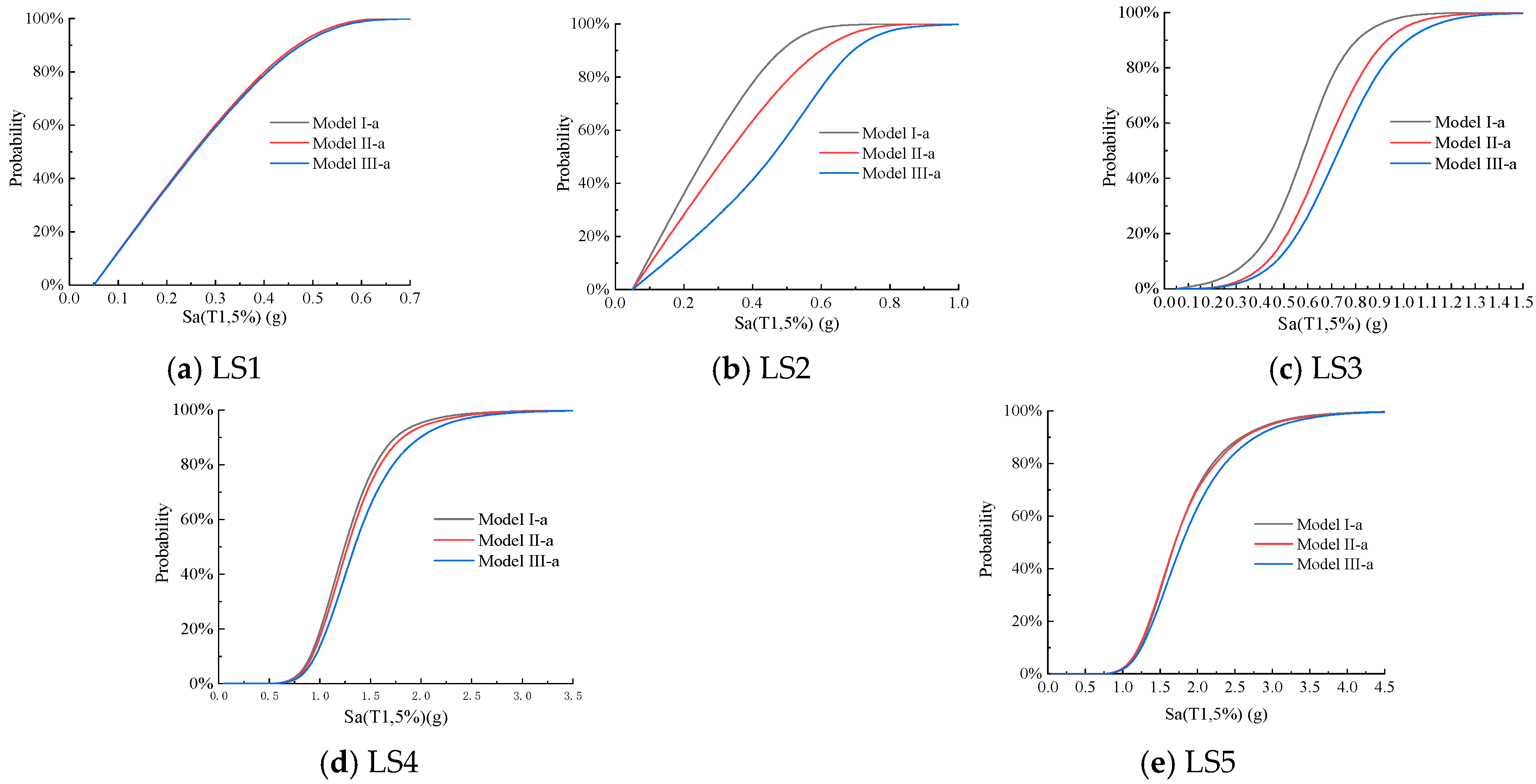
Scatter plots were developed by summarizing the IDA analyze data, and the scatter diagrams after linear fitting are shown in Figure 38, while the relational equations of ln ( S a T 1 , 5 % ) ln θ m a x regression curves are shown in Equations (12) and (13), which are for a maximum axial compression ratio of 0.32 and 0.57, respectively. The seismic fragility curves of the structure with Sa(T1,5%) are shown in Figure 39. The seismic fragility curves of the three models at different limit states are plotted in Figure 40.
ln θ m a x ) = 4.4273 + 1.0403 ln S a T 1 , 5 %
ln θ m a x ) = 4.5386 + 1.0827 ln S a T 1 , 5 %
It can be seen that the fragility curves of three models with different axial compression ratios come under five limit states. Through comparison of Model I-a, Model II-a, and Model III-a, it can be observed that when subjected to the same Sa level, the exceedance probability follows the order of Model I-a > Model II-a > Model III-a. Meanwhile, the axial compression ratios of these three models satisfy the relationship of Model I-a > Model II-a > Model III-a. This indicates that under identical ground motion intensity levels, models with smaller axial compression ratios exhibit lower exceedance probability.
This shows that when the structure is in the elastic stage, the axial compression ratio has little effect on its fragility. With the increase in the ground motion intensity, the structure enters into the plastic stage and the RCS hybrid structure has good lateral stiffness. At the same time, the column cross-sectional area increases, and the axial compression ratio decreases, which results in an increase in structural stiffness, and an increase in the resistance capacity to lateral deformation. With the reduction in the column axial compression ratio, it is favorable for the structure to form the yield mechanism of “strong column and weak beam”. This is the case even if under the action of an earthquake, the structure is first damaged at the end of the beam, and the plastic hinge appears at the end of the beam first. So, the reasonable design of the axial compression ratio should be emphasized.

5. Conclusions

The seismic fragility of prefabricated RCS hybrid frame structures is investigated by the IDA method and the main conclusions are as follows:
(1) From comparison of the two ground motion intensity indicators, Sa(T1,5%) and PGA, it is revealed that Sa(T1,5%) is a more appropriate parameter to analyze the fragility of prefabricated RCS hybrid frame structures.
(2) The seismic performance of this prefabricated RCS hybrid frame is not outstanding in the elastic state. In the elastic–plastic state, the steel beams and concrete column–column joints have stronger energy dissipation capacity and better ductility, reflecting good seismic performance.
(3) Increasing the concrete strength enhances the bearing capacity, but the structure’s brittleness increases and does not improve the ductility of the structure. Longitudinal reinforcement strength in the plastic phase improves the lateral stiffness. The increase in the column cross-sectional area can reduce the axial compression ratio, improve the structural stiffness, and promote the formation of the “strong columns and weak beams” yield mechanism. It provides reference for the design of prefabricated RCS hybrid frame structures.

Author Contributions

Y.W.: conceptualization, supervision. G.S.: investigation, methodology, writing—original draft preparation. X.W.: methodology, writing—review and editing. X.Z.: investigation, methodology. C.M.: validation, supervision. All authors have read and agreed to the published version of the manuscript.

Funding

This work was supported by Scientific Research Project of Tianjin Education Commission (2019ZD17).

Data Availability Statement

The original contributions presented in the study are included in the article, further inquiries can be directed to the corresponding author.

Conflicts of Interest

The authors declare that there are no conflicts of interest.

References

  1. Jian, Z. Study on Vulnerability Analysis and Seismic Risk of Reinforced Concrete Structures; Xi’an University of Architecture and Technology: Xi’an, China, 2010. [Google Scholar]
  2. Vamvatsikos, D.; Cornell, C.A. Incremental dynamic analysis. Earthq. Eng. Struct. Dyn. 2002, 31, 491–514. [Google Scholar] [CrossRef]
  3. Beitz, W.; Pahl, G.; Grote, K. Engineering design: A systematic approach. Mrs Bulletin. 1996, 71, 30. [Google Scholar]
  4. Fazli, H. Optimal performance-based seismic design of composite building frames with RC columns and steel beams. Int. J. Optim. Civ. Eng. 2019, 9, 611–628. [Google Scholar]
  5. Fan, D.; Jinjie, M.; Zhang, Z.; Wenye, T.; Yunlong, L. Seismic Performance and Replaceability Analysis of RCS Hybrid Frame with Energy Dissipation Beams; SSRN: Rochester, NY, USA; p. 5114963.
  6. Si, Q.; Pan, Z.; Zhu, Y.; Ying, H. Seismic design method based on limit state for prefabricated RCS frames. Structures 2024, 59, 105747. [Google Scholar] [CrossRef]
  7. Murari, K.; Kumar, P.C.A.; Shiradhonkar, S. Analytical investigations of seismic performance of different joint details for composite RCS frames. CE/papers 2023, 6, 46–52. [Google Scholar] [CrossRef]
  8. Dai, H.; Wang, B. Seismic Analysis of steel solid web girder-RC tubular column hybrid structure. Appl. Sci. 2018, 8, 2095. [Google Scholar] [CrossRef]
  9. Ghezeljeh, J.; Mirghaderi, S.R.; Kavei, S. Comparison of the seismic performance of Reinforced Concrete-Steel (RCS) frames with steel and reinforced concrete moment frames in low, mid, and high-rise structures. Steel Compos. Struct. 2024, 50, 249–263. [Google Scholar]
  10. Men, J.J.; Huo, W.W.; Lan, T.; Lei, M.K.; Shi, Q.X. Mechanical behavior and seismic design method of RCS hybrid frame structure with replaceable components. China Civ. Eng. J. 2020, 53, 42–52. [Google Scholar]
  11. Pan, Z.; Si, Q.; Zhu, Y.; Ying, H.; Wang, X.; Du, D. Seismic performance of prefabricated semi-rigid RCS structures. Structures 2022, 43, 1369–1379. [Google Scholar] [CrossRef]
  12. Cai, J.; Li, W. Seismic performance of demountable RCS frame structures. Earthq. Eng. Eng. Vib. 2025, 45, 205–216. (In Chinese) [Google Scholar]
  13. Bertero, V.V. Strength and deformation capacities of buildings under extreme environments. Struct. Eng. Struct. Mech. 1977, 53, 29–79. [Google Scholar]
  14. Vamvatsikos, D.; Cornell, C.A. Applied incremental dynamic analysis. Earthq. Spectra 2004, 20, 523–553. [Google Scholar] [CrossRef]
  15. Dolsek, M. Incremental dynamic analysis with consideration of modeling uncertainties. Earthq. Eng. Struct. Dyn. 2009, 38, 805–825. [Google Scholar] [CrossRef]
  16. Cheng, Y.; Dong, Y.R.; Bai, G.L.; Wang, Y.Y. IDA-based seismic fragility of high-rise frame-core tube structure subjected to multi-dimensional long-period ground motions. J. Build. Eng. 2021, 43, 102917. [Google Scholar] [CrossRef]
  17. Jouneghani, H.G.; Haghollahi, A. Assessing the seismic behavior of steel moment frames equipped by elliptical brace through incremental dynamic analysis (IDA). Earthq. Eng. Eng. Vib. 2020, 19, 435–449. [Google Scholar] [CrossRef]
  18. Fanaie, N.; Ezzatshoar, S. Studying the seismic behavior of gate braced frames by incremental dynamic analysis (IDA). J. Constr. Steel Res. 2014, 99, 111–120. [Google Scholar] [CrossRef]
  19. Wu, C.; Pan, Z.; Jin, C.; Meng, S. Evaluation of deformation-based seismic performance of RECC frames based on IDA method. Eng. Struct. 2020, 211, 110499. [Google Scholar] [CrossRef]
  20. Ren, H.; Tian, Q.H.; Zhang, W.C.; Zhou, C.F.; Shao, D. Seismic fragility analysis of reinforced concrete frame structures based on IDA method. Build. Struct. 2019, 49, 350–355. (In Chinese) [Google Scholar]
  21. Li, G.; Dong, Z.Q.; Li, H.N.; Yang, Y.B. Seismic collapse analysis of concentrically-braced frames by the IDA method. Adv. Steel Constr. 2017, 13, 273–292. [Google Scholar]
  22. Xu, W.; Zhao, Y.; Yang, W.; Yu, D.; Zhao, Y. Seismic fragility analysis of RC frame structures based on IDA analysis and machine learning. Structures 2024, 65, 106774. [Google Scholar] [CrossRef]
  23. Liu, X.; Xu, C. IDA-Based Seismic fragility analysis of a concrete-filled square tubular frame. Buildings 2024, 14, 2686. [Google Scholar] [CrossRef]
  24. Qiu, Y.C.; Zhou, J.Z.; Yang, G.X. Ductility analysis of RC frames based on IDA. J. Hefei Univ. Technol. (Nat. Sci. Ed.) 2015, 38, 377–382. (In Chinese) [Google Scholar]
  25. Li, J.; Chen, P.; Wei, W.; Li, Q.N. Seismic behavior research of steel plate hoop-bolt prefabricated column confined by high-strength composite spiral stirrups. Ind. Constr. 2014, 44, 7–10. (In Chinese) [Google Scholar]
  26. Huang, S.M.; Wang, Y.Y.; Dai, G.Y.; Fu, S.C.; Luo, K.H.; Li, X.J.; Ke, C.H.; Yu, Y.Q.; Lou, Y.; Xue, H.L. Seismic Design Code for Buildings (GB 50011-2016). China Build. Ind. Press 2016, 8. [Google Scholar]
  27. Mander, J.B. Theoretical Stress-Strain Model or for Confined Concrete. J. Struct. Devision 1988, 114, 1804–1826. [Google Scholar] [CrossRef]
  28. Azarbakht, A. Minimum magnitude boundaries in probabilistic seismic hazard analysis: An insight from structural engineering. Bull. Earthq. Eng. 2024, 22, 5299–5320. [Google Scholar] [CrossRef]
  29. Applied Technology Council; National Earthquake Hazards Reduction Program (US). Seismic Performance Assessment of Buildings; Federal Emergency Management Agency: Washington, DC, USA, 2012.
  30. Iervolino, I.; Cornell, C.A. Record Selection for Nonlinear Seismic Analysis of Structures. Earthq. Spectra 2005, 21, 685–713. [Google Scholar] [CrossRef]
  31. Baker, J.W. Efficient analytical fragility function fitting using dynamic structural analysis. Earthq. Spectra 2015, 31, 579–599. [Google Scholar] [CrossRef]
  32. Kazemi, F.; Asgarkhani, N.; Jankowski, R. Machine learning-based seismic fragility and seismic vulnerability assessment of reinforced concrete structures. Soil Dyn. Earthq. Eng. 2023, 166, 107761. [Google Scholar] [CrossRef]
  33. Wang, L. Effectiveness of New Ground Motion Intensity Measures Based on IDA and Seismic Fragility Analysis of Structures; Lanzhou University of Technology: Lanzhou, China, 2020. [Google Scholar]
  34. Men, J.J.; Zhou, T.T.; Zhang, Y.R.; Shi, Q.X. Performance-based seismic design method and quantitative index for reinforced concrete column-steel beam composite frame structures. J. Build. Struct. 2015, 36, 28–34. (In Chinese) [Google Scholar]
  35. FEMA-356; Prestandard and Commentary for the Seismic Rehabilitation of Buildings. Federal Emergency Management Agency: Washington, DC, USA, 2000.
  36. Zhao, K.D.; Liu, L.X.; Qiu, H.X.; Huang, X.K.; Zhu, A.P.; Wang, X.F.; Fu, J.P.; Ke, C.H.; Zhang, F.X.; Zuo, J. Code for design of concrete structures (GB 50010-2010). Constr. Sci. Technol. 2015, 3. [Google Scholar]
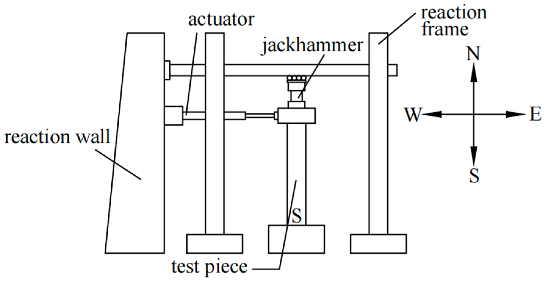
Figure 1. Test loading device.
Buildings 15 03207 g001
Figure 2. Lateral loading protocol.
Buildings 15 03207 g002
Figure 3. Column–column joint model.
Buildings 15 03207 g003
Figure 4. Comparison of hysteresis curves.
Buildings 15 03207 g004
Figure 5. Structural details.
Buildings 15 03207 g005
Figure 6. Kern County wave.
Buildings 15 03207 g006
Figure 7. Kern County wave IDA curve.
Buildings 15 03207 g007
Figure 8. IDA curves for 12 seismic waves.
Buildings 15 03207 g008
Figure 9. Quantile curve.
Buildings 15 03207 g009
Figure 10. Conditional logarithmic standard deviation.
Buildings 15 03207 g010
Figure 11. Seismic probability demand model curve.
Buildings 15 03207 g011
Figure 12. Values of each parameter corresponding to different Sa(T1,5%).
Buildings 15 03207 g012
Figure 13. Values of exceedance probability corresponding to different Sa(T1,5%) for five types of limit states.
Buildings 15 03207 g013
Figure 14. IDA curves based on Sa for different concrete strength.
Buildings 15 03207 g014
Figure 15. Quantile curves based on Sa for different concrete strength.
Buildings 15 03207 g015
Figure 16. Conditional logarithmic standard deviations based on Sa for different concrete strength.
Buildings 15 03207 g016
Figure 17. PGA-based IDA curves.
Buildings 15 03207 g017
Figure 18. PGA-based quantile curves.
Buildings 15 03207 g018
Figure 19. Conditional logarithmic standard deviation based on PGA for different concrete strength.
Buildings 15 03207 g019
Figure 20. Seismic probability demand model curve based on Sa for different concrete strength.
Buildings 15 03207 g020
Figure 21. Seismic fragility curve based on Sa for different concrete strength.
Buildings 15 03207 g021
Figure 22. Fragility curves of the structure at different limit states for different concrete strength.
Buildings 15 03207 g022
Figure 23. IDA curves based on Sa for different longitudinal tendon strength.
Buildings 15 03207 g023
Figure 24. Quantile curves based on Sa for different longitudinal tendon strength.
Buildings 15 03207 g024
Figure 25. Conditional logarithmic standard deviations based on Sa for different longitudinal tendon strength.
Buildings 15 03207 g025
Figure 26. IDA curves based on PGA.
Buildings 15 03207 g026
Figure 27. Quantile curves based on PGA for different longitudinal tendon strength.
Buildings 15 03207 g027
Figure 28. Conditional logarithmic standard deviations based on PGA for different longitudinal tendon strength.
Buildings 15 03207 g028
Figure 29. Seismic probability demand model curve based on Sa for different longitudinal tendon strength.
Buildings 15 03207 g029
Figure 30. Seismic fragility curve of the structure based on Sa for different longitudinal tendon strength.
Buildings 15 03207 g030
Figure 31. Fragility curves of the structure at different limit states for different longitudinal tendon strength.
Buildings 15 03207 g031
Figure 32. IDA curves based on Sa for different axial compression ratio.
Buildings 15 03207 g032
Figure 33. Quantile curves based on Sa for different axial compression ratio.
Buildings 15 03207 g033
Figure 34. Conditional logarithmic standard deviation based on Sa for different axial compression ratio.
Buildings 15 03207 g034
Figure 35. IDA curves based on PGA for different axial compression ratio.
Buildings 15 03207 g035
Figure 36. Quantile curves based on PGA for different axial compression ratio.
Buildings 15 03207 g036
Figure 37. Conditional logarithmic standard deviation based on PGA for different axial compression ratio.
Buildings 15 03207 g037
Figure 38. Seismic probability demand model curves based on Sa for different axial compression ratio.
Buildings 15 03207 g038
Figure 39. Seismic fragility curves for structures based on Sa.
Buildings 15 03207 g039
Figure 40. Fragility curves of the structure at different limit states for different axial compression ratio.
Buildings 15 03207 g040
Table 1. Specimen test design parameters.
Specimen NumberRatio of Axial Compression Stress to StrengthAxial Pressure (kN)Shear-span RatioMaximum Horizontal Load (kN)Loading Method
PRCC-010.2857.64.5249.3low-cyclic recurrence
Table 2. The difference in ultimate load.
Cycle NumberDisplacement (mm)Test Value (kN)Value of Simulation (kN)Difference (%)
114.57223.15208.130.15
222.83234.57220.430.14
335.18210.13198.790.11
447.96203.35186.550.16
559.17187.65175.340.12
675.62177.48164.210.13
Table 3. Structural vibration model period.
Modal OrderPeriod (s)Modal Shapes
10.7767Y-direction translational motion
20.2190X-direction translational motion
30.1840Torsion
Table 4. Results under Kern County wave.
Serial NumberStep Size Calculation MethodSa(T1,5%)/gAmplitude Modulation Index λ Interlayer   Displacement   Angle   θ max
1 0.050.26800.0006
20.05 + 0.40.452.41210.0039
30.45 + 0.4 + 0.050.904.82420.0095
40.90 + 0.4 + 2 × 0.051.407.50430.0179
51.40 + 0.4 + 3 × 0.051.9510.45240.0278
61.95 + 0.4 + 4 × 0.052.5513.66850.0357
72.55 + 0.4 + 5 × 0.053.2017.15270.0455
83.20 + 0.4 + 6 × 0.053.9020.90480.0526
93.90 + 0.4 + 7 × 0.054.6524.92500.0625
104.65 + 0.4 + 8 × 0.055.4529.21310.0714
115.45 + 0.4 + 9 × 0.056.3033.76930.0833
126.30 + 0.4 + 10 × 0.057.2038.59350.0909
137.20 + 0.4 + 11 × 0.058.1543.68570.1111
14(0.45 + 0.90)/20.6753.61810.0064
15(0.90 + 1.40)/21.156.16420.0137
16(1.40 + 1.95)/21.6758.97830.0227
17(1.95 + 2.55)/22.2512.06050.0313
18(2.55 + 3.20)/22.87515.41060.0400
19(3.20 + 3.90)/23.5519.02870.0500
20(3.90 + 4.65)/24.27522.91490.0588
21(4.65 + 5.45)/25.0527.06900.0667
22(5.45 + 6.30)/25.87531.49120.0769
23(6.30 + 7.20)/26.7536.18140.0909
24(7.20 + 8.15)/27.67541.13960.10000
Table 5. Limit value of interstory displacement angle for RCS hybrid frame.
Performance LevelNormal Operation
(LS1)
Temporary Use (LS2)Use After Repair
(LS3)
Life Safety
(LS4)
Preventing Collapse
(LS5)
Limit value of inter-story displacement angle1/4001/2501/1501/701/50
Table 6. The strength and elasticity modulus of different concretes for each model.
Model NumberModel I-cModel II-cModel III-c
Concrete strength classC30C40C50
Average concrete strength (MPa)33.0542.5152.33
Modulus of elasticity (MPa)3.30 × 1043.51 × 1043.67 × 104
Table 7. Mean values of different longitudinal reinforcement strength and elasticity modulus.
Model NumberModel I-lModel II-lModel III-l
Strength grade of longitudinal reinforcementHRB335HRB400HRB500
Average strength of longitudinal reinforcement (MPa)378.60452.05565.07
Table 8. Cross-sectional dimensions of beams and columns and maximal axial compression ratio for each model.
Model NumberModel I-aModel II-aModel III-a
Beam section dimensionH400 × 146 × 14.5 × 14.5
Column section dimension500 × 500600 × 600700 × 700
Maximal axial compression ratio0.570.380.32
Disclaimer/Publisher’s Note: The statements, opinions and data contained in all publications are solely those of the individual author(s) and contributor(s) and not of MDPI and/or the editor(s). MDPI and/or the editor(s) disclaim responsibility for any injury to people or property resulting from any ideas, methods, instructions or products referred to in the content.