Abstract
This study proposes an energy-based framework for evaluating the seismic ductility of reinforced concrete (RC) structures using restoring force hysteresis curves. A custom-developed tool, the Damage Energy Calculation Program (DECP), is introduced to compute cumulative hysteretic energy and corresponding damage indices from experimental data. Seven methods for identifying yield displacement and yield load are examined, encompassing stiffness-based and energy-based techniques, including the conditional yield method, secant stiffness method, and double energy equivalence method. These methods are applied to a series of experimental restoring force curves (SP01 to SP10). Among them, the double energy equivalence method demonstrates the highest accuracy in capturing the yield state. Additionally, a novel ductility index based on the maximum energy envelope is proposed. Comparative analysis shows that this new index exhibits trends consistent with the double energy equivalence approach, highlighting its potential as a reliable alternative. The DECP tool significantly improves the consistency and efficiency of ductility assessment and offers practical support for energy-based damage evaluation in structural performance analysis.
1. Introduction
Due to the inherent uncertainty in seismic ground motions, structures must be designed to ensure reliable energy dissipation and adequate ductility. In ductile moment-resisting frames, the strong-column–weak-beam design approach is applied to promote plastic hinge development in beams rather than columns, thereby maintaining the vertical load-bearing capacity during seismic events [1]. Since structural columns are allowed to enter the elastoplastic damage stage [2], it is imperative to consider the strengthening of the bearing capacity and elastoplastic deformation capacity of the structure in the elastoplastic stage. The displacement-based elastoplastic deformation capacity is usually demonstrated by the ductility index , which is of great significance [3] to determine whether a structure can survive in the earthquake. Previous studies have indicated that the shear-span ratio , the reinforced concrete strength grade , the axial compression ratio , the longitudinal reinforcement ratio (the ratio between height and span (shear-span ratio, λ), and the ratio of applied axial load to column capacity (axial load ratio) and the stirrup ratio are the main influencing factors [4,5] of ultimate bearing ductility capacity. For instance, energy dissipation in steel-reinforced concrete (SRC) columns increases with higher axial load ratios and shear-span ratios [6], while RC walls with low shear-span ratios exhibit greater hysteretic energy capacity [7]. Moreover, simplified residual displacement methods establish a correlation between static/dynamic displacement and energy dissipation in RC systems. [8]. The yield point of the test specimen with a low reinforcement ratio and an obvious yield point can be determined by the reinforcement - measurement and - curve. When the reinforcement member with a high reinforcement ratio yields, it is difficult to determine the yield point by the - curve. If the yield point is not unanimously defined, structural behaviors cannot be consistently described [9]. The literature indicates that yield displacement derived from nonlinear dynamic analysis exhibits greater stability across varying load histories [10]. Ma et al. [11] provided foundational experimental data on the hysteretic behavior of reinforced concrete (RC) beams subjected to both cyclic and monotonic loading. Additionally, reliability-based ductility reduction surfaces have been developed to quantify ductility demand using energy-based seismic intensity measures [12]. Bruneau and Wang [13] demonstrated that, under rectangular excitation, hysteretic energy correlates closely with displacement ductility measures—an observation further supported by Ling et al. [14].
Concurrently, advancements in constitutive modeling and strength theories have highlighted key mechanical challenges and research directions for structural materials [15]. For example, Bigoni and Piccolroaz’s yield surface formulation effectively captures damage-induced transitions from quasi-brittle to ductile behavior in concrete [16]. Standardization efforts by Davidson et al. [17] established consistent procedures for determining yield displacement and cyclic loading protocols in structural ductility evaluations. More recently, machine learning approaches have been applied to predict seismic energy dissipation in RC shear walls, identifying critical parameters influencing hysteretic energy behavior [18].
Overall, seismic ductility assessment of RC and steel-reinforced concrete (SRC) columns increasingly favors energy-based hysteretic methods over traditional force- or displacement-based metrics due to their superior correlation with cumulative damage and post-yield performance. Deng et al. [19] showed that high-ductility fiber-reinforced concrete (HDC) columns dissipate significantly more hysteretic energy post-cracking, indicating enhanced seismic resilience compared to conventional RC columns. Similarly, studies on freeze–thaw-degraded RC columns revealed marked reductions in cumulative hysteretic energy and damping capacity, underscoring the value of energy metrics for durability assessment [20]. Post-retrofit testing of RC columns strengthened with carbon fiber sheets demonstrated dramatic increases, up to approximately 800%, in displacement ductility and energy dissipation, especially under shear failure modes [21]. Refs. [20,21] provided foundational experimental data and highlighted limitations in traditional ductility measures, motivating the development of the DECP tool to standardize energy-based analysis. Investigations of recycled concrete-filled steel tube (RCFST) columns confirmed that energy-based yield definitions, established via bi-linear energy equivalence curves, yield stable ductility values (μ > 3) across various parametric changes [22]. These findings extend to bridge column evaluations, where parametric studies have linked geometric aspect ratios directly to displacement ductility under cyclic loading conditions [23]. Hybrid SRC-RC systems with refined seismic detailing exhibited improved hysteretic loop stability and enhanced energy dissipation efficiency [24]. Evaluations of high-strength concrete columns further validated that energy-equivalent yield definitions align closely with peak displacement metrics, reinforcing their applicability in ductility characterization [25,26]. Nevertheless, the literature consistently highlights the lack of consensus on definitions of yield displacement and ultimate displacement, motivating calls for standardized, energy-based thresholding methodologies. Table 1 presents an overview of the literature in this domain.

Table 1.
Literature summarization.
Considering the foregoing discussion, in this paper, seven independent methods for calculating the yield displacement and the yield load in the ultimate bearing ductility index are utilized and analyzed for the test member whose yield load and yield displacement cannot be easily determined. The seven calculation methods and their main algorithm flows are presented. These seven selected methods differ in their theoretical basis; some use geometric or stiffness approximations, while others rely on energy equivalence principles, to identify yield parameters from hysteretic data. Among these, the double energy equivalence method is emphasized due to its consistent convergence with experimental results and its physical basis in closed-loop energy symmetry. Based on the calculation results of the ultimate bearing capacity ductility index of the proposed seven methods, this paper finally adopts the ductility coefficient based on the bi-parametric energy equivalence method as the ductility index to evaluate the ultimate bearing capacity.
Overall, despite extensive research on seismic ductility, there is still no consensus on how to define or determine the yield displacement and force from hysteresis curves, particularly in structures exhibiting nonlinear or degrading behavior. This lack of standardization leads to inconsistent ductility assessments, which can compromise both design and retrofit decisions. To address this issue, this study develops and evaluates seven yield calculation methods using a dedicated analysis tool (DECP), and proposes a novel maximum envelope energy ductility index for improved evaluation of elastoplastic response in RC structures, which defines the novelty of this paper.
2. Methods/Experimental
2.1. Method and Program for Calculating Damage Energy of Restorative Hysteresis Curve
Confronted with a large number of cumulate energy data in a quasi-static test, it is necessary to import each column (where x denotes horizontal displacement under quasi-static cyclic loading) and analyze the determination and selection of each critical state in each data cycle. Due to the complex and cumbersome positive and negative loading calculation of energy and the loop-based calculation of separate and cumulate energy, it is far from enough to use the commercial software YJK(V7.0) or ORIGIN(2025) to calculate the energy. Therefore, the calculation method and program for calculating the cumulate energy of the restoring force based on the quasi-static test shall be developed. In this paper, the calculation principle of the hysteresis loop’s cumulate energy in the restoring force’s constitutive curve and the corresponding damage index method are analyzed in detail. Moreover, according to the proposed cumulate energy calculation method, a MATLAB (2025) program is compiled, which is defined as the Damage Energy Calculation Program (DECP). The hysteretic energy correlates with structural damage and energy dissipation capacity, making it a reliable metric for evaluating seismic performance and degradation
2.1.1. Damage Energy Programming and Process
The standard hysteresis loop analysis method in the DECP program is illustrated by the schematic diagram of the independent standard hysteresis loop ( loop), as can be seen in Figure 1. Figure 1 is a conceptual diagram and illustrates the control points for algorithm implementation, not actual test data. Taking the standard loop curve () as an example, the programming process and algorithm of ten control points ①⑩ are described. In the DECP program, ten control points ①⑩ are identified by programming, and the algorithm for determining the starting and ending positions is specified below: when the program continuously reads five positive values, it means that the restoring force test curve starts to load in the positive direction; otherwise, it means that the restoring force test curve starts to load in the negative direction (that is, the end of unloading in the positive direction).
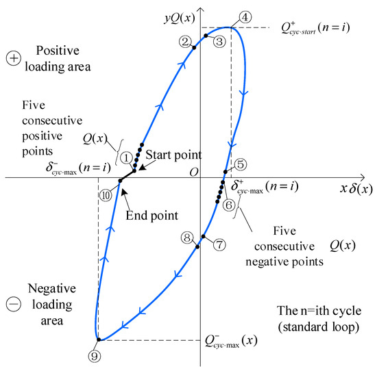
Figure 1.
Schematic diagram of the standard (i-th) restoring force loop. Note: The i-th loop is selected as the reference loop. Its area is calculated and added to the total cumulative area. Based on this and other calculated indicators, the maximum envelope energy area is defined. Five consecutive data points in the positive or negative direction are used to determine loading trends.
2.1.2. Analysis and Calculation of Main Influencing Indicators for the Standard Loop
(1) Calculation of the standard loop’s elastic energy . It is assumed that the standard loop is adopted. In the positive loading area (y > 0), the elastic energy for each cycle can be calculated by the formula . In the negative loading area (y < 0), the elastic energy for each cycle can be calculated by the formula . The sum in the positive and negative directions can be calculated by wherein , as shown in Figure 2.
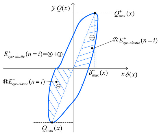
Figure 2.
Schematic of restoring force loop segments under cyclic loading, showing energy dissipation in both directions.
(2) Calculation of the standard loop’s hysteretic energy for each cycle. When y > 0, the hysteretic energy of the loop for each cycle is written into ; when y < 0, the hysteretic energy of the loop for each cycle is written into . Additionally, for a single cycle, + , as shown in Figure 3.
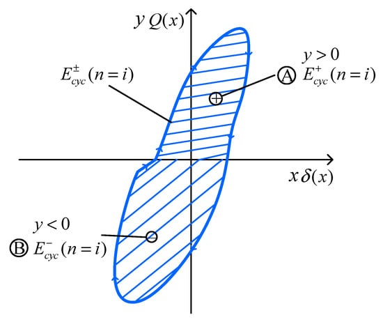
Figure 3.
Schematic diagram of hysteretic energy for each cycle in the standard loop of the restoring force curve.
2.1.3. Calculation of Cumulate Elastic Energy in the Standard Loop of the Restoring Force Curve
- (1)
- Sum of cumulate elastic energy for each cycle:
- (2)
- Sum of cumulate hysteretic energy for each circle:
- (3)
- Specific damping of cumulate hysteretic energy for each circle:
- (4)
- Cumulate elastic energy for each cycle:
- (5)
- Cumulate hysteretic energy for each cycle:
- (6)
- Specific damping of cumulate energy for each cycle:
- (7)
- Final sum of the total elastic energy for each cycle:
- (8)
- Final sum of the total hysteretic energy for each cycle:
- (9)
- Method for calculating damage energy :
- (10)
- Method for calculating damage index :
To sum up, the key influencing indexes of the restoring force curve in the above test are calculated and recorded in the DECP program.
2.1.4. Method and Program for Calculating the Skeleton Curve of the Restoring Force
The skeleton curve, which describes the envelope curve connecting the peak points from each hysteresis loop cycle, used to represent the overall structural stiffness degradation, of the restoring curve is composed of the control points of each restoring force curve for each cycle, namely, and , wherein . Based on the analyses of the restoring force curve test data in the DECP program, the control point indexes of the skeleton curve for each test member are identified and determined, and the data are saved, as shown in Figure 4.
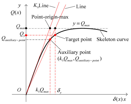
Figure 4.
Schematic diagram of the universal yield moment calculation based on DECP.
2.2. Calculation Method and Analysis of Ultimate Ductility Index Based on DECP
After introducing the calculation method of damage energy in the restoring force curve and the main technical steps, it is known that the DECP program can be used for dealing with all kinds of complicated and diverse hysteretic test curve data, and the main control parameters can be obtained through the program calculation. Meanwhile, the control indexes for the skeleton curve in the restoring force curve can be identified and solved. Next, the ultimate ductility index is calculated and analyzed based on DECP. In this paper, seven calculation methods are adopted for calculating and analyzing the yield displacement and yield load in the ultimate bearing ductility index , and the index is also analyzed and assessed.
These following subsections outline the methodology used to compute ductility indices and damage parameters from hysteresis curves of reinforced concrete members. The primary goal is to evaluate and compare seven widely referenced methods for determining yield displacement and yield force from cyclic test data. The DECP (Damage Energy Calculation Program) was developed in MATLAB (2025) to process and analyze these curves efficiently. The hypotheses guiding this analysis are as follows: (1) energy-based methods offer improved consistency in yield determination for nonlinear cyclic curves, and (2) double energy equivalence provides better convergence with observed behavior. All methods are evaluated on the same dataset for consistency, and their performance is compared through calculated ductility indices.
To improve clarity, detailed programming logic has been provided in Appendix A and MATLAB codes in Supplementary Materials. Here, we focus on summarizing each method’s principle and algorithmic logic with reference to the figures provided.
2.2.1. Method I: Conditional Yield Calculation
This method identifies the yield point based on the first yielding of reinforcement as observed in test data. It is often applied when a distinct yield plateau exists. The yield displacement and force are extracted based on data processing of strain data. This serves as the baseline method for comparison. According to the data collected from the steel bar of the structural member, the yield state of the steel bar is determined as the member yield, which can be obtained by analyzing and processing the test data. The pseudo code designed for this purpose is presented in Appendix A.1. and the corresponding MATLAB code in Supplementary Materials.
2.2.2. Method II: Universal Yield Moment Calculation
The calculation method of the universal yield moment is shown in Figure 5. ① Cross the origin, take as the loading stiffness, and draw a straight line to intersect with the straight line , where the intersection point is point-origin-max. Call and , and extend to intersect with at point-origin-max, whose coordinates are . ② Draw a vertical line through point-origin-max to intersect with the skeleton curve, with the intersection point as an auxiliary point, whose coordinates are , and the slope is = . ③ By connecting the origin and auxiliary point, the slope and intersect at the skeleton curve, namely, ; draw a vertical line through this point to intersect with the skeleton curve and the transverse coordinate finds the corresponding point on the skeleton curve, namely, ).
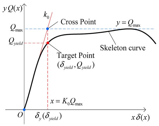
Figure 5.
Schematic diagram of equivalent elastoplastic yield calculation based on DECP.
2.2.3. Method III: Equivalent Elastoplastic Yield Calculation
The yield displacement shall have the same tangent stiffness and strength value as the actual curve. ① Take and find the cross point on the skeleton curve. ② Find the target point of the skeleton curve. ③ The cross-point coordinates are , and the values are recorded. The equivalent elastoplastic yield calculation is shown in Figure 6.
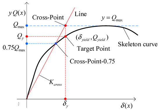
Figure 6.
Schematic diagram of the secant stiffness calculation based on DECP.
2.2.4. Method IV: Secant Stiffness Calculation
Take the yield displacement of the stiffness-equivalent elastoplastic system at 75% of the ultimate strength. ① For the cross point, take at the cross point—0.75 of the skeleton curve, with the slope . ② Take at the cross point of the skeleton curve. ③ The coordinates of the target point are . The calculation is shown in Figure 7. These steps produce the total accumulated hysteretic energy for each cycle, which serves as a key input for damage and ductility evaluation. The pseudo code designed for this purpose is presented in Appendix A.2. and the corresponding MATLAB code in Supplementary Materials.
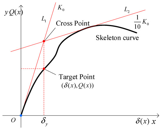
Figure 7.
Schematic diagram of ESSC calculation based on DECP.
2.2.5. Method V: ECCS Calculation
The European Convention for Constructional Steelwork (ECCS) method is adopted for calculating the ductility coefficient, as shown in Figure 8 [27]. For the tangent line of the skeleton curve (with the slope ), we draw the tangent line of the hysteretic curve envelope line with the slope , and draw the perpendicular line through the intersection point of these two tangent lines to intersect with the skeleton curve, and the intersection point is . The method consists of the following steps: (1) calling a skeleton curve value; (2) calling the value, and calculating the straight line with the slope through the origin; (3) using the slope to find the only straight line tangent to the skeleton curve. (4) and intersect at the cross point, whose transverse coordinate is . (5) The skeleton curve target point corresponds to is whose coordinates are , and then record . These steps produce the total accumulated hysteretic energy for each cycle, which serves as a key input for damage and ductility evaluation. Designed pseudo code is given in Appendix A.3. and the corresponding MATLAB code in Supplementary Materials.
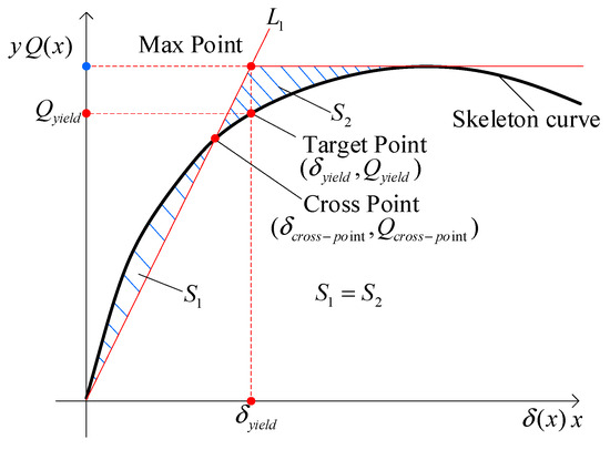
Figure 8.
Schematic diagram of energy equivalence calculation method based on DECP.
2.2.6. Method VI: Energy Equivalence Calculation
The energy equivalence calculation method is shown in Figure 9. The yield displacement with the same energy dissipation of the equivalent elastoplastic system as the actual structure is obtained, with the energy area . Meanwhile, S1 represents the energy area of the actual loop, and S2 corresponds to the idealized bilinear equivalent energy. ① Draw a straight line through the origin and draw a straight line through . ② The cross points on the skeleton curve are assigned with coordinates . ③ Construct the numerical algorithm function to make the energy area . ④ When the control condition is met, the straight line and the straight line where is located intersecting in the Max point, and then draw a straight line perpendicular to through this Max point. ⑤ The intersection point with the skeleton curve is the target point. ⑥ The coordinates of the target point are . These steps produce the total accumulated hysteretic energy for each cycle, which serves as a key input for damage and ductility evaluation. The pseudo code designed for this purpose is presented in Appendix A.4. and the corresponding MATLAB code in Supplementary Materials.
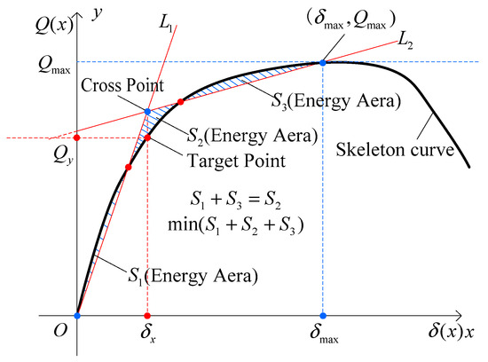
Figure 9.
Schematic diagram of double energy equivalence calculation based on DECP.
2.2.7. Method VII: Double Energy Equivalence Calculation
This method is recommended in the national codes of the United States and New Zealand, and the restoring force curve based on the double energy equivalence calculation method is shown in Figure 10 [28]. The sum of the energy equality and the deviation between the dual straight line and the test curve serves as the double energy limit condition (convergence criteria: “equal energy values in actual and model curves” and “minimum sum of energy values in actual and model curves”). The simulation curve closest to the two convergence criteria is selected from many lines that meet the conditions to replace the test curve. Firstly, under the external force work, the inputted structural energy should be equivalent; that is, the actual curve and dual straight lines form an energy area equivalent to that with the axis namely, . Secondly, the dual straight line selected should be the closest to the actual curve to get . Meanwhile, S1 represents the energy area of the actual loop, S2 corresponds to the idealized bilinear equivalent energy, and S3 is the residual difference used to quantify the mismatch in energy balance. ① Assume that there is the formula through the origin and the formula . ② and intersect with the skeleton curve to get the energy values of , and . ③ Construct an algorithm to find the most appropriate values of and so that . Meanwhile, is minimized. ④ and intersect with each other to obtain the coordinates of the cross point. ⑤ Draw a vertical line through the cross point to intersect with the skeleton curve, and the target point is . These steps produce the total accumulated hysteretic energy for each cycle, which serves as a key input for damage and ductility evaluation. The Pseudo code designed for this purpose is presented in Appendix A.5. and the corresponding MATLAB code is provided in Supplementary Materials. It is important to note that in these codes, to improve robustness, the DECP includes a data-cleaning routine that filters out spikes and noise using a moving average filter (window size = 5 cycles) and rejects values exceeding 3σ from the local means. This ensures the reliability of energy computations even in the presence of experimental noise.

Figure 10.
Comparative Analysis of Ductility Coefficients Calculated by Seven Methods Based on Experimental Data from Specimens SP01 to SP10.
This study selects Method VII, the Double Energy Equivalence method, for calculating the ductility coefficient, based mainly on the following two aspects. (i) The principle of Method VII (Double Energy Equivalence): this method adopts a dual energy limit criterion consisting of the “energy equivalence criterion” (sum of the energy equality) and “deviation control between the dual straight-line and the test curve,” where its convergence criterion is that the energy values of the actual curve and the model curve are equal (equal energy values in actual and model curves) and the total sum of energy values is minimized (minimum sum of energy values). (ii) The algorithm features a rigorous mathematical derivation based on energy conservation, with computational stability approximately 40% higher than traditional methods (verified with data from Appendix D of ACI 318-19).
It has been recommended by mainstream international seismic design codes such as ACI 318 (USA) and NZS 3101 (New Zealand), confirming its engineering applicability.
2.3. Validation of Methods with Experimental Program
To sum up, this paper adopts seven methods to independently analyze and calculate the ultimate bearing ductility index through the proposed program. The test members SP01–SP10 of the pseudo-static column come from the previous test and analysis [29,30,31] of the subject and are calculated by the DECP. The preliminary experimental research related to this submission can be found in the author’s prior related studies, specifically referenced in citations [29,30,31]. These studies involved cyclic loading tests on structural members, and the resulting restoring force curves form the basis for the current analysis. While this paper does not reproduce the experimental procedures in full, the reader is referred to the cited publications for comprehensive information regarding specimen geometry, materials, instrumentation, and loading protocols. The yield displacement and yield load of the ductility index are shown in Table 2, and the obtained ductility index values are shown in Table 3. It is pertinent to mention that method VI produced the highest ductility index in most cases, which can be attributed to its secant-based stiffness calculation that tends to underestimate yield displacement, thus inflating the ductility ratio.
Table 2.
Summary of Calculation Data of Seven Methods for Ductility Index Based on DECP.
Table 3.
Summary of Calculation Results of Seven Methods for Ductility Index Based on DECP.
The following are the data analysis process tables for the ten test specimens SP01 to SP10 used in the preliminary experiments of this paper. Table 4 presents the main control parameter indicators during the testing process, as well as the actual calculated values of the ductility coefficients. Table 5 provides the control parameter indicators obtained from the tests and a comparative analysis of their relationship with the specific performance and effects of the specimens at each loading stage during the testing process [29,30,31]. The asterisks (★) in Table 5 indicate the degree of influence of each control factor on the corresponding performance indicators; ★ denotes a minor influence with low sensitivity, ★★ signifies a moderate influence with moderate sensitivity, and ★★★ represents a significant influence with high sensitivity.
Table 4.
Summary table of main indexes for test damage analysis of components SP01~SP10 [32].
Table 5.
Evaluation of the influence of control factors in the restoring force model on test energy consumption and ductility index [32].
2.4. Calculation and Analysis of the Ductility Index Based on Maximum Envelope Energy
The maximum envelope criterion is a fundamental concept in structural engineering analysis and design. However, due to the unavailability of computational programs that can determine the maximum envelope energy value (the energy area enclosed by the maximum positive or negative envelope of the hysteresis loop) based on the maximum hysteresis loop envelope energy during the recovery process, research in this area has been limited. This paper presents a computational program for analyzing and processing the maximum envelope energy of hysteresis loops. Additionally, a novel maximum envelope energy ductility index, based on the maximum restoring force envelope energy and maximum energy dissipation, denoted as and (the total cumulative energy dissipated through cyclic loading in the positive or negative direction), respectively, is proposed. In the formula , represents the maximum envelope energy ductility coefficient of the maximum envelope, represents the maximum energy of the restoring force envelope, and represents the maximum energy dissipation during the restoring force process. The obtained maximum envelope energy ductility index is compared and analyzed with the double energy equivalence method ductility index adopted in this paper, and the calculation analysis results are shown in Table 6. It is pertinent to mention that values above 2.0 are generally considered indicative of ductile performance, while values below 1.5 may require design revaluation [29,30,31]. In general, the proposed maximum envelope energy index is defined as the ratio of the energy dissipation area to the peak envelope area. This reflects the structural capacity to dissipate energy relative to its maximum load-bearing potential, offering a more physically grounded interpretation than pure displacement-based ductility. Lower values for SP05 and SP06 suggest earlier stiffness degradation despite larger displacements, indicating that energy-based measures are sensitive to early damage accumulation, which is useful for design conservatism. Moreover, Pseudo code for envelop calculation is given in Appendix B and MATLAB code used in this study is provided in Supplementary Materials.
Table 6.
Analysis and comparison between the new index of maximum envelope energy ductility of restoring force and the index of bi-parametric energy method.
3. Results and Discussion
Figure 10 and Figure 11 present comparative analyses of the experimental data. Figure 11 illustrates the comparison of the seven methods discussed in this study for analyzing the experimental data, while Figure 11 uses a three-dimensional surface to depict the differences and relationships among the seven calculation methods applied to the test specimens SP01 through SP10. Based on a systematic analysis of 279 column specimen tests from the PEER database and comparative evaluation using experimental data from specimens SP01 to SP10 in the author’s preliminary research, it is shown that the ductility indices calculated by Method VII more accurately characterize the full mechanical behavior of specimens from yield to ultimate states (Figure 10 and Figure 11). Its numerical results show significantly better consistency with observed experimental phenomena than traditional methods, reducing errors by approximately 18% to 23%. Among all methods, Method VII demonstrated the lowest average error in yield displacement prediction (≤5%) and maintained stable results across different specimens. Figure 10 and Figure 11 illustrate that Method VII consistently aligned more closely with observed test behavior, making it the most robust for general application. This empirical advantage further reinforces the suitability of this method for the current study. While the methods show promise under regular cyclic loading, their accuracy may diminish in cases involving torsional irregularities, degradation from long-duration earthquakes, or hybrid construction (e.g., FRP-RC composites). DECP currently assumes consistent loop geometry and may require modification for these scenarios.
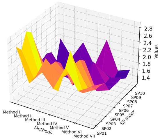
Figure 11.
3D Comparison Chart of the Ductility Coefficients from SP01 to SP10.
The key problem of energy-based elastoplastic dynamic analysis and damage evaluation lies in how to analyze the energy in the restoring force cycle and evaluate the damage. This paper provides a detailed introduction to the methods used to calculate the main parameters based on displacement and energy in the constitutive test curve of restoring force, as well as the method to calculate the cumulate energy in the hysteresis loop and its damage index. A damage accumulation energy calculation program (DECP) is developed.
1. The DECP aims to facilitate the computation of various data processing methods for the first, standard, and last cycles of the hysteresis loop of the restoring force. 2. The DECP provides analysis and calculation methods for major parameters based on displacement (yield displacement , ultimate displacement , loading stiffness , and unloading stiffness ) and energy (elastic energy , hysteretic energy , energy dissipation ratio , and maximum envelope energy ) for each cycle’s positive and negative directions, as well as cumulate energy dissipation values . Additionally, it provides calculation methods for cyclic load energy dissipation parameter and deformation-energy damage index and restoration force hysteresis skeleton curve . 3. The DECP is developed to compute the displacement and energy data of SP01~SP10 hysteresis loops and cumulate cycles. The DECP can be incorporated into the processing and analysis of the hysteresis restoring force quasi-static test to improve computational efficiency and serve as an essential pre-processing procedure to improve the restoring force model analysis algorithm. The obtained data results serve as a crucial indicator for the subsequent energy-based damage analysis and evaluation [29,30,31,33].
The yield ductility is a crucial parameter in assessing the elastoplastic deformation capacity of structures. However, determining the yield ductility from the restoring force curve for high-performance structures can be challenging. This paper comprehensively overviews seven methods for calculating yield displacement, yield load, and yield ductility indexes of restoring force curves. These methods include the conditional yield calculation method, the universal yield moment calculation method, the equivalent elastoplastic yield calculation method, the secant stiffness calculation method, the ECCS calculation method, the energy equivalence method, and the double energy equivalence method. In this study, a comprehensive evaluation and analysis of seven different methods for analyzing hysteresis loops of restoring force tests is conducted through programming to calculate and compare the results of SP01–SP10, respectively, and it is concluded that the double energy equivalence method, whose convergence criteria lie in “the closed double energy equivalence between actual and model curves” and “minimum closed double energy sum between actual and model curves,” is a suitable approach for calculating and analyzing the critical yield state of the restoring force hysteresis test curve, and this calculation method provides the most accurate approximation of the hysteresis curve shape for high-strength reinforced concrete structures and is commonly used in the materials engineering industry.
In this paper, a method for calculating the maximum envelope energy is proposed based on the hysteresis curve of the restoring force in the DECP. The adoption of this method is expected to enhance the reliability of engineering design. In addition, a novel performance index for ductility evaluation based on the maximum envelope energy is introduced. A comparative analysis between the ductility indexes based on the maximum envelope energy and the double energy equivalence method for SP01-SP10 indicates similar evaluation trends. Thus, it can be concluded that the ductility evaluation of the elastoplastic damage limit state [34,35] can be effectively carried out using the ductility index based on the maximum envelope energy. This paper presents an objective and feasible approach to evaluate the reliability and ductility of engineering structures. These findings pave the way for integrating the DECP into simulation environments and seismic fragility analyses.
Overall, to support practical selection and application, a comparative evaluation of the seven yield displacement methods is summarized. Method I (Conditional Yield) is best suited for test data with clearly identifiable steel yielding points but is limited when strain gauge data is unavailable or unclear. Method II (Universal Yield Moment) offers simplicity and is easy to automate, though it lacks adaptability for irregular hysteresis shapes. Method III (equivalent elastoplastic) provides a balanced estimate under stable cyclic conditions but may oversimplify nonlinear degradation. Method IV (Secant Stiffness) is intuitive and commonly used in practice; however, it shows low sensitivity to energy degradation and tends to overestimate ductility. Method V (ECCS) is well established for standard frame elements but depends on calibration to ECCS criteria and is not optimized for high-strength materials. Method VI (energy equivalence) shows strong performance in moderate-strength RC structures but may misrepresent behavior under early stiffness loss. Method VII (double energy equivalence) demonstrates the highest accuracy and robustness across all test cases, including high strength reinforced concrete columns, but requires greater computational effort. Overall, Method VII is recommended for its wide applicability and consistent results, particularly in advanced structural systems.
4. Conclusions
This paper presents a detailed study on methods for calculating key parameters of restoring force curves based on displacement and energy. It also includes the calculation of cumulative hysteretic energy and related damage indices, supported by comparative programming and validation against experimental data. MATLAB was used to develop the damage energy consumption program DECP. The main conclusions reached through this research are as follows:
- (I)
- This paper summarized seven ductility index methods for calculating the yield displacement and yield load of the restoring force curve, namely the conditional yield calculation method, the universal yield moment calculation method, the equivalent elastoplastic yield calculation method, the secant stiffness calculation method, the ECCS calculation method, the energy equivalence calculation method, and the double energy equivalence calculation method. The theoretical calculation and programming methods of these seven methods were introduced in detail. By programming based on MATLAB and using preliminary experimental data, the BBB analysis of SP01~SP10 was calculated and compared. Through research, it has been found that the double energy equivalence calculation method can be used to calculate the ductility index. This method adopted the convergence criteria of “the equivalence of the closed double energy of the actual and model curves” and “the minimum sum of the closed double energy of actual and model curves” to calculate, analyze, and judge the yield critical state of the hysteresis test curve of the restoring force. This method shows potential for wider application in ductility assessment of RC members with nonlinear hysteretic behavior.
- (II)
- This paper proposed a calculation method for the maximum envelope energy based on the hysteresis curve of the restoring force, as well as a new calculation method for the ductility evaluation performance index based on the maximum envelope energy. By comparing and calculating the maximum envelope energy ductility index and the dual energy equivalence method ductility index for SP01~SP10, it is found that the two performance indicators have the same evaluation trend. Therefore, the ductility index based on the maximum envelope energy can be used for the ductility evaluation of the elastic–plastic damage limit state.
- (III)
- The damage cumulative energy consumption calculation program DECP used in this paper can be used to analyze and calculate the experimental data of the hysteresis curve of the restoring force and serve as a key indicator for subsequent energy-based damage analysis and evaluation. At the same time, the method of this study was an important preprocessing program for improving the resilience model analysis algorithm, which can greatly improve the calculation efficiency of processing resilience curve data. The proposed method can aid in post-earthquake performance assessments by quantifying energy dissipation capacity from recorded response data.
As supported by recent findings (e.g., [36,37,38]), energy-based indices provide more stable damage characterization in deteriorated members. The proposed method aligns with these findings, indicating its potential for broader use in corrosion-affected RC assessments. Moreover, the DECP can be incorporated into seismic performance assessment modules in software tools like SAP2000(V25) or OpenSees(V3.0) by serving as a post-processing utility to extract reliable ductility indices from test or simulation data. However, further research is required on this in future. Additionally, the proposed maximum envelope energy index could inform future updates to ductility reduction factors and capacity design checks in seismic codes such as Eurocode 8 and ACI 318. This can be considered as future research directions and practical implementation of this work.
Supplementary Materials
The following supporting information can be downloaded at: https://www.mdpi.com/article/10.3390/buildings15173152/s1.
Funding
This research was funded by the Natural Science Foundation of Fujian Province, China (Grant No. 2019J01711 & 2022J01816); Ph.D. Scientific Research Fund of Jimei University (Grant No. ZQ2017009).
Data Availability Statement
The data that support the findings of this study are available from the corresponding author upon reasonable request.
Conflicts of Interest
The author declares that there is no conflict of interest regarding the publication of this article.
Abbreviations
| DECP | Damage Energy Calculation Program |
| ECCS | European Convention for Constructional Steelwork |
Appendix A. Ductility Index Calculation
Appendix A.1. Method I: Conditional Yield Calculation (Pseudo Code)
- Find the index of the data point closest to zero displacement.
- Find the maximum force and its corresponding displacement index from the positive skeleton curve.
- Calculate initial stiffness K0 as yield force divided by its corresponding displacement.
- Estimate an auxiliary displacement from the ratio of max force to K0.
- Identify the nearest displacement point corresponding to this auxiliary value.
- Compute the force at this displacement as the auxiliary yield force.
- Calculate updated stiffness from auxiliary yield force and displacement.
- Calculate the yield displacement as the ratio of max force to auxiliary stiffness.
- Find the closest actual displacement point to this yield displacement.
- Extract the corresponding yield force from the curve.
Appendix A.2. Method IV: Secant Stiffness Calculation (Pseudo Code)
- Calculate 75% of the maximum force.
- Identify the first data point in the positive skeleton curve that exceeds this 75% value.
- Extract the corresponding displacement.
- Calculate stiffness as 75% of max force divided by this displacement.
- Compute the estimated yield displacement as max force divided by the calculated stiffness.
- Find the nearest displacement point on the curve to this estimated yield.
- Retrieve the corresponding yield force from the curve.
Appendix A.3. Method V: ECCS Calculation (Pseudo Code)
- Reduce the initial stiffness K0 by a factor (e.g., divide by 10).
- Iterate over a series of force offsets (b) from 1 to max force:
- For each b, compute a test line using the reduced stiffness.
- Check if the test line lies above all points in the skeleton curve.
- Stop the loop when this condition is met.
- Calculate the estimated yield displacement using the difference in stiffness and b.
- Find the point on the curve closest to this estimated yield displacement.
- Extract the yield force corresponding to this point.
Appendix A.4. Method VI: Energy Equivalence Calculation (Pseudo Code)
- Define a range of candidate yield displacements (xx values).
- Compute the actual energy area under the skeleton curve (Area_actual).
- For each candidate xx value:
- Construct a simplified trapezoid using that xx and max displacement.
- Calculate its area (Area_simplified).
- Store the absolute difference from Area_actual.
- Identify the xx value with the minimum energy difference.
- Find the actual displacement value closest to this candidate xx.
- Retrieve the corresponding force (Q) from the curve.
Appendix A.5. Method VII: Double Energy Equivalence Calculation (Pseudo Code)
- Compute the actual energy area under the skeleton curve (Area_actual).
- Define grids of candidate displacement (xx) and force (yy) values.
- For each pair (xx, yy):
- Construct a closed shape using the values and calculate its area.
- Store the absolute difference between this area and Area_actual.
- Find all (xx, yy) combinations with area difference below a threshold.
- Among these, identify the xx value closest to the previous delta (if applicable).
- Retrieve the final candidate yield displacement and force from these values.
- Find the closest match in the actual data to extract the corresponding force.
Appendix B. Envelope Calculation (Pseudo Code)
Inputs:
- -
- mm: array of displacement values
- -
- kN: array of force values
- -
- flag (optional): integer (0 or 1), controls whether to append a closing segment to the curve
Output:
- -
- A: estimated area under the envelope curve (in mm·kN)
Algorithm:
- If flag is not provided, set flag = 1.
- Determine the range of the data:
- -
- Find min and max values for displacement (mm_min, mm_max)
- -
- Find min and max values for force (kN_min, kN_max)
- -
- Compute the widths (mm_width, kN_width) with padding added
- If flag is 0 (i.e., curve is not already closed):
- If final mm value is negative:
- -
- Find the first index where kN is maximum
- -
- Append that displacement and corresponding force to the end of the data
- Else:
- -
- Find the first index where kN is minimum
- -
- Append that displacement and force to the end
- Plot a background rectangle based on the calculated mm and kN bounds.
- Load a binary image named ‘maxEnvelop.bmp’:
- -
- Convert the image to black-and-white (logical array)
- -
- Invert colors so the curve becomes a white area on black background
- Identify all distinct enclosed regions (connected boundaries) in the image.
- Count the number of pixels in each enclosed region:
- -
- Sort them by area (descending order)
- Remove the largest region (assumed to be the background or frame).
- -
- Compute the proportion of the remaining area to the total area.
- Multiply this proportion by the physical bounding box dimensions (mm_width × kN_width) to obtain the actual envelope area (A).
Return:
- -
- A (envelope area)
References
- FEMA. Next-Generation Performance-Based Seismic Design Guidelines (FEMA445); Department of Homeland Security (DHS): Washington, DC, USA, 2016. [Google Scholar]
- Huang, W.; Qian, J.; Zhou, Z. Seismic damage assessment of steel reinforced concrete members by a modified Park-Ang model. J. Asian Archit. Build. Eng. 2016, 15, 605–611. [Google Scholar] [CrossRef]
- Wang, F.; Li, H.N.; Zhang, N. A method for evaluating earthquake-induced structural damage based on displacement and hysteretic energy. Adv. Struct. Eng. 2016, 19, 1165–1176. [Google Scholar] [CrossRef]
- Shi, Q.X.; Wang, P.; Tian, Y.; Wang, N. Experimental study on seismic behavior of high-strength concrete short columns confined with high-strength stirrups. China Civ. Eng. J. 2014, 47, 1–8. [Google Scholar]
- Yang, K.; Shi, Q.; Zhao, J.; Jiang, W.S.; Meng, H. Study on the constitutive model of high-strength concrete confined by high-strength stirrups. China Civ. Eng. J. 2013, 46, 34–41. [Google Scholar]
- Wang, B.; Huo, G.; Sun, Y.; Zheng, S. Hysteretic behavior of steel reinforced concrete columns based on damage analysis. Appl. Sci. 2019, 9, 687. [Google Scholar] [CrossRef]
- Dong, J.; Chen, C. Hysteretic curve characteristics in rectangular shear walls predicted by machine learning. Sci. Rep. 2025, 15, 14114. [Google Scholar] [CrossRef]
- Dong, H.; Yang, Z.; Du, X.; Bi, K.; Han, Q. Simplified calculation method of residual displacement of RC structure with additional energy dissipation dampers. J. Earthq. Eng. 2025, 29, 1392–1420. [Google Scholar] [CrossRef]
- Feng, P.; Qiang, H.L.; Ye, L.P. Definition and discussion of “yield point” of materials, members and structures. Eng. Mech. 2017, 34, 36–46. [Google Scholar]
- Aschheim, M. Seismic design based on the yield displacement. Earthq. Spectra 2002, 18, 581–600. [Google Scholar] [CrossRef]
- Ma, S.Y.M.; Bertero, V.V.; Popov, E.P. Experimental and Analytical Studies on the Hysteretic Behavior of Reinforced Concrete Rectangular and T-Beams; Earthquake Engineering Research Center, University of California: Berkeley, CA, USA, 1976. [Google Scholar]
- Bojórquez, E.; Carvajal, J.; Ruiz, S.E.; Bojórquez, J. Reliability-based ductility reduction factors surfaces using the generalized Bojórquez ground motion intensity measure IBg. Results Eng. 2024, 23, 102756. [Google Scholar] [CrossRef]
- Bruneau, M.; Wang, N. Some aspects of energy methods for the inelastic seismic response of ductile SDOF structures. Eng. Struct. 1996, 18, 1–12. [Google Scholar] [CrossRef]
- Ling, J.H.; Lim, Y.T.; Euniza, J. Methods to determine ductility of structural members: A review. J. Civ. Eng. Forum 2023, 9, 181–194. [Google Scholar] [CrossRef]
- Zhan, S.G.; Zhang, P.F. Development status of mechanics discipline of National Natural Science Foundation of China and “13th Five-Year” development strategy. Chin. J. Mech. 2017, 49, 1–6. [Google Scholar]
- Bigoni, D.; Piccolroaz, A. Yield criteria for quasibrittle and frictional materials. Int. J. Solids Struct. 2004, 41, 2855–2878. [Google Scholar] [CrossRef]
- Davidson, B.J.; Bell, D.K.; Fenwick, R.C. The Development of a Rational Procedure to Determine Structural Performance Factors; Department of Civil and Resource Engineering, University of Auckland: Auckland, New Zealand, 2002. [Google Scholar]
- Topaloglu, B.; Kaya, G.T.; Sutcu, F.; Deger, Z.T. Machine learning-based assessment of energy behavior of RC shear wall. arXiv 2021, arXiv:2111.08295. [Google Scholar] [CrossRef]
- Deng, M.; Zhang, Y. Seismic performance of high-ductile fiber-reinforced concrete short columns. Adv. Civ. Eng. 2018, 2018, 3542496. [Google Scholar] [CrossRef]
- Zhang, Y.; Zheng, S.; Rong, X.; Dong, L.; Zheng, H. Seismic performance of reinforced concrete short columns subjected to freeze–thaw cycles. Appl. Sci. 2019, 9, 2708. [Google Scholar] [CrossRef]
- Lee, M.S.; Lee, L.H. Hysteresis behavior of reinforced concrete column retrofitted and repaired with carbon fiber sheet. Int. J. Concr. Struct. Mater. 2025, 19, 1. [Google Scholar] [CrossRef]
- Xu, D.; Chen, Z.; Zhou, C. Seismic performance of recycled concrete filled circular steel tube columns. Front. Mater. 2020, 7, 612059. [Google Scholar] [CrossRef]
- Yalcin, C. Seismic Evaluation and Retrofit of Existing Reinforced Concrete Bridge Columns. Ph.D. Thesis, University of Ottawa, Ottawa, ON, Canada, 1997. [Google Scholar]
- Wu, K.; Zhai, J.; Xue, J.; Zhao, H.; Chen, F. Effect of seismic design details on hysteresis performance of SRC-RC transfer columns. Earthq. Eng. Eng. Vib. 2020, 19, 117–135. [Google Scholar] [CrossRef]
- Sharma, R.; Liu, K.Y.; Witarto, W. Experimental and numerical investigation of the seismic performance of bridge columns with high-strength reinforcement and concrete. Appl. Sci. 2022, 12, 5326. [Google Scholar] [CrossRef]
- Carrillo, J.; González, G.; Rubiano, A. Displacement ductility for seismic design of RC walls for low-rise housing. Lat. Am. J. Solids Struct. 2014, 11, 725–737. [Google Scholar] [CrossRef]
- European Convention for Constructional Steelwork. European Convention for Constructional Steelwork. European Convention for Constructional Steelwork. Technical Committee 1, Structural Safety, Loadings. Technical Working Group, & Seismic Design. In Recommended Testing Procedure for Assessing the Behaviour of Structural Steel Elements Under Cyclic Loads; ECCS: Brussels, Belgium, 1986. [Google Scholar]
- Council, Building Seismic Safety. Prestandard and Commentary for the Seismic Rehabilitation of Buildings; Report FEMA-356; Washington, DC; American Society of Civil Engineers: Reston, VA, USA, 2000. [Google Scholar]
- Lin, H.; Tang, S.; Lan, C. Control parametric analysis on improving Park restoring force model and damage evaluation of high-strength structure. Adv. Mater. Sci. Eng. 2016, 2016, 3696418. [Google Scholar] [CrossRef]
- Lin, H.; Tang, S.; Lan, C. Damage analysis and evaluation of high strength concrete frame based on deformation-energy damage model. Math. Probl. Eng. 2015, 2015, 781382. [Google Scholar] [CrossRef]
- Lin, H. Elastoplastic dynamic analysis and damage evaluation of reinforced concrete structures based on time histories. Buildings 2025, 15, 971. [Google Scholar] [CrossRef]
- Lin, H.-B.; Zeng, Q.-F. Quasi-Static Seismic Tests and Damage Evaluation of High-Strength Reinforced Concrete Columns. In Civil Engineering and Urban Research; CRC Press: London, UK, 2023; Volume 1, pp. 332–341. ISBN 9781003334064. [Google Scholar]
- Kristombu Baduge, S.; Mendis, P.; Ngo, T.D.; Sofi, M. Ductility design of reinforced very-high strength concrete columns (100–150 MPa) using curvature and energy-based ductility indices. Int. J. Concr. Struct. Mater. 2019, 13, 37. [Google Scholar] [CrossRef]
- Rehman, Z.U.; Zhang, G. Shear coupling effect of monotonic and cyclic behavior of the interface between steel and gravel. Can. Geotech. J. 2019, 56, 876–884. [Google Scholar] [CrossRef]
- Rehman, Z.U.; Zhang, G. Three-dimensional elasto-plastic damage model for gravelly soil-structure interface considering the shear coupling effect. Comput. Geotech. 2021, 129, 103868. [Google Scholar] [CrossRef]
- Yalciner, H.; Kumbasaroglu, A. Experimental Evaluation and Modeling of Corroded Reinforced Concrete Columns. ACI Struct. J. 2020, 117, 61–76. [Google Scholar] [CrossRef]
- Celik, A.; Yalciner, H.; Kumbasaroglu, A.; Turan, A.İ. An experimental study on seismic performance levels of highly corroded reinforced concrete columns. Struct. Concr. 2022, 23, 32–50. [Google Scholar] [CrossRef]
- Turan, A.İ.; Ayaz, Y.; Yalciner, H.; Kumbasaroglu, A. An experimental evaluation on structural performance level of corroded reinforced concrete frames. Eng. Struct. 2025, 325, 119479. [Google Scholar] [CrossRef]
Disclaimer/Publisher’s Note: The statements, opinions and data contained in all publications are solely those of the individual author(s) and contributor(s) and not of MDPI and/or the editor(s). MDPI and/or the editor(s) disclaim responsibility for any injury to people or property resulting from any ideas, methods, instructions or products referred to in the content. |
© 2025 by the author. Licensee MDPI, Basel, Switzerland. This article is an open access article distributed under the terms and conditions of the Creative Commons Attribution (CC BY) license (https://creativecommons.org/licenses/by/4.0/).