Article

Study on the Empirical Probability Distribution Model of Soil Factors Influencing Seismic Liquefaction

1
State Key Laboratory of Simulation and Regulation of Water Cycle in River Basin, China Institute of Water Resources and Hydropower Research, Beijing 100038, China
2
Engineering Research Center on Anti-Earthquake and Emergency Support Techniques of Hydraulic Projects, Ministry of Water Resources, Beijing 100048, China
3
Yellow River Engineering Consulting Co., Ltd., Zhengzhou 450052, China
*
Author to whom correspondence should be addressed.
Buildings 2025, 15(16), 2861; https://doi.org/10.3390/buildings15162861
Submission received: 25 June 2025 / Revised: 2 August 2025 / Accepted: 8 August 2025 / Published: 13 August 2025
(This article belongs to the Section Building Structures)

Abstract

One of the important tasks in sand liquefaction assessment is to evaluate the likelihood of soil liquefaction. However, most liquefaction assessment methods are deterministic for influencing factors and fail to calculate the liquefaction probability by systematically considering the probability distributions of soil factors. Based on field liquefaction investigation cases, probability distribution fitting and a hypothesis test were carried out. For the variables that failed to pass the fitting and test, the kernel density estimation was conducted. Methods for calculating the liquefaction probability using a Monte Carlo simulation with the probability distribution were then proposed. The results indicated that for (N1)60, SM, S, and GM followed a Gaussian distribution, while CL and ML followed a lognormal distribution; for FC, SM and GM followed a lognormal distribution; and for d50, ML and S followed a Gaussian and lognormal distribution, respectively. The other factors’ distribution curves can be calculated by kernel density estimation. It is feasible to calculate the liquefaction probability based on a Monte Carlo simulation of the variable distribution. The result of the liquefaction probability calculation in this case was similar to that of the existing probability model and was consistent with actual observations. Regional sample differences were considered by introducing the normal distribution error term, and the liquefaction probability accuracy could be improved to a certain extent. The liquefaction probability at a specific seismic level or the total probability within a certain period in the future can be calculated with the method proposed in this paper. It provides a data-driven basis for realistically estimating the likelihood of soil liquefaction under seismic loading and contributes to site classification, liquefaction potential zoning, and ground improvements in seismic design decisions. The practical value of seismic hazard mapping and performance-based design in earthquake-prone regions was also demonstrated.

1. Introduction

Soil seismic liquefaction generally refers to the process in which the pore water pressure increases and the effective stress decreases under seismic loading, and ultimately, the soil loses its shear strength, behaving in a manner similar to liquid [1,2]. Sand boiling, ground fissures, lateral spreading, and settlement may occur after liquefaction, posing serious threats to overlying structures [3]. The first step is to analyze whether liquefaction will occur in the study of soil seismic liquefaction, which is known as a liquefaction assessment. An accurate liquefaction assessment is of paramount importance for practical engineering applications [4,5,6].
Methods for liquefaction assessments commonly include deterministic and probabilistic approaches. The earliest deterministic methods were developed by Seed et al., who conducted a liquefaction mechanism analysis. Subsequent research has continued to develop and refine this method based on these studies, finally culminating in the simplified method in 1984 [7]. The principles of this method are as follows: based on seismic loading and field investigation data, the seismic shear stress (CSR) and soil resistance (CRR) are calculated and then compared. If the CSR exceeds the CRR, soil liquefaction is deemed to have occurred. This method is straightforward, easy to apply, and has been widely used [8,9,10]. Mainstream deterministic liquefaction assessment methods worldwide are largely based on this approach, tailored to local conditions and practical contexts [11,12,13].
Design goals are given in terms of probability levels in current seismic safety assessments for engineering sites, while the deterministic liquefaction assessment method can only provide the answer of yes or no, which make it incompatible with the current performance-based seismic analysis requirements [3]. In addition, due to the variability in soil properties, the probabilistic nature of seismic events, and various experimental errors introduced during the determination of soil properties, uncertainties are inevitably introduced into the soil liquefaction assessment [14,15,16]. Soil liquefaction essentially is a probabilistic issue, necessitating probabilistic methods to address the aforementioned uncertainties to match the existing performance-based seismic engineering design [17,18,19,20]. With the continuous accumulation of field liquefaction investigation cases, particularly from the widely used standard penetration test (SPT), a large amount of experimental data has been accumulated. Numerous empirical equations and models have been developed based on SPT data, and it has become the most commonly used probabilistic liquefaction assessment method.
The probabilistic assessment method based on SPT data was initially developed in 1988. Field investigation cases were collected by Liao et al. [21], and a regression analysis was performed to derive liquefaction assessment curves at different probability levels, thereby introducing probabilistic means for liquefaction assessments. Subsequently, Yang et al. [22], Zhao et al. [23], and Hu and J. Wang [24] continuously expanded the seismic liquefaction case database and incorporated probabilistic statistical methods, including Bayesian updating, to develop various probabilistic assessment methods. However, those research studies still treated influencing factors as fixed values during their calculations, and probabilistic means were determined only through probability theory.
Cruz et al. [25] reviewed the assessment methods to calculate liquefaction probability and presented a performance-based seismic engineering design through a full-probability liquefaction hazard assessment at the same time. However, they failed to establish it from the perspective of the probabilistic distribution, and the calculation process was not combined with soil factor distributions. Sianko et al. [26] established seismic liquefaction vulnerability curves considering the uncertainty of dynamic loading through a Monte Carlo simulation. The Monte Carlo method was employed by Wang et al. to sample anisotropic random fields to analyze the influence of the spatial variability of clay soil [27]. Fragility curves and probabilistic risk analyses were employed by Sherzer et al. to provide a structured framework for the comprehensive assessment of risks [28]. Huang and G. S. Wang [29] developed an empirical probabilistic distribution method of liquefied soil layer thickness and compared the mean values and standard deviations of probabilistic distributions in different regions, but they also ignored the soil factors’ influence. Wang et al. provided new insights into the landslide mechanism of discontinuous rock slopes by introducing a mixed cohesive phase-field numerical method [30]. Urlainis et al. proposed a comprehensive framework for a multi-hazard risk assessment and the management of mitigation strategies as a decision support tool for extreme events [31]. Few studies have been conducted on the liquefaction probability assessment method by systematically considering the probability distribution of soil factors [32,33].
The SPT data of field liquefaction investigation cases from various countries and regions were collected and analyzed. Probability distribution fitting and a hypothesis test of soil factors were carried out. For the variables that failed to pass the fitting and hypothesis testing, a kernel density estimation was conducted. The methods for calculating the liquefaction probability using a Monte Carlo simulation with the probability distribution were then proposed in this paper. The validity of the proposed method was verified through practical case calculations, and the factors influencing the sensitivity were analyzed. The regional differences of the samples and the method, which can be further studied and improved in the future, were also discussed. The overall research framework is illustrated in Figure 1. The research results can provide a reference for seismic liquefaction probability assessments.

2. Analysis of Liquefaction Influencing Factors and the Collection and Processing of Field Liquefaction Investigation Cases

2.1. Analysis of Soil Properties via Liquefaction Influencing Factors

The contact stress between soil particles is altered under cyclic shearing or the repeated vibration caused by seismic motion [1]. It disrupts the original soil structural state and causes the particles to lose contact with each other once the stress reaches a certain threshold. At the same time, the stress previously transmitted through contact points between soil particles is transferred to the pore water, leading to an increase in the pore water pressure. As the number of cycles increases, the pore water pressure gradually accumulates and rises. Liquefaction occurs when the pore water pressure increases to the level of the overburden pressure [2]. Soil liquefaction is a complex phenomenon; its initiation, development, and dissipation are constrained by the physical properties, stress conditions, and boundary conditions. Many factors influence this process, which can be divided into the following three categories: dynamic loading, environmental factors, and soil factors. The influencing factors adopted in various liquefaction evaluation methods typically include deterministic, probabilistic, and machine learning methods. They have been systematically reviewed and are compiled in Table 1, where M is the magnitude; M is the peak acceleration; M is the epicentral distance; ds is the depth; dw is the groundwater table; σ is the total stress; σ’ is the effective stress; (N1)60 is the corrected standard blow count; FC is the fine content; DR is the relative density; d50 is the average particle size; N is the standard blow count; ρc is the clay content; ED is the earthquake duration; and ST is the soil type.
In Table 1, the representative factors of the three aspects in previous research are considered. All three types of factors were taken into account when the above methods were established, but the specific number of factors varied. Some studies have regarded seismic loads and environmental factors as random variables and used their respective probability distributions to calculate the liquefaction probability. However, in the existing research, soil factors are mostly treated as deterministic and directly substituted into the calculation; the uncertainties are ignored. Few studies have incorporated the probability distribution of soil factors into the calculation of the liquefaction probability, which requires further exploration. There are many factors influencing soil liquefaction, such as soil density, structure, saturation, gradation characteristics, permeability, stress state, and dynamic load characteristics, and the relationships among them are complex [34,35,36]. Among these, factors related to soil properties include the fine content, particle gradation, consolidation degree, compaction, relative density, particle shape, saturation, plasticity index, and the original in situ structure [37].
The fine content influences the permeability and pore water pressure dissipation, thereby increasing the liquefaction risk [34,38]. Particle gradation influences the wide distribution of particle sizes; a more compact structure can be formed, which improves the shear strength and stability of the soil mass, thus reducing the liquefaction potential [39]. Consolidation influences the particle structure; loose soil particles are more likely to be rearranged and the pore water pressure is more likely to accumulate under dynamic loading, which leads to an increased probability of liquefaction [40]. Relative density is also an important factor for measuring the compactness, which is closely related to the liquefaction potential [41]. Particles with sharp edges and corners, rough surfaces, and irregular shapes are able to form stronger inter-particle interlocking and frictional forces, thereby enhancing the shear strength of the soil and reducing the liquefaction risk [42]. Saturation is one of the key factors influencing the soil liquefaction potential [43]. When the soil is fully saturated (with a saturation degree close to 100%), the pore water pressure can be rapidly increased and is difficult to dissipate, leading to an obvious reduction in the effective stress and a substantial increase in the likelihood of liquefaction. The plasticity index reflects the content of the cohesive components and has a significant impact on the liquefaction potential [44]. Soil with a strong in situ structure exhibits a higher density and shear strength. It can better resist particle rearrangement and pore water pressure increases under dynamic loading. However, when the soil is disturbed or damaged, the in situ structure may be weakened, leading to a significant decrease in liquefaction resistance [45].
In summary, there are numerous soil-related factors that influence seismic liquefaction. The relationships between these factors and liquefaction are highly complex. It is necessary to consider both the representativeness of factors and the data availability in the actual experiments. Otherwise, using the established liquefaction assessment method, it may be difficult to calculate the liquefaction probability accurately. Therefore, it is extremely difficult to fully consider all these factors when establishing the probability assessment method. Currently, seismic liquefaction probability calculation methods mainly rely on field liquefaction case databases, among which the standard penetration test (SPT) is the most commonly used method due to its simple operation, mature testing technology, and sufficient accumulated data [23]. SPT data generally contain the parameters including the corrected SPT blow count ((N1)60), fine content (FC), and average particle size (d50). (N1)60 can reflect the soil’s compactness and relative density to some extent [24]. FC, and d50 can reflect the particle gradation and the particle characteristics, etc. Factors such as particle gradation, particle shape, and in situ structure are difficult to directly quantify. There were only limited data on factors such as consolidation degree, compactness, relative density, saturation, and plasticity index, which were hardly enough for a statistical analysis and even increased the statistical error. In this paper, (N1)60, FC, and d50 are selected as representative soil factors to develop a new probabilistic assessment method.

2.2. Collection and Processing of Field Liquefaction Investigation Cases Based on SPT

Historical data from 55 seismic liquefaction cases were collected from the liquefaction databases established by Cetin [8], Seed [7], and Hu [34], and spanning the period from 1802 to 2023, with a total of 749 sample data. These samples covered regions including China, Japan, the United States, Australia, New Zealand, etc., essentially representing the major high-seismicity zones around the world. Existing research indicates that liquefaction generally does not occur when the magnitude is less than five. However, deep-buried sandy soil still has the possibility of liquefaction, and there are cases of liquefaction in sandy soil, fine silt, and even gravelly soil [8]. All selected cases are associated with earthquakes of a magnitude of 5.0 or higher. The dataset includes records from earthquakes such as the New Zealand and Jiji events, with some samples’ depths exceeding 20 m. The soil types covered are diverse, including sandy soils, silt, and fine sands. Compared to the datasets originally adopted by Seed et al. in their seminal liquefaction evaluation studies, the dataset used in this study provides improved representativeness and broader soil coverage [8].
Descriptive statistics were determined for the collected SPT liquefaction data to analyze the value range and dispersion degree of each variable to have a clear understanding of the data distribution. The results are illustrated in Table 2. S is sand, SM is silty sand, CL is low-plasticity clay, ML is low-plasticity silt, and GM is gravelly soil. The soil classification used in this study follows the approach proposed by Hu et al., in which soil types are categorized using Unified Soil Classification System (USCS) group symbols (e.g., S, SM, CL, ML, and GM) [34]. It can be seen that there is a variation to a certain extent under different soil type conditions, which indicates that outliers exist in the collected data. The large variability would reduce the parameters’ statistical effect and even lead to a loss in statistical meaning, demonstrating that the data need to be further processed.
The purpose of data preprocessing was to eliminate outliers for each variable. In the studies related to soil properties in geotechnical engineering, it is generally assumed that certain characteristics of the same soil type should exhibit similar patterns. However, in practical observations, anomalies often occur due to factors such as measurement errors, data entry mistakes, or extreme geological conditions that deviate from the target soil type. If such data points are not properly addressed, this may lead to skewed parameter distributions during fitting processes, with extreme values dominating the model results. In severe cases, it can even cause distribution models to fail to converge or fit properly.
Therefore, removing data points that significantly deviate from the overall characteristics helps restore the true distribution pattern of soil parameters and enhances the representativeness and stability of the probability model. In geotechnical engineering research, it is recommended to adopt the box plot method based on the interquartile range (IQR) to identify and remove outliers [34]. Previous studies have showed that it has good stability and applicability in processing on-site measured soil property data.
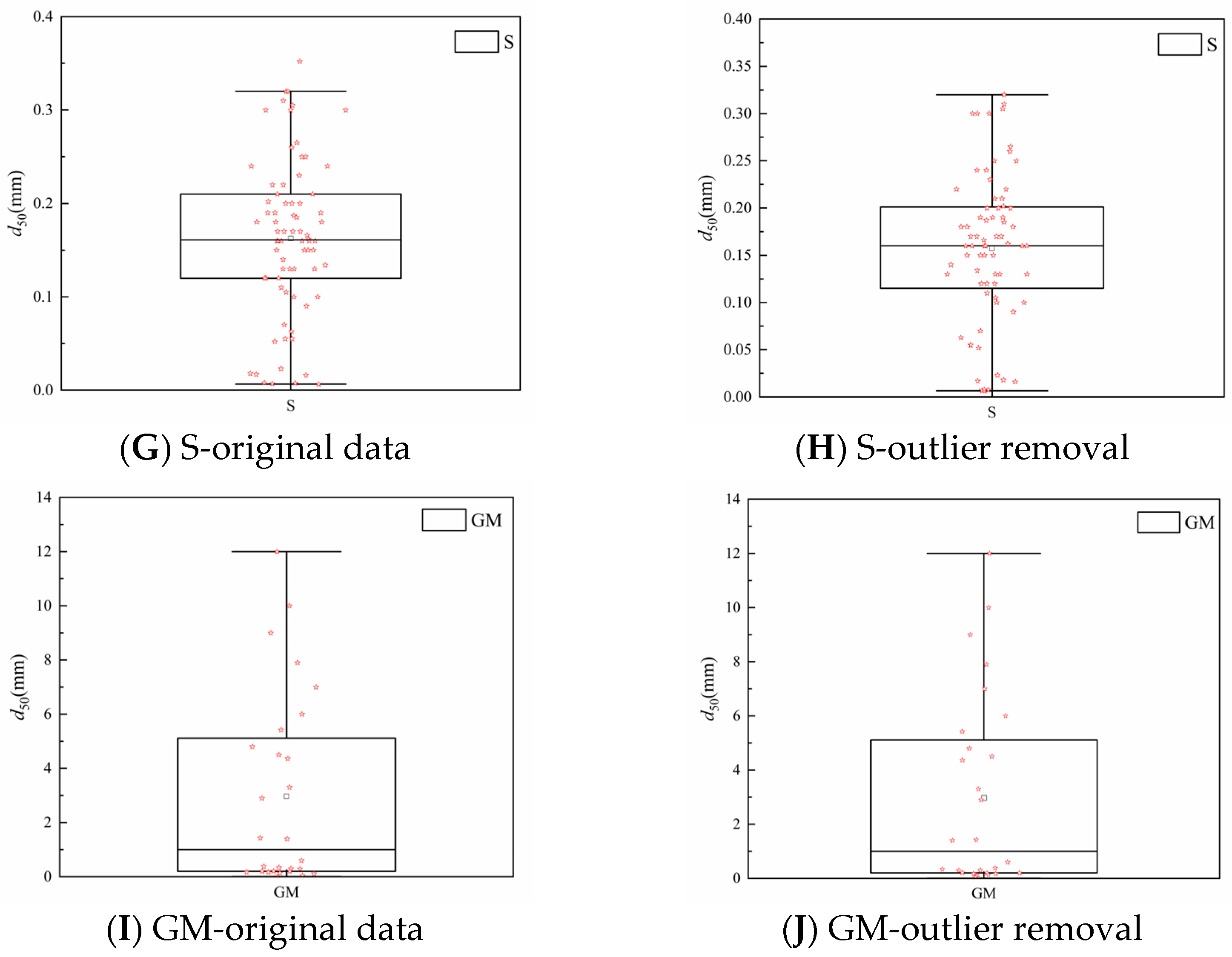
The box plot method, based on the interquartile range (IQR), was employed to detect and remove outliers from the dataset in this paper. The IQR is defined as the distance between the third quartile (Q3) and the first quartile (Q1), representing the range within which the middle 50% of the data lie. According to classical statistical theory, data points falling outside the interval Q1 − 1.5 × IQR, Q3 + 1.5 × IQR are considered outliers, as they deviate significantly from the central tendency of the dataset. Compared with the traditional “mean ± k standard deviations” approach, the IQR-based method is more robust. It is not affected by extreme values, making it particularly suitable for skewed or non-normally distributed data. The physical realism and statistical representativeness of the fitted probability distributions were also improved, thereby providing a more stable and reliable data foundation for subsequent probabilistic modeling. The specific processing procedure is outlined in the following paragraph.
For various soil types and parameters, the outlier detection process was performed iteratively. The data points of three key soil parameters, (N1)60, FC, and d50, falling below Q1 − 1.5 × IQR or above Q3 + 1.5 × IQR were classified as outliers. In each iteration, the IQR was recalculated based on the current data subset, and outliers were removed accordingly. This process was repeated until no additional outliers were identified; all remaining data points fell within the whisker bounds. The iterative cleaning method ensured a robust estimation of statistical characteristics, particularly when the initial distributions were skewed by extreme values [46].
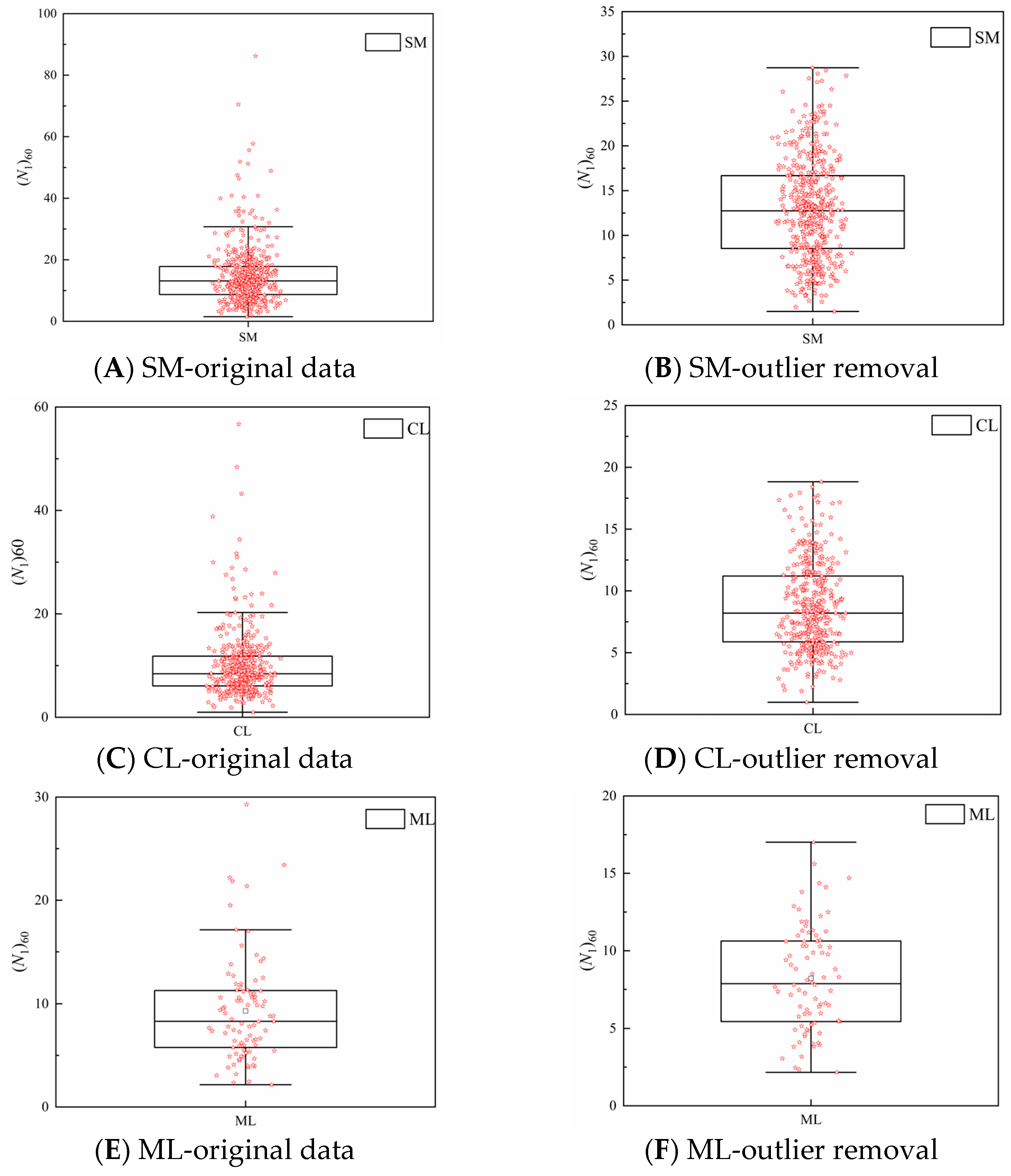
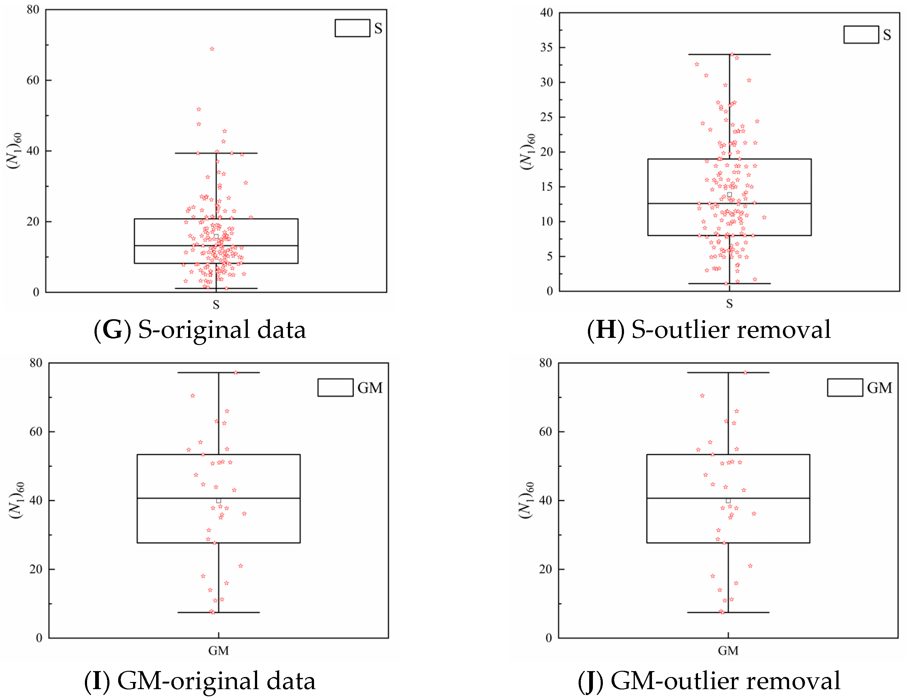
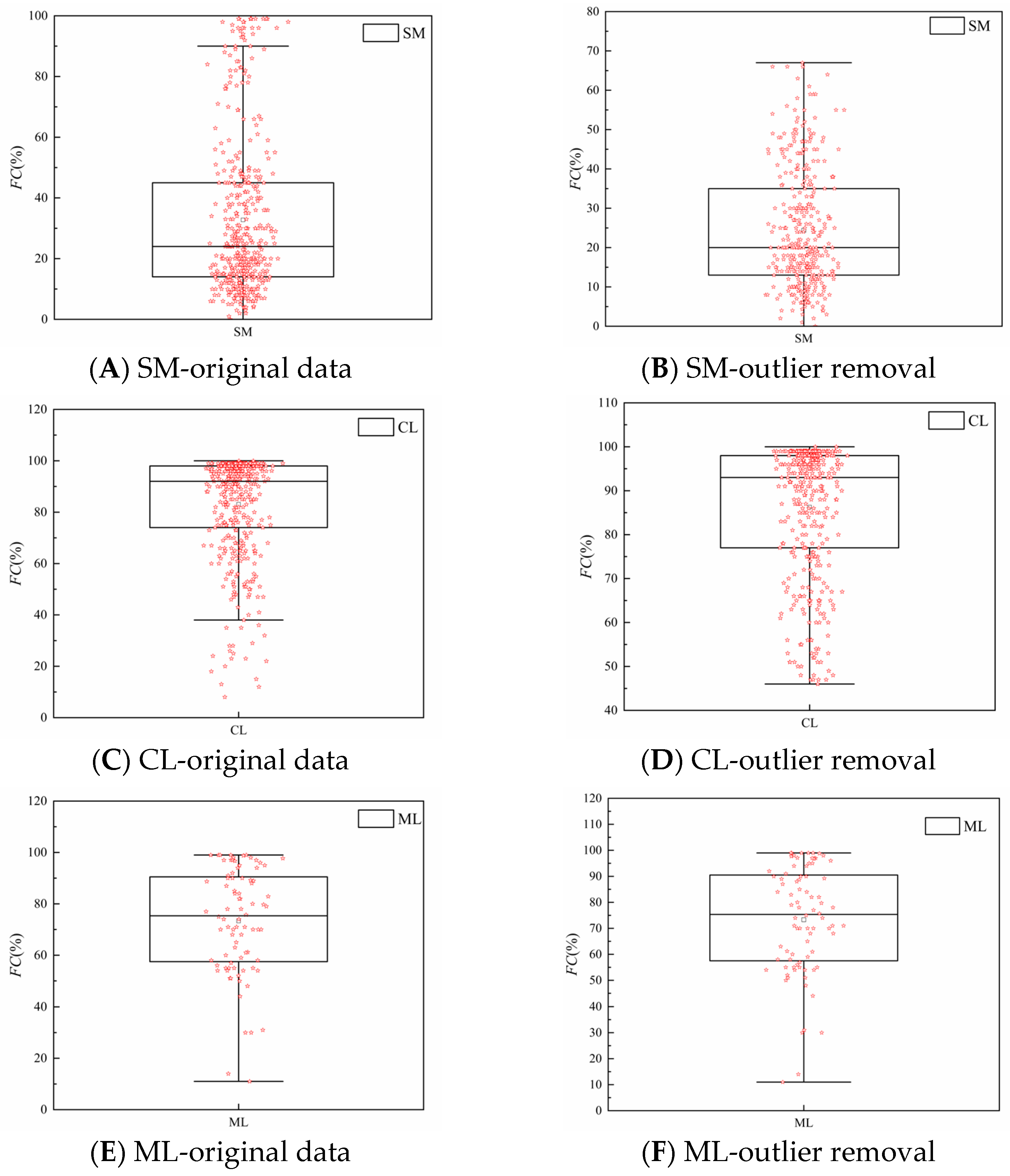
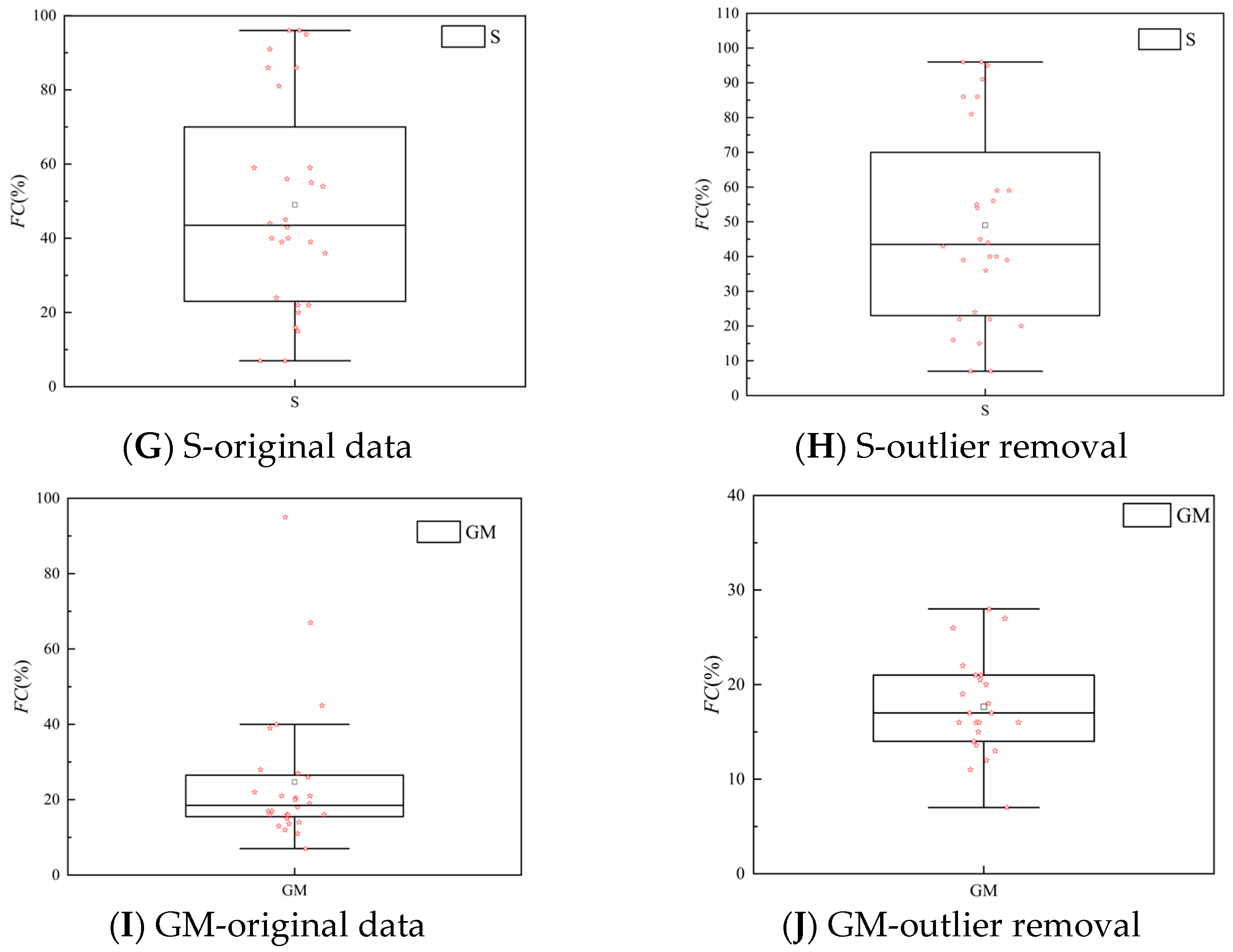
Figure 2, Figure 3 and Figure 4 illustrate the samples’ data distribution before and after the cleaning of data outliers. The data after cleaning were more concentrated, showing that there were more sample points near the mean value on the whole. On both sides, the points gradually decreased, and some of the sample variables tended to be concentrated around the deviation from the mean. It can be deduced that the processed sample data roughly obeyed the probability distribution with a kurtosis, such as a Gaussian distribution or a lognormal distribution.

3. Study on the Soil Property Variables’ Probability Distribution

In the process of determining probability distributions, we first attempted to determine the distribution fitting using unprocessed (raw) data. It was found that the presence of outliers made it difficult to establish valid probability distributions. Specifically, outliers tended to stretch the tails of common distributions (such as normal or lognormal, etc.). The estimated parameters may deviate from the central tendency of the dataset or even lead to a fitting failure. Consequently, liquefaction probability calculations could not be performed. The distribution shape returned to a reasonable form by removing the data points that were obviously distant from the main data region. It was characterized by a concentration of samples within a central region and a gradual thinning toward both ends, exhibiting a trend consistent with the expected statistical characteristics of the corresponding soil type.
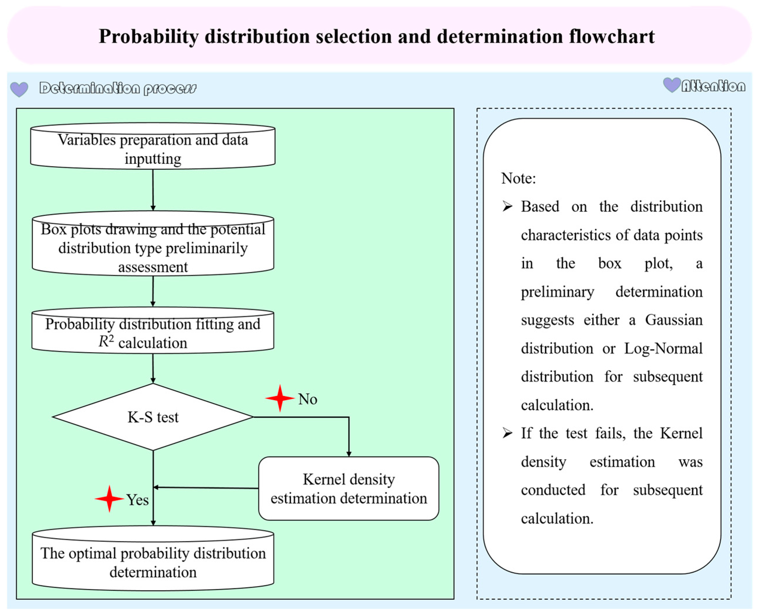
The soil factors (N1)60, FC, and d50 are continuous variables, and their probability distributions might follow a Gaussian or lognormal distribution according to the data characteristics [47,48,49]. Additionally, these two distributions pertain to the large numbers law as their theoretical basis and are the most commonly used distribution types in nature. Accordingly, the initial assumption is that the distribution types are a Gaussian distribution and a lognormal distribution based on the sample data characteristics in the box plot. The measured data were divided into intervals, the probability distribution fitting was conducted, and the determination coefficient R2 was calculated. A hypothesis test was then employed. If the hypothesis test passed and the R2 was relatively appreciable, it was determined that the factor follows the assumed distribution. If it failed to pass the hypothesis test, the kernel density estimation method was used to determine the probability density function. The above process is repeated in cycles until the probability distribution is determined [50,51,52]. The calculations for determining the probability distribution in this paper were implemented in PyCharm 2024, and the programming language was Python 3.12.2. The calculation flowchart is shown in Figure 5.

3.1. Interval Discretization and Probability Distribution Fitting

The determination of the probability distribution is influenced by the number of discretization intervals. If the number of intervals is too large, the distribution may become uniform, making it difficult to capture the true distribution characteristics. Conversely, if the number of intervals is too small, the fitting results may fail to accurately represent the overall distribution features [53,54]. The number of intervals was calculated using Equation (1), where N is the sample size and M is the number of intervals. Assuming the intervals’ lower and upper bounds were a and b, the average interval width was obtained from Equation (2). The histogram was fitted to both Gaussian and lognormal distributions, and the model performance was evaluated using the determination coefficient R2, where values closer to one indicate a better fit and accuracy. The Levenberg–Marquardt iterative optimization algorithm was adopted for distribution fitting. The advantages of gradient descent and the Gauss–Newton method were combined, which was appropriate for solving the least squares problem. By minimizing the squared sum of the distribution fitting errors, the fitting accuracy and stability were improved. The detailed process referred to the research of [53] and Ding et al. [54].
M = 1 + 3.3 × L o g N
Δ = b a M

3.2. Probability Distribution Hypothesis Test

It is important to consider not only the model’s R2 but also the results of hypothesis testing when finally determining the probability distribution. A high R2 indicates a better fit, offering accurate sample explanations, while hypothesis testing ensures it aligns with the data. Therefore, hypothesis testing was combined with R2 for the evaluation. The factors passing the hypothesis test and with a high R2 were considered to follow a specific distribution [53].
Common probability distribution hypothesis tests include the chi-square test, Kolmogorov–Smirnov test (K-S test), and Anderson–Darling test (A-D test) [53]. Among these, the K-S test is widely used to evaluate the fitting performance between the sample distribution and theoretical distribution. The maximum difference between the sample and the theoretical distribution is calculated based on the cumulative distribution function (CDF) F(x) to determine whether the sample originates from the specified distribution. It is particularly effective for continuous variables and performs well in small-sample scenarios. Considering that the soil factors were continuous and some samples were limited, the K-S test was an appropriate hypothesis testing approach for this research study. The testing procedure was as follows:
Step 1: Assuming that the sample came from the specified distribution, it was sorted from smallest to the largest, denoted as X1, X2, and Xn, and the empirical CDF Fn(x) is calculated as follows:
F n x = i = 1 k X i x n
Step 2: The K-S statistic Dn, defined as the maximum deviation between the sample and theoretical distributions, was calculated and compared with the critical value at the 95% confidence level, and then the p-value was obtained. If Dn was less than or equal to the critical value, the null hypothesis was accepted, indicating that it was consistent with the theoretical distribution.
D n = m a x F n x F x

3.3. Further Analysis of Factors Whose Probability Distribution Failed the Hypothesis Test

For soil type variables that did not conform to the above probability distribution, the kernel density estimation method was adopted in this paper to obtain the probability density function of the variables [54]. It is a non-parametric probability density function estimation method, which can make a reasonable estimate of the distribution form of the variable with limited observed samples, and is usually applicable to situations in which the variable distribution is unknown. Its core idea is to construct a smooth density curve by superimposing the “kernel function” (such as Gaussian kernel) around each data point. The kernel function estimates the probability density locally around each observation, and the global density is formed by aggregating these estimates. The calculation steps were as follows:
Step 1: Preparing the data, denoted as Y1, Y2, and Yn, the kernel density estimation function is as follows:
f h y = 1 n i = 1 n K h y Y i = 1 n h i = 1 n K y Y i h
where Kh(yYi) is the kernel function; n is the number of samples; and h is the bandwidth, which is used to control the smoothing.
Step 2: Determining the kernel function, for which the Gaussian kernel was selected to calculate the density function, and u was the standardized distance:
K u = 1 2 π e 1 2 u 2
Step 3: Determining the optimal bandwidth, which can be calculated by Equation (7), and inputting it into Equation (5) to obtain the density function, where σ is the standard deviation:
h = 1.06 σ n 1 5

4. Probability Distribution Determination Results

4.1. Probability Distribution Fitting

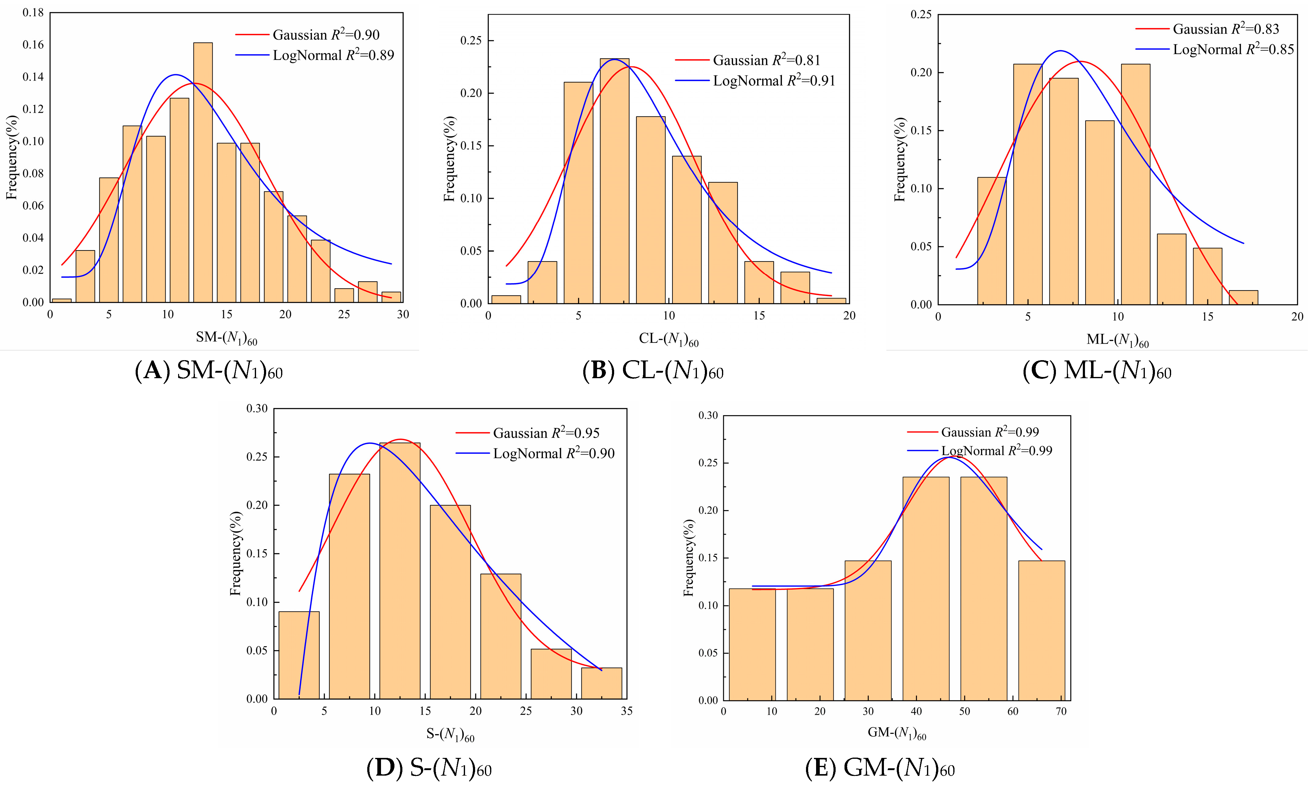
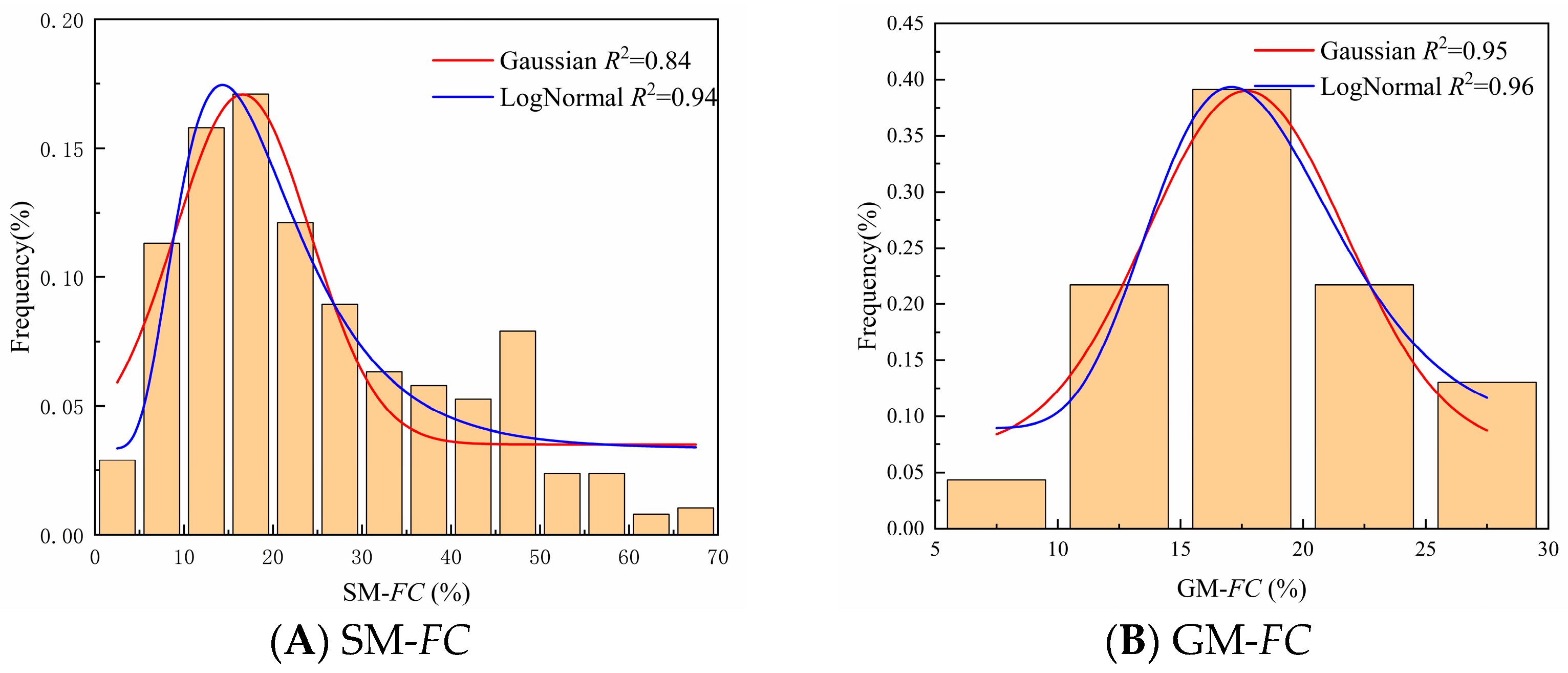
The probability distributions of soil factors (N1)60, FC, and d50 for different soil types were fitted, and the R2 was calculated based on the fitting results. The probability distributions with better fitting are summarized in Figure 6, Figure 7 and Figure 8.
The fitting performance is illustrated in Figure 6, Figure 7 and Figure 8. For (N1)60 under different soil type conditions, the best fitting performances of the Gaussian distribution were SM and S, while the best performances of the lognormal distribution were CL and ML. The fitting results were comparable to the two distributions for GM. For FC under different soil type conditions, the best fitting performances of the Gaussian distribution were SM and GM, while the fit for the other three soil types was poor for both the Gaussian and lognormal distributions, which required further study. For d50 under different soil type conditions, the best fitting performances of the lognormal distribution were SM, CL, and S, while the fitting for ML was the lognormal distribution. GM did not conform to either of these two distributions and required further study.

4.2. Probability Distribution Hypothesis Testing Results

As stated in the previous section, some of the factors under different soil types have better fitting. Hypothesis tests for these factors were conducted to further determine the distribution of each factor. Table 3 presents the hypothesis testing results of the soil factors.
The maximum p-values of the Gaussian distribution for (N1)60 under SM, S, and GM were 0.31, 0.25, and 0.80, respectively, while the R2 was also optimal. It demonstrated that (N1)60 under SM, S, and GM followed a Gaussian distribution. The maximum p-value of the lognormal distribution for (N1)60 under CL and ML were 0.69 and 0.76, respectively, while the R2 was also optimal. At the same time, it demonstrated that (N1)60 under CL and ML followed a Gaussian distribution. The maximum p-values of the lognormal distribution for FC under SM and GM were 0.28 and 0.88, respectively, while the R2 was also optimal. At the same time, it demonstrated that FC under SM and GM followed a lognormal distribution. The maximum p-value of the Gaussian distribution for d50 under ML was 0.23 and the Gaussian distribution for d50 under S was 0.53, while the R2 was also optimal. At the same time, it demonstrated that d50 under ML and S followed the Gaussian and lognormal distributions, respectively. However, SM and CL failed to pass the hypothesis test, which indicated that they did not conform to these two distributions and required further analysis.

4.3. Further Analysis of the Factors That Failed the Hypothesis Test

According to the previous section, FC under CL, ML, and S did not follow the above Gaussian and lognormal distributions, while d50 under SM, CL, and GM also did not follow the distributions. It did not follow the conventional distribution, as shown by the frequency distribution histograms of these factors. In this paper, the kernel density estimation method was adopted to estimate the probability density. The calculation results are shown in Figure 9.
Figure 9 shows multi-peak shapes with different forms for the frequency distribution histograms of these variables, while the curves obtained by the kernel density estimation method can be accurately fitted to the distribution shapes for each factor. The fitting results were good.

5. Liquefaction Probability Calculation Given the Distribution of Influencing Factors

5.1. Method for Determining Liquefaction Probability Based on Variable Distributions

Based on the established field liquefaction investigation case database, the empirical probability distributions of (N1)60, FC, and d50 under different soil types were systematically investigated in this study. Furthermore, the occurrence of liquefaction depends not only on soil properties but also on dynamic loading and environmental conditions [1]. Dynamic loading is the fundamental cause of liquefaction and can be characterized by two factors: magnitude (M) and peak acceleration (amax). The empirical probability distributions of M and amax can be derived from a probability seismic hazard analysis (PSHA) and the Gutenberg–Richter model [55]. The environmental conditions such as groundwater table (dw), burial depth (ds), total stress (σv), and effective stress (σv’) can also be determined using statistical methods similar to those employed in this study or by treating them as fixed values.
The interrelationship among these factors can be depicted by the joint distribution model, and the liquefaction probability can be further computed. The joint distribution considered environmental conditions, dynamic loading, and soil properties, which provided a scientific basis for quantitatively evaluating the liquefaction risk. The process is summarized as follows.
The limit state equation is a widely recognized method to evaluate the liquefaction probability, as illustrated in Equation (8). The CSR and CRR of soil can be characterized by M, amax, (N1)60, FC, d50, ds, dw, σv, and σv0′, and the calculation of CSR and CRR was performed according to the Seed method [1]. The liquefaction probability can be expressed as follows [1]:
g C S R , C R R = C R R C S R 0
P L = g N 1 60 , F C , d 50 , d s , d w , σ v , σ v , M , a m a x f N 1 60 , F C , d 50 , d s , d w , σ v , σ v , M , a m a x d N 1 60 d F C d d 50 d d s d d w d σ v d σ v d M d a m a x
It involves the joint distribution of multiple factors influencing liquefaction (f((N1)60, FC, d50, σv, σv’, ds, dw, M, and amax), as calculated in Equation (9), which is considerably complex and cannot provide an explicit solution. Consequently, simplified calculations are required. If the various factors are independent to each other, the complex joint distribution can be directly obtained by the product of the marginal distributions. In general, M and amax are not correlated with (N1)60, FC, d50, σv, σv’, ds, or dw, but soil factors (N1)60, FC, and d50. Environmental conditions σv, σv’, ds, and dw may not be completely independent. The joint distribution simplified calculation cannot be directly performed and cannot be simply decomposed into the product of the marginal distribution, which indicated that further analysis is required.
Traditional methods, such as the Youd method (proposed by Youd et al. [9]), Idriss method (proposed by Idriss and Boulanger [37]), and Cetin method [8], treat each factor as a deterministic value during calculations, thereby neglecting the inherent uncertainties in and statistical correlations among variables [8,9,10]. This simplification limits their ability to meet the precision and structural demands of real-world engineering. Generally, multivariate joint distribution modeling typically faces two major challenges: insufficient data to derive the joint probability density function; and the existence of inter-variable correlations that preclude independent modeling, limiting the application. In contrast, the Monte Carlo simulation method circumvents the explicit joint distribution function. By utilizing the marginal distributions of individual variables along with a correlation matrix, it is possible to generate samples that preserve the actual inter-variable dependence structure. It effectively avoids the difficulties associated with high-dimensional integration and complex function modeling. Therefore, Monte Carlo simulations for calculating the liquefaction probability using the probability distribution of known factors were proposed in this paper. The detailed computations and procedures are presented in the following section [55].

5.2. The Principle and Process of Liquefaction Probability Calculations Using Monte Carlo Method

The probability distributions of various soil property variables are presented in Section 4. Based on these distributions, the Monte Carlo method for calculating the liquefaction probability was proposed. The correlation coefficient metrics among variables was determined first. The Monte Carlo simulation was combined with the Cholesky decomposition technique to generate random samples of the variables that preserve the specified correlation structure. Each generated sample was then substituted into Equation (8) or (9) to assess whether liquefaction occurs. By generating a large number of samples, it can statistically simulate the liquefaction probability under specific conditions, thereby enabling assessments of the likelihood of soil liquefaction. The detailed procedure was as follows:
  • Step 1: Determination of correlations among the variables in the joint distribution
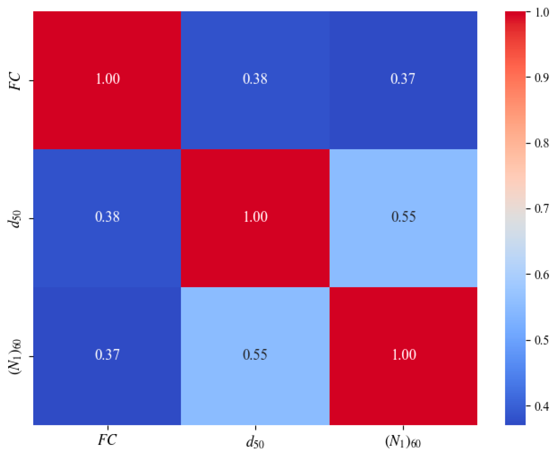
As demonstrated in Section 5.1, M and amax are not correlated with (N1)60, FC, d50, ds, dw, σv, or σv’, but (N1)60, FC, d50, ds, dw, σv, and σv’ may not be completely independent. Given that the probabilistic distributions of the environmental factors ds, dw, σv, and σv’ were not investigated in this study, these variables were temporarily treated as deterministic values for both this section and the subsequent case verification. The joint distribution of M and amax can be determined using the probabilistic seismic hazard analysis method. Therefore, only the inter-variable correlations among (N1)60, FC, and d50 need to be further considered. The correlation coefficient was calculated by Equation (10), and the correlation coefficient heat maps of (N1)60, FC, and d50 are illustrated in Figure 10.
r = X i X Y i Y X i X 2 Y i Y 2
where Xi and Yi are the data points of the two variables; X , Y are, respectively, the mean values of the variables; and r is the correlation coefficient.
  • Step 2: Sample generation with a certain correlation using the Monte Carlo method
The Monte Carlo random sampling method was adopted to generate samples that conform to a specific probability distribution to calculate the liquefaction probability through repetitive random sampling processes [29]. The operational steps using a Monte Carlo simulation to generate the samples confirming the distribution usually include the generation of uniformly distributed random numbers by pseudo-random number generators (PRNGS) in computers. These random numbers are uniformly distributed within the range of [0, 1). Through mathematical transformation, it finally can be converted into the target distribution samples [55].
The correlation coefficient matrix was obtained after correlation coefficient calculations. The Monte Carlo simulation method was used to generate independent samples that conform to the distribution types. The generated samples were adjusted according to the correlation coefficient matrix to make them conform to the correlations among the influencing factors through the Cholesky decomposition method. The Cholesky decomposition method transformed independent samples through a positive definite matrix (i.e., the correlation coefficient matrix) to achieve the expected correlation relationship. The samples were substituted into the limit state equation, and the number of samples that meet the liquefaction conditions were counted, thereby obtaining the liquefaction probability. The principle of Cholesky decomposition references the research of [55].
  • Step 3: Liquefaction probability calculation with the generated samples
Sampling was conducted within the interval near the measured sample points in this paper by setting a reasonable sampling interval. The sampling interval was set to the different standard deviation ranges that are generally adopted in interval sampling. The probability distribution form and parameters of (N1)60 referred to the research of [53].
The g((N1)60, FC, d50, σv, σv’, ds, dw, M, amax) of each sample was calculated after obtaining the samples, and the number of samples with g((N1)60, FC, d50, σv, σv’, ds, dw, M, amax) < 0 were counted. The liquefaction probability can be estimated by the following Equation (11).
P L t h e   samples   satisfied   g 0 t o t a l   samples

5.3. Case Verification Clculation

In order to further evaluate the effectiveness of the proposed Monte Carlo-based method for liquefaction probability calculations using variable probability distributions, a real-world engineering case from the 1975 Haicheng earthquake was selected for validation in this paper.
The sample was independent from the dataset, with (N1)60 = 7.6, and FC = 50%, d50 = 0.06 mm, M = 7, amax = 0.2 g, ds = 8.2 m, dw = 1.5 m, σv = 155 Kpa, and σv0′ = 89 Kpa. The sample was actually located near the Panjin Fertilizer Plant and the soil type is ML. During this earthquake, Sand boiling occurred near the samples. It was taken as a real-world example to verify the effectiveness of the proposed methods [8,9,10].
The distribution of (N1)6 was a lognormal distribution for ML, d50 under ML was a Gaussian distribution, and the FC under ML was calculated by the kernel density estimation. The calculation’s aim is to generate influencing factor samples under a given distribution by using a Monte Carlo simulation. According to the previous section, the samples following a specific distribution were finally generated.
To simplify calculations, dynamic loading M and amax as well as environmental conditions σv, σv’, ds, and dw were temporarily regarded as constant values in this paper. A total of 1000 samples within different standard deviation intervals were generated. The value of the standard deviation for ML was calculated and is summarized in Table 1. The generated samples were substituted into Equation (8) to determine whether they undergo liquefaction. Counting the number of samples that liquefied and substituting it into Equation (11), we can calculate the liquefaction probability.
The Youd method, the Idriss method, and the Cetin model were selected as comparison methods to evaluate the effectiveness of the method proposed in this paper. These methods are widely employed in soil liquefaction assessments, and the calculation principles and parameter determination procedures followed the studies of Youd, Idriss, and Cetin, respectively.
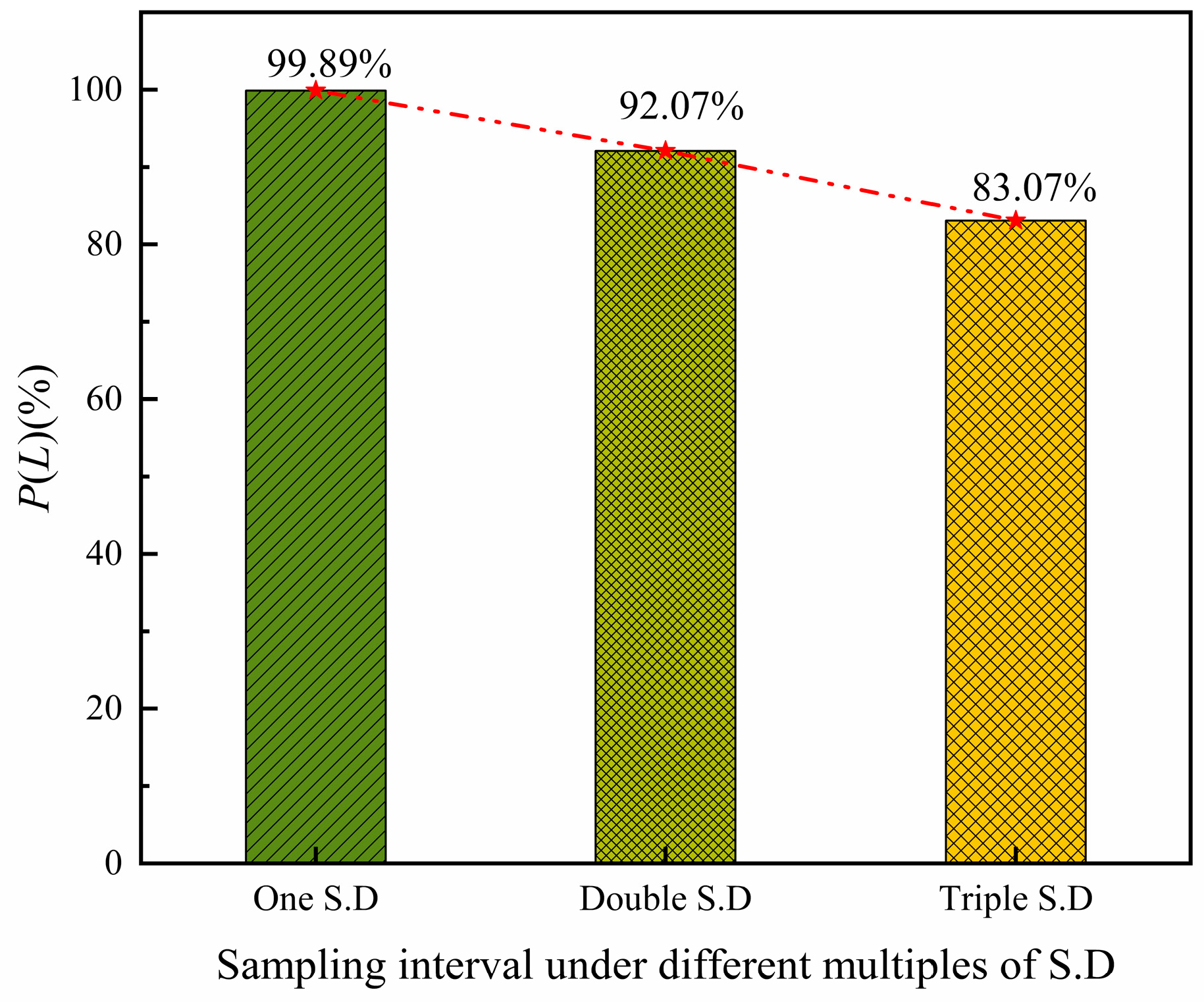
Figure 11 presents the result for the method under varying standard deviations. The liquefaction probabilities for one, two, and three standard deviations were 99.89%, 92.07%, and 83.07%, respectively. It can be concluded that liquefaction is highly likely to happen in this scenario, which is consistent with real-world conditions. The effectiveness of the method was validated. As the range increased from one to three standard deviations, the liquefaction probability decreased, and there was an obvious impact of sampling intervals on the probability calculation. Larger standard deviations widen the sampling range, and the generated samples were further from the measured values. Therefore, sampling should be conducted within smaller standard deviation ranges to better align with actual conditions.
Additionally, the measured values of each factor for this case were substituted into the Youd, Idriss, and Cetin models, and the liquefaction probabilities were obtained as 84.23%, 90.06%, and 99.84%, respectively. The probability was 99.89% when calculated by the proposed method, which was considerable to that obtained via the previous Youd, Idriss, and Cetin models. The calculation results confirmed that liquefaction would occur in this case, which was consistent with the actual observations, the effectiveness of the method was validated.

5.4. Sensitivity Analysis

The error standard deviation was considered when sampling according to the method, and the control variable method was adopted to analyze the influencing factor sensitivity on the results. In this section, one factor was fixed, respectively, and regarded as a constant value; only the other factors were sampled. The proposed methods were then used to calculate the liquefaction probability.
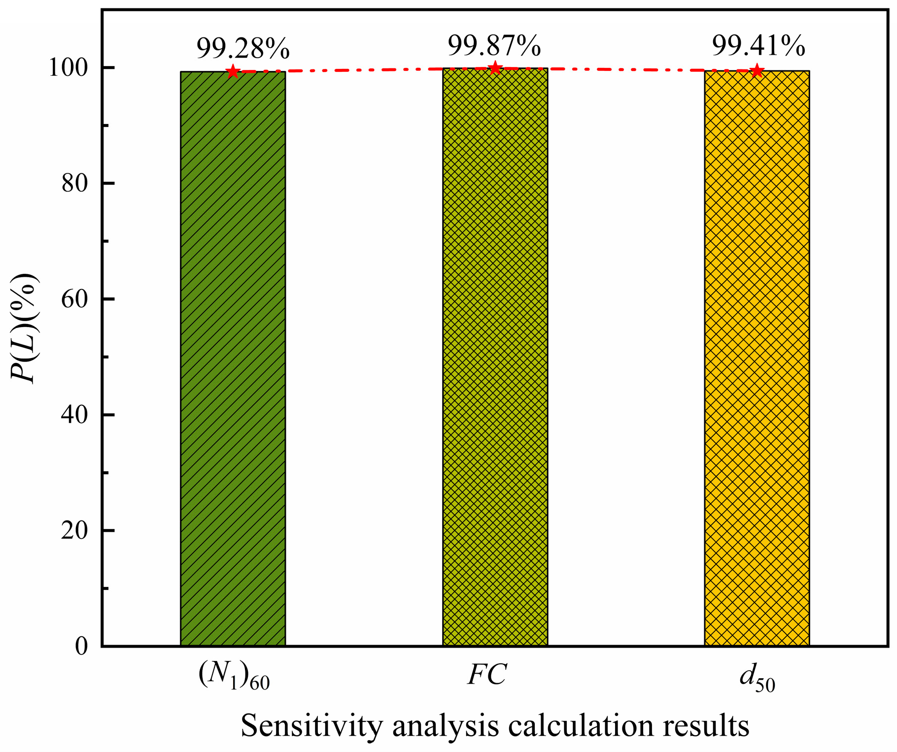
Figure 12 presented the sensitivity analysis calculation results under one standard deviation. When keeping (N1)60, FC, and d50 unchanged, respectively, there was little influence on the probability, and the P(L) values were 99.28%, 99.87%, and 99.41%, respectively. While sampling each factor simultaneously, the P(L) was 99.89%, and the difference was within 1.00%. It was indicated that the sensitivity was relatively low, varying with other various factors as part of the used method, and the computational stability was relatively robust.

6. Discussion

The collected samples in this study came from diverse regions, with varying soil types and geological conditions, which introduced uncertainty in the environmental factors’ probability distribution. These differences could affect the calculation accuracy if it was not accounted for. To reasonably quantify the modeling uncertainty caused by regional differences, normally distributed error terms were introduced in this paper, following the approach proposed by Gao [53], to incorporate the influence of regional soil characteristics into the probabilistic analysis framework. The normal distribution is mathematically symmetric, with its probability density function centered around the mean, making it suitable for representing unbiased uncertainty. Due to its simplicity and analytical tractability, it is widely used in engineering applications. Existing studies have shown that, in the absence of systematic regional bias, introducing normally distributed error terms provides a simple and effective way to account for spatial variability.
The principles and rationale for determining the mean and standard deviation of the normally distributed error term were as follows. In the absence of evidence indicating a systematic overestimation or underestimation in a specific region, setting the mean of the error term to zero ensures that the deviations are symmetrically distributed, avoiding any artificial bias [53]. An error term with a mean of zero only altered the variance structure of the model output without affecting its expected value. In this way, the error term serves as a perturbation, reflecting the degree of regional variability, rather than functioning as a correction factor. Therefore, the mean value of the error term was set to zero in this paper, indicating that there was no systematic deviation.
The standard deviation (σ) is the most critical parameter in the normally distributed error term, as it reflects the intensity of regional variability and directly influences the confidence level of the model in different regions. To enable the error term to be sensitive to regional characteristics, a standard deviation construction method was employed based on the deviation of regional sample means, following the method of Gao [53]. The detailed process is outlined in the following paragraph.
The global mean value (μglobal) of the certainty factor was first calculated using the population of samples across the dataset. For the i-th region, μregion,i represented the regional mean, and Δi = |μglobalμregion,i| was defined as the absolute deviation between μglobal and μregion,i. Then, the standard deviation of the error term for the i-th region was defined as σi = kΔi, where k was a tunable scaling coefficient (set to one in this paper) to control the overall intensity of the perturbation.
A larger deviation of the regional mean from the global mean indicated that the region exhibits more distinct environmental characteristics. Consequently, a stronger perturbation was introduced into the model to better represent regional heterogeneity. It did not rely on subjective assumptions or external priors; instead, it was derived directly from sample-based statistical characteristics, ensuring a degree of objectivity and reproducibility.
It is sensitive to regional differences and offers greater stability than conventional variance estimation methods, which may be heavily influenced by sample size fluctuations. It is based solely on the difference in means, which is particularly suitable for cases in which the sample size per region is limited. The standard deviation constructed in this method was different from the conventional sample standard deviation or variance in a strict statistical sense, but rather a proxy indicator of relative regional deviation. While it may lack formal statistical rigor, it offers a high degree of interpretability and practical feasibility, making it a fast and effective approach under conditions of sparse regional data.
Specifically, the case used in this paper came from China. The mean values of (N1)60, FC, and d50 in China were 10.30, 65.00%, and 0.055 mm, respectively, after the calculation, compared to those of the population of samples, which were 9.30, 72.50%, 0.045 mm, respectively. The absolute values of the mean differences for (N1)60, FC, and d50 were 1.00 m, 5.50%, and 0.01 mm, respectively. According to the error term construction method, the normal error terms of each factor follow the normal distribution (0,1.002), (0,5.502), and (0,0.012), respectively. The sampling results considering regional differences can be obtained by adding the error terms of each factor, respectively, to the sample generation processes under the method. Substituting it into the calculation processes, the liquefaction probability can be calculated, which is 99.93% (increased by 0.04%). It demonstrated the rationale of considering regional differences by using the normal distribution error term and that this method can improve the calculation accuracy to a certain extent.
It should be noted that, in order to simplify the calculation, amax, M, and other environmental factors were regarded as constant values, and the uncertainties were ignored in the case study. To actually determine the amax and M of the sample points, the PSHA method can be used to obtain the joint distribution P(amax, M) within a certain period of the site. The method proposed in this paper can either regard amax and M as fixed values to calculate the liquefaction probability at a specific seismic level, or combine the results of PSHA and substitute the joint distribution P(amax, M) to determine the total probability of possible liquefaction occurring within a certain period in the future. Whether the liquefaction probability is calculated for a specific seismic scenario using a single seismic event or at specific liquefaction probability level that may occur at the site in a certain period of time, both are aligned with the current engineering seismic analysis requirements. The calculated liquefaction probability can provide information for seismic design decisions, including site classification, liquefaction hazard zoning, and assessments of ground improvement requirements. In addition, it provides practical value for seismic hazard mapping and offers support for performance-based design in earthquake-prone areas. The method proposed in this paper can provide engineers with specific liquefaction probability calculations and can be used to guide the design of seismic infrastructure.
However, if the probability distribution of amax and M is considered in the method proposed in this paper in the future, the uncertainty would be inherited due to the PSHA calculation method. In addition, the samples of these environmental factors exist in different soil types and geological environments and are spread across multiple regions around the world. The influence of the above factors should be further considered for improving the proposed methods. The calculation method was only validated based on an actual case study from China, and it still needs to be validated in other regions around the world if it is to be promoted. Only after a large number of practical tests can it be used in engineering practice.

7. Conclusions

Based on the collected SPT field liquefaction investigation cases, descriptive statistics were conducted. Through probability distribution fitting, hypothesis testing, and kernel density estimations, the probability distribution curves of the soil factors (N1)60, FC, and d50 were determined. The liquefaction probability calculation method using Monte Carlo simulations was then proposed built on the influencing factors’ probability distribution. The effectiveness of these methods was validated through an actual case, and samples’ regional differences were considered by introducing the normal distribution error term. The conclusions are as follows:
(1)
The probability distributions of the same variable under different soil types were not identical. (N1)60, SM, S, and GM followed a Gaussian distribution, while CL and ML followed a lognormal distribution. FC, SM, and GM followed a lognormal distribution, while d50, ML, and S followed the Gaussian and lognormal distributions, respectively. The distribution curves of FC under CL, ML, S, and d50 under SM, CL, and GM can be calculated by the kernel density estimation;
(2)
The method of calculating liquefaction probability by using Monte Carlo simulations was feasible. The liquefaction probability calculation result of the case was similar to the existing probability model and consisted with the actual situation, indicating that the proposed methods are reliable;
(3)
Regional differences can be considered by introducing the normal distribution error term. The liquefaction probability accuracy can be improved to a certain extent. The method proposed in this paper can either regard amax and M as fixed values to calculate the liquefaction probability at a specific seismic level, or substitute the joint distribution P(amax, M) to determine the total probability within a certain period in the future.
While the proposed method provides a framework to calculate the liquefaction probability for a distribution, it should be noted that we did not explicitly incorporate the spatial variability of soil properties into the calculation. Given that soil is a heterogeneous granular material with significant spatial variation, future research should be paid to integrate spatial correlation structures or statistical methods to enhance the robustness and regional adaptability of the model. Additionally, due to limitations in the current dataset, only three representative soil parameters and five major soil types were selected to develop the respective distributions. The distribution parameters used may not fully capture the variability observed in broader geological contexts. As more data become available in the future, these distributions can be updated and refined to better reflect field conditions, thereby improving the precision of liquefaction probability estimations.

Author Contributions

Z.Y.: Writing—review and editing, Conceptualization, Supervision, Funding acquisition. M.F.: Writing—original draft, Writing—review and editing, Data curation, Formal analysis, Investigation, Methodology, Resources, Validation. J.L.: Supervision, Writing—review and editing. X.L.: Supervision, Writing—review and editing. J.Z.: Supervision, Writing—review and editing. H.Y.: Supervision, Writing—review and editing. All authors have read and agreed to the published version of the manuscript.

Funding

This work was supported by the National Key Research and Development Program of China (No. 2024YFF1700505, 2024YFF1700504); China Institute of Water Resource and Hydropower Research Basic Research Funds Special Project (No. GE0145B052021); and China Institute of Water Resource and Hydropower Research Sciences Scientific and Technological Achievements Transformation Fund (No. GE121003A0032022, GE121003A0032024).

Data Availability Statement

The data that support the findings of this study are available from the corresponding author upon reasonable request.

Conflicts of Interest

Author Hui Yang was employed by Yellow River Engineering Consulting Co., Ltd. The remaining authors declare that the research was conducted in the absence of any commercial or financial relationships that could be construed as a potential conflict of interest.

References

  1. Seed, H.B.; Idriss, I.M. Analysis of Soil Liquefaction: Niigata Earthquake. J. Soil Mech. Found. Div. 1967, 93, 83–108. [Google Scholar] [CrossRef]
  2. Kramer, S.L.; Seed, H.B. Initiation of Soil Liquefaction Under Static Loading Conditions. J. Geotech. Geoenviron. Eng. 1988, 114, 412–430. [Google Scholar] [CrossRef]
  3. Seed, H.B.; Idriss, I.M. Simplified Procedure for Evaluating Soil Liquefaction Potential. J. Soil Mech. Found. Div. 1971, 97, 1249–1273. [Google Scholar] [CrossRef]
  4. Fiegel, G.L.; Kutter, B.L. Liquefaction Mechanism for Layered Soils. J. Geotech. Geoenviron. Eng. 1994, 120, 737–755. [Google Scholar] [CrossRef]
  5. Wang, J.P.; Teng, C.C.; Sung, C.Y.; Xu, Y. Weighing the Influence of Geological and Geotechnical Factors in Soil Liquefaction Assessments. Nat. Hazards Rev. 2024, 25, 04024030. [Google Scholar] [CrossRef]
  6. Özener, P.T.; Özaydin, K.; Berilgen, M. Numerical and Physical Modeling of Liquefaction Mechanisms in Layered Sands. In Geotechnical Earthquake Engineering and Soil Dynamics IV; Proceedings; ASCE Library: Reston, VA, USA, 2012; pp. 1–12. [Google Scholar]
  7. Seed, H.B.; Idriss, I.M.; Arango, I. Evaluation of Liquefaction Potential Using Field Performance Data. J. Geotech. Geoenviron. Eng. 1983, 109, 458–482. [Google Scholar] [CrossRef]
  8. Cetin, K.O.; Seed, R.B.; Der Kiureghian, A.; Tokimatsu, K.; Harder Jr, L.F.; Kayen, R.E.; Moss, R.E. Standard Penetration Test-Based Probabilistic and Deterministic Assessment of Seismic Soil Liquefaction Potential. J. Geotech. Geoenviron. Eng. 2004, 130, 1314–1340. [Google Scholar] [CrossRef]
  9. Youd, T.L.; Idriss, I.M.; Andrus, R.D.; Arango, I.; Castro, G.; Christian, J.T.; Dobry, R.; Finn, W.D.L.; Harder Leslie, F.; Hynes Mary, E.; et al. Liquefaction Resistance of Soils: Summary Report from the 1996 NCEER and 1998 NCEER/NSF Workshops on Evaluation of Liquefaction Resistance of Soils. J. Geotech. Geoenviron. Eng. 2001, 127, 817–833. [Google Scholar] [CrossRef]
  10. Cetin, K.O.; Youd, T.L.; Seed, R.B.; Bray, J.D.; Stewart, J.P.; Durgunoglu, H.T.; Lettis, W.; Yilmaz, M.T. Liquefaction-Induced Lateral Spreading at Izmit Bay During the Kocaeli (Izmit)-Turkey Earthquake. J. Geotech. Geoenviron. Eng. 2004, 130, 1300–1313. [Google Scholar] [CrossRef]
  11. Cetin, K.O.; Seed, R.B.; Kayen, R.E.; Moss, R.E.S.; Bilge, H.T.; Ilgac, M.; Chowdhury, K. SPT-based probabilistic and deterministic assessment of seismic soil liquefaction triggering hazard. Soil Dyn. Earthq. Eng. 2018, 115, 698–709. [Google Scholar] [CrossRef]
  12. Han, X.; Gong, W.; Juang, C.H. Probabilistic evaluation of earthquake-induced liquefaction using Bayesian network based on a side-by-side SPT–CPT database. Can. Geotech. J. 2024, 61, 2653–2666. [Google Scholar] [CrossRef]
  13. Guan, Z.; Wang, Y. SPT-based probabilistic evaluation of soil liquefaction potential considering design life of civil infrastructures. Comput. Geotech. 2022, 148, 104807. [Google Scholar] [CrossRef]
  14. Acharya, I.P.; Subedi, M.; KC, R. Liquefaction Hazard Assessment of Kathmandu Valley Using Deterministic and Probabilistic Approaches. In Geo-Risk 2023; Proceedings; ASCE Library: Reston, VA, USA, 2023; pp. 307–317. [Google Scholar]
  15. Karagiannakis, G.; Di Sarno, L.; Necci, A.; Krausmann, E. Seismic risk assessment of supporting structures and process piping for accident prevention in chemical facilities. Int. J. Disaster Risk Reduct. 2022, 69, 102748. [Google Scholar] [CrossRef]
  16. Wu, Y.; Wang, J.; Cheng, J.; Yang, S. Dimension-Reduction Spectral Representation of Soil Spatial Variability and Its Application in the Efficient Reliability Analysis of Seismic Response in Tunnels. Reliab. Eng. Syst. Saf. 2024, 248, 110175. [Google Scholar] [CrossRef]
  17. Kameshwar, S.; Cox, D.T.; Barbosa, A.R.; Farokhnia, K.; Park, H.; Alam, M.S.; van de Lindt, J.W. Probabilistic decision-support framework for community resilience: Incorporating multi-hazards, infrastructure interdependencies, and resilience goals in a Bayesian network. Reliab. Eng. Syst. Saf. 2019, 191, 106568. [Google Scholar] [CrossRef]
  18. Jas, K.; Mangalathu, S.; Dodagoudar, G.R. Evaluation and analysis of liquefaction potential of gravelly soils using explainable probabilistic machine learning model. Comput. Geotech. 2024, 167, 106051. [Google Scholar] [CrossRef]
  19. Makdisi, A.J.; Kramer, S.L. Framework for Mapping Liquefaction Hazard–Targeted Design Ground Motions. J. Geotech. Geoenviron. Eng. 2024, 150, 04024123. [Google Scholar] [CrossRef]
  20. Guan, Z.; Wang, Y. Probabilistic Assessment of Soil Liquefaction Potential Using CPT-Based Smart Site Investigation Strategy. In Geo-Risk 2023; Proceedings; ASCE Library: Reston, VA, USA, 2023; pp. 145–154. [Google Scholar]
  21. Liao, S.S.C.; Veneziano, D.; Whitman, R.V. Regression Models For Evaluating Liquefaction Probability. J. Geotech. Geoenviron. Eng. 1988, 114, 389–411. [Google Scholar] [CrossRef]
  22. Yang, H.; Liu, Z.; Xie, Y. Probabilistic Liquefaction Assessment Based on an In-situ State Parameter Considering Soil Spatial Variability and Various Uncertainties. KSCE J. Civ. Eng. 2023, 27, 4228–4239. [Google Scholar] [CrossRef]
  23. Zhao, Z.; Duan, W.; Cai, G.; Wu, M.; Liu, S. CPT-based fully probabilistic seismic liquefaction potential assessment to reduce uncertainty: Integrating XGBoost algorithm with Bayesian theorem. Comput. Geotech. 2022, 149, 104868. [Google Scholar] [CrossRef]
  24. Hu, J.; Wang, J. Prediction of liquefaction of gravelly soils based on a cost-sensitive Bayesian network combined with rough set weighting. Gondwana Res. 2024, 131, 57–68. [Google Scholar] [CrossRef]
  25. Cruz, A.; Karimzadeh, S.; Chieffo, N.; Sandoval, E.; Lourenço, P.B. A Review of Probabilistic Approaches for Assessing the Liquefaction Hazard in Urban Areas. Arch. Comput. Methods Eng. 2024, 31, 4673–4708. [Google Scholar] [CrossRef]
  26. Sianko, I.; Ozdemir, Z.; Khoshkholghi, S.; Garcia, R.; Hajirasouliha, I.; Yazgan, U.; Pilakoutas, K. A practical probabilistic earthquake hazard analysis tool: Case study Marmara region. Bull. Earthq. Eng. 2020, 18, 2523–2555. [Google Scholar] [CrossRef]
  27. Wang, F.; Huang, H.; Yin, Z.; Huang, Q. Probabilistic characteristics analysis for the time-dependent deformation of clay soils due to spatial variability. Eur. J. Environ. Civ. Eng. 2021, 26, 6096–6114. [Google Scholar] [CrossRef]
  28. Lifshitz, S.G.; Urlainis, A.; Moyal, S.; Shohet, I.M. Seismic Resilience in Critical Infrastructures: A Power Station Preparedness Case Study. Appl. Sci. 2024, 14, 3835. [Google Scholar] [CrossRef]
  29. Huang, F.K.; Wang, G.S. A Method for Developing Seismic Hazard-Consistent Fragility Curves for Soil Liquefaction Using Monte Carlo Simulation. Appl. Sci. 2024, 14, 9482. [Google Scholar] [CrossRef]
  30. Wang, F.Y.; Zhai, W.Z.; Man, J.H.; Huang, H.W. A hybrid cohesive phase-field numerical method for the stability analysis of rock slopes with discontinuities. Can. Geotech. J. 2025, 62, 1–16. [Google Scholar] [CrossRef]
  31. Urlainis, A.; Ornai, D.; Levy, R.; Vilnay, O.; Shohet, I.M. Loss and damage assessment in critical infrastructures due to extreme events. Saf. Sci. 2022, 147, 105587. [Google Scholar] [CrossRef]
  32. Wang, Z.; Cudmani, R.; Pena, O.; Andres, A.; Zhang, C.; Zhou, P. Leveraging Bayesian methods for addressing multi-uncertainty in data-driven seismic liquefaction assessment. J. Rock Mech. Geotech. Eng. 2024, 17, 2474–2491. [Google Scholar] [CrossRef]
  33. Jain, A.; Oommen, T. Significance of Quantifying Uncertainties in Probabilistic Modeling and a Possible Approach to Select the Best: A Study Using SPT- and CPT-Based Liquefaction Case Histories. In Advances in Soil Dynamics and Foundation Engineering; Proceedings; ASCE Library: Reston, VA, USA, 2014; pp. 83–96. [Google Scholar]
  34. Tang, X.W.; Hu, J.L.; Qiu, J.N. Identifying significant influence factors of seismic soil liquefaction and analyzing their structural relationship. KSCE J. Civ. Eng. 2016, 20, 2655–2663. [Google Scholar] [CrossRef]
  35. Zhou, Y.; Wang, H.; Wu, W.; Sun, Y.; Huang, M.; Zhao, Z.; Zheng, Q. Quantitative study of the effects of loading conditions and physical parameters on the liquefaction properties of saturated sandy soils: A DEM and experimental investigation. Soil Dyn. Earthq. Eng. 2025, 190, 109187. [Google Scholar] [CrossRef]
  36. Klu, A.K.; Affam, M.; Ewusi, A.; Ziggah, Y.Y.; Boateng, E.K. Site classification and soil liquefaction evaluation based on shear wave velocity via HoliSurface approach. J. Afr. Earth Sci. 2025, 225, 105574. [Google Scholar] [CrossRef]
  37. Boulanger, R.W.; Idriss, I.M. Probabilistic Standard Penetration Test–Based Liquefaction–Triggering Procedure. J. Geotech. Geoenviron. Eng. 2012, 138, 1185–1195. [Google Scholar] [CrossRef]
  38. Gu, X.; Zuo, K.; Hu, C.; Hu, J. Liquefaction resistance and small strain stiffness of silty sand: Effects of host sand gradation and fines content. Eng. Geol. 2024, 335, 107546. [Google Scholar] [CrossRef]
  39. Yu, T.; Fleureau, J.M.; Souli, H.; Kong, X. The improved cyclic resistance of bio-treated sands with various gradations for liquefaction mitigation: Density increase and/or cementation? Soil Dyn. Earthq. Eng. 2024, 185, 108894. [Google Scholar] [CrossRef]
  40. El Ahmad, M.; Hubler, J. Investigating the Influence of Sand Particle Morphology on Post-Liquefaction Volumetric Strain of Two Uniform Sands. In Geo-Congress 2024; Proceedings; ASCE Library: Reston, VA, USA, 2024; pp. 415–424. [Google Scholar]
  41. Yang, S.; Huang, D. Understanding the influence of drained cyclic preloading on liquefaction resistance of sands using DEM-clump modeling. Comput. Geotech. 2024, 176, 106800. [Google Scholar] [CrossRef]
  42. Xu, M.Q.; Pan, K.; Duan, B.; Wu, Q.X.; Yang, Z.X. Investigating the influence of particle shape on discrete element modeling of granular soil under multidirectional cyclic shearing. Soil Dyn. Earthq. Eng. 2025, 189, 109097. [Google Scholar] [CrossRef]
  43. Molina, G.F.; Viana, F.A.; Ferreira, C.; Caicedo, B. Insights into the assessment and interpretation of earthquake-induced liquefaction in sands under different degrees of saturation. Earth-Sci. Rev. 2024, 258, 104925. [Google Scholar] [CrossRef]
  44. Upadhyaya, S.; Maurer, B.W.; Green, R.A.; Rodriguez-Marek, A.; van Ballegooy, S. Surficial liquefaction manifestation severity thresholds for profiles having high fines-content, high-plasticity soils. Can. Geotech. J. 2022, 60, 642–653. [Google Scholar] [CrossRef]
  45. Duan, W.; Congress, S.S.C.; Cai, G.; Zhao, Z.; Pu, S.; Liu, S.; Dong, X.; Wu, M.; Chen, R. Characterizing the in-situ state of sandy soils for liquefaction analysis using resistivity piezocone penetration test. Soil Dyn. Earthq. Eng. 2023, 164, 107529. [Google Scholar] [CrossRef]
  46. Jas, K.; Dodagoudar, G.R. Explainable machine learning model for liquefaction potential assessment of soils using XGBoost-SHAP. Soil Dyn. Earthq. Eng. 2023, 165, 107662. [Google Scholar] [CrossRef]
  47. Li, X.; Zhang, Y.; Yang, Z.; Qi, X. Estimation of site-specific multivariate probability distribution of soil properties using a mixed sampling technique. Comput. Geotech. 2024, 166, 105956. [Google Scholar] [CrossRef]
  48. Porwik, P.; Dadzie, B.M. Detection of data drift in a two-dimensional stream using the Kolmogorov-Smirnov test. Procedia Comput. Sci. 2022, 207, 168–175. [Google Scholar] [CrossRef]
  49. Harrop-Williams, K. Probability Distribution of Strength Parameters in Uniform Soils. J. Eng. Mech. 1986, 112, 345–350. [Google Scholar] [CrossRef]
  50. Chen, W.; Ding, J.; Shi, C.; Wang, T.; Connolly, D.P. Geotechnical correlation field-informed and data-driven prediction of spatially varying geotechnical properties. Comput. Geotech. 2024, 171, 106407. [Google Scholar] [CrossRef]
  51. Zhang, J.; Han, S.; Li, M.; Li, H.; Zhao, W.; Wang, J.; Liang, H. CasMDN: A deep learning-based multivariate distribution modelling approach and its application in geotechnical engineering. Comput. Geotech. 2024, 168, 106164. [Google Scholar] [CrossRef]
  52. Vanmarcke, E.H. Probabilistic Modeling of Soil Profiles. J. Geotech. Eng. Div. 1977, 103, 1227–1246. [Google Scholar] [CrossRef]
  53. Gao, D.Z. Reliability Principle of Soil Mechanics; China Architecture & Building Press: Beijing, China, 1989. [Google Scholar]
  54. Ding, J.H.; Liang, J.G.; Zhang, J.P.; Chang, W.J. Reliability Design Principle and Application of Foundation Engineering; China Water & Power Press, Intellectual Property Publishing House: Beijing, China, 2010. [Google Scholar]
  55. Zacchei, E.; Molina, J.L. Probabilistic Seismic Hazard Analysis for Andalusian Dams in Southern Spain Using New Seismogenic Zones. ASCE-ASME J. Risk Uncertain. Eng. Syst. Part A Civ. Eng. 2022, 8, 04022034. [Google Scholar] [CrossRef]
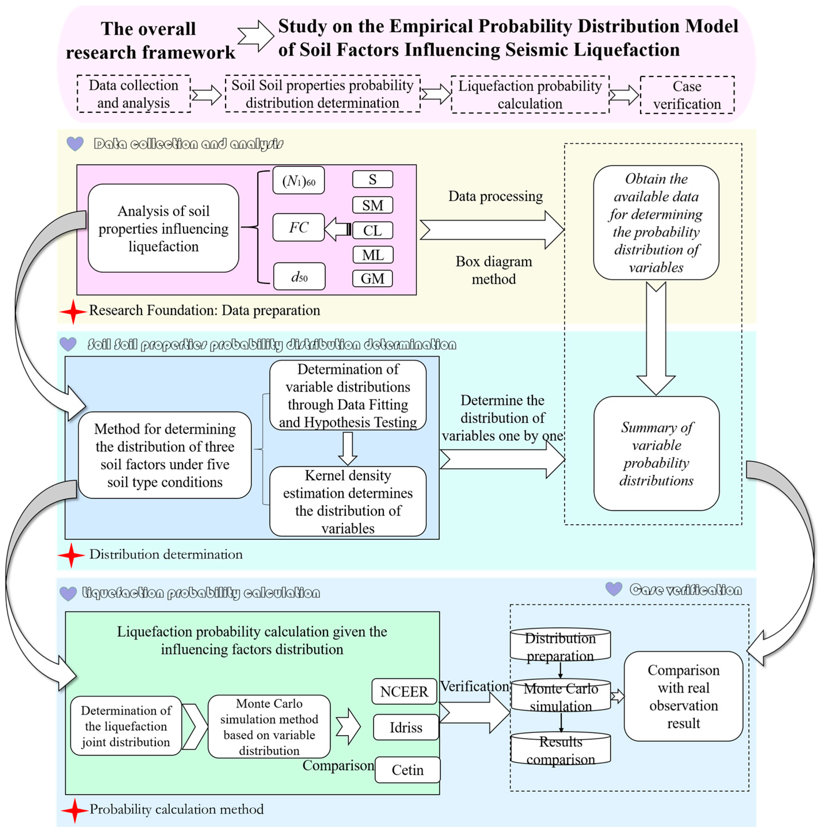
Figure 1. Overall research framework.
Buildings 15 02861 g001
Figure 2. (N1)60 box plot.
Buildings 15 02861 g002aBuildings 15 02861 g002b
Figure 3. FC box plot.
Buildings 15 02861 g003aBuildings 15 02861 g003b
Figure 4. d50 box plot.
Buildings 15 02861 g004aBuildings 15 02861 g004b
Figure 5. Probability distribution determination flowchart.
Buildings 15 02861 g005
Figure 6. (N1)60 probability distribution fitting under different soil type conditions.
Buildings 15 02861 g006
Figure 7. FC probability distribution fitting under different soil type conditions.
Buildings 15 02861 g007
Figure 8. d50 probability distribution fitting under different soil type conditions.
Buildings 15 02861 g008
Figure 9. Kernel density estimation results.
Buildings 15 02861 g009
Figure 10. Correlation coefficient heat map.
Buildings 15 02861 g010
Figure 11. Calculation results of the method under different standard deviation ranges.
Buildings 15 02861 g011
Figure 12. Sensitivity analysis calculation results.
Buildings 15 02861 g012
Table 1. Influencing factors considered in typical methods.
FactorsInfluencing Factors
MethodDynamic LoadingEnvironmental FactorsSoil Factors
Deterministic methodNCEERM, amaxds, dw, σ, σ(N1)60, FC, DR
Chinese codeM, amax, Rds, dwN, ρc
Probabilistic methodIdrissM, amaxds, dw, σ, σ(N1)60, FC, DR
Liaoamaxσ, σN
CetinM, amaxσ, σ(N1)60, FC
ChenM, amaxσ, σ(N1)60, FC, DR
Machine learning methodSupport vector machineM, ED, Rds, dwN
Neural networkM, amaxds, dw, σ, σ(N1)60, FC, d50
Bayesian networkM, amax, Rds, dw, σ, σ(N1)60, FC, d50, ST
Table 2. Descriptive statistics of soil properties.
Soil TypeFactorsMinimum ValueMaximum ValueMean ValueVarianceVariation
Coefficient
SM(N1)601.58614.7486.850.63
FC09932.75674.330.79
d500.0028960.5520.598.18
CL(N1)600.9856.689.9239.430.63
FC810083.07398.910.24
d500.00250.0430.065.74
ML(N1)602.1629.289.3025.630.54
FC5.739972.50477.350.30
d5000.220.0450.0010.80
S(N1)601.168.8715.78111.920.67
FC79649.22832.640.59
d500.0065150.574.083.54
GM(N1)607.4677.2039.94357.830.47
FC79524.72344.590.75
d500.0055122.9712.641.20
Table 3. p-value for hypothesis testing of fitted distributions (95% significance level).
Distribution
Name
GaussianLognormal
SMCLMLSGMSMCLMLSGM
(N1)600.310.020.510.250.800.000.690.760.180.13
FC0.000.000.000.000.760.280.000.000.000.88
d500.000.000.230.000.000.000.000.020.530.00
Disclaimer/Publisher’s Note: The statements, opinions and data contained in all publications are solely those of the individual author(s) and contributor(s) and not of MDPI and/or the editor(s). MDPI and/or the editor(s) disclaim responsibility for any injury to people or property resulting from any ideas, methods, instructions or products referred to in the content.