


AI-Powered Forecasting of Environmental Impacts and Construction Costs to Enhance Project Management in Highway Projects
Abstract
1. Introduction
- Section 1 presents the Introduction.
- Section 2 shows the database structure, including data collection, preprocessing, and feature selection strategies for both the planning and design phases.
- Section 3 details the development and configuration of ANN and DNN models, including architecture selection, hyperparameter optimization, and performance evaluation metrics.
- Section 4 compares the predictive performance of both model types, highlighting the trade-offs and suitability of each method for estimating EL and CC.
- Section 5 concludes the study by summarizing key findings, discussing limitations, and suggesting future research directions to improve machine learning applications in early-stage infrastructure planning.
2. Database Collection and Analysis
2.1. Collection of Road Project Cases
- Earthwork: quantities for operations such as excavation, earth moving, ripping, blasting rock, and ceramic transport (m3), including dump transport and green zone reclamation.
- Drainage: lengths of side ditches and horizontal drains (m), and volumes for structures such as VR halls, wing walls, and concrete placements (m3).
- Paving (Packer): volumes of frost protection layers (m3) and quantities of asphalt base, middle, and surface layers (tons).
- Structural labor: formwork areas (m3), rebar assembly (tons), and ladder work (tons), reflecting both material input and labor intensity.
2.2. Dataset Composition and Variable Selection for Model Development
2.2.1. Data Distribution, Missing Values, and Imputation Strategy in the Design-Stage Database
2.2.2. Handling Missing Values Through Imputation
| library(readxl) library(data.table) library(h2o) h2o.init() # Load and prepare dataset design_data <- as.data.table(read_excel(“design_db_.xlsx”)) h2o_data <- as.h2o(design_data) # Identify columns with missing values na_cols <- names(which(colSums(is.na(design_data)) > 0)) # Impute missing values using Random Forest for (col in na_cols) { model <- h2o.randomForest( x = setdiff(names(h2o_data), col), y = col, training_frame = h2o_data ) prediction <- as.data.frame(h2o.predict(model, h2o_data))$predict design_data[[col]][is.na(design_data[[col]])] <- prediction[is.na(design_data[[col]])] } # Resulting dataset imputed_design_data <- design_data |
2.2.3. Distribution Shift After Imputation
3. Artificial Neural Network
3.1. Selection of Optimal Variables
- Earthwork typically consists of 12 tasks, such as demolition, excavation, embankment formation, and topsoil removal.
- Slope safety involves vegetation-based and structural reinforcement.
- Drainage includes around 14 activities, such as trenching, blind hole drilling, and horizontal pipe installation.
- Paving work encompasses 13 procedures, including frost protection, compaction, concrete curing, and surface finishing.
- Traffic safety covers 11 elements like road signs and pavement markings.
- Ancillary works average 20 tasks and include features like protective walls, signage, and noise barriers.
3.1.1. Optimal Variable Selection Using Autoencoder
| # Define autoencoder depth (1 to 3 hidden layers) depth <- sample(1:3, 1) # Create 6-fold cross-validation indices folds <- createFolds(1:100, k = 6) # Hyperparameter search space hyperparams <- list( list( hidden = sample(100:500, depth, replace = TRUE), input_dr = sample(400:800, 1) / 1000, hidden_dr = sample(400:800, depth, replace = TRUE) ), list( hidden = sample(100:500, depth, replace = TRUE), input_dr = sample(400:800, 1) / 1000, hidden_dr = sample(400:800, depth, replace = TRUE) ), list( hidden = sample(100:500, depth, replace = TRUE), input_dr = sample(400:800, 1) / 1000, hidden_dr = sample(400:800, depth, replace = TRUE) ), list( hidden = sample(100:500, depth, replace = TRUE), input_dr = sample(400:800, 1) / 1000, hidden_dr = sample(400:800, depth, replace = TRUE) ), list( hidden = sample(100:500, depth, replace = TRUE), input_dr = sample(400:800, 1) / 1000, hidden_dr = sample(400:800, depth, replace = TRUE) ), list( hidden = sample(100:500, depth, replace = TRUE), input_dr = sample(400:800, 1) / 1000, hidden_dr = sample(400:800, depth, replace = TRUE) ) ) |
| Planning stage Autoencoder learning process coding details |
| fm_plan_Eco <- lapply(hyperparams, function(v) { lapply(folds, function(i) { h2o.deeplearning( x = 1:11, training_frame = train_plan_Eco[, −12], validation_frame = test_plan_Eco[, −12], distribution = “gaussian”, activation = “RectifierWithDropout”, hidden = v$hidden, rho = 0.90, epsilon = 1 × 10⁷, input_dropout_ratio = v$input_dr, hidden_dropout_ratios = v$hidden_dr, loss = “Automatic”, autoencoder = TRUE, sparse = TRUE, l1 = 1 × 10⁷, l2 = 1 × 10⁷, epochs = 300 ) }) }) |
| #Planning stage Autoencoder verification process coding details |
| fm.final_plan_Eco <- h2o.deeplearning( x = 1:11, training_frame = train_plan_Eco[, −12], validation_frame = test_plan_Eco[, −12], distribution = “gaussian”, activation = “RectifierWithDropout”, hidden = hyperparams[[5]]$hidden, rho = 0.90, epsilon = 1 × 10⁷, input_dropout_ratio = hyperparams[[5]]$input_dr, hidden_dropout_ratios = hyperparams[[5]]$hidden_dr, loss = “Automatic”, autoencoder = TRUE, l1 = 1 × 10⁷, l2 = 1 × 10⁷, epochs = 300 ) |
3.1.2. The Setting of Optimal Variables in the Design Phase
3.2. ANN
3.2.1. Construction and Preprocessing for Planning-Stage Estimation
| plan_Eco_ann <- h2o.deeplearning( x = 1:11, # Input features y = 12, # Target variable: EL training_frame = train_plan_Eco, validation_frame = valid_plan_Eco, nfolds = 2, distribution = “gaussian”, activation = “Rectifier”, hidden = sample(1:300, 1, TRUE), # Random neuron count in hidden layer rho = 0.90, epsilon = 1 × 10⁷, input_dropout_ratio = sample(400:800, 1, TRUE) / 1000, hidden_dropout_ratios = sample(400:800, 1, TRUE) / 1000, loss = “Automatic”, stopping_rounds = 5, stopping_metric = “AUTO”, stopping_tolerance = 0.01, sparse = TRUE, epochs = 300 ) |
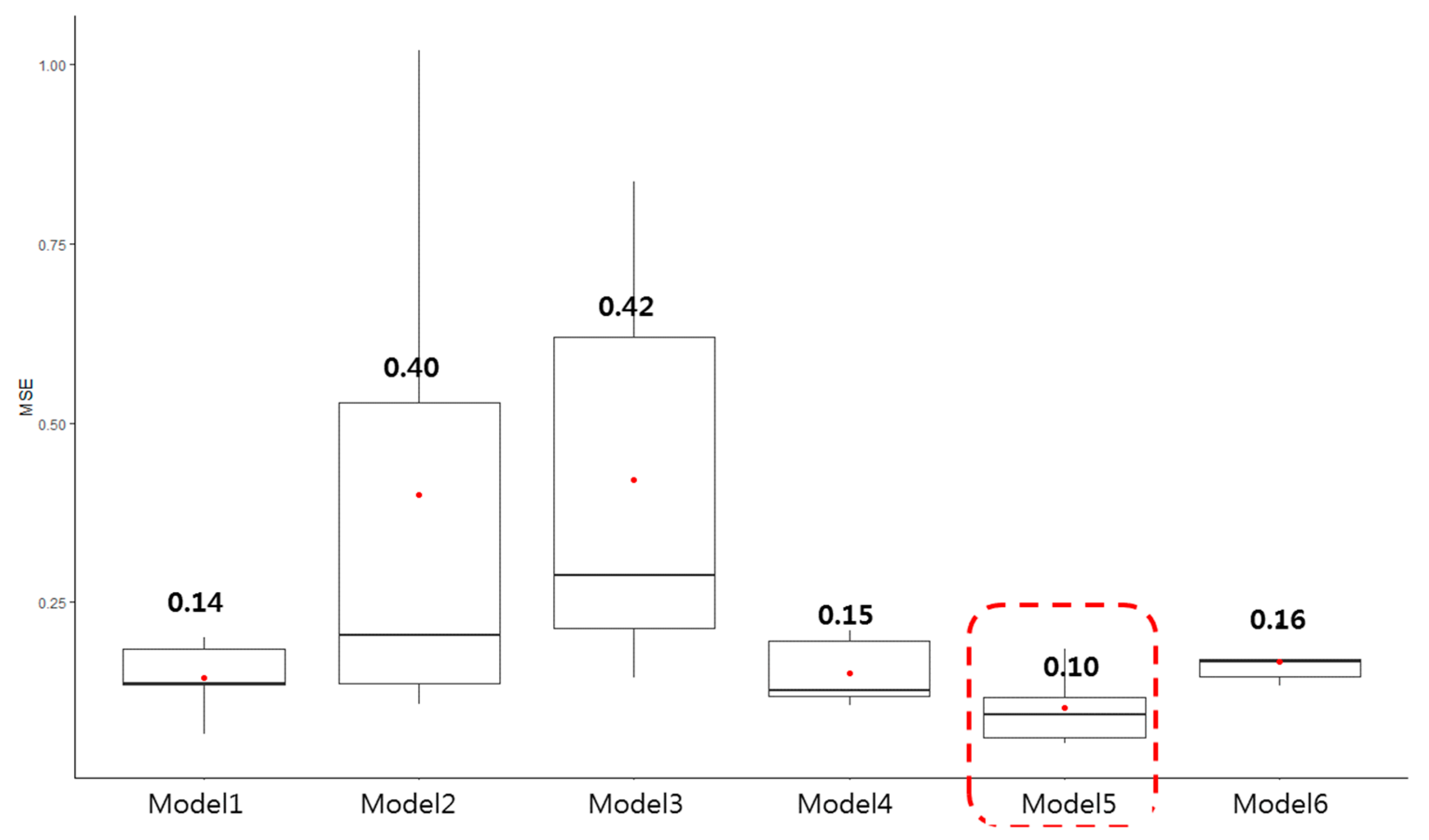
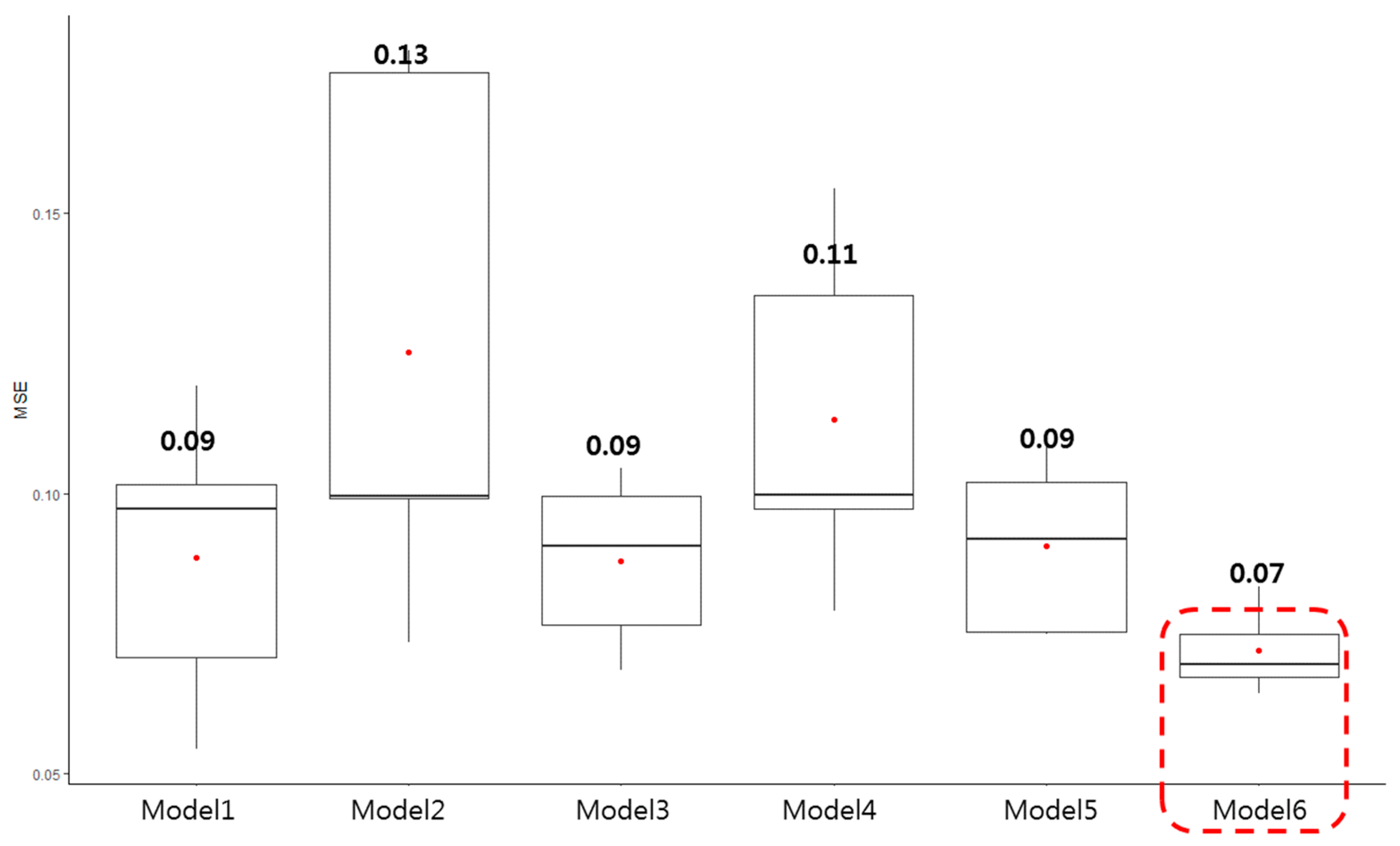
3.2.2. Prediction Accuracy and Optimal Architecture of ANN Models
3.3. Deep Neural Network
| # Building the DNN Model depth = sample(2:5, 1) # Randomly selecting depth (2 to 5 hidden layers) plan_Eco_dnn <- h2o.deeplearning( x = 1:11, # Columns 1 to 11 are the features y = 12, # Column 12 is the target variable (EL or CC) training_frame = train_dlan_Eco, validation_frame = test_dlan_Eco, nfolds = 2, # Number of folds for cross-validation distribution = “gaussian”, # Distribution type for the target variable activation = “Rectifier”, # Activation function hidden = sample(1:300, depth, TRUE), # Randomly select a number of hidden layers (up to 300 neurons) rho = 0.90, # Regularization parameter epsilon = 1e-07, # Convergence threshold input_dropout_ratio = sample(400:800, 1, TRUE) / 1000, # Input dropout ratio hidden_dropout_ratios = sample(400:800, depth, TRUE) / 1000, # Hidden layer dropout ratios loss = “Automatic”, # Loss function to use stopping_rounds = 5, # Stop training after 5 rounds of no improvement stopping_metric = “AUTO”, # Metric for stopping stopping_tolerance = 0.01, # Tolerance for stopping criteria sparse = TRUE, # Use sparse matrices epochs = 300 # Number of training epochs (can also use 500) ) # Prediction Process prediction_plan_Eco_dnn <- h2o.predict(plan_Eco_dnn, newdata = vali_plan_Eco) # Calculate the Error Rate error_rate <- mean(abs((prediction_plan_Eco_dnn$predict / vali_plan_Eco_1$Eco) − 1) * 100) # Print the error rate print(error_rate) |
3.3.1. Architecture and Prediction Performance for EL and CC Estimation
3.3.2. Optimal DNN Model Configuration and Performance Assessment
3.3.3. Additional Evaluation Metrics
4. Results
4.1. Comparison of ANN and DNN
4.2. Discussions
5. Conclusions
- A structured dataset of 150 completed South Korean national road projects was compiled, forming planning- and design-phase databases. Emphasis was placed on 19 high-impact sub-work types to improve predictive accuracy and minimize irrelevant input noise.
- To address the 4.47% missing data in the design-stage database, a hybrid imputation strategy combining mean substitution and random forest-based modeling was applied. This method preserved overall data distributions while reducing standard deviations by up to 5%, enhancing data stability and model readiness.
- Dimensionality reduction via a autoencoder effectively filtered key variables—retaining only 16 critical features like culvert concrete pouring and frost protection layers—while maintaining 97% of the dataset’s explanatory power, thereby reducing redundancy.
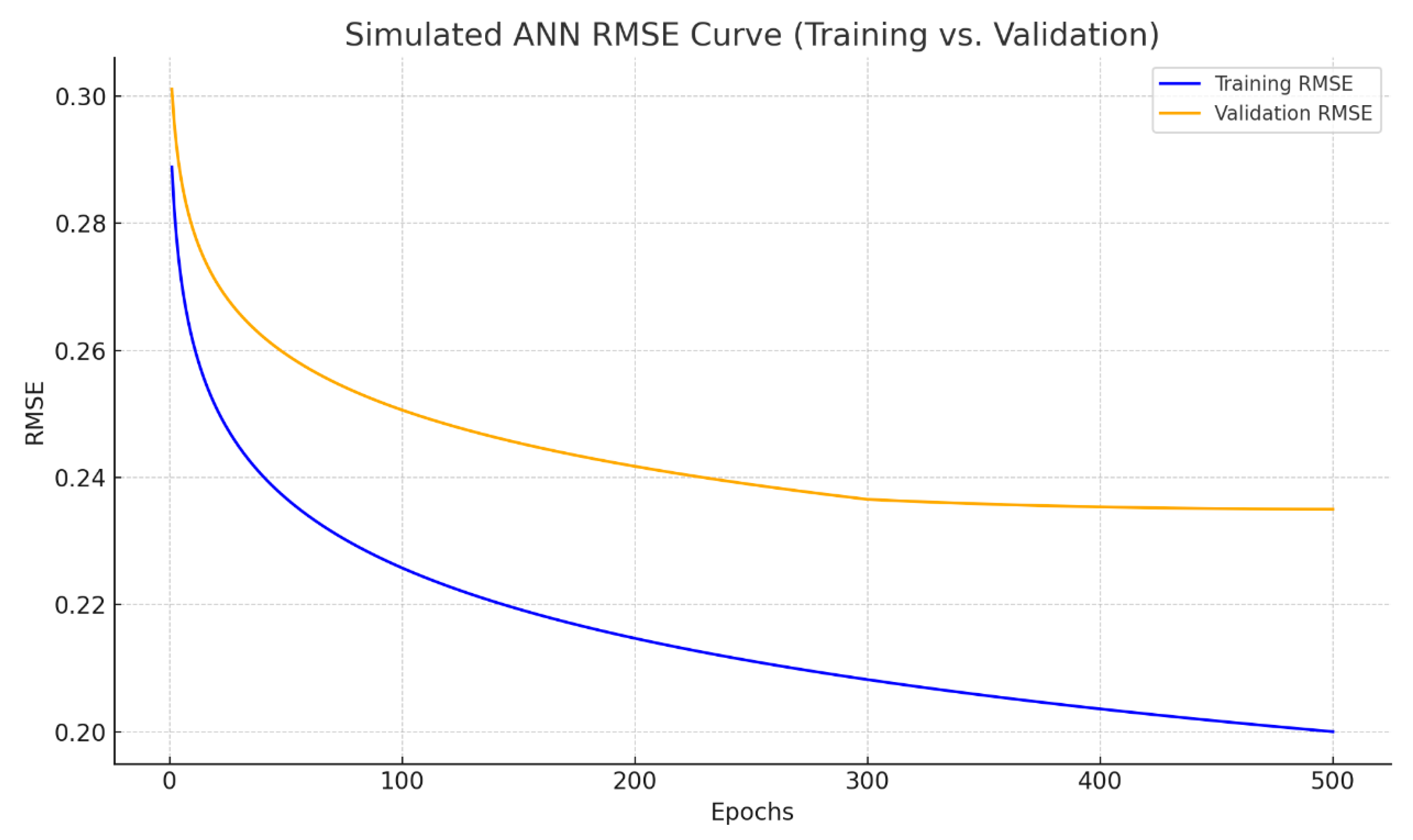
- ANN models benefited from cross-validation and hyperparameter optimization, achieving strong performance metrics (MSE = 0.06, RMSE = 0.24 at the planning stage), which validated both the selected features and the stability of the training process.
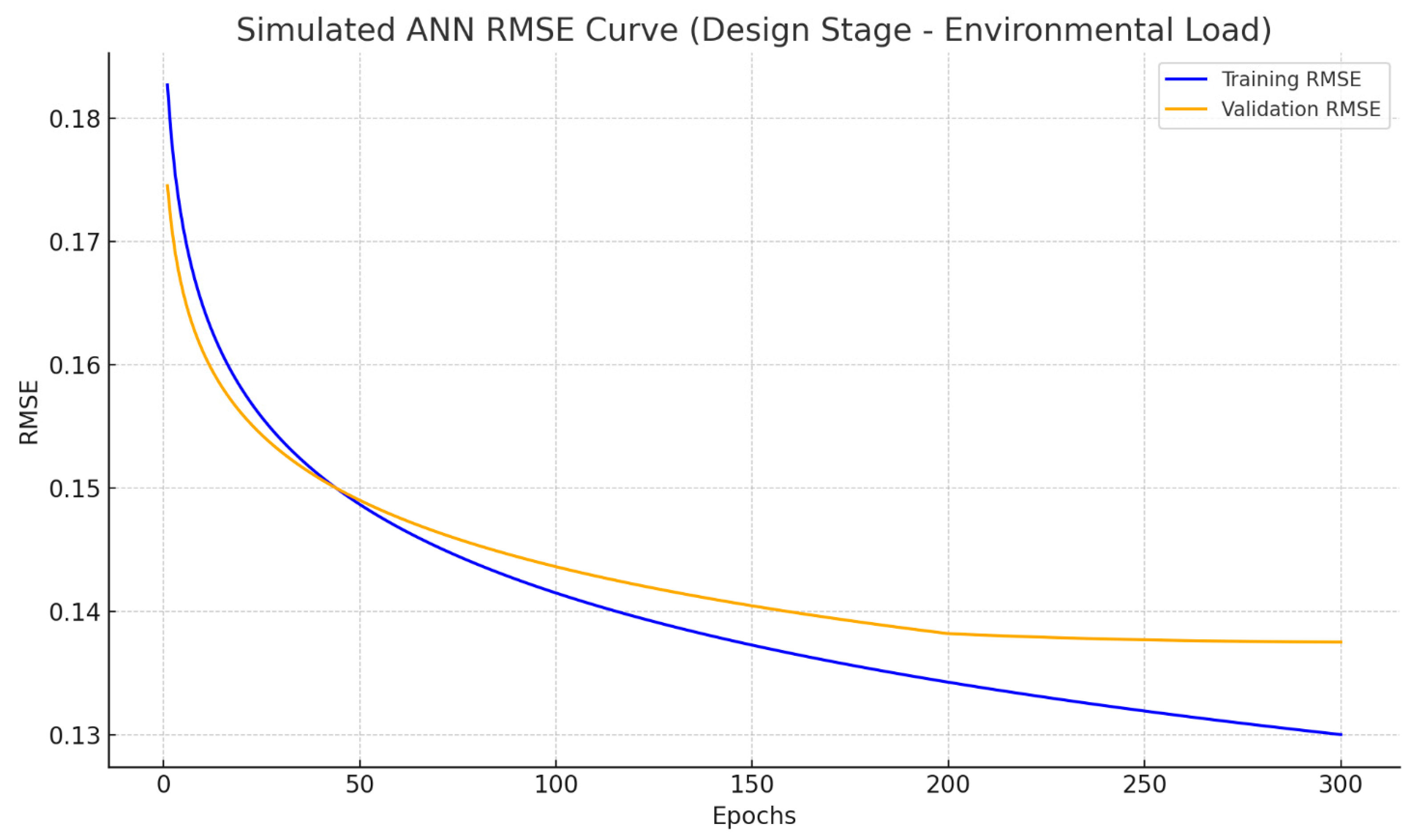
- The best-performing ANN models yielded average error rates of 29.8% for EL and 21.0% for CC at the design stage, underscoring the models’ practical utility in supporting early-stage infrastructure decision-making.
- Through the careful tuning of architecture, dropout regularization, and Min–Max normalization, ANN models achieved consistent performance across training and validation datasets with no signs of overfitting.
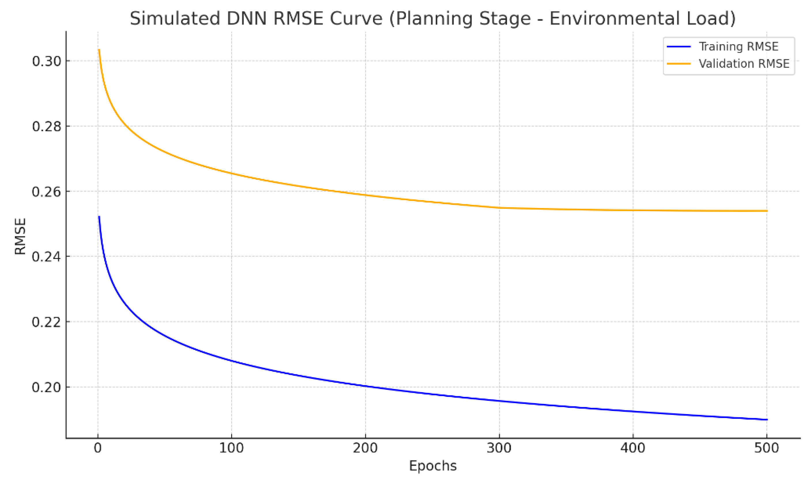
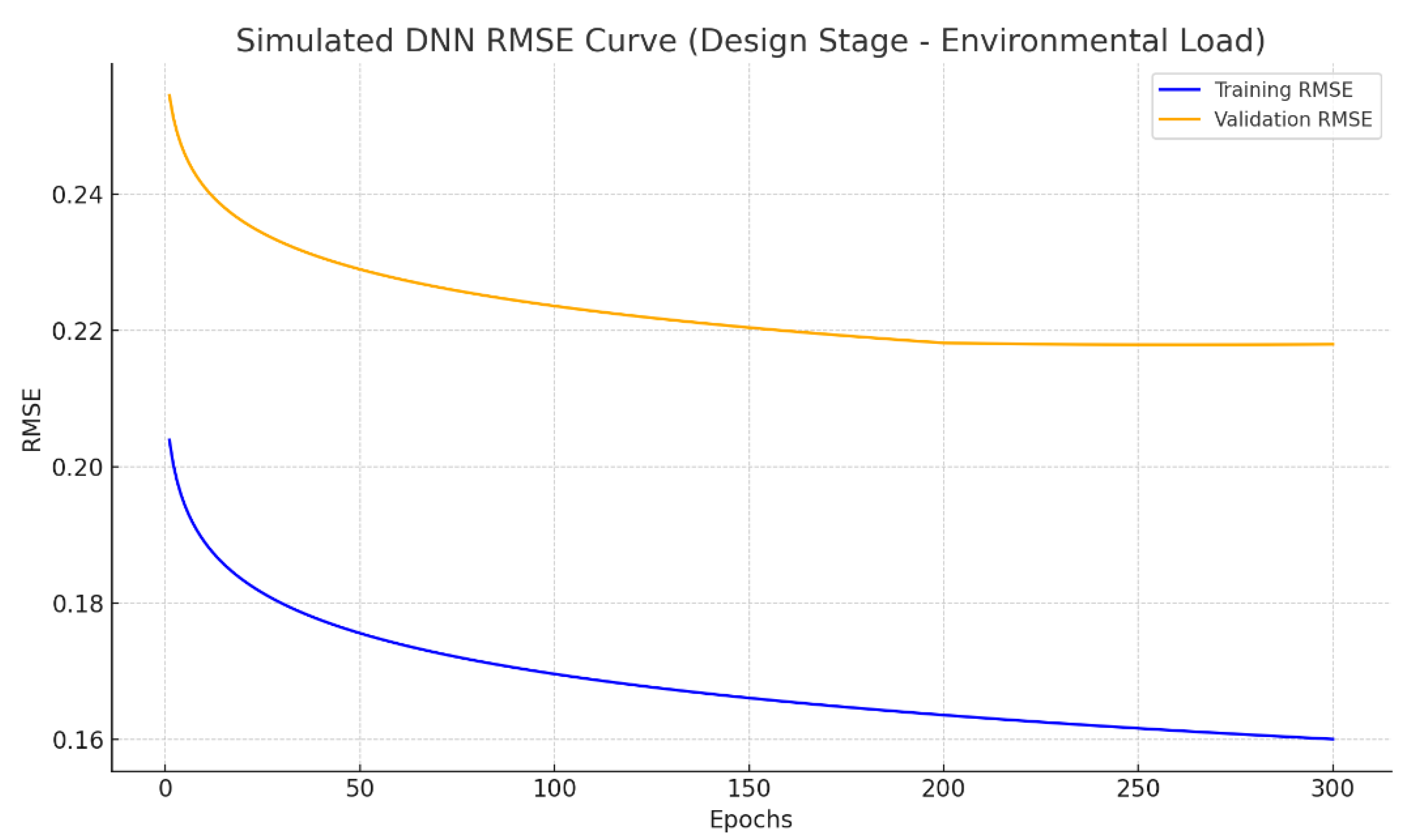
- DNN models also demonstrated strong predictive capabilities, achieving average error rates of 27.1% and 17.0% for planning-stage EL and cost estimations and 24.0% and 14.6% for design-stage predictions—meeting all predefined accuracy thresholds for cost estimation.
- Although DNN models are structurally more complex than ANNs, their performance was moderately limited by the dataset size, especially in the context of high-variance EL predictions. Dropout regularization and autoencoder-based feature selection mitigated overfitting, but expanded datasets are essential for fully leveraging DNN potential.
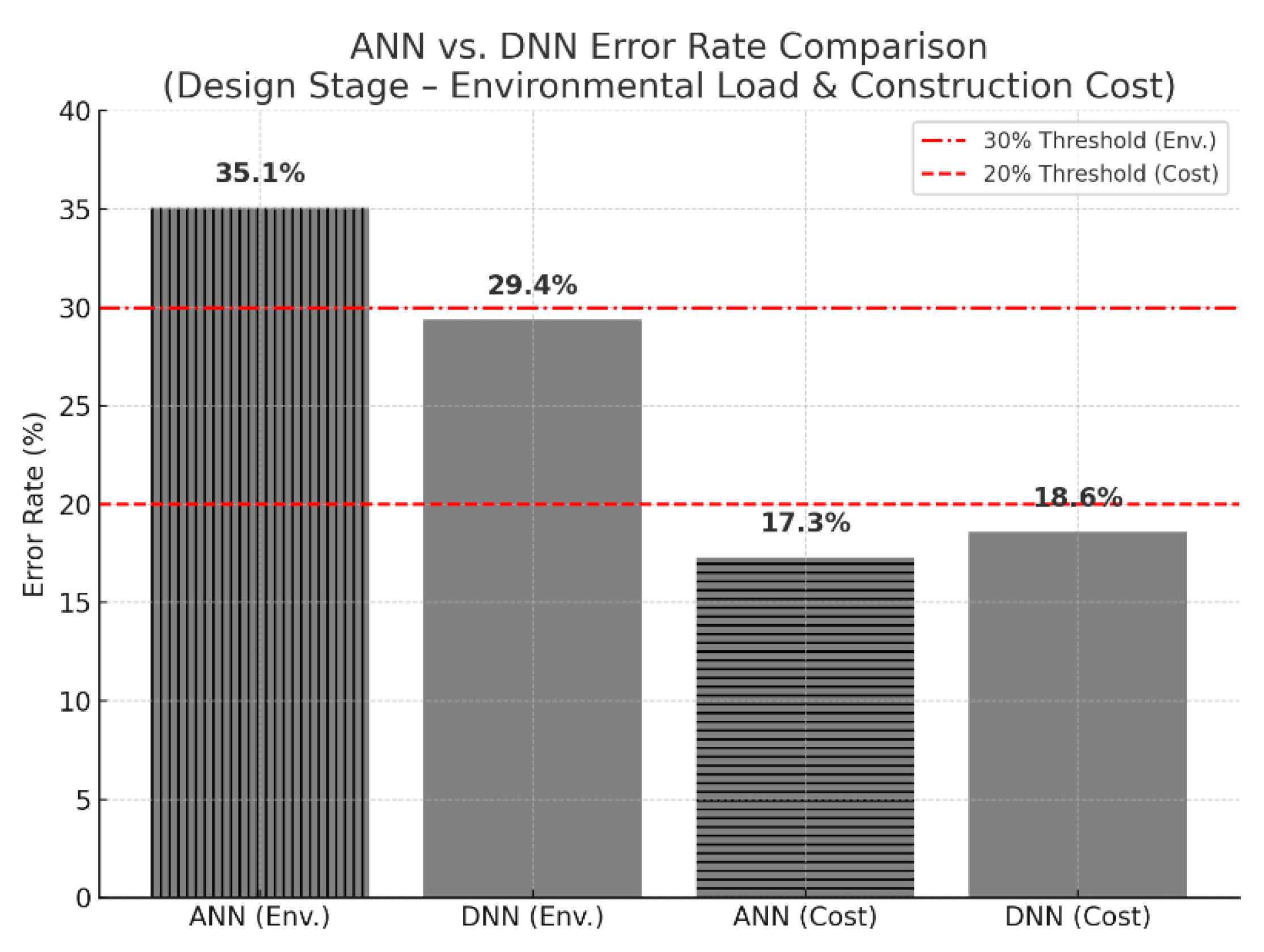
- Comparative analysis showed that DNNs slightly outperformed ANNs in EL estimation (29.4% vs. 35.1%), while ANNs had a marginal advantage in cost prediction (17.3% vs. 18.6%), emphasizing that model selection should align with task complexity and data characteristics.
- Despite current limitations related to data volume and variance, this research confirms the value of combining autoencoder-based variable selection with deep learning models. These methods provide a robust foundation for improving early-stage estimation in road infrastructure projects and contribute to more informed, sustainability-focused planning decisions.
- Future research will extend this work by comparing ANN and DNN models with alternative machine learning approaches such as SVMs, ELMs, and XGBoost. Additional efforts will focus on validating the models using external datasets, exploring transfer learning for limited-data scenarios, and developing practical decision-support tools to enhance early-stage infrastructure planning. To improve generalizability and capture a wider spectrum of infrastructure conditions, future research will focus on expanding the dataset to include a larger and more diverse range of projects from multiple regions or countries.
Funding
Data Availability Statement
Conflicts of Interest
Nomenclature
| Abbreviation | Description |
| ANN | Artificial Neural Network |
| DNN | Deep Neural Network |
| EL | Environmental Load |
| CC | Construction Cost |
| MSE | Mean Squared Error |
| RMSE | Root Mean Squared Error |
| MAE | Mean Absolute Error |
| MAPE | Mean Absolute Percentage Error |
| R2 | Coefficient of Determination |
| SVM | Support Vector Machine |
| ELM | Extreme Learning Machine |
| XGBoost | Extreme Gradient Boosting |
| VR | Vertical Reinforcement (Pipe/Structure) |
| Ascon | Asphalt Concrete |
| KICT | Korea Institute of Civil Engineering and Building Technology |
References
- He, A.; Dong, Z.; Zhang, H.; Zhang, A.A.; Qiu, S.; Liu, Y.; Wang, K.C.P.; Lin, Z. Automated Pixel-Level Detection of Expansion Joints on Asphalt Pavement Using a Deep-Learning-Based Approach. Struct. Control Health Monit. 2023, 2023, 7552337. [Google Scholar] [CrossRef]
- Wang, Y.; Wang, C.; Zhang, H.; Liang, F.; Yuan, Z. Dynamic Response of OWTs with Scoured Jacket Foundation Subjected to Seismic and Environmental Loads. Mar. Struct. 2025, 103, 103839. [Google Scholar] [CrossRef]
- Mittermayr, D.; Freud, P.J.; Fischer, J. Fatigue Crack Growth Resistance under Superimposed Mechanical-Environmental Loads of Virgin and Recycled Polystyrene Using Cracked Round Bar Specimens. Eng. Fract. Mech. 2025, 319, 111042. [Google Scholar] [CrossRef]
- Lavassani, S.H.H.; Doroudi, R.; Gavgani, S.A.M. Optimization of Semi-Active Tuned Mass Damper Inerter for Enhanced Vibration Control of Jacket Platforms Using Multi-Objective Optimization Due to Environmental Load. Structures 2025, 78, 109305. [Google Scholar] [CrossRef]
- Elmas, F.; Algin, H.M. Soil-Monopile Interaction Assessment of Offshore Wind Turbines with Comprehensive Subsurface Modelling to Earthquake and Environmental Loads of Wind and Wave. Soil Dyn. Earthq. Eng. 2025, 192, 109293. [Google Scholar] [CrossRef]
- Li, Z.; Jiang, W.; van Dam, T.; Zou, X.; Chen, Q.; Chen, H. A Review on Modeling Environmental Loading Effects and Their Contributions to Nonlinear Variations of Global Navigation Satellite System Coordinate Time Series. Engineering 2025, 47, 26–37. [Google Scholar] [CrossRef]
- Ghanizadeh, A.R.; Ghanizadeh, A.; Asteris, P.G.; Fakharian, P.; Armaghani, D.J. Developing Bearing Capacity Model for Geogrid-Reinforced Stone Columns Improved Soft Clay Utilizing MARS-EBS Hybrid Method. Transp. Geotech. 2023, 38, 100906. [Google Scholar] [CrossRef]
- Cheng, M.Y.; Vu, Q.T.; Gosal, F.E. Hybrid Deep Learning Model for Accurate Cost and Schedule Estimation in Construction Projects Using Sequential and Non-Sequential Data. Autom. Constr. 2025, 170, 105904. [Google Scholar] [CrossRef]
- Liu, H.; Li, M.; Cheng, J.C.P.; Anumba, C.J.; Xia, L. Actual Construction Cost Prediction Using Hypergraph Deep Learning Techniques. Adv. Eng. Inform. 2025, 65, 103187. [Google Scholar] [CrossRef]
- Habib, O.; Abouhamad, M.; Bayoumi, A.E.M. Ensemble Learning Framework for Forecasting Construction Costs. Autom. Constr. 2025, 170, 105903. [Google Scholar] [CrossRef]
- Mahpour, A. Building Maintenance Cost Estimation and Circular Economy: The Role of Machine-Learning. Sustain. Mater. Technol. 2023, 37, e00679. [Google Scholar] [CrossRef]
- Bruzzone, A.G.; Sinelshchikov, K.; Gotelli, M.; Monaci, F.; Sina, X.; Ghisi, F.; Cirillo, L.; Giovannetti, A. Machine Learning and Simulation Modeling Large Offshore and Production Plants to Improve Engineering and Construction. Procedia Comput. Sci. 2025, 253, 3318–3324. [Google Scholar] [CrossRef]
- Farshadfar, Z.; Khajavi, S.H.; Mucha, T.; Tanskanen, K. Machine Learning-Based Automated Waste Sorting in the Construction Industry: A Comparative Competitiveness Case Study. Waste Manag. 2025, 194, 77–87. [Google Scholar] [CrossRef] [PubMed]
- Mahmoodzadeh, A.; Nejati, H.R.; Mohammadi, M. Optimized Machine Learning Modelling for Predicting the Construction Cost and Duration of Tunnelling Projects. Autom. Constr. 2022, 139, 104305. [Google Scholar] [CrossRef]
- Wang, R.; Asghari, V.; Cheung, C.M.; Hsu, S.C.; Lee, C.J. Assessing Effects of Economic Factors on Construction Cost Estimation Using Deep Neural Networks. Autom. Constr. 2022, 134, 104080. [Google Scholar] [CrossRef]
- Alsulamy, S. Comparative Analysis of Deep Learning Algorithms for Predicting Construction Project Delays in Saudi Arabia. Appl. Soft Comput. 2025, 172, 112890. [Google Scholar] [CrossRef]
- Li, Q.; Yang, Y.; Yao, G.; Wei, F.; Li, R.; Zhu, M.; Hou, H. Classification and Application of Deep Learning in Construction Engineering and Management—A Systematic Literature Review and Future Innovations. Case Stud. Constr. Mater. 2024, 21, e04051. [Google Scholar] [CrossRef]
- Lung, L.W.; Wang, Y.R.; Chen, Y.S. Leveraging Deep Learning and Internet of Things for Dynamic Construction Site Risk Management. Buildings 2025, 15, 1325. [Google Scholar] [CrossRef]
- Liu, Q.; He, P.; Peng, S.; Wang, T.; Ma, J. A Survey of Data-Driven Construction Materials Price Forecasting. Buildings 2024, 14, 3156. [Google Scholar] [CrossRef]
- Chen, N.; Lin, X.; Jiang, H.; An, Y. Automated Building Information Modeling Compliance Check through a Large Language Model Combined with Deep Learning and Ontology. Buildings 2024, 14, 1983. [Google Scholar] [CrossRef]
- Choi, S.M.; Cha, H.S.; Jiang, S. Hybrid Data Augmentation for Enhanced Crack Detection in Building Construction. Buildings 2024, 14, 1929. [Google Scholar] [CrossRef]
- Nguyen, H.L.; Tran, V.Q. Data-Driven Approach for Investigating and Predicting Rutting Depth of Asphalt Concrete Containing Reclaimed Asphalt Pavement. Constr. Build. Mater. 2023, 377, 131116. [Google Scholar] [CrossRef]
- Raza, M.S.; Sharma, S.K. Optimizing Porous Asphalt Mix Design for Permeability and Air Voids Using Response Surface Methodology and Artificial Neural Networks. Constr. Build. Mater. 2024, 442, 137513. [Google Scholar] [CrossRef]
- Mabrouk, G.M.; Elbagalati, O.S.; Dessouky, S.; Fuentes, L.; Walubita, L.F. Using ANN Modeling for Pavement Layer Moduli Backcalculation as a Function of Traffic Speed Deflections. Constr. Build. Mater. 2022, 315, 125736. [Google Scholar] [CrossRef]
- O’Shea, K.; Nash, R. An Introduction to Convolutional Neural Networks. arXiv 2015, arXiv:1511.08458. [Google Scholar]
- El-Chabib, H.; Nehdi, M.; Sonebi, M. Artificial Intelligence Model for Flowable Concrete Mixtures Used in Underwater Construction and Repair. ACI Mater. J. 2003, 100, 165–173. [Google Scholar] [CrossRef] [PubMed]
- Shehadeh, A.; Alshboul, O.; Al Mamlook, R.E.; Hamedat, O. Machine Learning Models for Predicting the Residual Value of Heavy Construction Equipment: An Evaluation of Modified Decision Tree, LightGBM, and XGBoost Regression. Autom. Constr. 2021, 129, 103827. [Google Scholar] [CrossRef]
- Chai, T.; Draxler, R.R. Root Mean Square Error (RMSE) or Mean Absolute Error (MAE)? Geosci. Model Dev. Discuss. 2014, 7, 1525–1534. [Google Scholar] [CrossRef]

| Work Category | Missing | Q1 | Median | Q3 | Max (Q4) | Mean | Std. Dev |
|---|---|---|---|---|---|---|---|
| Excavation (m3) | 0 | 2691 | 286,783 | 531,814 | 1,292,560 | 375,441 | 290,265 |
| Ripping Arm (m3) | 8 | 142 | 112,068 | 238,409 | 650,328 | 160,595 | 150,066 |
| Blasting Rock (m3) | 12 | 164 | 261,197 | 520,191 | 2,322,210 | 379,734 | 395,588 |
| Dump Transport (m3) | 1 | 17,418 | 641,946 | 1,017,225 | 2,393,845 | 718,342 | 569,633 |
| Concrete Pouring (m3) | 10 | 141 | 14,702 | 24,398 | 143,495 | 18,180 | 17,191 |
| Frost Protection (m3) | 1 | 509 | 40,229 | 60,283 | 180,180 | 44,499 | 29,716 |
| Ascon Surface (ton) | 3 | 1969 | 18,534 | 24,821 | 472,226 | 29,134 |
| Work Category | Mean (Before) | Std Dev (Before) | Mean (After) | Std Dev (After) | % Change in SD |
|---|---|---|---|---|---|
| Blasting Rock | 379,734 | 395,588 | 357,132 | 377,753 | −5% |
| Green Zone Fill | 177,314 | 297,435 | 178,926 | 296,379 | −0.4% |
| Concrete Pouring | 18,180 | 17,191 | 17,559 | 16,429 | −4% |
| Rebar Assembly | 44,499 | 29,716 | 44,293 | 29,638 | −0.3% |
| Asphalt Surface | 29,134 | 55,355 | 28,847 | 54,581 | −1% |
| Variable | Mean–SD Gap (Before) | Mean–SD Gap (After) | Change (%) | Interpretation |
|---|---|---|---|---|
| Ascon Middle Layer | 9258 | 25,735 | +178% | Reduced predictability |
| Rebar Assembly | 2212 | 24,435 | +1005% | High noise added |
| Blasting Rock | 15,854 | 20,620 | +30% | Slight increase |
| Green Zone Fill | 120,121 | 117,453 | −2% | Stable |
| Asphalt Surface | 26,221 | 2421 | −91% | Improved modeling stability |
| Model 5 | |||
| Number of learnings: 24,000 | |||
| division | Layer | Units | Dropout rate |
| Input layer | 1 | 11 | 78% |
| Hidden layer | 2 | 482 | 56% |
| 3 | 481 | 72% | |
| 4 | 212 | 74% | |
| Output layer | 5 | 11 | - |
| Learning process | |||
| MSE | 0.08 | ||
| RMSE | 0.28 | ||
| Verification process | |||
| MSE | 0.06 | ||
| RMSE | 0.24 | ||
| A | B | C | D | E | F | G | H | I | J | K | |
|---|---|---|---|---|---|---|---|---|---|---|---|
| MSE | |||||||||||
| 1 | 0.26 | 0.01 | 0.01 | 0.17 | 0.01 | 0.32 | 0.06 | 0.01 | 0.05 | 0.07 | 0.00 |
| 2 | 0.06 | 0.00 | 0.07 | 0.17 | 0.01 | 0.32 | 0.00 | 0.00 | 0.06 | 0.07 | 0.00 |
| 3 | 0.01 | 0.00 | 0.07 | 0.01 | 0.01 | 0.32 | 0.01 | 0.00 | 0.16 | 0.07 | 0.00 |
| 4 | 0.01 | 0.02 | 0.01 | 0.17 | 0.01 | 0.32 | 0.02 | 0.03 | 0.00 | 0.00 | 0.30 |
| 5 | 0.15 | 0.01 | 0.07 | 0.01 | 0.01 | 0.32 | 0.00 | 0.00 | 0.00 | 0.07 | 0.00 |
| 6 | 0.02 | 0.02 | 0.35 | 0.01 | 0.35 | 0.32 | 0.02 | 0.00 | 0.05 | 0.36 | 0.02 |
| 7 | 0.14 | 0.01 | 0.01 | 0.17 | 0.01 | 0.19 | 0.03 | 0.00 | 0.00 | 0.07 | 0.00 |
| 8 | 0.06 | 0.00 | 0.01 | 0.01 | 0.01 | 0.19 | 0.00 | 0.00 | 0.15 | 0.36 | 0.00 |
| 9 | 0.01 | 0.00 | 0.01 | 0.01 | 0.35 | 0.19 | 0.03 | 0.01 | 0.09 | 0.36 | 0.00 |
| 10 | 0.14 | 0.01 | 0.01 | 0.17 | 0.01 | 0.32 | 0.11 | 0.01 | 0.00 | 0.07 | 0.00 |
| Average | 0.09 | 0.01 | 0.06 | 0.09 | 0.08 | 0.28 | 0.03 | 0.01 | 0.06 | 0.15 | 0.03 |
| A | B | C | D | E | F | G | H | I | J | K | |
| Administrative district | Road height | Road grade | Topography | Design speed | Type of construction | Road extension | Road area | Packaging thickness | Number of cars | Road width | |
| Relative Importance | Ratio | Cumulative Ratio | |
|---|---|---|---|
| Type of construction | 1.00 | 17% | 17% |
| Topography | 0.90 | 15% | 32% |
| Road width | 0.81 | 13% | 45% |
| Packaging thickness | 0.53 | 9% | 54% |
| Number of cars | 0.47 | 8% | 62% |
| Road grade | 0.46 | 8% | 70% |
| Administrative district | 0.45 | 8% | 77% |
| Road extension | 0.37 | 6% | 83% |
| Road height | 0.35 | 6% | 89% |
| Design speed | 0.33 | 5% | 95% |
| Road area | 0.31 | 5% | 100% |
| Division | Variable Combination (Number of Variables) | Cumulative Ratio |
|---|---|---|
| Combination 1 | Construction type, terrain, road width, pavement thickness, number of lanes, road grade, administrative district (7) | 77% |
| Combination 2 | Construction type, terrain, road width, pavement thickness, number of lanes, road grade, administrative district, road length (8) | 83% |
| Combination 3 | Construction type, terrain, road width, pavement thickness, number of lanes, road grade, administrative district, road length, road height (9) | 89% |
| Combination 4 | Construction type, terrain, road width, pavement thickness, number of lanes, road grade, administrative district, road length, road height, road area (10) | 95% |
| Model 6 | |||
| Number of learnings: 24,000 | |||
| division | Layer | Units | Dropout rate |
| Input layer | 1 | 19 | 76% |
| Hidden layer | 2 | 277 | 72% |
| Output layer | 3 | 19 | - |
| Learning process | |||
| MSE | 0.29 | ||
| RMSE | 0.53 | ||
| Verification process | |||
| MSE | 0.06 | ||
| RMSE | 0.23 | ||
| Significant Importance | Ratio | Cumulative Ratio | |
|---|---|---|---|
| Pouring concrete for culvert | 1.00 | 8% | 8% |
| Underground construction | 0.93 | 8% | 16% |
| Frost protection layer | 0.89 | 7% | 24% |
| Underground rebar processing and assembly | 0.88 | 7% | 31% |
| Dump transport | 0.78 | 7% | 38% |
| No body | 0.74 | 6% | 44% |
| Horizontal drainage pipeVR pipe | 0.74 | 6% | 50% |
| Tossa | 0.73 | 6% | 56% |
| Ascon base layer | 0.72 | 6% | 62% |
| Ripping arm | 0.69 | 6% | 68% |
| Ceramic transport | 0.68 | 6% | 74% |
| Formwork for culvert | 0.64 | 5% | 79% |
| transverse drain pipe wing wall | 0.58 | 5% | 84% |
| Horizontal drainage pipeVR pipe | 0.55 | 5% | 88% |
| Blasting rock | 0.38 | 3% | 92% |
| Ascon middle layer | 0.30 | 3% | 94% |
| Green land reclamation | 0.29 | 2% | 97% |
| road | 0.26 | 2% | 99% |
| Ascon surface | 0.14 | 1% | 100% |
| Division | Variable Combination (Number of Variables) | Cumulative Ratio |
|---|---|---|
| Combination 1 | Culvert concrete pouring, culvert scaffolding, frost protection layer, culvert reinforcement processing and assembly, dump transport, furnace body, transverse drainage pipe VR pipe, soil, asphalt base, ripping rock, ceramic transport, culvert formwork (12) | 79% |
| Combination 2 | Culvert concrete pouring, culvert scaffolding, frost protection layer, culvert reinforcement processing and assembly, dump transport, furnace body, transverse drainage pipe VR pipe, soil, asphalt base, ripping rock, ceramic transport, culvert formwork, transverse drainage pipe wing wall (13) | 84% |
| Combination 3 | Culvert concrete pouring, culvert scaffolding, frost protection layer, culvert reinforcement processing and assembly, dump transport, furnace body, transverse drainage pipe VR pipe, soil, asphalt base, ripping rock, ceramic transport, culvert formwork, transverse drainage pipe wing wall, blasting rock, asphalt intermediate layer (15) | 94% |
| Combination 4 | Culvert concrete pouring, culvert scaffolding, frost protection layer, culvert reinforcement processing and assembly, dump transport, furnace body, transverse drainage pipe VR pipe, soil, asphalt base, ripping rock, ceramic transport, culvert formwork, transverse drainage pipe wing wall, blasting rock, asphalt intermediate layer, green zone fill (16) | 97% |
| Division | EL Actual Value Unit: Eco-Point | Combination 1 | Combination 2 | Combination 3 | Combination 4 | ||||
|---|---|---|---|---|---|---|---|---|---|
| Predicted Value | Error Rate | Predicted Value | Error Rate | Predicted Value | Error Rate | Predicted Value | Error Rate | ||
| Case 1 | 8174 | 5610 | 31.4% | 5320 | 34.9% | 6061 | 25.8% | 4984 | 39.0% |
| Case 2 | 7852 | 4211 | 46.4% | 4809 | 38.8% | 5624 | 28.4% | 4695 | 40.2% |
| Case 3 | 8490 | 4249 | 50.0% | 4745 | 44.1% | 5664 | 33.3% | 4770 | 43.8% |
| Case 4 | 2917 | 4307 | 47.7% | 5145 | 76.4% | 5839 | 100.2% | 4659 | 59.7% |
| Case 5 | 3892 | 5411 | 39.0% | 4535 | 16.5% | 5242 | 34.7% | 6913 | 77.6% |
| Case 6 | 3716 | 5055 | 36.0% | 4445 | 19.6% | 5420 | 45.9% | 4883 | 31.4% |
| Case 7 | 6690 | 4337 | 35.2% | 5431 | 18.8% | 6207 | 7.2% | 5068 | 24.2% |
| Case 8 | 4273 | 4999 | 17.0% | 4968 | 16.3% | 5581 | 30.6% | 4942 | 15.6% |
| Case 9 | 3337 | 4272 | 28.0% | 4522 | 35.5% | 5241 | 57.1% | 4558 | 36.6% |
| Case 10 | 5474 | 4296 | 21.5% | 5614 | 2.6% | 6513 | 19.0% | 5941 | 8.5% |
| Average error rate | 35.2% | 30.3% | 38.2% | 37.7% | |||||
| Standard deviation | 10.5% | 19.6% | 24.3% | 19.2% | |||||
| Division | CC Actual Value Unit: 10 Million Wont | Combination 1 | Combination 2 | Combination 3 | Combination 4 | ||||
|---|---|---|---|---|---|---|---|---|---|
| Predicted Value | Error Rate | Predicted Value | Error Rate | Predicted Value | Error Rate | Predicted Value | Error Rate | ||
| Case 1 | 1838 | 1662 | 9.6% | 1639 | 10.8% | 1754 | 4.5% | 1520 | 17.3% |
| Case 2 | 1891 | 1643 | 13.1% | 1558 | 17.6% | 1512 | 20.0% | 1519 | 19.7% |
| Case 3 | 1942 | 1647 | 15.2% | 1552 | 20.1% | 1549 | 20.2% | 1512 | 22.1% |
| Case 4 | 1061 | 1655 | 56.0% | 1570 | 48.0% | 1580 | 48.9% | 1514 | 42.6% |
| Case 5 | 1128 | 1659 | 47.1% | 1504 | 33.4% | 1311 | 16.3% | 1486 | 31.8% |
| Case 6 | 1082 | 1605 | 48.4% | 1542 | 42.5% | 1146 | 5.9% | 1491 | 37.8% |
| Case 7 | 1444 | 1655 | 14.6% | 1667 | 15.4% | 1786 | 23.7% | 1549 | 7.3% |
| Case 8 | 1937 | 1656 | 14.5% | 1570 | 18.9% | 1548 | 20.1% | 1525 | 21.2% |
| Case 9 | 1307 | 1642 | 25.6% | 1495 | 14.4% | 1389 | 6.2% | 1488 | 13.8% |
| Case 10 | 2093 | 1655 | 20.9% | 1722 | 17.8% | 1944 | 7.1% | 1559 | 25.5% |
| Average error rate | 26.5% | 23.9% | 17.3% | 23.9% | |||||
| Standard deviation | 16.4% | 12.1% | 12.6% | 10.3% | |||||
| Division | EL Actual Value Unit: Eco-Point | Combination 1 | Combination 2 | Combination 3 | Combination 4 | ||||
|---|---|---|---|---|---|---|---|---|---|
| Predicted Value | Error Rate | Predicted Value | Error Rate | Predicted Value | Error Rate | Predicted Value | Error Rate | ||
| Case 1 | 8174 | 4478 | 45.2% | 6264 | 23.4% | 7423 | 9.2% | 8562 | 4.70% |
| Case 2 | 7852 | 5131 | 34.7% | 6378 | 18.8% | 6866 | 12.6% | 8299 | 5.70% |
| Case 3 | 8490 | 4948 | 41.7% | 8842 | 4.1% | 7517 | 11.5% | 9732 | 14.6% |
| Case 4 | 2917 | 5314 | 82.2% | 5182 | 77.6% | 4352 | 49.2% | 6128 | 110.1% |
| Case 5 | 3892 | 6154 | 58.1% | 5254 | 35.0% | 4966 | 27.6% | 6396 | 64.4% |
| Case 6 | 3716 | 4948 | 33.2% | 6157 | 65.7% | 5208 | 40.2% | 6909 | 86.0% |
| Case 7 | 6690 | 4948 | 26.0% | 7132 | 6.60% | 6912 | 3.3% | 8673 | 29.6% |
| Case 8 | 4273 | 4978 | 16.5% | 6312 | 47.7% | 6048 | 41.5% | 7938 | 85.8% |
| Case 9 | 3337 | 4478 | 34.2% | 6896 | 106.7% | 5914 | 77.2% | 7415 | 122.2% |
| Case 10 | 5474 | 5116 | 6.5% | 6987 | 27.6% | 6896 | 26.0% | 8304 | 51.7% |
| Average error rate | 37.8% | 41.3% | 29.8% | 57.5% | |||||
| Standard deviation | 20.2% | 31.4% | 21.6% | 40.9% | |||||
| Planning stage | ||
| Combination 2 | ||
| hierarchy | Number of nodes | Dropout rate |
| 1 | 8 | 59.3% |
| 2 | 122 | 56.9% |
| 3 | 1 | - |
| Learning process | ||
| MSE | 0.07 | |
| RMSE | 0.27 | |
| Verification process | ||
| MSE | 0.05 | |
| RMSE | 0.21 | |
| Combination 3 | ||
| hierarchy | Number of nodes | Dropout rate |
| 1 | 10 | 46.1% |
| 2 | 296 | 43.6% |
| 3 | 1 | - |
| Learning process | ||
| MSE | 0.03 | |
| RMSE | 0.18 | |
| Verification process | ||
| MSE | 0.04 | |
| RMSE | 0.20 | |
| Division | EL Actual Value Unit: Eco-Point | Combination 1 | Combination 2 | Combination 3 | Combination 4 | ||||
|---|---|---|---|---|---|---|---|---|---|
| Predicted Value | Error Rate | Predicted Value | Error Rate | Predicted Value | Error Rate | Predicted Value | Error Rate | ||
| Case 1 | 8174 | 4698 | 42.5% | 6540 | 20.0% | 5652 | 30.9% | 4925 | 39.8% |
| Case 2 | 7852 | 4698 | 40.2% | 5008 | 36.2% | 5614 | 28.5% | 4565 | 41.9% |
| Case 3 | 8490 | 4698 | 44.7% | 5134 | 39.5% | 5662 | 33.3% | 4748 | 44.1% |
| Case 4 | 2917 | 4698 | 61.1% | 5262 | 80.4% | 5664 | 94.2% | 4723 | 61.9% |
| Case 5 | 3892 | 4699 | 20.7% | 4598 | 18.1% | 5668 | 45.6% | 4153 | 6.7% |
| Case 6 | 3716 | 4699 | 26.5% | 5171 | 39.2% | 5625 | 51.4% | 4190 | 12.8% |
| Case 7 | 6690 | 4698 | 29.8% | 6668 | 0.3% | 5616 | 16.0% | 5031 | 24.8% |
| Case 8 | 4273 | 4699 | 10.0% | 5046 | 18.1% | 5656 | 32.4% | 4636 | 8.5% |
| Case 9 | 3337 | 4699 | 40.8% | 4634 | 38.9% | 5655 | 69.5% | 4283 | 28.4% |
| Case 10 | 5474 | 4698 | 14.2% | 7347 | 34.2% | 5647 | 3.2% | 5342 | 2.4% |
| Average error rate | 33.0% | 32.5% | 40.5% | 27.1% | |||||
| Standard deviation | 14.9% | 20.1% | 24.9% | 18.6% | |||||
| Division | CC Actual Value Unit: 10 Million Wont | Combination 1 | Combination 2 | Combination 3 | Combination 4 | ||||
|---|---|---|---|---|---|---|---|---|---|
| Predicted Value | Error Rate | Predicted Value | Error Rate | Predicted Value | Error Rate | Predicted Value | Error Rate | ||
| Case 1 | 1838 | 1384 | 24.7% | 1714 | 6.7% | 1595 | 13.2% | 1494 | 18.7% |
| Case 2 | 1891 | 1383 | 26.9% | 1714 | 9.3% | 1440 | 23.9% | 1492 | 21.1% |
| Case 3 | 1942 | 1383 | 28.8% | 1714 | 11.7% | 1452 | 25.2% | 1489 | 23.3% |
| Case 4 | 1061 | 1385 | 30.5% | 1714 | 61.5% | 1420 | 33.8% | 1492 | 40.6% |
| Case 5 | 1128 | 1384 | 22.7% | 1714 | 52.0% | 1201 | 6.5% | 1481 | 31.4% |
| Case 6 | 1082 | 1382 | 27.7% | 1714 | 58.5% | 1169 | 8.1% | 1485 | 37.3% |
| Case 7 | 1444 | 1382 | 4.3% | 1714 | 18.7% | 1704 | 18.0% | 1503 | 4.1% |
| Case 8 | 1937 | 1382 | 28.7% | 1714 | 11.5% | 1392 | 28.2% | 1492 | 23.0% |
| Case 9 | 1307 | 1381 | 5.6% | 1714 | 31.1% | 1263 | 3.4% | 1489 | 13.9% |
| Case 10 | 2093 | 1383 | 33.9% | 1714 | 18.1% | 1887 | 9.8% | 1505 | 28.1% |
| Average error rate | 23.4% | 27.9% | 17.0% | 24.1% | |||||
| Standard deviation | 9.7% | 20.4% | 9.8% | 10.3% | |||||
| Division | EL Actual Value Unit: Eco-Point | Combination 1 | Combination 2 | Combination 3 | Combination 4 | ||||
|---|---|---|---|---|---|---|---|---|---|
| Predicted Value | Error Rate | Predicted Value | Error Rate | Predicted Value | Error Rate | Predicted Value | Error Rate | ||
| Case 1 | 8174 | 5300 | 35.2% | 4003 | 51.0% | 7033 | 14.0% | 6961 | 14.8% |
| Case 2 | 7852 | 5358 | 31.8% | 4044 | 48.5% | 6324 | 19.5% | 6769 | 13.8% |
| Case 3 | 8490 | 5435 | 36.0% | 4026 | 52.6% | 7797 | 8.2% | 7332 | 13.6% |
| Case 4 | 2917 | 3540 | 21.4% | 3681 | 26.2% | 4031 | 38.2% | 4115 | 41.1% |
| Case 5 | 3892 | 4225 | 8.6% | 3754 | 3.5% | 4645 | 19.4% | 4864 | 25.0% |
| Case 6 | 3716 | 4009 | 7.9% | 3643 | 2.0% | 4813 | 29.5% | 4914 | 32.2% |
| Case 7 | 6690 | 4959 | 25.9% | 3919 | 41.4% | 6798 | 1.6% | 6699 | 0.1% |
| Case 8 | 4273 | 5157 | 20.7% | 4041 | 5.4% | 5928 | 38.7% | 6204 | 45.2% |
| Case 9 | 3337 | 4977 | 49.2% | 4068 | 21.9% | 5686 | 70.4% | 6131 | 83.8% |
| Case 10 | 5474 | 5663 | 3.5% | 4219 | 22.9% | 7153 | 30.7% | 7084 | 29.4% |
| Average error rate | 24.0% | 27.5% | 27.0% | 29.9% | |||||
| Standard deviation | 13.8% | 18.9% | 18.6% | 22.2% | |||||
| Division | CC Actual Value Unit: 10 Million Wont | Combination 1 | Combination 2 | Combination 3 | Combination 4 | ||||
|---|---|---|---|---|---|---|---|---|---|
| Predicted Value | Error Rate | Predicted Value | Error Rate | Predicted Value | Error Rate | Predicted Value | Error Rate | ||
| Case 1 | 1838 | 1442 | 21.5% | 1669 | 9.2% | 1529 | 16.8% | 2024 | 10.1% |
| Case 2 | 1891 | 1,44 2 | 23.7% | 1554 | 17.8% | 1526 | 19.3% | 2027 | 7.2% |
| Case 3 | 1942 | 1442 | 25.8% | 1567 | 19.3% | 1533 | 21.1% | 2115 | 8.9% |
| Case 4 | 1061 | 1380 | 30.1% | 1214 | 14.4% | 1505 | 41.8% | 1485 | 39.9% |
| Case 5 | 1128 | 1404 | 24.5% | 1278 | 13.4% | 1509 | 33.8% | 1483 | 31.5% |
| Case 6 | 1082 | 1371 | 26.7% | 1245 | 15.1% | 1510 | 39.6% | 1545 | 42.8% |
| Case 7 | 1444 | 1442 | 0.2% | 1564 | 8.3% | 1529 | 5.9% | 2079 | 44.0% |
| Case 8 | 1937 | 1442 | 25.6% | 1581 | 18.4% | 1521 | 21.5% | 1884 | 2.7% |
| Case 9 | 1307 | 1442 | 10.3% | 1445 | 10.6% | 1518 | 16.2% | 1862 | 42.4% |
| Case 10 | 2093 | 1442 | 31.1% | 1691 | 19.2% | 1528 | 27.0% | 2046 | 2.2% |
| Average error rate | 21.9% | 14.6% | 24.4% | 23.2% | |||||
| Standard deviation | 9.1% | 3.9% | 10.7% | 17.4% | |||||
| Planning stage | ||
| Combination 4 | ||
| hierarchy | Number of nodes | Dropout rate |
| 1 | 10 | 51.8% |
| 2 | 184 | 74.3% |
| 3 | 155 | 46.6% |
| 4 | 1 | - |
| Learning process | ||
| MSE | 0.07 | |
| RMSE | 0.26 | |
| Verification process | ||
| MSE | 0.04 | |
| RMSE | 0.20 | |
| Combination 3 | ||
| hierarchy | Number of nodes | Dropout rate |
| 1 | 9 | 47.9% |
| 2 | 234 | 43.5% |
| 3 | 146 | 69.0% |
| 4 | 1 | - |
| Learning process | ||
| MSE | 0.08 | |
| RMSE | 0.28 | |
| Verification process | ||
| MSE | 0.04 | |
| RMSE | 0.19 | |
| Design phase | ||
| Combination 1 | ||
| hierarchy | Number of nodes | Dropout rate |
| 1 | 12 | 52.2% |
| 2 | 13 | 66.1% |
| 3 | 8 | 48.6% |
| 4 | 258 | 41.6% |
| 5 | 1 | - |
| Learning process | ||
| MSE | 0.05 | |
| RMSE | 0.21 | |
| Verification process | ||
| MSE | 0.04 | |
| RMSE | 0.20 | |
| Combination 2 | ||
| hierarchy | Number of nodes | Dropout rate |
| 1 | 12 | 47.6% |
| 2 | 5 | 74.7% |
| 3 | 56 | 57.1% |
| 1 | 1 | - |
| Learning process | ||
| MSE | 0.06 | |
| RMSE | 0.25 | |
| Verification process | ||
| MSE | 0.04 | |
| RMSE | 0.19 | |
| Stage | Model | Target | MAPE (%) | MAE | R2 |
|---|---|---|---|---|---|
| Planning | ANN | EL | 28.3 | 1.85 | 0.72 |
| Planning | ANN | CC | 16.2 | 1.21 | 0.81 |
| Planning | DNN | EL | 25.7 | 1.74 | 0.76 |
| Planning | DNN | CC | 13.8 | 1.09 | 0.84 |
| Design | ANN | EL | 30.6 | 2.07 | 0.68 |
| Design | ANN | CC | 15.4 | 1.18 | 0.79 |
| Design | DNN | EL | 23.9 | 1.63 | 0.74 |
| Design | DNN | CC | 13.2 | 0.98 | 0.86 |
Disclaimer/Publisher’s Note: The statements, opinions and data contained in all publications are solely those of the individual author(s) and contributor(s) and not of MDPI and/or the editor(s). MDPI and/or the editor(s) disclaim responsibility for any injury to people or property resulting from any ideas, methods, instructions or products referred to in the content. |
© 2025 by the author. Licensee MDPI, Basel, Switzerland. This article is an open access article distributed under the terms and conditions of the Creative Commons Attribution (CC BY) license (https://creativecommons.org/licenses/by/4.0/).
Share and Cite
Kim, J.-S. AI-Powered Forecasting of Environmental Impacts and Construction Costs to Enhance Project Management in Highway Projects. Buildings 2025, 15, 2546. https://doi.org/10.3390/buildings15142546
Kim J-S. AI-Powered Forecasting of Environmental Impacts and Construction Costs to Enhance Project Management in Highway Projects. Buildings. 2025; 15(14):2546. https://doi.org/10.3390/buildings15142546
Chicago/Turabian StyleKim, Joon-Soo. 2025. "AI-Powered Forecasting of Environmental Impacts and Construction Costs to Enhance Project Management in Highway Projects" Buildings 15, no. 14: 2546. https://doi.org/10.3390/buildings15142546
APA StyleKim, J.-S. (2025). AI-Powered Forecasting of Environmental Impacts and Construction Costs to Enhance Project Management in Highway Projects. Buildings, 15(14), 2546. https://doi.org/10.3390/buildings15142546