Comprehensive Assessment of Indoor Thermal in Vernacular Building Using Machine Learning Model with GAN-Based Data Imputation: A Case of Aceh Region, Indonesia

Abstract

This study introduces a predictive model for estimating indoor room temperatures in vernacular building using external environmental factors such as air temperature, humidity, sunshine duration, and wind speed. The dataset was sourced from the Meteorology, Climatology, and Geophysics Agency and supplemented with direct measurements collected from four rooms within a vernacular building in Aceh Province, Indonesia. A Generative Adversarial Network (GAN)-based imputation technique was implemented to address missing data during preprocessing. The prediction model adopts a hybrid framework that integrates Multiple Linear Regression (MLR) and Artificial Neural Networks (ANNs), with both models optimized using Support Vector Regression (SVR) to better capture the nonlinear dynamics between inputs and outputs. The evaluation results show that the ANN-SVR model achieved the lowest average $\overline{MAE}$ and $\overline{RMSE}$ values, at 0.164 and 0.218, respectively, and the highest average $\overline{R}$ and $\overline{R^2}$ values, at 0.785 and 0.618. Evaluation results indicate that the ANN-SVR model consistently achieved the lowest error rates and the highest correlation coefficients across all four rooms, identifying it as the most effective model for forecasting indoor thermal conditions. These results validate the combined use of ANN-SVR for prediction and GAN for preprocessing as a powerful strategy to enhance data quality and model performance. The findings offer a scientific basis for architectural planning to improve thermal comfort in vernacular buildings such as the Rumoh Aceh.

1. Introduction

A vernacular building is a traditional house designed with an architectural style that evolves naturally, adapting to a particular region’s climatic characteristics, culture, and available resources, and is typically constructed by local craftsmen [1,2]. One of the prominent features of vernacular architecture is the use of natural materials readily available from the surrounding environment, such as wood for walls and floors and rumbia leaves for roofing [3,4]. These materials reflect local wisdom and contribute to passive thermal comfort due to their good heat insulation properties [5]. The structure of a vernacular building is adapted to the local climate and geographical conditions, commonly taking the form of an elevated stilt house with ventilation holes in the walls and roof to support air circulation [6]. This design reflects local wisdom and serves the community’s social, cultural, and spiritual functions while enhancing effective thermal quality [7,8]. The shape and orientation of the building are typically designed to maximize the natural benefits of the surrounding environment [9]. In addition, the elevation of the building allows for air circulation beneath the floor, facilitating airflow within the interior spaces [10,11]. This condition naturally helps reduce heat buildup and keeps indoor temperatures cool [12,13]. This cooling effect is supported by ventilation that allows continuous airflow in and out of the building [14]. Moreover, the wooden materials used also play an essential role in maintaining thermal conditions due to their ability to absorb heat during the day and release it gradually at night, contributing to a more stable indoor temperature [15,16]. The insulating thermal properties of wood make it effective in dampening temperature fluctuations from the environment [17]. In addition, wood is a natural, renewable material with a lower carbon footprint than modern materials [18,19]. The orientation of the building, adjusted according to wind direction and sunlight exposure, is also part of the strategy to improve thermal quality [20,21]. 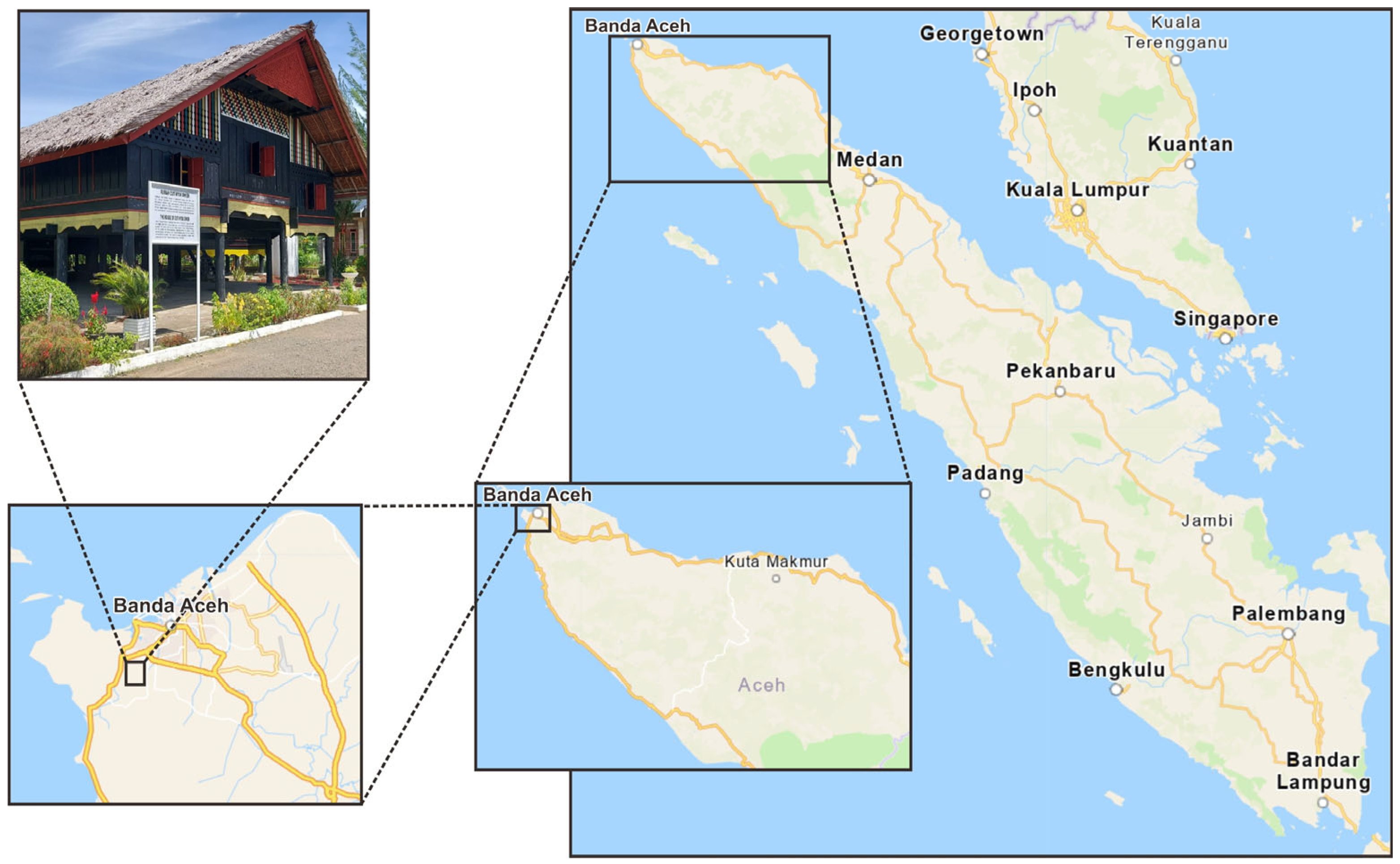By orienting the ventilation toward the prevailing wind direction, the building can help reduce indoor temperatures [22]. One example of a vernacular building is the Rumoh Aceh in Aceh Province, Indonesia [23,24].

Thermal performance in vernacular building plays a vital role in assessing how effectively these buildings can ensure a comfortable indoor environment. Air temperature, humidity, wind speed, and sunlight exposure significantly influence a building’s thermal behavior. Numerous studies have explored these aspects in vernacular structures across tropical regions. For instance, the study in [25] examined traditional Malay houses in Penang, Malaysia, and found that their well-designed natural ventilation systems resulted in lower indoor air temperature and humidity than outdoor conditions despite reduced indoor wind speed. Similarly, research in [26] evaluated the thermal characteristics of vernacular buildings in a hot and humid climate in Bushehr, Iran. It concluded that materials with low thermal conductivity like wood improved indoor thermal quality. Wood, known for its insulating properties, contributed to maintaining stable indoor temperatures. In another case, ref. [27] investigated traditional buildings in Yazd, Iran, and discovered that their thermal quality was relatively poor, requiring mechanical ventilation to enhance comfort. These findings underscore the importance of architectural design, choice of materials, and ventilation systems in shaping the thermal performance of vernacular buildings. Predictive thermal models are essential to better assess and improve thermal quality.

Thermal prediction models are designed to estimate indoor temperature conditions based on environmental factors and building attributes [28,29]. This model makes predictions to enhance occupant comfort, reduce energy consumption, and design more optimal ventilation and cooling systems, particularly in buildings [30,31]. Their primary function is to simulate and forecast indoor thermal behavior by analyzing various external variables and structural features. Generally, these models fall into two categories: physical models and data-driven models. Physical models rely on thermodynamic and heat transfer equations to replicate thermal conditions but require detailed architectural and thermal input data [32,33]. Although physical models are instrumental in the technical design of modern buildings, their application in the study of vernacular buildings is limited due to the requirement for detailed input variables [34]. Conversely, data-driven models utilize historical data to identify patterns between environmental parameters and indoor temperatures, offering greater flexibility and efficiency [35,36]. This model does not require detailed technical information about the building structure, making it easier to apply to traditional buildings with minimal architectural documentation [37]. Many studies have explored data-driven approaches to thermal prediction. For example, [38] used an Adaptive Neuro-Fuzzy Inference System (ANFIS) to predict air temperature in a livestock barn based on six days of environmental data, enabling optimized ventilation control for thermal stability and animal well-being. The model performance results show that the $RMSE$, $MAPE$, and $R^2$ values are 0.182, 0.548%, and 0.997, respectively. In paper [39], a Nonlinear Autoregressive with External Input (NARX) model was developed to forecast indoor temperatures in a commercial building, aiming to enhance energy efficiency without compromising thermal comfort. The statistical results show that the $MSE$ and $RMSE$ values are 0.083 and 0.837%, respectively. Additionally, [40] evaluated the effectiveness of various machine learning methods, such as Autoregressive Exogenous (ARX), Robust Multiple Linear Regression (RMLR), Extreme Learning Machine (ELM), Multilayer Perceptron (MLP), and NARX, combined with traditional approaches to predicting room temperatures in different parts of buildings. The study demonstrated that these predictive models support energy management and contribute to designing more thermally efficient and comfortable indoor environments. The numerical results indicate that the MLP-NARX method is the most accurate indoor temperature prediction, with an average annual $MAE$ of 0.111. This method outperforms the others due to its ability to capture nonlinear patterns and daily periodicity. The ARX method ranks second with an $MAE$ of 0.171, followed by RMLR at 0.207, MLP at 0.242, and ELM at 0.286. Consequently, developing data-driven thermal prediction models is a valuable strategy for optimizing building design and enhancing indoor thermal comfort.

Multiple Linear Regression (MLR) is a traditional statistical technique that models the linear relationship between a single dependent variable and multiple independent variables. MLR has been applied in thermal condition prediction, as demonstrated in [41], where an MLR model was developed to estimate indoor temperature in a mobile container using inputs such as global solar irradiance, ambient temperature, and wind speed. The model achieved relatively high accuracy, reporting an error rate of 7.1%. A key advantage of MLR is its strong interpretability; however, it struggles to capture nonlinear relationships. Artificial Neural Networks (ANNs) have been introduced to address this limitation, as they can learn complex, nonlinear patterns. A related study in [42] explored using ANN models to predict indoor thermal conditions, including air temperature, humidity, and wind speed, based on building orientation and geographical location. The results of this study indicate that the ANN-based predictive model produced error levels ranging from 0.03 to 1.05, demonstrating the effectiveness of this method in supporting building design oriented toward thermal comfort. Support Vector Regression (SVR), an extension of the Support Vector Machine (SVM) framework tailored for regression problems, has also been investigated in this context. SVR works by finding a predictive function that tolerates minor deviations and can handle nonlinear relationships using kernel functions. In paper [43], SVR was applied to predict air temperature inside a greenhouse. This approach aimed to address the complexity of the greenhouse temperature system, which is both nonlinear and time-varying. The study results show that the SVR model achieved the best performance, with a maximum relative error of 1.73%, an $MSE$ of 0.00019, and an $R^2$ of 0.99945. In comparison, the Backpropagation Neural Network (BPNN) model exhibited a higher error of up to 16.23%, an $MSE$ of 0.019564, and an $R^2$ of 0.96425. These findings confirm that the proposed SVR model is more accurate, stable, and effective in representing the actual temperature conditions in the greenhouse. Furthermore, the Generative Adversarial Network (GAN) is a data preprocessing technique capable of generating realistic data that closely resembles the original data, primarily imputing missing data. In paper [44], GAN was used to enhance the quality of mammographic images through data augmentation. By applying GAN, the dataset used for modeling became more representative. The results of this study demonstrate that applying GAN in the data preprocessing stage significantly enriches the dataset, thereby increasing the prediction model’s accuracy to 100%, compared to only 57.5% without augmentation. Paper [45] also highlights the critical role of GAN in data augmentation. The study used GAN to generate synthetic data to enrich the existing dataset. The study results indicate that applying GAN data augmentation improved the model’s accuracy from 76.1% to 88.5%. This approach not only successfully addressed data imbalance issues but also enhanced the generalization of the model. In addition, GAN offers advantages over simpler methods such as K-Nearest Neighbor (KNN) or mean substitution. In the mean substitution method, missing data is replaced with a fixed value, which can eliminate natural variability and alter the data distribution. Meanwhile, the KNN method tends to be less effective when dealing with high-dimensional data and requires considerable computational resources [46,47]. In contrast to these approaches, GAN can learn and understand the data distribution patterns more deeply through the adversarial mechanism between two networks: the generator and the discriminator. Through this competitive training process, GAN can generate synthetic data that closely resembles the original data, making it more effective in imputing missing data by the actual data distribution characteristics [48].

This study presents a hybrid method for developing an indoor temperature prediction model tailored to the traditional Rumoh Aceh building, using external environmental variables such as temperature, humidity, sunshine duration, and wind speed. The dataset combines ecological data sourced from the Meteorology, Climatology, and Geophysics Agency with sample measurements taken from four rooms within Rumoh Aceh structures located in Aceh Province, Indonesia. To ensure the dataset’s quality, a data preprocessing stage was conducted using the GAN method as an imputation technique to address the issue of missing data. This process generated synthetic data that closely resembled the original. Next, two primary predictive models, MLR and ANN, were applied, with each model further optimized using the SVR approach. The MLR algorithm was chosen due to its ease of interpreting regression coefficients. It allows the contribution of each variable to room temperature to be directly understood, although only for linear relationships. The ANN algorithm was then adopted to capture complex nonlinear patterns that MLR cannot address. Finally, the SVR approach was applied to reduce the risk of overfitting in models built from limited datasets. The MLR-SVR model combines the interpretability of MLR with the generalization capability of SVR. In contrast, the ANN-SVR model integrates the nonlinear modeling flexibility of ANN with SVR’s predictive precision. The evaluation used statistical metrics to determine the best-performing model with high accuracy, ensuring applicability in real-world conditions. The findings of this study present a practical approach for evaluating thermal performance in vernacular buildings and support architectural planning in designing more comfortable living environments. The main contributions of this paper are as follows:

• We propose a study to support passive thermal comfort in the Rumoh Aceh vernacular building by developing a predictive model to estimate indoor thermal conditions based on external environmental variables such as air temperature, humidity, sunshine duration, and wind speed.
• We introduce the GAN method in the data preprocessing stage to impute missing data, generating synthetic data that closely resembles the original. This technique enriches the dataset and improves model generalization.
• We propose two hybrid approaches: MLR optimized with SVR and ANN optimized with SVR. The goal is to compare model performance and determine the most accurate model for predicting indoor temperature in Rumoh Aceh based on external environmental parameters.

2. Materials and Methods

The simulation model developed in this study was designed using a computer with AMD Ryzen 5 4600H, 16 GB DDR4 RAM, and NVIDIA GeForce GTX 1650 Ti with 4 GB of memory. The software used included Python 3.10 with TensorFlow version 2.12.0, which was utilized for computation, analysis, and data visualization.

2.1. Data Acquisition

Rumoh Aceh is a vernacular building in the Aceh Province of Indonesia, characterized by its distinctive architecture designed to suit the region’s natural conditions and climate. These houses are built on raised platforms supported by wooden pillars, a structural approach that helps protect against flooding and enhances stability in earthquake-prone areas. The main framework is constructed using strong wood for durability. Key architectural features such as steeply sloped roofs and strategically placed ventilation openings support adequate airflow and help minimize indoor heat accumulation. The location of the Rumoh Aceh studied in this paper is in Banda Aceh, Indonesia, precisely at the coordinates 5°31′00.5″ N 95°16′18.1″ E, as shown in Figure 1. Meanwhile, Figure 2 presents a graph illustrating weather condition variations over the past three years in the study area.

This research incorporates meteorological data, including temperature, humidity, sunshine duration, and wind speed. The data were sourced from the Meteorology, Climatology, and Geophysics Agency of Aceh Province.

Table 1. Measuring instrument specifications.

Instrument	Sensor	Type	Range	Resolution	Accuracy
Environment	Temperature	HMP155	−80–60 °C	~0.01 °C	±0.5 °C
	Humidity	HMP155	0–100%	~0.1%	±2%
	Sunshine	CSD-3	400–1100 nm	-	±5%
	Wind Speed	Mi9000	2–60 m/s	~1.5 m/s	±0.5 m/s
Indoor	Temperature	DHT22	−40–80 °C	~0.1 °C	±0.5 °C

presents the specifications of the measuring instruments used. Data were recorded hourly throughout the day [49,50]. The probability distribution for each input parameter is assumed to follow a normal distribution. This assumption is based on the general characteristics of empirical data obtained from the Meteorology, Climatology, and Geophysics Agency over a long period. It is further supported by measurement data collected directly from four rooms in the Rumoh Aceh building.

Meanwhile, indoor air temperature measurements in the Rumoh Aceh building were carried out by the ASTM C-1046 standard [51]. Measurement device placement was strategically determined by analyzing heat flow directions to ensure that the data accurately reflected the building’s thermal environment. Each measurement location was required to exhibit one-dimensional heat flow to minimize errors from multidimensional heat transfer. Four rooms were selected for analysis: the lobby, a bedroom, and the left and right backrooms. Data collected from these areas served as representative samples for assessing the overall thermal distribution throughout the building. The layout for sensor placement is illustrated in Figure 3. The sensors were positioned in each corner of the rooms to achieve balanced data collection. They were placed away from ventilation openings to avoid interference from hot airflow that might compromise measurement accuracy [52,53]. Each sensor was mounted approximately 1.5 m above the floor, aligning with the typical human comfort zone. This positioning was chosen to ensure high-quality data by capturing evenly distributed heat, accurate thermal conditions, and dependable airflow measurements [54,55].

This paper’s modeling used six input variables and one output variable. This modeling aims to predict the indoor temperature in four different rooms. The input variables include minimum temperature ($T_{min}$), maximum temperature ($T_{max}$), average temperature ($T_{avg}$), average humidity ($H_{avg}$) from the surrounding environment, sunshine duration ($S_{time}$), and wind speed ($W_{speed}$). Meanwhile, the output variable is the indoor temperature ($T_{room}$) within each of the four rooms within the building. Further details regarding the input and output parameters are presented in

Table 2. Dataset parameters.

Parameter	Variable	Unit	Min	Max
Input	$T_{min}$	$℃$	21.6	24
	$T_{max}$	$℃$	30.6	35
	$T_{avg}$	$℃$	25.9	29.2
	$H_{avg}$	%	62	88
	$S_{time}$	$\mathrm{hour}$	2.5	10.4
	$W_{speed}$	${\displaystyle \raisebox{1ex}{$\mathrm{m}$}\!\left/ \!\raisebox{-1ex}{$\mathrm{s}$}\right.}$	4	13
Output	$T_{room}-1$	$℃$	24.9	33.1
	$T_{room}-2$	$℃$	24.6	33.8
	$T_{room}-3$	$℃$	25.3	33.1
	$T_{room}-4$	$℃$	24.1	32.9

.

2.2. Data Preprocessing

Data preprocessing is the initial stage in the data analysis and modeling process. One of the main challenges in this stage is missing data, which refers to incomplete entries in a dataset. Missing data can reduce model accuracy and performance if not properly handled [56,57]. One approach that can impute missing data is the Generative Adversarial Network (GAN) method, a machine learning architecture capable of generating missing estimates that closely resemble the original data distribution [58]. In the context of missing data reconstruction, the GAN modeling process begins by forming two neural network models: the generator ($G$) and the discriminator ($D$). The generator is responsible for producing estimates of the missing data based on the observed data, while the discriminator functions to distinguish between real data and imputed data. GAN is trained so that the generator produces data that is realistic enough to be indistinguishable from the original data. This process is carried out iteratively, where the generator and discriminator are trained simultaneously using the min-max optimization principle. Mathematically, the objective function of GAN is expressed as follows [59,60]:

$$\underset{G}{\mathit{min}}\underset{D}{\mathit{max}}V\left(D,G\right)={\mathbb{E}}_{x~p_{data}\left(x\right)}\left[\mathit{log}D\left(x\right)\right]+{\mathbb{E}}_{z~p_z\left(z\right)}\left[\mathit{log}\left(1-D\left(G\left(z\right)\right)\right)\right]$$

(1)

where $V\left(D,G\right)$ represents the value function that defines the training objective between the generator and discriminator, ${\mathbb{E}}_{x~p_{data}\left(x\right)}$ is the expectation over variable $x$ sampled from the original data distribution $p_{data}$ of the dataset, ${\mathbb{E}}_{z~p_z\left(z\right)}$ is the expectation over variable $z$ drawn from a random data distribution $p_z$ used as input to the generator, $G\left(z\right)$ denotes the synthetic data generated by the generator, and $D\left(x\right)$ represents the probability assigned by the discriminator. The generator’s input is not solely random data but rather a combination of observed data from the missing data entries and random noise $z$, resulting in an output $x_{recon}$ representing the fully reconstructed data. The discriminator then evaluates whether the obtained data originates from the original distribution or is generated through imputation. A reconstruction loss function is added to the objective function to ensure the training process effectively reconstructs missing data. This component measures how accurately the imputed data matches the original, expected values. The reconstruction loss function is formulated as follows [61]:

$${\mathcal{L}}_{recon}={\mathbb{E}}_{x_{true},x_{recon}}\left[{‖M⨀\left(x_{true}-x_{recon}\right)‖}^2\right]$$

(2)

where ${\mathbb{E}}_{x_{true},x_{recon}}$ denotes the expectation over all pairs of original data $x_{true}$ and imputed results $x_{recon}$, and $M$ represents the masking matrix that indicates the positions of the missing data elements. After the GAN training process and the model’s convergence, the generator can fill in the missing data entries with estimated values that follow the original data distribution.

2.3. Algorithm

This study introduces predictive models utilizing MLR and ANN optimized through SVR. These models are designed to forecast indoor temperature using available environmental parameters. The SVR-based optimization process aims to improve model performance by effectively capturing the relationship between input and output variables.

2.3.1. Multiple Regression Linear

MLR is a statistical technique that models the linear relationship between a single dependent variable and two or more independent variables. It expands upon simple linear regression, involving only one predictor variable [62]. The primary goal of MLR is to estimate the dependent variable using a linear combination of the independent variables while also assessing the individual impact of each predictor on the outcome [63,64]. MLR is widely applied across disciplines such as economics, engineering, social sciences, and environmental studies because it effectively accommodates multiple influencing factors in analyzing complex systems. The standard mathematical representation of the MLR model is given as follows [65]:

$$y=a_0+a_1{x}_1+a_2{x}_2+\cdots +a_n{x}_n+\epsilon$$

(3)

where $y$ denotes the dependent variable, while $x_1,x_2,\dots ,x_n$ represent the independent variables. The term $a_0$ is the intercept constant, and $a_1,a_2,\dots ,a_n$ are the regression coefficients that quantify the impact of each independent variable on the dependent variable. The error term $\epsilon$ accounts for the discrepancy between the actual value and the model’s predicted value. MLR aims to estimate the parameters $a_1,a_2,\dots ,a_n$ such that the difference between observed and predicted values is minimized. The most widely used technique for estimating these parameters is Ordinary Least Squares (OLS), which minimizes the Residual Sum of Squares (RSS), as defined below [65]:

$$\underset{a}{\mathit{min}}\sum _{i=0}^n{\left(y_i-a_0-\sum _{j=0}^n{a}_j{x}_{ij}\right)}^2$$

(4)

After determining the parameter values, the MLR model can be applied to estimate the dependent variable using new input values for the independent variables.

2.3.2. Artificial Neural Network

ANN is an approach in machine learning that mimics the way biological neural networks process information and make decisions. ANN is adaptive, as it can adjust weight values during training to learn complex input–output relationships, including nonlinear ones [66,67,68]. Each node receives inputs from the previous layer’s nodes in its computational process. These inputs are multiplied by their respective weights, summed up, and added to a bias term. The result of this operation, known as the weighted sum, is then passed through an activation function to produce the node’s output. This activation function is crucial in introducing nonlinearity into the network, allowing it to learn complex patterns. Mathematically, the output of a node can be formulated as follows [69,70]:

$$z=\sum _{i=1}^n{w}_i.x_i+b$$

(5)

$$y=f\left(z\right)$$

(6)

where $x_i$ denotes the input value at node $i$, $w_i$ is the weight associated with that input, $b$ is the bias term, and $f\left(z\right)$ is the activation function. In this paper, the activation function used is the ReLU (Rectified Linear Unit) function, which is defined as follows [71]:

$$f\left(z\right)=max\left(0,x\right)$$

(7)

The training of ANN focuses on determining the optimal weights and biases that minimize prediction errors. This begins with forward propagation, passing input data through the entire network to produce the predicted output. In the initial phase, the values of the hidden layer nodes are computed using the following equation [72]:

$$a^{\left(n\right)}=f\left(w^{\left(n\right)}.x+b^{\left(n\right)}\right)$$

(8)

where $x$ denotes the input node value and $a^{\left(n\right)}$, $w^{\left(n\right)},$ and $b^{\left(n\right)}$ represent the node values, weight matrix, and bias vector in the $n$ hidden layer, respectively. The node values in the output layer are then computed using the following equation [73]:

$$y=f\left(w^{(n+1)}.a^{\left(n\right)}+b^{(n+1)}\right)$$

(9)

where $y$ is the node value in the output layer. The generated output is then compared with the target or actual value using a loss function, which measures the network’s error. One of the most commonly used loss functions is the Mean Squared Error ($MSE$), which is formulated as follows [74]:

$$L={\displaystyle \frac{1}{n}}\sum _{i=1}^n{\left(y_i-{\widehat{y}}_i\right)}^2$$

(10)

where $n$ denotes the total number of data samples while $y_i$ and ${\widehat{y}}_i$ represent the network’s predicted output and the actual target value for the $i$ data point, respectively. This loss value is utilized in backpropagation, a calculus-based technique used to compute the partial derivatives of the loss function concerning each network weight [75]. The ANN can determine the optimal direction to adjust its parameters and progressively minimize prediction errors through this method. The network’s weights are subsequently updated using the gradient descent algorithm or its variants, which follow the negative gradient of the loss function. The gradient concerning the weight $w$ is calculated using the following equation [76]:

$${\displaystyle \frac{\partial L}{\partial w}}={\displaystyle \frac{\partial L}{\partial \widehat{y}}}.{\displaystyle \frac{\partial \widehat{y}}{\partial z}}.{\displaystyle \frac{\partial z}{\partial w}}$$

(11)

where ${\displaystyle \frac{\partial L}{\partial \widehat{y}}}$ represents the derivative of the loss function concerning the predicted output $\widehat{y}$, which simplifies to the expression $2\left(y_i-{\widehat{y}}_i\right)$. Next, ${\displaystyle \frac{\partial \widehat{y}}{\partial z}}$ refers to the derivative of the activation function, while ${\displaystyle \frac{\partial z}{\partial w}}$ denotes the derivative of the linear combination $z$ concerning the weight $w$. The updated weights are then computed using the following equation [76]:

$$w_{new}=w_{old}-\mu {\displaystyle \frac{\partial L}{\partial w}}$$

(12)

where $\mu$ denotes the learning rate, which determines the magnitude of each weight update step. The cycle of forward propagation, loss computation, backpropagation, and weight adjustment is iteratively performed across multiple epochs until the ANN reaches the target performance level.

2.3.3. Support Vector Regression

SVR is a variant of the SVM algorithm developed for regression tasks [77]. Unlike traditional linear regression, which minimizes the overall error between predicted and actual values, SVR seeks to identify a regression function that stays within a predefined margin of tolerance ($\epsilon$) from the target values while maintaining minimal model complexity. In other words, SVR attempts to construct a line that can predict the target values with a certain tolerance for error, ignoring minor errors as long as they are within the ε margin. This approach makes SVR a highly reliable method when dealing with nonlinear data and cases involving noise. In general, the SVR model seeks to find a regression function in the following form [78]:

$$f\left(x\right)=w^{T}x+b$$

(13)

where $w$ is the weight vector and $b$ is the bias. SVR aims to minimize the norm of the weight vector ${‖w‖}^2$ to prevent overfitting while ensuring that most of the training data lies within the deviation margin $\epsilon$. To accommodate data that cannot be predicted precisely within the $\epsilon$ margin, two relaxation variables, ${\xi }_i$ and ${\xi }_i^{\ast }$, are introduced, representing the positive and negative deviations from the margin boundary. The objective function to be minimized in SVR is expressed as follows [79]:

$$\underset{w,b,\xi ,{\xi }^{\ast }}{\mathit{min}}{\displaystyle \frac{1}{2}}{‖w‖}^2+C\sum _{i=1}^n\left({\xi }_i+{\xi }_i^{\ast }\right)$$

(14)

with subject

$$\left\{\begin{array}{c}{y}_i-f\left(x_i\right)\le \epsilon +{\xi }_i\\ f\left(x_i\right)-y_i\le \epsilon +{\xi }_i^{\ast }\\ {\xi }_i,{\xi }_i^{\ast }\ge 0\end{array}\right.$$

(15)

where $y_i$ denotes the actual target value, and $C$ represents the regularization parameter that balances the trade-off between the error tolerance outside the $\epsilon$-margin and the margin itself. A higher value of $C$ results in a stricter penalty for errors beyond the margin. To effectively model nonlinear relationships, SVR employs a kernel function that transforms the input data into a higher-dimensional space, enabling more precise linear regression. The regression function used in the SVR model is defined as follows [80]:

$$f\left(x\right)=\sum _{i=1}^n\left({\alpha }_i-{\alpha }_i^{\ast }\right)K\left(x_i,x\right)+b$$

(16)

where ${\alpha }_i$ and ${\alpha }_i^{\ast }$ represent the Lagrange multipliers derived from solving the dual optimization problem, while $K\left(x_i,x\right)$ denotes the kernel function, which manages nonlinear input–output relationships efficiently without explicitly transforming the data. In this study, the SVR model employs the Radial Basis Function (RBF) kernel, defined as follows [81]:

$$K\left(x_i,x\right)=e^{\left(-\gamma {‖x_i-x‖}^2\right)}$$

(17)

where $\gamma >0$ serves as a scaling parameter that determines how far the influence of each data point extends within the prediction function. The SVR model requires careful tuning of the parameters $C$, $\epsilon$, and kernel parameter $\gamma$ during training. After training, the SVR model predicts outputs for new inputs by leveraging the influence of the support vectors [82].

3. Modeling Process

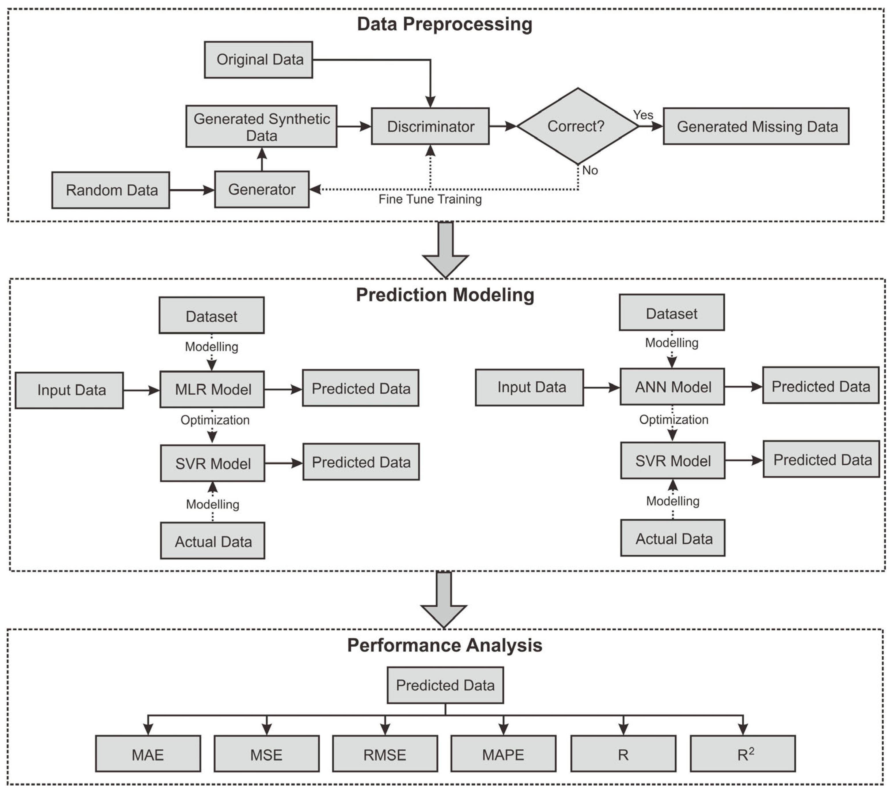
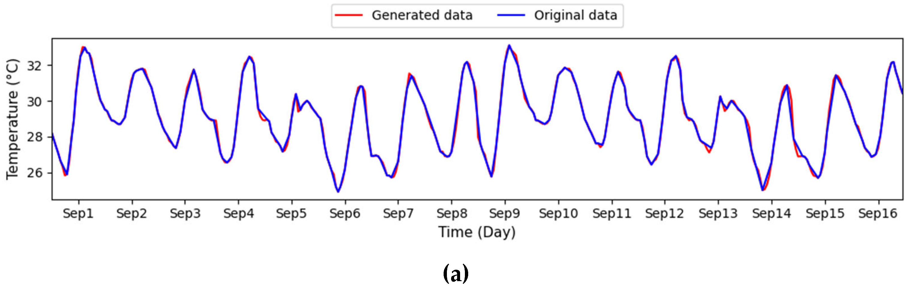
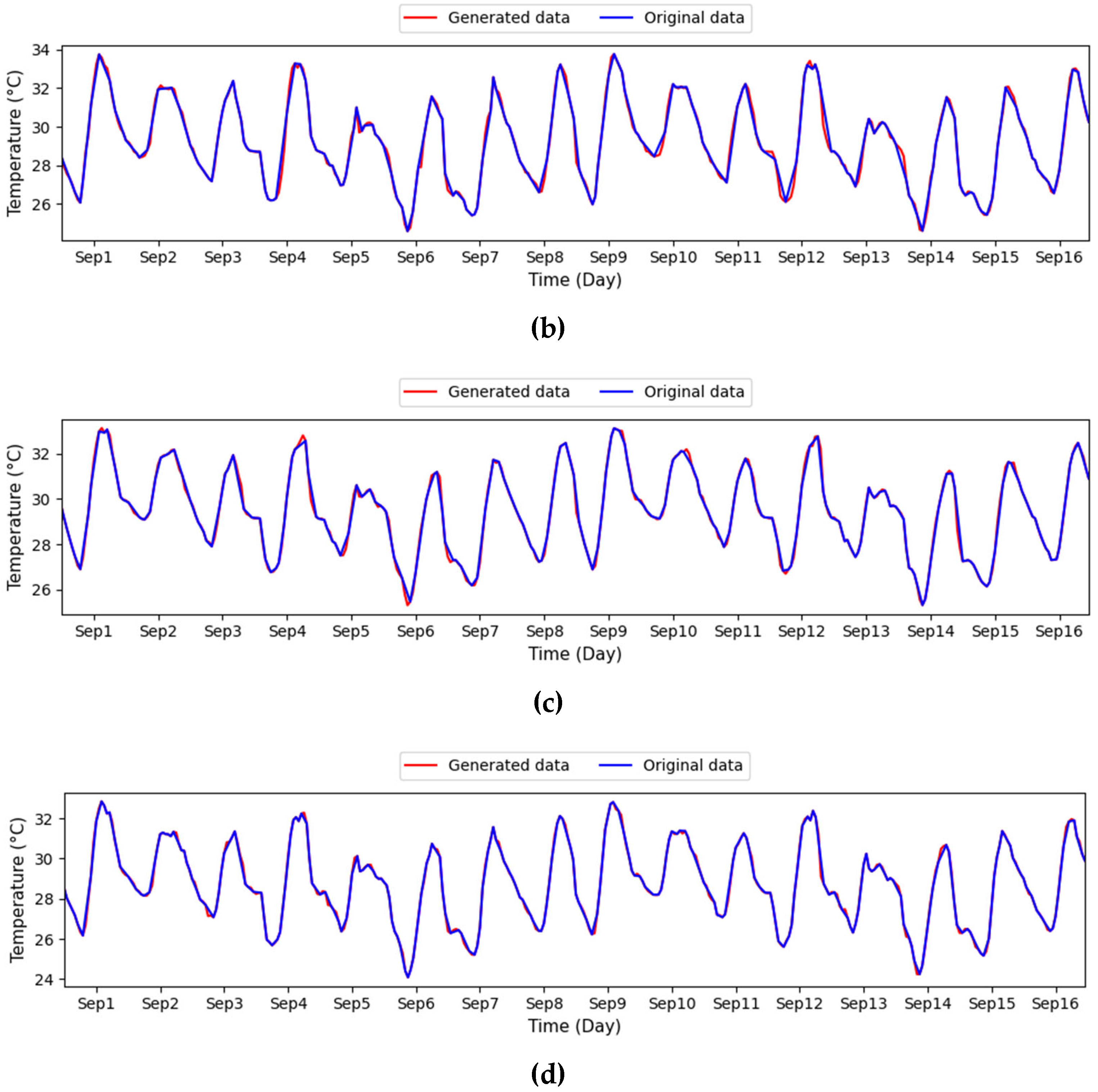
The modeling process in this study is divided into three stages: data preprocessing, prediction modeling, and performance analysis. For a clearer understanding of the predictive modeling methodology, the process diagram is presented in Figure 4. During the data preprocessing stage, a GAN-based method handles missing values within the dataset. The procedure involves inputting real and synthetic data produced by the generator into the discriminator. The GAN framework comprises two core components: the generator, which produces synthetic data resembling actual data, and the discriminator, which evaluates and differentiates between real and generated samples. By fine-tuning between the generator and the discriminator, the algorithm produces synthetic data deemed authentic by the discriminator. These data are then used to fill in the missing parts, resulting in a complete dataset. Next, the dataset is used in the prediction modeling stage, which comprises two models: MLR and ANN. The prediction results from each model are then optimized using an SVR approach. This technique allows the base models to provide an initial understanding of the data, which SVR further refines to improve prediction accuracy. The final stage is performance analysis, where the prediction results are evaluated using various statistical metrics. The evaluation involves an in-depth analysis of each model’s performance in predicting data and assessing the contribution of the GAN-based data imputation process to enhancing predictive model accuracy.

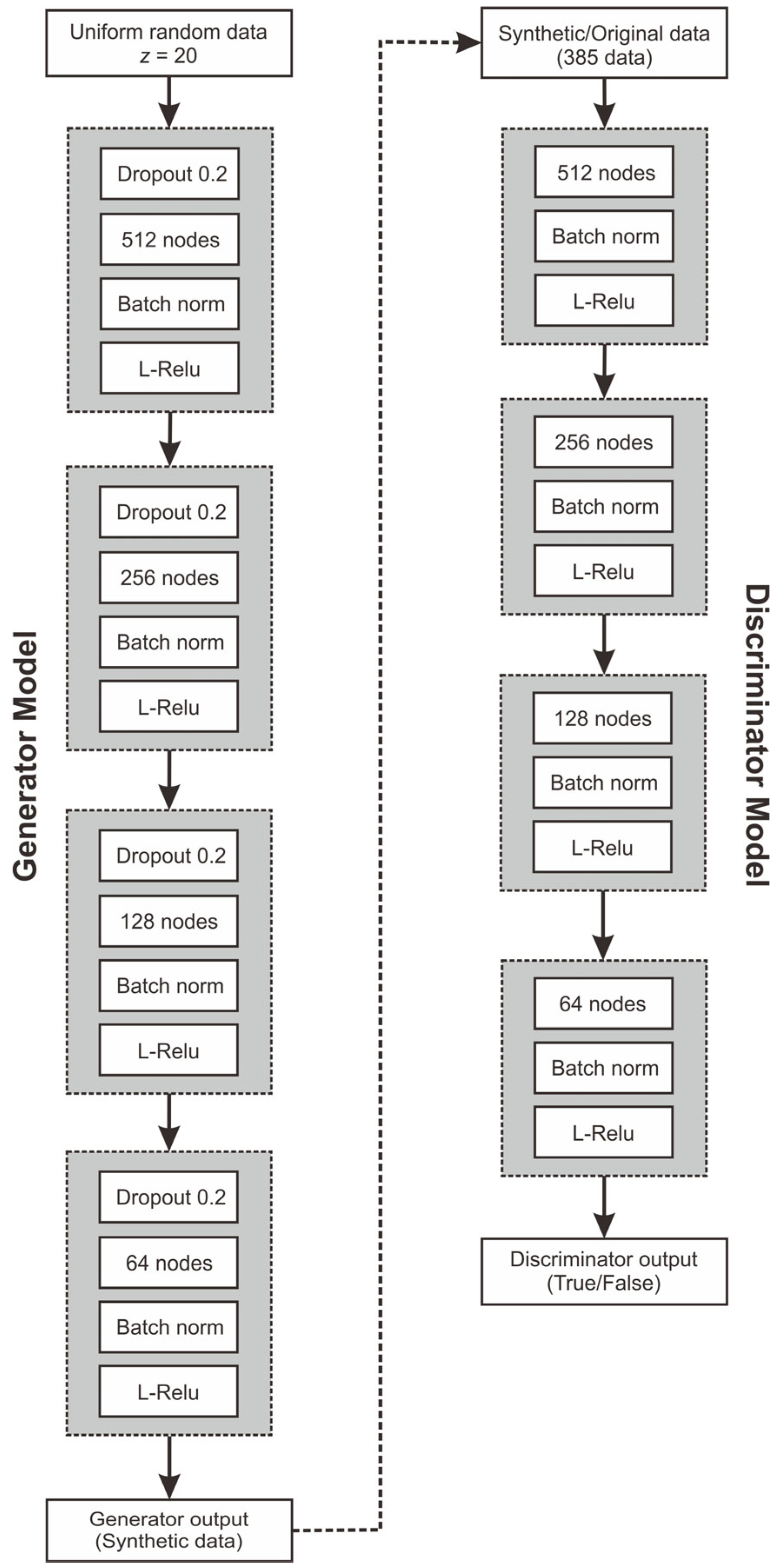
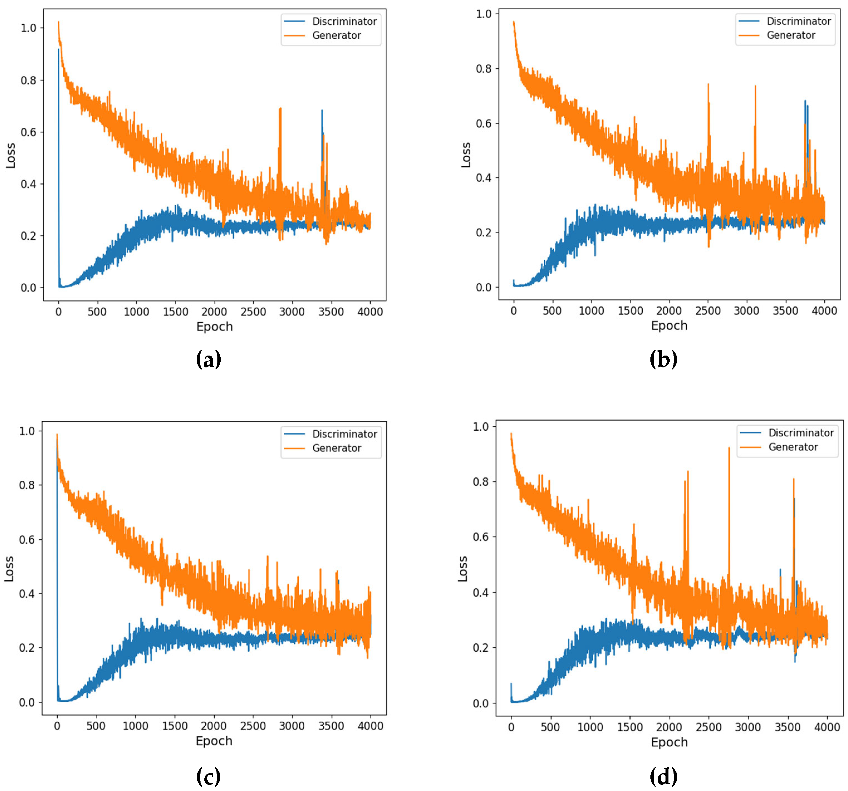
Figure 5 presents the architecture of the GAN, which is composed of two primary components: the generator and the discriminator. The generator takes a 20-dimensional random vector sampled from a uniform distribution and processes it through four layers. Each layer includes a combination of dropout, a defined number of nodes, batch normalization, and an activation function. The generator produces synthetic data to mimic real data fed into the discriminator. The discriminator’s role is to assess whether the input data is genuine or generated. It also features four sequential layers for processing. Training occurs in an adversarial manner: while the generator strives to create increasingly realistic data to fool the discriminator, the discriminator simultaneously enhances its ability to distinguish between real and synthetic inputs.

The structure of the MLR model with SVR optimization is shown in Figure 6. In this model, the initial approach uses MLR, which utilizes six input variables connected to one output room temperature variable through a series of coefficients from $a_0$ to $a_6$. Each input is multiplied by a specific coefficient and summed together with the common intercept ($a_0$) to generate the initial prediction data. The coefficient values for each room are presented in

Table 3. The constant coefficient values used in the MLR model.

Room	${\mathit{a}}_0$	${\mathit{a}}_1$	${\mathit{a}}_2$	${\mathit{a}}_3$	${\mathit{a}}_4$	${\mathit{a}}_5$	${\mathit{a}}_6$
1	22.8782	−0.2223	−0.0133	0.4488	−0.0065	0.0868	−0.0495
2	27.5445	−0.0992	0.0177	0.2019	−0.0343	0.1244	−0.0429
3	26.7997	−0.2302	−0.0035	0.3626	−0.0366	0.1773	−0.0165
4	14.9144	0.2016	0.1362	0.2366	−0.0252	0.0612	−0.0482

. Subsequently, the output from the MLR model is further optimized using the SVR approach, as illustrated on the right side of Figure 6. In this process, the output from the MLR model is used as input for SVR, which maps the input into a higher-dimensional space using a kernel function to minimize prediction error. Key parameters in SVR include the regularization constant ($C$), kernel parameter ($\gamma$), error margin ($\epsilon$), number of support vectors ($N_{SV}$), and bias value ($b$). These parameters are adjusted to obtain optimal values, producing more accurate prediction results. The parameter values for each room are shown in

Table 4. The parameter values used in the SVR model to optimize the MLR model.

Room	$\mathit{C}$	$\mathit{\gamma }$	$\mathit{\epsilon }$	${\mathit{N}}_{\mathit{S}\mathit{V}}$	$\mathit{b}$
1	100	0.1	0.05	22	29.7149
2	1000	0.05	0.05	23	31.0867
3	1000	0.05	0.05	20	30.7571
4	1000	0.01	0.05	21	30.6171

.

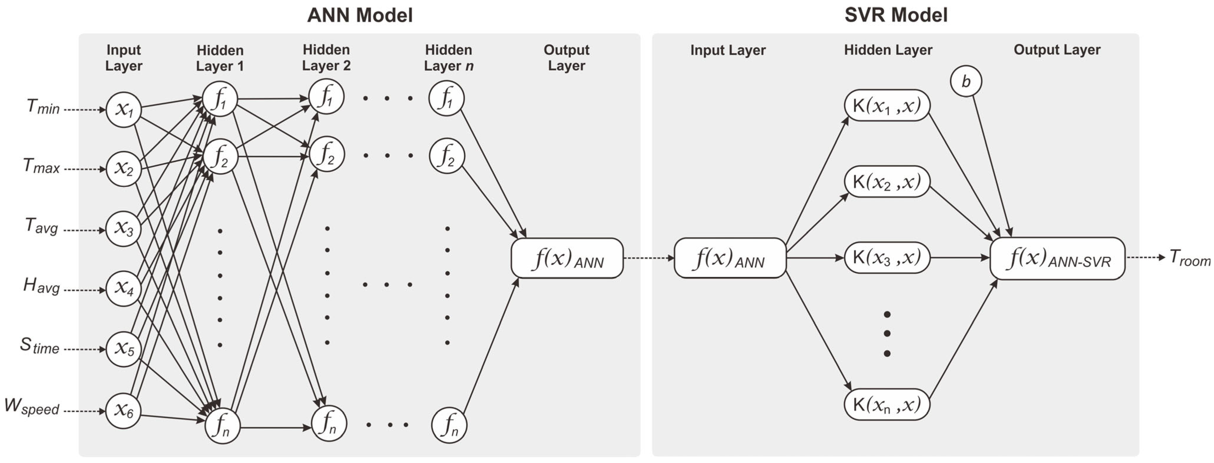
Meanwhile, Figure 7 displays the architecture of the ANN model refined through the SVR method. The model uses an artificial neural network to learn the nonlinear relationship between six input features and a single output. Its structure comprises four hidden layers, each containing a different number of neurons, and applies the ReLU activation function to enhance training efficiency.

Table 5. The structure of the ANN model.

Room	Feature	Value
1	Number of hidden layers	4
	Network structure	6–512–256–128–64–1
	Activation function	ReLU
	Learning rate	0.002
	Epoch	817
2	Number of hidden layers	4
	Network structure	6–512–256–128–64–1
	Activation function	ReLU
	Learning rate	0.001
	Epoch	1207
3	Number of hidden layers	4
	Network structure	6–512–256–128–64–1
	Activation function	ReLU
	Learning rate	0.001
	Epoch	1017
4	Number of hidden layers	4
	Network structure	6–512–256–128–64–1
	Activation function	ReLU
	Learning rate	0.001
	Epoch	1590

describes the network structure, including the number of layers, learning rate, and epochs adjusted for each room. After training, the ANN’s output is further refined using SVR. This step involves projecting the ANN predictions into a higher-dimensional space via a kernel function and determining the optimal hyperplane to boost prediction accuracy. The SVR parameters, shown in

Table 6. The parameter values used in the SVR model to optimize the ANN model.

Room	$\mathit{C}$	$\mathit{\gamma }$	$\mathit{\epsilon }$	${\mathit{N}}_{\mathit{S}\mathit{V}}$	$\mathit{b}$
1	100	0.1	0.05	15	28.1055
2	1000	0.1	0.05	18	28.8924
3	10	0.03	0.1	16	28.2237
4	10000	0.001	0.1	20	0.3554

, are specifically tuned to suit the unique characteristics of each room.

Several strategies were implemented in the model to prevent overfitting. First, the GAN architecture was equipped with dropout and batch normalization layers, preventing the model from relying too heavily on specific neurons. Second, an SVR approach was added to the model’s output. Third, setting the number of epochs and applying early stopping during ANN training helped halt the training process before the model began fitting into the datasets’ noise.

4. Performance Analysis Method

This study seeks to evaluate the performance of the proposed model through metric-based assessment and statistical analysis. The accuracy of the prediction model is measured using several standard metrics, including Mean Absolute Error ($MAE$), Mean Squared Error ($MSE$), Root Mean Squared Error ($RMSE$), and Mean Absolute Percentage Error ($MAPE$). $MAE$ calculates the average absolute difference between predicted and actual values, indicating the overall error magnitude. Both $MSE$ and $RMSE$ assess the expected, predicted, and actual variance outcomes. However, $RMSE$, the square root of $MSE$, is more responsive to larger errors, offering a deeper understanding of model accuracy. On the other hand, $MAPE$ represents prediction errors as a percentage of actual values, allowing for relative performance evaluation. The formulas for these metrics are presented below [83,84]:

$$MAE={\displaystyle \frac{1}{n}}\sum _{i=1}^n\left|y_i-{\widehat{y}}_i\right|$$

(18)

$$MSE={\displaystyle \frac{1}{n}}\sum _{i=1}^n{\left(y_i-{\widehat{y}}_i\right)}^2$$

(19)

$$RMSE=\sqrt{{\displaystyle \frac{1}{n}}\sum _{i=1}^n{\left(y_i-{\widehat{y}}_i\right)}^2}$$

(20)

$$MAPE={\displaystyle \frac{1}{n}}\sum _{i=1}^n\left|{\displaystyle \frac{y_i-{\widehat{y}}_i}{y_i}}\right|.100\%$$

(21)

where $n$ denotes the total number of test data points, while $y_i$ and ${\widehat{y}}_i$ represent the actual and predicted values for the $i$ data point, respectively. In addition to the error metrics, statistical indicators such as the correlation coefficient ($R$) and the coefficient of determination ($R^2$) are employed. The correlation coefficient $R$ measures the strength and direction of the linear relationship between two variables. An $R$ value close to 1 suggests a strong positive correlation, meaning both variables tend to increase or decrease together. Conversely, an $R$ value near −1 signifies a strong negative correlation, where an increase in one variable corresponds with a decrease in the other. An $R$ value close to 0 implies a weak or negligible linear relationship. The coefficient of determination $R^2$ evaluates the regression model’s performance by quantifying the proportion of variance in the dependent variable that the model can explain. The $R^2$ ranges from 0 to 1, where 0 indicates no explanatory power, and 1 indicates that the model accounts for all observed variance. The corresponding equations for these statistical indicators are provided below [85]:

$$R={\displaystyle \frac{n{\sum }_{i=1}^n{y}_i{\widehat{y}}_i-\left({\sum }_{i=1}^n{y}_i\right)\left({\sum }_{i=1}^n{\widehat{y}}_i\right)}{\sqrt{\left[n\sum _{i=1}^n{y}_i^2-{\left(\sum _{i=1}^n{y}_i\right)}^2\right]\left[n\sum _{i=1}^n{\widehat{y}}_i^2-{\left(\sum _{i=1}^n{\widehat{y}}_i\right)}^2\right]}}}$$

(22)

$$R^2=1-{\displaystyle \frac{{\sum }_{i=1}^n{\left(y_i-{\widehat{y}}_i\right)}^2}{{\sum }_{i=1}^n{\left(y_i-\overline{y}\right)}^2}}$$

(23)

Uncertainty analysis using the Monte Carlo method is a statistical technique used to estimate the uncertainty of a system or model’s output by randomly simulating input variations based on known probability distributions. This analysis is conducted by defining a distribution for each input, followed by Monte Carlo sampling, which is expressed as follows [86]:

$$\overline{{\widehat{T}}_i}={\displaystyle \frac{1}{M}}\sum _{k=1}^M{\widehat{T}}_i^{\left(k\right)}$$

(24)

where $\overline{{\widehat{T}}_i}$ is the average prediction obtained from all samples, $M$ is the number of Monte Carlo samples, and ${\widehat{T}}_i^{\left(k\right)}$ is the predicted value using the $k$ sample at data point $i$. From all the generated predictions, the standard deviation of the output (${\sigma }_{input,i}$) is calculated using the following equation [87]:

$${\sigma }_{input,i}=\sqrt{{\displaystyle \frac{1}{M-1}}\sum _{k=1}^M{\left({\widehat{T}}_i^{\left(k\right)}-\overline{{\widehat{T}}_i}\right)}^2}$$

(25)

Then, the mean value is calculated using the following equation [88]:

$$\overline{{\sigma }_{input}}={\displaystyle \frac{1}{N}}\sum _{i=1}^N{\sigma }_{input,i}$$

(26)

There are two components of uncertainty: the standard deviation of the model prediction error (${\sigma }_{model}$), which is measured using $RMSE$, and the standard deviation of the prediction resulting from input variability (${\sigma }_{input}$). These two components are assumed to be independent, as $RMSE$ originates from the inherent error of the model, while ${\sigma }_{input}$ arises from measurement noise in the input. Therefore, the total prediction uncertainty can be calculated using the following equation [89]:

$${\sigma }_{total}=\sqrt{{\left(\overline{{\sigma }_{input}}\right)}^2+{\left({\sigma }_{model}\right)}^2}$$

(27)

If the output distribution approximates a normal distribution, the 95% confidence interval can be expressed as $\pm 1.96{\sigma }_{total}$.

5. Results and Discussion

This section presents a performance evaluation for each room and an assessment of the model’s overall effectiveness. The review involves several stages, including data preprocessing, model training, testing, and comparative analysis. The model was trained on a dataset comprising 385 records in this study. The model was validated by splitting the dataset into 80% training and 20% testing data, then evaluating its performance using statistical metrics such as $MAE$, $MSE$, $RMSE$, $MAPE$, $R$, and $R^2$ for each room. In addition, the quality of GAN imputation was assessed through the loss curve during training to ensure convergence and the ability to replicate the original data distribution. Further error analysis was conducted by comparing predicted and actual values on the test data to identify how well the model captures thermal patterns and the extent of deviation. Uncertainty analysis was also performed to assess the sensitivity level of the proposed model.

5.1. Data Preprocessing Results

Figure 8 depicts the loss trends observed during the GAN model’s training across four rooms. The graphs show that the generator initially exhibits a high loss, which gradually declines with increasing epochs. This trend indicates that the generator’s ability to produce data that resembles real data is improving. In contrast, the discriminator’s loss typically increases during the early training stages before stabilizing, suggesting it becomes more effective at distinguishing real data from generated data as the generator’s output quality improves. Minor fluctuations in both losses reflect the adversarial nature of the GAN training process. The consistent patterns across all four rooms demonstrate the model’s stable and reliable training behavior under varying environmental conditions.

Figure 9 presents the results of the missing data imputation. After the imputation process, a more complete dataset that closely resembles the original data pattern was obtained. The imputed data successfully follows the trend of the original data. This alignment demonstrates that the GAN model can learn the temporal characteristics of temperature data and generate accurate estimated values.

5.2. Performance Analysis of Prediction Models

Figure 10 presents a comparison of prediction errors across different rooms. Each plot displays the error values for 30 data indices, comparing four models. In general, the errors for each model fall within a relatively narrow range, between −2 and 2, indicating that all four models demonstrate fairly good prediction performance. The error variation remains relatively high in Room 1 and Room 2, especially in the MLR and MLR-SVR models, which exhibit a wider spread of errors than the ANN model. In contrast, Room 3 and Room 4 show errors more concentrated around zero, indicating more accurate and stable predictions, particularly in the ANN and ANN-SVR models. This pattern suggests that ANN-based models produce more precise results, especially when combined with nonlinear regression techniques such as SVR. Overall, the ANN-SVR model consistently delivers the best performance across all four rooms based on the distribution of error values.

Figure 11 compares actual and predicted temperatures from four different models. The closer the data points are to the reference line, the better the model’s performance in predicting the temperature. In Rooms 1 and 2, the data points from the ANN and ANN-SVR models appear more concentrated around the reference line than in the MLR and MLR-SVR models. The same pattern is observed in Room 3 and Room 4, where the ANN-SVR model consistently produces results closer to the actual temperature. On the other hand, the MLR model tends to show a wider spread from the reference line, indicating that the linear regression method is less capable of capturing the data’s complexity. Therefore, it can be concluded that the ANN-SVR model performs the best in predicting room temperatures with high precision across all four rooms tested.

Based on the performance evaluation results summarized in

Table 7. The performance evaluation of each model.

Room	Model	$\mathit{M}\mathit{A}\mathit{E}$	$\mathit{M}\mathit{S}\mathit{E}$	$\mathit{R}\mathit{M}\mathit{S}\mathit{E}$	$\mathit{M}\mathit{A}\mathit{P}\mathit{E}$	$\mathit{R}$	${\mathit{R}}^2$
1	MLR	0.235	0.082	0.286	0.793%	0.789	0.622
	MLR-SVR	0.196	0.056	0.237	0.661%	0.723	0.523
	ANN	0.164	0.057	0.238	0.562%	0.667	0.445
	ANN-SVR	0.075	0.016	0.125	0.256%	0.699	0.489
2	MLR	0.278	0.118	0.344	0.948%	0.63	0.397
	MLR-SVR	0.105	0.025	0.157	0.356%	0.593	0.351
	ANN	0.176	0.068	0.26	0.56%	0.879	0.773
	ANN-SVR	0.152	0.046	0.214	0.516%	0.844	0.712
3	MLR	0.2	0.063	0.251	0.67%	0.9	0.81
	MLR-SVR	0.205	0.067	0.259	0.686%	0.87	0.757
	ANN	0.324	0.161	0.4	1.094%	0.815	0.664
	ANN-SVR	0.279	0.114	0.338	0.938%	0.814	0.662
4	MLR	0.219	0.079	0.28	0.762%	0.819	0.671
	MLR-SVR	0.176	0.053	0.229	0.609%	0.811	0.657
	ANN	0.25	0.096	0.31	0.871%	0.801	0.641
	ANN-SVR	0.148	0.037	0.193	0.515%	0.781	0.61

, the ANN-SVR model demonstrates the highest overall accuracy. In Room 1, it achieved the lowest error values, $MAE$ of 0.117, $RMSE$ of 0.087, and $MAPE$ of 0.258, along with the highest correlation and determination coefficients, with $R$ and $R^2$ values of 0.986 and 0.936, respectively. A similar pattern is evident in Room 2, where the ANN-SVR model again outperforms the others, achieving an $MAE$ of 0.052 and $R^2$ of 0.971. These results surpass those of the other models, which generally produce higher error values and lower $R^2$ scores. In Room 3, although the SVR model records a slightly higher $R$ value than the ANN-SVR model, the latter significantly reduces error metrics, confirming its superior predictive performance. In Room 4, the standalone ANN model shows marginally better $R$ and $R^2$ values. However, the ANN-SVR model yields the lowest $MAE$, $RMSE$, and $MAPE$, indicating better error minimization. Overall, the ANN-SVR model consistently delivers the most accurate temperature predictions across all four rooms in the Rumoh Aceh building, making it the most effective model for this application.

The analysis also shows that the $R^2$ values cannot fully explain the temperature variations in some rooms, particularly where $R^2$ is below 0.8. This condition indicates that important variables are still not yet included in the model. Several steps can be taken to improve the $R^2$ values, including incorporating internal factors such as the type and thermal properties of building materials, the building’s orientation to the sun, and ventilation conditions, which significantly influence the thermal dynamics inside the building. In addition, increasing the size of the dataset is also necessary to enhance the model’s generalization capability.

Table 8. The uncertainty analysis results.

Room	$\overline{{\mathit{\sigma }}_{\mathit{i}\mathit{n}\mathit{p}\mathit{u}\mathit{t}}}$ (°C)	${\mathit{\sigma }}_{\mathit{m}\mathit{o}\mathit{d}\mathit{e}\mathit{l}}$ (°C)	${\mathit{\sigma }}_{\mathit{t}\mathit{o}\mathit{t}\mathit{a}\mathit{l}}$ (°C)	$95\mathit{\%}\mathbf{C}\mathbf{I}(\pm 1.96{\mathit{\sigma }}_{\mathit{t}\mathit{o}\mathit{t}\mathit{a}\mathit{l}})$
1	0.11	0.125	0.17	±0.33 °C
2	0.47	0.214	0.52	±1.02 °C
3	0.39	0.338	0.52	±1.02 °C
4	0.36	0.193	0.41	±0.8 °C

presents the uncertainty analysis results using the Monte Carlo method for the ANN-SVR model in predicting room temperature. The Monte Carlo iterations were conducted over 1000 epochs. The study shows that Room 1 has a relatively low uncertainty, with a confidence interval of ±0.33 °C. Meanwhile, Room 2 and Room 3 exhibit the same confidence interval of ±1.02 °C, although with different standard deviation compositions. This indicates that the contribution of each source of uncertainty may vary yet still result in a similar level of total uncertainty. For these two rooms, the confidence interval reaches ±1.02 °C. As for Room 4, the confidence interval is ±0.8 °C. Although the confidence interval values in Room 2 and Room 3 are relatively high, at ±1.02 °C, the ANN-SVR model still demonstrates statistically accurate predictive performance, as shown in Table 7. Furthermore, according to ASHRAE 55 Standard, temperature fluctuations should not exceed ±1.1 °C within 15 min or ±2.2 °C within 1 h [90]. Therefore, the uncertainty of ±1.02 °C remains within the permissible range of temperature variation dynamics, although it does not directly represent the level of thermal comfort. In addition, thermal comfort is not solely determined by the physical parameters of the environment but is also significantly influenced by individual psychological factors [91]. These psychological factors refer to a person’s perception of adjusting to thermal conditions based on experience, expectations, personal preferences, and social and cultural conditions [92].

As a form of validation for the proposed ANN-SVR model, a performance comparison was conducted with several models from previous highly relevant studies. The comparison results presented in

Table 9. The comparison of the proposed model with other published models.

Model	$\overline{\mathit{M}\mathit{A}\mathit{E}}$	$\overline{\mathit{M}\mathit{S}\mathit{E}}$	$\overline{\mathit{R}\mathit{M}\mathit{S}\mathit{E}}$	$\overline{\mathit{M}\mathit{A}\mathit{P}\mathit{E}}$	$\overline{\mathit{R}}$	$\overline{{\mathit{R}}^2}$
NARX [39]	-	0.083	-	0.837%	-	-
ANFIS [38]	-	-	0.677	2.529%	-	0.743
BPNN [43]	-	0.01956	-	-	-	0.99945
PB-MLR [33]	34,113	-	52,232	2.64%	-	0.9784
XGBoost [93]	1.2088	1.5782	1.2562	-	-	0.8312
PSO-XGBoost [93]	0.1495	0.0281	0.1676	-	-	0.9969
ANN-SVR (Proposed)	0.164	0.053	0.218	0.556%	0.785	0.618

show that the ANN-SVR model developed in this study outperforms all the benchmark models. This reinforces the conclusion that the proposed combination of ANN and SVR provides high accuracy and is suitable for being considered a reliable predictive model.

5.3. Thermal Prediction Results

Based on the ANN-SVR model, which has proven to be the most optimal predictive model, the process of predicting room temperature based on variations in environmental parameters was carried out. Figure 12a shows that the expected temperature increases as the outdoor temperature rises, with Room 3 showing the highest predicted temperature compared to the other rooms. This indicates that the outdoor temperature significantly impacts the indoor temperature, especially in Room 3. Figure 12b shows that an increase in outdoor humidity tends to lower the predicted temperature in all four rooms, indicating a negative influence of humidity on the room temperature. However, Room 3 still maintains the highest predicted temperature. Next, in Figure 12c, it is shown that the longer the duration of sunlight, the higher the room temperature, especially in Room 3 and Room 2. This suggests that solar radiation plays a significant role in increasing the room temperature. Finally, Figure 12d shows that wind speed does not have as significant an effect as the other variables. However, there is a slight trend of temperature increase with the increasing wind speed, particularly in Room 3 and Room 1. Overall, the prediction results indicate that the ANN-SVR model is quite sensitive to changes in environmental condition parameters, with Room 3 consistently showing higher predicted temperatures in nearly all conditions. This is due to the absence of direct ventilation to the outside environment in that room, causing hot air to be trapped and accumulated inside. Meanwhile, variations in solar intensity were not tested because solar intensity is highly sensitive to microclimatic conditions and environmental obstructions, such as surrounding trees or buildings. As a result, it does not always accurately represent the overall level of solar exposure the building receives.

The developed model is general and can be applied to other vernacular buildings in tropical regions. However, to apply it to buildings with different architectural characteristics, the model needs to be retrained using appropriate local data to capture the specific influences of the local climate.

6. Conclusions

Based on the evaluation results, applying the GAN method has proven effective in addressing missing data issues and can enhance the overall quality of the dataset. On the other hand, the ANN-SVR predictive model demonstrated the most optimal performance in terms of accuracy and stability. Evaluation results show that this model achieved the lowest average $\overline{MAE}$ and $\overline{RMSE}$ values, at 0.164 and 0.218, respectively, and the highest average $\overline{R}$ and $\overline{R^2}$ values, at 0.785 and 0.618, respectively. This performance surpasses the MLR, MLR-SVR, and conventional ANN models. The predictive analysis results also show that environmental temperature and solar radiation duration are the dominant factors contributing to the increase in room temperature. At the same time, humidity has a negative influence, and wind speed has a relatively minor impact. These findings emphasize the effectiveness of integrating the GAN method in the preprocessing stage with the ANN-SVR predictive model while also serving as a reference for planners and architects to improve thermal comfort in vernacular buildings such as the Rumoh Aceh. However, the model developed in this study still does not consider internal factors such as occupant behaviour, building materials, and the available ventilation system. This may result in prediction outcomes that do not fully reflect the actual conditions. In practice, these factors significantly impact the thermal dynamics within the building, so the obtained predictions still do not fully represent the thermal conditions in an absolute sense. However, this model still demonstrates high accuracy based on variations in external environmental conditions and can serve as a foundation for further development by incorporating internal factors. Therefore, additional research can be conducted to develop a model that dynamically adapts based on changes in environmental conditions, occupant activity, building materials, and available ventilation. This makes the results more applicable in supporting the design planning of vernacular buildings with high thermal quality. In addition, this study has not explicitly addressed the psychological aspects of occupants in evaluating thermal comfort. By incorporating these psychological factors, further research can better understand thermal conditions in vernacular buildings.