A Rapid Sand Gradation Detection Method Based on Dual-Camera Fusion

Abstract

Precise grading of manufactured sand is vital to concrete performance, yet standard sieve tests, though accurate, are too slow for online quality control. Thus, we devised an image-based inspection method combining a dual-camera module with a Temporal Interval Sampling Strategy (TISS) to enhance throughput while maintaining precision. In this design, a global wide-angle camera captures the entire particle field, whereas a local high-magnification camera focuses on fine fractions. TISS selects only statistically representative frames, effectively eliminating redundant data. A lightweight segmentation algorithm based on geometric rules cleanly separates overlapping particles and assigns size classes using a normal-distribution classifier. In tests on ten 500 g batches of manufactured sand spanning fine, medium, and coarse gradations, the system processed each batch in an average of 7.8 min using only 34 image groups. It kept the total gradation error within 12% and the fineness-modulus deviation within ±0.06 compared to reference sieving. These results demonstrate that the combination of complementary optics and targeted sampling can provide a scalable, real-time solution.

1. Introduction

The particle-size gradation of manufactured sand (fine aggregate) is a key indicator of aggregate quality. It governs the packing structure and stress-transfer pathways in concrete, thereby affecting workability, mechanical performance, and durability [1,2]. As construction standards rise and schedules tighten, the industry urgently requires rapid, fully automated gradation measurement to replace labour-intensive manual methods [3].

Two mainstream approaches are currently used. Traditional sieve analysis is standardised and accurate, but it relies on manual work, lacks repeatability, and cannot support continuous online monitoring [4,5]. Image-based techniques offer non-contact operation and high levels of automation, making them an attractive alternative [6]. However, existing systems rarely meet industrial efficiency demands. A 500 g sample of manufactured sand contains millions of particles between 0.075 mm and 4.75 mm, the size range defined for construction sand in Chinese national standards [7,8]. This classification, though different from some international standards [9,10], reflects common engineering practice in China.

When pixel density is increased to detect particles smaller than 0.3 mm, the field of view narrows so much that thousands of images are needed to cover one sample. Enlarging the field of view retains coverage but sacrifices resolution, making fine particles hard to detect. This hardware trade-off leads to image acquisition and processing times that often exceed production control requirements [11].

The present study tackles this bottleneck by reducing both the number of images captured and the processing burden, without compromising accuracy. The proposed solution introduces three principal innovations:

• Dual-camera architecture with temporal-interval sampling: This design pairs a wide-angle global camera with a high-magnification local camera, selecting only statistically representative frames. The approach significantly enhances acquisition efficiency without compromising coverage or detail.
• Adaptive segmentation with statistical classification: An adaptive segmentation algorithm for bonded particles is integrated with a statistical size-classification model. This ensures stable detection accuracy, even under sparse sampling conditions.
• Comprehensive performance evaluation: Experiments on ten 500 g batches covering fine, medium, and coarse gradations showed an average detection cycle of 7.8 min per batch. The total gradation error remained below 12%, and fineness-modulus deviation remained within ±0.06, confirming the method’s suitability for scalable, real-time industrial deployment.

2. Related Work

Given the broad size range and high packing density of fine aggregates, recent research has aimed to improve all stages of image-based gradation detection, including camera design, particle segmentation, and size analysis. The accuracy and adaptability of image capture ultimately constrain the performance of downstream processing. To address fluctuating illumination and complex particle piles under field conditions, many tailored imaging schemes have been developed.

Li et al. [12] created a digital acquisition system with adjustable lighting and resolution that permits real-time monitoring on construction sites, thereby boosting both speed and robustness. Huang et al. [13] devised a falling-particle platform that enhances image quality through grayscale conversion and filtering, yet its camera cannot resolve particles finer than 0.15 mm. Lin et al. [14] addressed this gap with a dual-camera, multiscale setup designed to recover missing fine fractions, whereas Zhao et al. [15] took a different approach by using three cameras to view rotating aggregates from multiple angles and building a 2D image library to mitigate dynamic imaging errors. However, even with such setups, dynamic acquisition demands high-speed shutters and precise lighting synchronisation, and ultra-fine grains tend to disperse during motion. These factors impair data stability. To avoid the challenges of dynamic imaging, Zhang et al. [16] adopted a static local sampling approach. Multiple close-up shots provided reliable fine-particle estimates, but repeated sampling greatly slowed the workflow and failed to meet real-time, high-throughput demands.

Because sand particles naturally clump and overlap, inadequate segmentation directly degrades size measurements. Classical segmentation methods—for example, the threshold-plus-watershed routine proposed by Leonardo et al.  [17] and the wavelet-based variant introduced by Zhang et al. [18]—can split some adhered grains in static images. However, these approaches rely on manually tuned thresholds and are prone to both over-segmentation and under-segmentation. In recent years, deep learning has been explored as an alternative solution. Zhu et al. [19] built a two-stage FCN that first detects targets, then separates contacts; Cao et al. [20] proposed Multi-ResUNet, which inserts Inception blocks and residual links to handle severe occlusion; and Yang et al. [21] applied Mask R-CNN augmented with generative adversarial network (GAN)-generated data to improve generalisation. Despite their higher accuracy, these deep models still struggle with densely adhered particles and are sensitive to scene changes. They also require large labeled datasets and long training cycles, making industrial deployment difficult.

Another challenge is converting two-dimensional image data into accurate gradation estimates. Many studies have tried to translate 2D particle contours into gradation proxies. For instance, Kumara et al. [22] recommended using the Feret diameter for irregular particle shapes, Liu et al. [23] added an aspect-ratio metric to reflect particle flatness, Zhou et al. [24] paired the projected area with the Feret diameter to estimate particle volume, and Xu et al. [25] introduced a correction factor to reduce bias in volume estimates from 2D images. However, any purely 2D projection misses the particle thickness, so errors persist. Therefore, researchers have explored 3D approaches: Liang et al. [26] used laser scanning to capture particle shapes, and Su et al. [27] employed micro-focus X-ray computed tomography (CT) to reconstruct high-fidelity 3D models. However, both techniques require expensive equipment and intensive computation, which limits their on-site practicality.

Deep learning has also been applied to particle classification and overall gradation prediction. Siyao et al. [28] enhanced the U-Net architecture with multi-scale fusion and a custom loss function for this task. Li et al. [29] used transfer learning to train a ResNet50 classifier on sand images. Chen et al. [30] fitted a nonlinear mapping between image-derived gradations and true gradations for dynamic calibration. Buscombe’s SediNet [31] performs end-to-end gradation prediction, while Kim et al. [32] used synthetic data with transfer learning to compensate for limited training samples. Li and Iskander [33] achieved accurate particle sorting through conventional supervised learning on hand-crafted image descriptors. Although these data-driven models excel in accuracy, they depend on large, well-annotated datasets and long training cycles, which complicates their deployment. As a result, they are not yet well suited for real-time industrial monitoring.

In short, image-based gradation analysis has made substantial progress, yet the full pipeline still struggles to balance speed and precision. This study addresses this challenge by integrating dual-view collaborative imaging, multiscale region fusion, and a weighted error-correction framework. This combination stabilises fine-fraction detection without the need for extreme image resolution, achieving high accuracy while significantly improving efficiency and facilitating on-site deployment.

3. Methodology

This study presents a high-throughput image analysis pipeline for manufactured sand gradation that addresses the twin challenges of fine-particle resolution and data capture speed. The hardware integrates quantitative feeding, vibration-assisted dispersion, synchronised dual-camera imaging, and pneumatic sand cleaning within a closed-loop automated platform. A Temporal Interval Sampling Strategy (TISS) accelerates acquisition without compromising representativeness. On the software side, multi-frame fusion background subtraction and block-wise adaptive thresholding feed into a Recursive Concavity-Guided Segmentation (RCGS) algorithm, which effectively separates adhered grains and generates reliable particle contours. Gradation is computed by combining a normal-distribution size classifier with a volume estimator based on Feret diameter and projected area. Finally, a dual-view fusion module reconciles global and local data through normalisation and weighted error correction, delivering accurate overall gradation. Together, these innovations enhance both precision and throughput, offering a practical solution for real-time fine-aggregate quality monitoring in industrial settings.

3.1. Image Acquisition Optimization

Traditional image-based detection systems often suffer from low cleaning efficiency, uneven sample coverage, limited fine-particle visibility, and long processing times. To address these challenges, we implemented systematic optimisations in both hardware and sampling strategy. The closed-loop detection platform now integrates quantitative feeding, vibration-assisted dispersion, synchronised dual-camera imaging, and pneumatic sand cleaning, greatly enhancing acquisition stability and fine-particle visibility. However, the system’s performance may be limited when processing sands with high cohesion or excessive moisture, as these conditions reduce dispersion effectiveness and impact detection accuracy.

On the sampling side, we adopt TISS under the assumption of uniform particle distribution. This strategy reduces detection time by skipping selected acquisition rounds. Its effectiveness was verified against a continuous-shooting approach, which served as the benchmark for traditional multi-group sampling.

Within the acquisition workflow, key hardware enhancements improve sampling accuracy and measurement stability. A high-precision load cell beneath the feed bin enables quantitative feeding by real-time weighing, automatically stopping once the target mass (1.5 g) is reached. This reduces sample mass fluctuations to within ±1% and ensures consistent dosing. After feeding, sand is discharged onto a flexible vibration tray driven by a multi-axis voice-coil motor array, which generates controlled vertical and horizontal micro-vibrations. This effectively breaks up clusters and redistributes sand, addressing stacking and adhesion issues that could impair image analysis. Finally, the original vibration-and-flip cleaning mechanism is replaced with directed air blowing, which shortens cleaning time and minimises residual sand interference, improving platform cleanliness and image consistency.

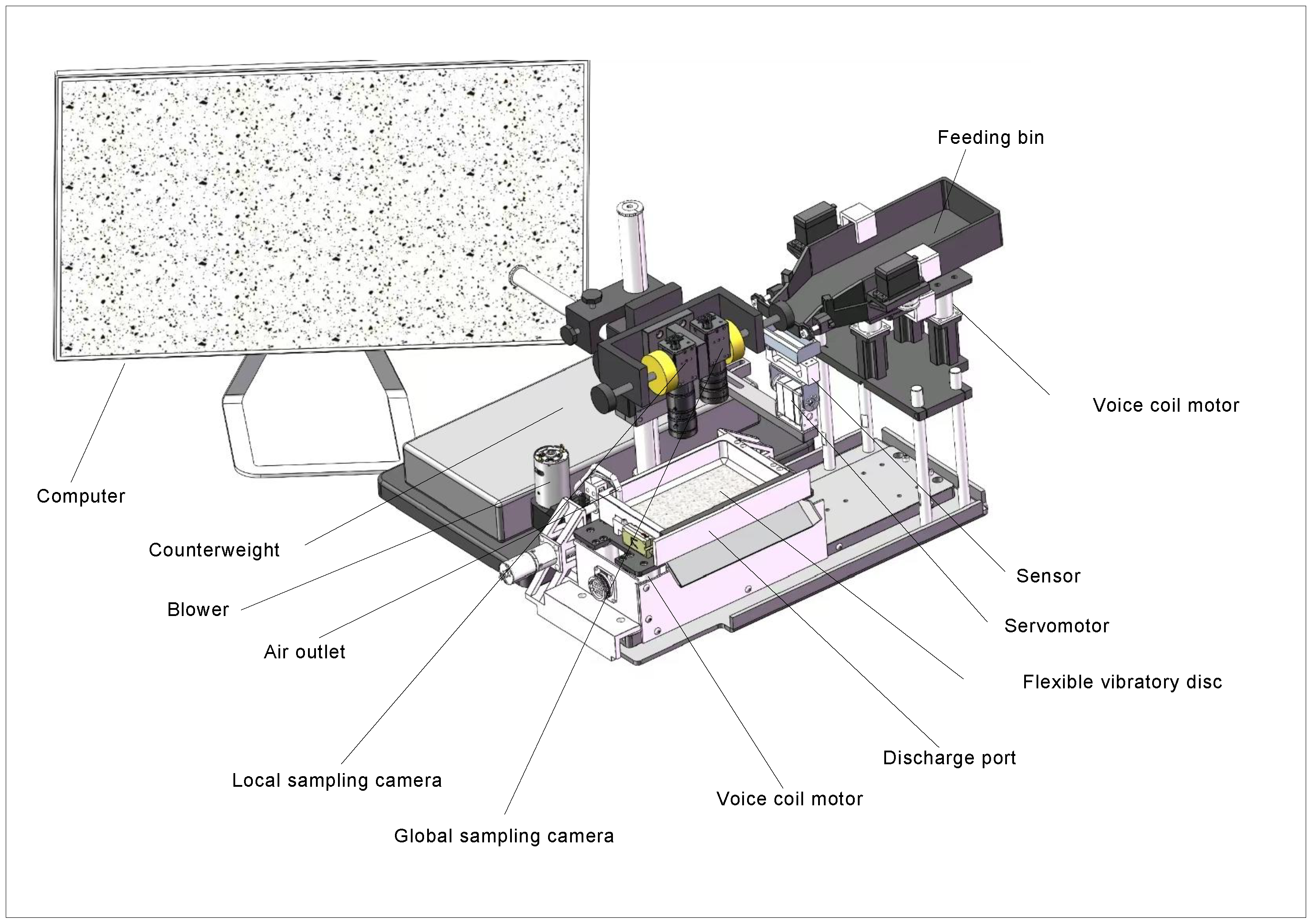
The dual-camera module is also optimised. A wide-angle global camera and high-magnification local camera, synchronised by a PLC, capture complementary views: the global camera records overall distribution, while the local camera resolves micro-scale detail. Compared with frame-by-frame stitching, this configuration achieves full coverage with fewer images and significantly less operating time. Figure 1 shows the overall schematic diagram of the sampling device components.

Under current settings, each sample cycle requires about 2 s for weighing and feeding, 4 s for release, 3 s for vibration dispersion, 1 s for imaging, and 5 s for pneumatic cleaning, totalling roughly 15 s per sample. Detailed camera parameters are listed in

Table 1. Imaging module parameter settings.

Parameter	Global Camera (MV-CS060-10GC)	Local Camera (MV-CS200-10GC)
Focal Length (mm)	12	50
Resolution (pixels)	3072 × 2048	5472 × 3648
Field of View (cm)	10.9 × 7.5	3.8 × 2.6
Frame Rate (fps)	15	8
Pixel Size (µm)	35.2	6.8
Detection Objective	Overall Distribution Statistics	Fine-grained Morphology Analysis

.

Although a single acquisition now completes in 15 s, exhaustively scanning all 334 groups in a 500 g batch would still take over 1.3 h. TISS removes this bottleneck by sampling at fixed intervals (interval): assuming an approximately uniform tray distribution, the system acquires images only once every interval groups, where “interval” is a predefined sampling parameter. Skipping the intervening feed–imaging cycles reduces both image count and runtime. For example, at interval = 10  only 34 groups are captured, and the batch time drops to 8.5 min—a 16-fold speed-up compared to the original 2.13 h.

Under this constraint, combining TISS with single-frame sampling reduced the batch time to 8 min while keeping the total gradation error under 12%, meeting the requirements for rapid on-site grading in industrial settings.

3.2. Image Processing

3.2.1. Block-Wise Adaptive Threshold Segmentation

Complex backgrounds and uneven lighting can complicate the extraction of sand-particle contours from images. Texture artefacts, brightness gradients, and sensor noise are common in our setup, and the edges of particles smaller than 0.15 mm are easily lost in the background. Conventional single-frame global thresholding fails under these conditions because it cannot adjust to local brightness variations or preserve the boundaries of very small particles.

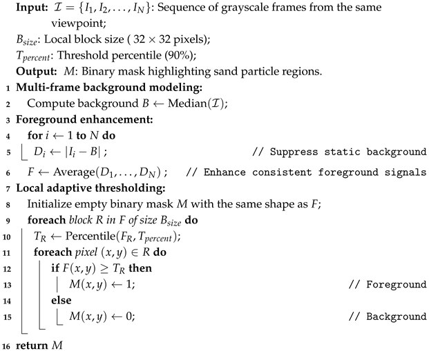
To overcome these limitations, we introduce a two-stage background-suppression scheme that combines multi-frame background modelling with block-wise adaptive thresholding. First, consecutive frames are fused to isolate the stable background component, thereby suppressing fixed-pattern noise and repetitive texture. The resulting averaged image serves as an accurate background estimate. Next, the image is partitioned into local blocks, and each block is thresholded based on its luminance statistics, enabling localised binarisation. In essence, multi-frame fusion yields a clean background, while block-wise adaptation compensates for spatial illumination differences. Together, these steps greatly improve the retention and boundary integrity of fine particles in complex scenes. Pseudocode for the full segmentation procedure is given in Algorithm 1.

Algorithm 1: Multi-frame Adaptive Sand Particle Segmentation

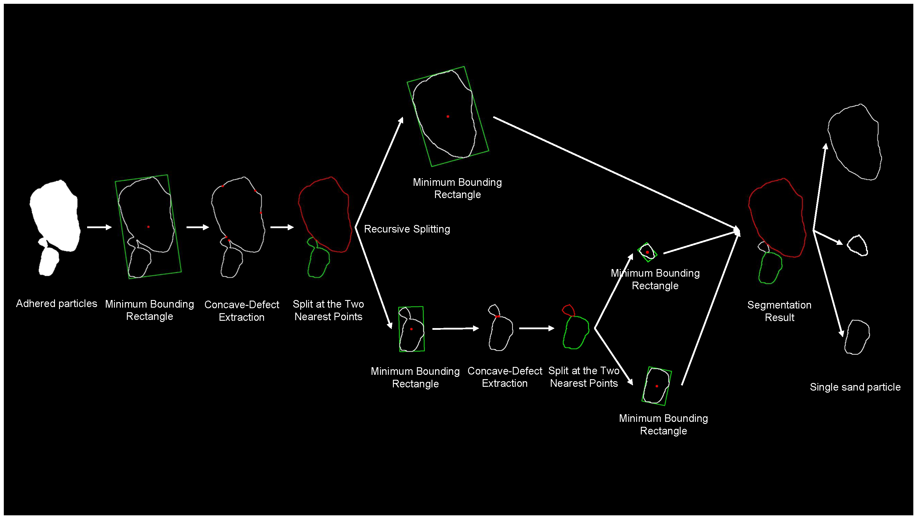
3.2.2. Recursive Concavity-Guided Segmentation (RCGS)

Following background suppression and thresholding, adhered or touching particles must be separated to isolate individual grains. To accomplish this, the RCGS algorithm is employed, utilizing efficient, rule-based techniques to accurately identify and segment adhered particles. The overall process is outlined in Figure 2.

(1)

Adhesion Determination.

Before segmenting a particle cluster, RCGS first assesses whether a given contour corresponds to a single grain or an adhered aggregate. This decision uses a hybrid approach combining geometric descriptors—such as aspect ratio, solidity, and convexity—with an analysis of concave regions along the contour. If the metrics indicate a single particle, the contour remains unchanged; otherwise, segmentation proceeds.

(2)

Iterative Concavity-Based Splitting.

For identified adhered clusters, RCGS iteratively splits the contour along lines connecting pairs of significant concave points. At each iteration, the closest pair of concave points (based on Euclidean distance) is selected, and the particle is bisected accordingly. Each resulting sub-contour is then re-evaluated using the adhesion criteria from step (1).

(3)

Recursion and Termination.

This split-and-check cycle recurses until all contours satisfy the single-particle criteria or can no longer be divided by concavity rules. By combining precise adhesion detection with recursive splitting, RCGS effectively separates complex particle clusters without relying on training data. Compared to fixed-threshold or morphology-based methods, RCGS offers enhanced adaptability and produces physically meaningful segmentation boundaries.

Overall, the RCGS pipeline integrates concave-defect detection, nearest-point splitting, and iterative refinement, enabling reliable decomposition of adhered particles with complex shapes. As shown in Figure 3, the method successfully separates merged contours into individual, geometrically consistent grains.

3.3. Gradation Calculation

3.3.1. Particle Size Classification

To enhance the accuracy and automation of particle size classification in image-based gradation analysis, we propose a statistically robust and computationally efficient interval-division method. Assuming particle sizes approximately follow a normal distribution, this approach combines single-size sample experiments with probabilistic modelling to determine classification boundaries. This data-driven method avoids the subjectivity and misclassification risks inherent in empirical size thresholds.

Specifically, sand samples were first separated by standard sieve analysis into well-defined size intervals. High-resolution images of each single-size sample were then acquired, extracting the Feret diameter of individual, well-formed particles while excluding agglomerates and incomplete edge particles. Each size group’s diameter distribution was found to be unimodal and approximately normal. Adjacent size groups showed minimal overlap; thus, classification boundaries were set at the intersections of their fitted probability density functions, minimising misclassification risk between neighbouring classes.

Practically, for each size interval (e.g., 0.075–0.15 mm and 0.15–0.3 mm), multiple images were collected, and Feret diameter histograms were plotted. The mean ($\mu$) and standard deviation ($\sigma$) of each group defined its normal distribution. Overlaying the probability density curves of adjacent intervals, the intersection points were computed as optimal classification thresholds.

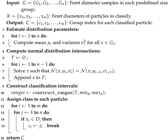
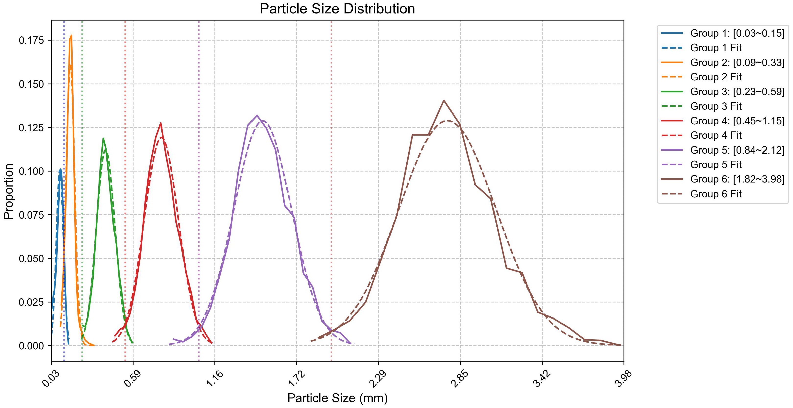
By numerically determining these intersection points for all adjacent pairs, six size thresholds were established to segment the full particle size range. As shown in Figure 4, these thresholds align closely with conventional sieve grading standards and effectively reduce misclassification. The complete classification procedure is detailed in Algorithm 2.

Figure 4 illustrates the empirical data points (solid markers) alongside their fitted normal-distribution curves (dashed lines) for each size interval, with a detailed explanation of the fitting process provided below.

Explanation of Plotting Procedure: First, all detected sand particles were classified into six predefined size intervals based on their short Feret diameter (e.g., 0.075–0.15 mm, 0.15–0.30 mm, …, 2.36–4.75 mm). Within each interval, the range of short Feret diameters was divided into 20 equal-width bins. We then counted the number of particles in each bin and normalized these counts according to the total particle count in the interval to obtain relative frequencies. These frequencies, plotted as solid markers at bin centres, represent the empirical particle size distribution for each interval. Finally, we calculated the sample mean and standard deviation of the short Feret diameters in each interval and fitted a continuous normal (Gaussian) curve using these parameters (depicted as dashed lines). This process was repeated for all six intervals, resulting in the overlaid empirical distributions and fitted curves shown in Figure 4.

Algorithm 2: Feret Diameter-Based Particle Size Classification

Unlike fixed-ratio or empirically set thresholds, this statistically driven method builds classification boundaries solely from actual image data. It eliminates the need for manual tuning or subjective parameters, enhancing adaptability and robustness across different sand batches. This advantage is especially significant for fine aggregates with continuous size distributions and overlapping ranges. By minimizing misclassification risk, the approach provides a reliable foundation for accurate gradation calculation.

3.3.2. Dual-View Fusion and Correction

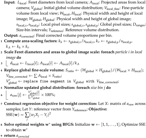
Even after size classification, combining the data from the two different camera views requires careful calibration to avoid bias. We developed a three-stage compensation and correction strategy for dual-view fusion, consisting of scale normalization, view substitution, and error correction.

Scale Normalization: Camera calibration established the physical length per pixel in horizontal and vertical directions for both global and local cameras, producing scaling factors for each view. Since particle orientations vary randomly, simple one-dimensional scaling risks directional bias. To mitigate this, we apply an orientation-independent mapping that statistically aligns the Feret diameters measured by the local camera with the global scale via weighted averaging. For-particle projection areas, a two-dimensional scaling factor, maps local areas to the global scale. Given the global and local cameras’ differing fields of view, the local fine-particle volume is amplified proportionally to the area ratio, ensuring proper scaling of the local camera’s contribution.

Fine-Particle Replacement: Assuming uniform particle dispersion due to vibration-assisted sample spreading, the local camera’s field of view is considered representative for particles smaller than 0.3 mm. Therefore, we replace all <0.3 mm size data in the global image with measurements from the local camera, compensating for the global camera’s limited resolution in this range. After substitution, the combined particle size distribution is normalized so that the total volume fraction sums to 100%, forming the initial fused gradation profile.

Weighted Error Correction: To correct residual systematic deviations between cameras, we introduce a weight vector ($W=(w_1,w_2,\dots )$) applied to the normalized fused gradation vector ($X=(X_1,X_2,\dots )$), aiming to minimize the squared error relative to the ground-truth sieve analysis ($Y=(Y_1,Y_2,\dots )$). The objective function is

$$\mathrm{SSE}\left(W\right)=\sum _j{(w_j{X}_j-Y_j)}^2.$$

We solve this using a quasi-Newton BFGS optimization to find the optimal weights ($W^{*}$), which are then applied to X to yield the final corrected gradation.

With this three-stage fusion strategy—fine-particle replacement, global normalization, and weighted error correction—we fully exploit the complementary strengths of the dual-camera system. The global view ensures comprehensive coverage of particle sizes, while the local view provides high-resolution detail for the fine particle range. The final fused result achieves high accuracy for the fine particles without sacrificing consistency in the overall distribution. In our implementation, this approach significantly reduced the number of images required and shortened the detection duration, yet it still enabled high-precision reconstruction of the full-range particle gradation. It provides an efficient and reliable framework for rapid fine-aggregate gradation analysis in engineering applications. (The detailed pseudocode for the fusion and correction procedure is presented in Algorithm 3).

Algorithm 3: Weighted Correction of Fine-Scale Particle Volume Distribution

4. Results and Analysis

This study focuses on manufactured sand fine aggregates with particle sizes ranging from 0.075 mm to 4.75 mm. A total of ten 500 g sand samples were collected for gradation experiments. Additionally, systematically captured single-size samples were obtained: for the 0.075–0.15 mm and 0.15–0.3 mm intervals, 50 sample groups were collected, each comprising 10 images; for the 0.3–4.75 mm range, 20 sample groups per size interval were collected, each also imaged 10 times.

To comprehensively evaluate the effectiveness and practical applicability of the proposed method, two key metrics were adopted: grading error, which quantifies deviations in overall particle size distribution fitting, and fineness-modulus error, reflecting shifts in the distribution trend. Based on these metrics, three sets of experiments were designed to assess the performance of the image-based detection method under various strategies and parameter settings.

First, sampling efficiency optimization experiments were conducted using 500 g batches of mixed manufactured sand. These experiments evaluated the impact of the TISS technique and a multi-frame burst imaging scheme with varying sampling intervals and frame counts on detection time and grading error, thereby validating the feasibility of reducing image quantity while maintaining sample representativeness.

Second, a dual-camera fusion comparison experiment was carried out, wherein gradation results were calculated from global images, local images, and their fusion. This was intended to investigate the effectiveness of multi-scale collaborative imaging in compensating for fine particles and enhancing overall accuracy.

Finally, segmentation strategy comparison experiments were performed, contrasting four approaches: no segmentation, direct elimination, fixed thresholding, and dynamic judgment. These experiments demonstrated the robustness and accuracy of the proposed recursive segmentation algorithm under complex particle adhesion scenarios.

4.1. Efficiency Optimization Comparison Experiment

To assess the trade-off between efficiency and accuracy achieved by the proposed acquisition optimizations, we conducted a sampling efficiency experiment using 500 g batches of standard manufactured sand. Since the vibration dispersion plate could only accommodate approximately 1.5 g of sand per operation, multiple feeding and imaging cycles were required to cover the entire 500 g sample. In these tests, the dual-camera system was employed to ensure image quality while exploring methods to reduce the total number of images and, thus, improve detection efficiency. In particular, a single-frame sampling approach was adopted, where only the first image captured in each feeding cycle was retained to represent that group. This formed the basis for analysing different sampling intervals.

Using this single-frame-per-group baseline, we further investigated various frame intervals. The interval parameter (interval = 1, 2, …, 20) indicated that one image was retained out of every specified number of consecutive frames in the original sequence. Thus, larger interval values simulated more aggressive data reduction. Although our final optimized strategy retained only one image per group, in this experiment, the retained images were partitioned into multiple equal-sized groups (based on the interval) for comparative analysis.

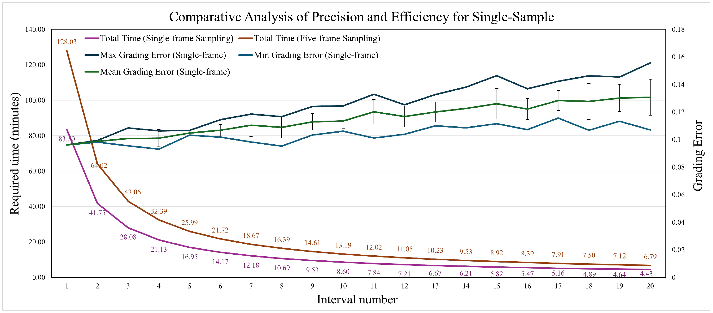
This approach allowed us to assess the internal consistency and stability of grading results at different sampling densities. For each interval, the minimum, maximum, and average gradation errors were calculated to evaluate how image sampling density affected detection accuracy and robustness (see

Table 2. Raw metrics for the single-frame strategy at different sampling intervals.

Interval	Max Error (%)	Min Error (%)	Average Error (%)	Std Dev	Time (min)
1	9.62	9.62	9.62	0	83.50
2	9.94	9.82	9.88	0.0008	41.75
3	10.85	9.56	10.09	0.0068	28.08
4	10.64	9.31	10.11	0.0062	21.13
5	10.67	10.32	10.48	0.0016	16.95
6	11.44	10.18	10.68	0.0043	14.17
7	11.85	9.83	11.04	0.0081	12.18
8	11.67	9.53	10.89	0.0077	10.69
9	12.41	10.34	11.29	0.0059	9.53
10	12.46	10.61	11.35	0.0052	8.60
11	13.29	10.11	12.02	0.0089	7.84
12	12.53	10.39	11.68	0.0076	7.21
13	13.27	10.99	12.01	0.0074	6.67
14	13.82	10.86	12.26	0.0091	6.21
15	14.64	11.16	12.60	0.0111	5.82
16	13.69	10.72	12.22	0.0077	5.47
17	14.24	11.56	12.83	0.0072	5.16
18	14.63	10.68	12.77	0.0131	4.89
19	14.54	11.33	13.02	0.0099	4.64
20	15.58	10.71	13.07	0.0130	4.43

). In the table, “Time” refers to the duration required to analyse the sample, “Error” denotes the mean absolute cumulative gradation error, and “Std Dev” represents the standard deviation of these gradation errors computed from multiple independent sampling runs within the same interval, reflecting measurement consistency and repeatability under that sampling configuration.

Figure 5 illustrates the trade-off between total processing time and grading error as the sampling interval increases. As expected, a larger interval (i.e., fewer images analysed) substantially reduced total detection time but caused a gradual increase in average grading error. Specifically, at an interval of 11, the average grading error remained around 12%, which was acceptable for practical applications, while total processing time was reduced to approximately 7–8 min. This represents more than a 15-fold speed-up compared to using the full image set. However, beyond interval = 11, the error increased sharply (exceeding 18% at interval = 15), compromising reliability. Therefore, an interval of 11 images is recommended as the optimal balance between accuracy and efficiency for our system.

Table 3. Detection time, mass, error, and standard deviation for sampling scheme with 1 image per group.

Interval	Time (min)	Mass (g)	Error (%)	Std Dev
1	83.50	500.00	9.62	0
2	41.75	250.00	9.88	0.0008
3	28.08	166.67	10.09	0.0068
4	21.13	125.00	10.11	0.0062
5	16.95	100.00	10.48	0.0016
6	14.17	83.33	10.68	0.0043
7	12.18	71.43	11.04	0.0081
8	10.69	62.50	10.89	0.0077
9	9.53	55.56	11.29	0.0059
10	8.60	50.00	11.35	0.0052
11	7.84	45.45	12.02	0.0089
12	7.21	41.67	11.68	0.0076
13	6.67	38.46	12.01	0.0074
14	6.21	35.71	12.26	0.0091
15	5.82	33.33	12.60	0.0111
16	5.47	31.25	12.22	0.0077
17	5.16	29.41	12.83	0.0072
18	4.89	27.78	12.77	0.0131
19	4.64	26.32	13.02	0.0099
20	4.43	25.00	13.07	0.0130

,

Table 4. Detection time, mass, error, and standard deviation for sampling scheme with 2 images per group.

Interval	Time (min)	Mass (g)	Error (%)	Std Dev
1	52.88	250.00	9.54	0
2	26.60	125.00	9.93	0.0050
3	18.05	83.33	10.17	0.0033
4	13.62	62.50	10.72	0.0034
5	10.77	50.00	10.84	0.0081
6	9.18	41.67	11.10	0.0073
7	7.92	35.71	11.56	0.0078
8	6.97	31.25	11.76	0.0098
9	6.33	27.78	11.68	0.0106
10	5.70	25.00	12.69	0.0161
11	5.07	22.73	12.30	0.0097
12	4.75	20.83	12.80	0.0118
13	4.43	19.23	13.09	0.0152
14	4.12	17.86	13.52	0.0146
15	3.80	16.67	13.05	0.0121
16	3.48	15.63	13.66	0.0136
17	3.48	14.71	13.74	0.0107
18	3.17	13.89	13.22	0.0161
19	3.17	13.16	13.99	0.0167
20	2.85	12.50	14.93	0.0158

and

Table 5. Detection time, mass, error, and standard deviation for sampling scheme with 3 images per group.

Interval	Time (min)	Mass (g)	Error (%)	Std Dev
1	40.13	166.67	9.83	0
2	20.07	83.33	10.60	0.0026
3	13.62	55.56	10.84	0.0081
4	10.39	41.67	11.21	0.0090
5	8.24	33.33	12.13	0.0075
6	6.81	27.78	12.31	0.0155
7	6.09	23.81	12.43	0.0117
8	5.38	20.83	13.00	0.0115
9	4.66	18.52	12.77	0.0116
10	4.30	16.67	13.26	0.0084
11	3.94	15.15	13.74	0.0195
12	3.58	13.89	13.77	0.0131
13	3.23	12.82	14.17	0.0100
14	3.23	11.90	14.51	0.0216
15	2.87	11.11	14.92	0.0150
16	2.87	10.42	15.62	0.0193
17	2.51	9.80	15.47	0.0141
18	2.51	9.26	15.87	0.0168
19	2.51	8.77	16.27	0.0197
20	2.15	8.33	15.94	0.0165

present the detection time, sampled mass, grading error, and standard deviation for sampling schemes using 1, 2, or 3 images per group across various sampling intervals. Detection time (in minutes) denotes the total duration required to analyse each sampling group. Sampled mass (in grams) represents the approximate weight of sand corresponding to each group, which varies depending on the number of images and the sampling interval. Grading error (percentage) indicates the mean absolute cumulative gradation error, reflecting the deviation from the reference gradation. The standard deviation captures the variability of grading errors computed from multiple independent sampling runs under the same conditions, thereby representing the internal consistency and stability of the results.

Experimental results show that increasing the sampling interval reduced the actual sand mass represented per group, which led to greater random fluctuations and larger grading errors. This effect was especially pronounced when the sampled mass fell below 50 g, thereby compromising the reliability of the results.

Further analysis showed that when each batch maintained a sampled mass of at least 50 g (with interval ≈ 10–11), the randomness in particle distribution was effectively suppressed. Under these conditions, both the grading error and its standard deviation remained well controlled: fluctuations in grading accuracy stayed within ±2%, and the standard deviation of error typically remained below 0.02, indicating stable and representative results. Within these constraints, comparative tests confirmed that—for the same total sampled mass—the single-image-per-group method with TISS required the fewest images and the shortest detection time (approximately 7–8 min per batch). Using a multi-frame burst per group (e.g., capturing 2–3 images per group) yielded only marginal accuracy improvements (reducing error to below 12% and slightly lowering the standard deviation) but incurred significantly higher image counts and longer processing times. Considering the trade-offs among accuracy, stability (in both error and variability), and efficiency, we recommend the single-image-per-group strategy with a moderate interval of 11. This configuration maintained grading error near 12%, kept a low standard deviation of error, and achieved the fastest processing speed, demonstrating strong practical utility for real-time grading in industrial environments.

4.2. Dual-Camera Comparison Experiment

Next, we evaluated the dual-camera fusion strategy’s ability to improve detection accuracy while reducing image acquisition load. Comparative tests were conducted on 500 g standard sand samples, examining three detection schemes across various particle-size intervals. Conventionally, a high-magnification local camera and a wide-angle global camera each capture multiple images (e.g., five consecutive frames) per sample group to average out random particle distribution variations. In contrast, our proposed fusion strategy compensates for missing fine-particle information (<0.3 mm) in the global images by incorporating data from the local images, combined with field-of-view area ratio scaling and volume normalization. Consequently, the fusion approach requires only one image per group to accurately account for the fine fraction and produce a stable overall gradation.

To further validate the robustness of the fusion strategy, we tested one representative sand sample for each of three gradation types: fine-graded, medium-graded, and coarse-graded.

Table 6. Comparison of gradation results for a coarse manufactured sand sample (FM = 3.52) using three computation strategies. (Error denotes mean absolute cumulative gradation error, %).

Particle Size (mm)	0.075–0.15	0.15–0.3	0.3–0.6	0.6–1.18	1.18–2.36	2.36–4.75	>4.75	FM	Error
Reference	4%	2%	16%	22%	22%	28%	0%	3.52	–
Global only	–	–	15.73%	21.21%	27.60%	35.46%	0%	–	11.34%
Local only	3.23%	2.11%	21.36%	23.12%	24.39%	25.78%	0%	3.41	13.20%
Fusion	3.22%	2.34%	18.56%	21.72%	25.17%	28.99%	0%	3.50	7.77%

,

Table 7. Comparison of gradation results for a coarse manufactured sand sample (FM = 2.51) using three computation strategies. (Error denotes mean absolute cumulative gradation error, %).

Particle Size (mm)	0.075–0.15	0.15–0.3	0.3–0.6	0.6–1.18	1.18–2.36	2.36–4.75	>4.75	FM	Error
Reference	13%	9%	27%	26%	15%	10%	0%	2.51	–
Global only	–	–	29.96%	29.97%	23.57%	16.50%	0%	–	16.04%
Local only	14.05%	9.77%	32.83%	21.78%	14.18%	7.39%	0%	2.34	15.29%
Fusion	15.18%	11.94%	25.70%	22.42%	14.95%	9.81%	0%	2.39	10.24%

and

Table 8. Comparison of gradation results for a coarse manufactured sand sample (FM = 2.01) using three computation strategies. (Error denotes mean absolute cumulative gradation error, %).

Particle Size (mm)	0.075–0.15	0.15–0.3	0.3–0.6	0.6–1.18	1.18–2.36	2.36–4.75	>4.75	FM	Error
Reference	20%	10%	29%	31%	10%	0%	0%	2.01	–
Global only	–	–	37.26%	41.73%	17.61%	3.4%	0%	–	13.44%
Local only	17.85%	10.87%	31.44%	28.83%	9.31%	1.69%	0%	2.06	10.00%
Fusion	18.12%	12.51%	29.09%	28.31%	10.12%	1.86%	0%	2.05	9.14%

present the gradation and fineness-modulus errors obtained with the three methods: local only, global only, and fusion. In each case, the local-only method uses only the high-resolution camera data, the global-only method uses only the wide-angle camera data, and the fusion method combines both via our dual-view algorithm.

For the coarse sand sample (FM = 3.52), the average detection error based on five local camera images was 13.20%. The global camera, after excluding particles smaller than 0.3 mm, achieved a reduced error of 11.34%. In comparison, the fusion strategy—which uses only a single local image to compensate for the fine particle range—further decreased the overall error to 7.77%, outperforming both the local-only and global-only methods. This demonstrates that the fusion approach not only reduces the number of images required but also improves the accuracy of gradation estimation.

For the medium sand sample (FM = 2.51), the local-only scheme exhibited an error of 15.29%, while the global-only approach showed an even higher error of 16.04%, reflecting size deviations under moderate fineness conditions. In contrast, the fusion strategy lowered the error to 10.24%, confirming its accuracy advantage, even with a more uniform particle size distribution.

In the fine sand sample (FM = 2.01), errors from the local-only and global-only methods were 10.00% and 13.44%, respectively, highlighting inconsistencies in fine particle measurements when using a single imaging path. The fusion strategy further reduced the error to 9.14%, the lowest among the three methods, validating the importance of high-resolution imaging in compensating for the finest particle fractions.

Overall, comparisons across the three sample types demonstrate that the fusion strategy, while maintaining high acquisition efficiency by relying on just a single local image, achieves significant error reductions—up to 42.9% compared to the local-only method. This highlights its superior adaptability and robustness, confirming its accuracy advantage and practical feasibility as an industrial online detection solution.

Figure 6 illustrates the fineness-modulus error and gradation error across ten sample groups for the three methods. The local camera method (local only) generally exhibited higher errors, with significant fluctuations between groups, indicating insufficient statistical stability. While the global camera method (global only), which excludes fine particles, slightly reduced the average error, it still showed noticeable variation and failed to address the omission of fine particles. In contrast, the fusion strategy achieved the lowest errors in the vast majority of samples, with deviations controlled within ±2%, demonstrating superior consistency and robustness. These results indicate that the fusion approach significantly improves detection accuracy while reducing the number of required images.

Table 9. Gradation error and FM error for three methods (global only, local only, and fusion) by sample.

Sample	Global Only		Local Only		Fusion
	Error	FM Error	Error	FM Error	Error	FM Error
1	11.34%	0.1045	13.20%	$-0.1133$	7.77%	$-0.0175$
2	7.92%	0.7270	10.18%	0.1321	7.65%	0.0629
3	13.86%	0.1458	12.06%	0.0263	5.76%	$-0.0637$
4	15.98%	0.2040	19.50%	$-0.0620$	10.15%	0.1574
5	18.67%	0.2220	10.38%	0.2142	6.50%	0.1056
6	13.33%	0.1047	26.22%	$-0.1121$	15.37%	$-0.0127$
7	16.04%	0.1635	15.29%	$-0.1655$	10.24%	$-0.1156$
8	19.65%	0.2015	9.63%	0.1009	10.71%	0.0977
9	22.65%	0.2641	8.57%	$-0.0411$	12.87%	0.0713
10	13.44%	0.1429	10.00%	0.0495	9.14%	0.0435
Std Dev	0.0428	0.0601	0.0553	0.1224	0.0294	0.0451

presents detailed gradation error and fineness-modulus (FM) error values for each sample group, along with the overall standard deviations computed from the ten samples per group. The gradation error reflects the cumulative deviation in particle size distribution, while the FM error measures deviations in the fineness modulus. The standard deviations indicate the variability of errors across the ten samples, highlighting the fusion strategy’s advantage in achieving both lower average errors and improved consistency compared to the other methods.

4.3. Segmentation Algorithm Comparison Experiment

The performance of image-based particle segmentation algorithms directly impacts the accuracy of gradation analysis. To evaluate the effectiveness of the proposed dynamic thresholding combined with the RCGS segmentation strategy, four comparison schemes were designed to analyse differences in particle identification and gradation outcomes:

Selectively removing large contours identified as aggregates while retaining small clusters containing only a few particles;

Retaining strictly single-particle contours, deleting all regions classified as aggregates.

Applying a fixed global shape-factor threshold, accepting contours above the threshold as single particles and forcibly splitting those below it via convex-hull or defect analysis.

Employing size-adaptive thresholds that tighten for large particles and relax for small ones, thereby mitigating projection- or noise-induced misclassification and reducing over-segmentation.

In

Table 10. Comparison of four image processing strategies for gradation computation on coarse manufactured sand (Mx = 3.52). (Error denotes mean absolute cumulative gradation error, %).

Method	0.075–0.15	0.15–0.3	0.3–0.6	0.6–1.18	1.18–2.36	2.36–4.75	>4.75	FM	Error
Reference	4%	2%	16%	22%	28%	28%	0%	3.52	–
$m_1$	4.09%	4.56%	21.75%	24.79%	21.14%	23.67%	0%	3.25	–
${\Delta }_1$	−0.09%	−2.56%	−5.75%	−2.79%	6.86%	4.33%	0%	–	22.38%
$m_2$	3.90%	3.37%	19.18%	22.09%	23.43%	28.03%	0%	3.42	–
${\Delta }_2$	0.10%	−1.37%	−3.18%	−0.09%	4.57%	−0.03%	0%	–	9.34%
$m_3$	3.83%	3.41%	19.02%	21.82%	23.57%	28.35%	0%	3.43	–
${\Delta }_3$	0.17%	−1.41%	−3.02%	0.18%	4.43%	−0.35%	0%	–	9.56%
RCGS	3.22%	2.34%	18.56%	21.72%	25.17%	28.99%	0%	3.50	–
${\Delta }_4$	0.78%	−0.34%	−2.56%	0.28%	2.83%	−0.99%	0%	–	7.77%

, the gradation errors corresponding to the four segmentation strategies are denoted as $m_1$, $m_2$, $m_3$, and RCGS. Specifically, $m_1$ corresponds to selective removal of only large aggregate contours while retaining small clusters; $m_2$ refers to strict single-particle retention, deleting every contour identified as an aggregate; $m_3$ applies a fixed global shape-factor threshold and forcibly splits contours falling below it via convex analysis; and RCGS uses a size-adaptive shape-factor threshold that tightens for large particles and relaxes for small ones, thereby mitigating projection- or noise-induced misclassification.

Furthermore, ${\Delta }_i$ ($i=1,\dots ,4$) denotes the retained percentage error in each particle-size interval under the i-th segmentation strategy; a “+” sign indicates underestimation (calculated < actual), while a “−” sign indicates overestimation (calculated > actual). In particular, ${\Delta }_1$ corresponds to strategy $m_1$, ${\Delta }_2$ to $m_2$, ${\Delta }_3$ to $m_3$, and ${\Delta }_4$ to RCGS.

Table 11. Gradation error and FM error for four methods (m1–m3 and RCGS) by sample.

Sample	m1		m2		m3		RCGS
	Error	FM Error	Error	FM Error	Error	FM Error	Error	FM Error
1	22.38%	$-0.2667$	9.34%	$-0.1012$	9.56%	$-0.0907$	7.77%	$-0.0175$
2	21.01%	$-0.1732$	9.55%	$-0.0462$	9.43%	$-0.0390$	7.65%	0.0629
3	13.73%	$-0.1700$	10.83%	$-0.1758$	10.16%	$-0.1608$	5.76%	$-0.0637$
4	19.53%	$-0.1691$	9.52%	0.0445	9.85%	0.0632	10.15%	0.1574
5	15.15%	$-0.1682$	8.86%	$-0.1061$	9.28%	0.1134	6.50%	0.1056
6	33.28%	$-0.3502$	16.96%	$-0.2007$	16.71%	$-0.1927$	15.37%	$-0.0127$
7	26.68%	$-0.2926$	20.16%	$-0.2632$	20.20%	$-0.2575$	10.24%	$-0.1156$
8	22.45%	$-0.2340$	23.64%	$-0.2032$	23.21%	$-0.1981$	10.71%	0.0977
9	25.03%	$-0.1300$	21.03%	$-0.0592$	22.23%	$-0.0498$	12.87%	0.0713
10	27.51%	$-0.0208$	25.05%	$-0.0586$	25.62%	$-0.0563$	9.14%	0.0435
Std	0.0584	0.0927	0.0655	0.0788	0.0668	0.0757	0.0294	0.0451

presents the gradation error and fineness-modulus (FM) error for four segmentation methods (m1–m3 and RCGS) across ten samples. The Error columns indicate the mean absolute cumulative gradation error (expressed as a percentage), while the FM Error columns show deviations in fineness modulus. The final row lists the standard deviations calculated from the ten samples per method, reflecting the variability and stability of each approach.

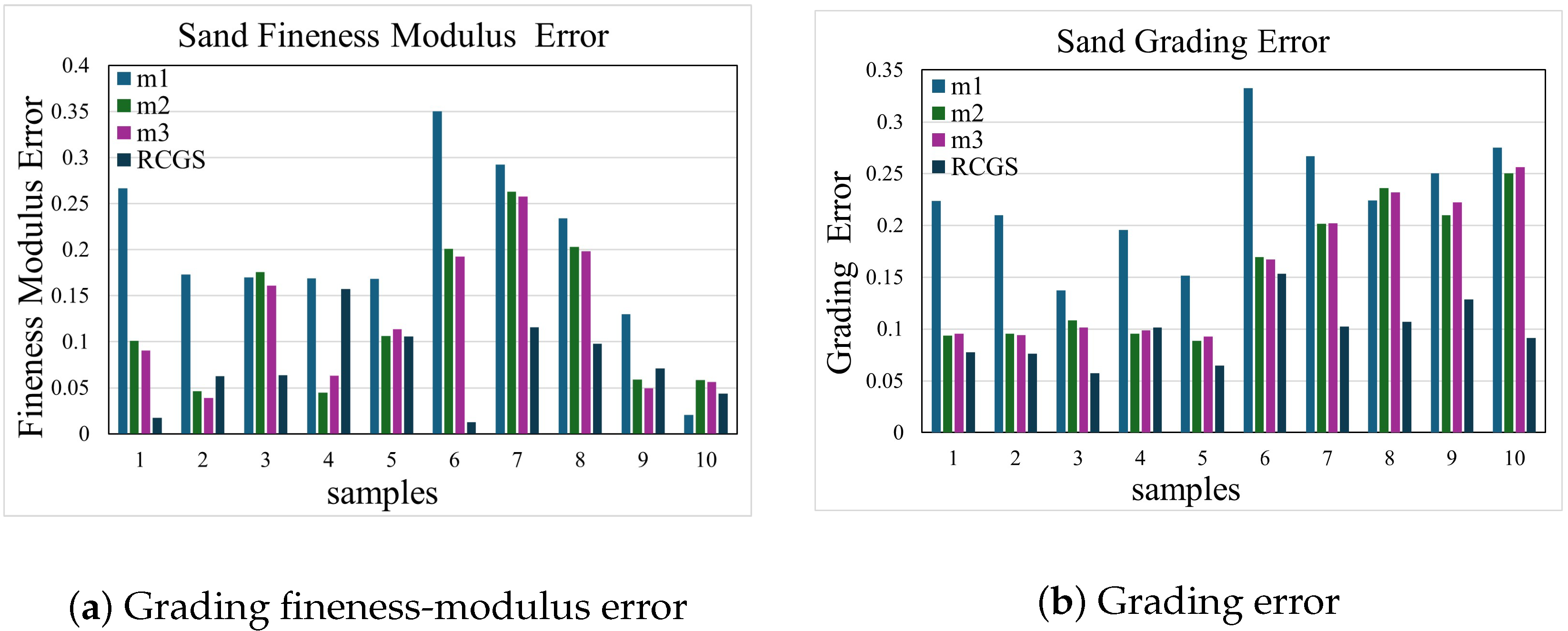
Figure 7 and Table 11, together, demonstrate that RCGS outperforms the other three methods in both gradation and fineness-modulus accuracy. In Figure 7a, the FM error bars for RCGS cluster tightly around zero, indicating minimal deviation, whereas m1, m2, and m3 exhibit larger fluctuations. Table 11 quantitatively confirms this pattern, with RCGS showing a substantially lower maximum absolute FM error compared to m1, m2, and m3. A similar trend is observed in Figure 7b for gradation error, where RCGS consistently achieves the smallest bias.

In practical terms, method m1’s fixed-threshold approach tends to over-delete fine particles, while m2’s complete-deletion scheme underestimates fine-particle content. Method m3 mitigates these extremes by applying a uniform shape-factor threshold but still misclassifies some aggregates. In contrast, RCGS employs a size-adaptive threshold that effectively preserves small particles and accurately separates larger aggregates. This balanced strategy leads to the lowest and most consistent errors without requiring training data, making RCGS the preferred segmentation method.

5. Conclusions

This study addressed the efficiency bottlenecks of manufactured sand gradation detection in industrial applications and proposed an image-based gradation analysis strategy focused on optimizing detection timeliness. Systematic innovations and experimental validations were conducted across three key components: sampling strategy, data fusion, and particle segmentation.

First, a TISS-based image acquisition scheme was introduced. Under a fixed total sample mass of 500 g, the original approach requiring 334 groups of continuous imaging was optimized into an interval-based sampling scheme with a tunable parameter. Experimental results showed that when the interval was set to 11 (sampling approximately 45 g of sand), the grading error remained within ±2%, while imaging time was reduced by 80% to under 8 min. This strategy effectively balanced image quantity and detection stability, providing a tunable trade-off between accuracy and speed for online detection systems.

Second, a dual-camera collaborative fusion strategy was developed to integrate global and local perspectives: the global camera captured the overall particle size range, while the local camera focused on high-precision acquisition of particles smaller than 0.3 mm. Through field-of-view area mapping, scale alignment, volume normalization, and weighted correction, the local fine-particle volume compensated for missing fractions in the global images. Comparative experiments on three representative samples demonstrated that the fusion strategy reduced the average error of single-camera methods from up to 15.29% to 9.52%, significantly narrowing error fluctuations across sand types and confirming its robust adaptability.

Finally, at the image processing level, an adaptive recognition and recursive segmentation algorithm was proposed to separate bonded particles based on equivalent Feret diameter. By combining dual-threshold screening using shape factor and solidity with convex-hull indentation analysis and constraint-driven recursive cuts, the method efficiently separated complex aggregates. Compared to fixed-threshold methods, this approach improved both the identification rate and segmentation integrity of bonded particles without relying on training data, providing high-quality contour data for gradation statistics.

In summary, the proposed multi-level optimization strategy significantly improved detection time, error control, and system adaptability. Without compromising accuracy or stability, it elevated the efficiency of image-based manufactured sand gradation detection to a new industrial standard. This study primarily focused on manufactured sands conforming to Chinese national standards for construction sand, characterized by particle sizes ranging from 0.075 mm to 4.75 mm and low clay impurity levels. The applicability of the proposed method to other sand types, such as recycled concrete aggregates or sands with higher clay and cohesive contents, requires further investigation. Future work will aim to extend and validate the method for these materials to enhance its practical versatility. This study provides significant practical value for rapid deployment and engineering applications, laying a solid foundation for future advancements in intelligent aggregate detection systems.