Article

Machine Learning-Based Methods for the Seismic Damage Classification of RC Buildings †

Department of Construction, Environment and Engineering, Technological and Higher Education Institute of Hong Kong, Hong Kong, China
This paper is an extended version of the paper published in 2023 World Congress on Advances in Structural Engineering and Mechanics (ASEM23), Seoul National University, Seoul, Republic of Korea, 16–18 August 2023.
Buildings 2025, 15(14), 2395; https://doi.org/10.3390/buildings15142395
Submission received: 21 May 2025 / Revised: 26 June 2025 / Accepted: 5 July 2025 / Published: 8 July 2025
(This article belongs to the Section Building Structures)

Abstract

This paper aims to investigate the feasibility of machine learning methods for the vulnerability assessment of buildings and structures. Traditionally, the seismic performance of buildings and structures is determined through a non-linear time–history analysis, which is an accurate but time-consuming process. As an alternative, structural responses of buildings under earthquakes can be obtained using well-trained machine learning models. In the current study, machine learning models for the damage classification of RC buildings are developed using the datasets generated from numerous incremental dynamic analyses. A variety of earthquake and structural parameters are considered as input parameters, while damage levels based on the maximum inter-story drift ratio are selected as the output. The performance and effectiveness of several machine learning algorithms, including ensemble methods and artificial neural networks, are investigated. The importance of different input parameters is studied. The results reveal that well-prepared machine learning models are also capable of predicting damage levels with an adequate level of accuracy and minimal computational effort. In this study, the XGBoost method generally outperforms the other algorithms, with the highest accuracy and generalizability. Simplified prediction models are also developed for preliminary estimation using the selected input parameters for practical usage.

1. Introduction

Assessing the seismic vulnerability of buildings and structures is an important topic in structural engineering. Poorly designed buildings and structures may collapse during strong earthquakes, causing significant loss of life and property. Structural damage under frequent earthquakes may lead to vast economic impacts on society. Vulnerability assessments for buildings are an important tool for assisting the future planning of retrofitting after earthquakes. Identifying high-risk buildings in a city may help to prepare urgent plans for escape when earthquakes occur. This is crucial for cities with buildings and structures not designed to withstand earthquakes. Therefore, many different studies on seismic vulnerability assessment have been conducted in the literature [1,2,3].
Accurately assessing the performance of buildings and structures under earthquakes is highly important in performance-based seismic design and vulnerability assessment. Owing to the random nature of earthquakes and the uncertainty of building properties, advanced techniques are usually involved in such tasks. Two types of methods, namely non-linear static pushover analysis and non-linear time–history analysis (NLTHA), are commonly adopted in most international codes of practice, such as EC8 [4], FEMA356 [5], and ASCE41 [6]. The former method analyzes structure under monotonic loads with a given load pattern to obtain the force–displacement curve (pushover curve) of the structure and to determine the possible failure mechanisms. This method is computationally efficient and highly simplifies the dynamic phenomenon of buildings under earthquakes [7]. Different modified pushover analyses, such as modal pushover analysis [8] and the extended N2 method [9], have been developed in the literature to enhance its performance.
On the other hand, NLTHA determines the structural performance of buildings through the direct numerical integration of the equations of motion under earthquakes. In EC8, the mean values of structural responses under at least seven ground motion histories are considered in the design of buildings, taking into account the uncertainty and randomness of earthquakes. To assess the vulnerability of buildings and structures, seismic fragility analysis is normally adopted to predict the probability of structural damage under different levels of earthquakes. In this case, fragility curves can be generated using either historical records or numerical simulation via incremental dynamic analysis (IDA) [10]. The latter method is based on numerous NLTHAs with a gradual increase in the intensity of the earthquake histories [11]. The IDA curves are then constructed based on the results using the selected intensity measure (IM) and engineering demand parameter (EDP). From the IDA curves, the statistical parameters for constructing the fragility curve can be obtained.
Many studies have adopted NLTHAs to assess the detailed performance of buildings under earthquakes. Nazari and Saatcioglu [1] assessed the vulnerability of concrete shear wall buildings using fragility curves obtained using incremental dynamic analysis. Cardone et al. [12] constructed fragility curves for older residential RC buildings in Italy via a hybrid approach, combining loss assessment data with non-linear dynamic analysis. Pandikkadavath et al. [13] studied the robustness of steel moment-resisting frames by evaluating the fragility curves, robustness parameter, and correction for response reduction factors using the IDA and considering material variability. The results are useful for designing buildings that can withstand disproportionate collapse. Pen et al. [14] utilized NLTHA and IDA to assess the performance of a new separable system for tall buildings, which is formed by separating the gravity- and lateral load-resisting systems. Several story drift ratio limits for the new separate systems were proposed and verified in the study. In general, NLTHA is the most precise method, but the computational effort is generally high, and therefore, it is difficult to widely apply this method in daily design projects in which the design requirements may change from time to time. In general, NLTHA requires users to have a deep understanding of highly specialized topics, such as finite element modeling, the non-linear behavior of material, earthquake selections, etc. This method is computationally demanding and time-consuming. If a rapid vulnerability assessment of buildings or regional large-scale assessments are required, NLTHA may not be appropriate.
Recently, the use of machine learning (ML) has become more popular in different engineering disciplines, such as construction management, building control, design and automation, transportation, and sustainability. Pizarro et al. [15] explored the use of convolutional neural networks to generate floor plans based on two independent plan predictions. The results revealed that the ML model can successfully generate wall layouts. Some studies explored the use of ML methods to predict energy usage in buildings [16,17]. Some studies have reviewed the applications of ML technologies in civil, structural, and earthquake engineering [18,19,20,21,22]. ML can be classified into supervised learning, unsupervised learning, and reinforcement learning [23]. The basic idea of the former is to develop ML models for prediction purposes using vast amounts of well-selected labeled datasets. The models can be used for regression and classification. The former is used to predict continuous outputs, while the latter is used to predict discrete outputs.
Supervised learning has been widely applied in the literature. Table 1 summarizes some research studies from the past decade for regression and classification purposes. For regression purposes, ML models were generally used to predict structural responses such as the inter-story drift ratio or parameters of the fragility curve. A variety of structural and seismic parameters were used to develop prediction models based on different ML algorithms. Giovanis et al. [24] proposed the use of neural network-based models to predict the inter-story drift ratio of buildings under earthquakes. Six parameters that were used to describe the backbone curve of plastic hinges were taken as input parameters. The model worked with Monte Carlo simulation to generate IDA curves for determining the fragility curves. The study showed that the neural network-based model was stable and accurate. Morfidis et al. [25] adopted an artificial neural network (ANN) to predict the inter-story drift ratio and damage class of RC buildings, where the damage class was correlated to the maximum inter-story drift ratio. They used 4 structural and 14 ground motion parameters to train the ANN models and investigated different ANN configurations. The outcomes indicated that ANNs could be a reliable method to assess the damage class of RC buildings. Dabiri et al. [26] proposed an ML-based model to predict fragility curve parameters. Several ML models were used, including decision tree (DT), random forest (RF), K-nearest neighbor (KNN), and ANNs. The study adopted seven structural parameters (e.g., construction material, plan area, building height and lateral load-resisting system, building location, damage state, and period) and one soil parameter to train the ML models. It was revealed that DT was the best model in the study. Demertzis et al. [27] investigated the use of ML methods to determine the maximum inter-story drift ratio of buildings. Systematic procedures were proposed for data collection, model training, and validation. A total of 15 ML algorithms, such as DT, gradient boosting, RF, and light gradient boosting machine (LightGBM), were evaluated. The study considered 4 structural parameters (e.g., height, ratios of base shear received by walls in both directions, and eccentricity) and 14 seismic parameters (e.g., peak ground acceleration and Arias intensity). The results indicated that LightGBM had the highest generalizability and convergence stability among all models under consideration. Shahnazaryan et al. [28] used ML methods for the prediction of collapse and non-collapse responses of buildings. The authors prepared the training dataset using OpenSeesPy based on non-linear SDOF systems. During the training of ML models, six structural parameters, which were used to describe the backbone curves of the SDOF systems, were adopted. The dynamic strength ratio, which was dependent on the average spectral accelerations, was selected as output. The study showed that eXtreme gradient boosting (XGBoost) and DT performed the best among all models. A Python-based library was developed based on XGBoost. Demir et al. [29] used tree-based ML methods for predicting the maximum drift ratio for eight-story regular and irregular RC frames. A total of 21 input parameters, including 20 different intensity measures and spectral acceleration in fundamental periods, were adopted in ML training. It was found that RF performed the best among all the methods under consideration. Işık et al. [30] combined the use of ANNs and particle swarm optimization to develop a neural network-based model to estimate the target displacements of reinforced concrete buildings under different limit states. Input parameters, such as PGA and floor number, were used to set up the model. The hybrid models showed excellent performance in predicting the target displacement of buildings. Payán-Serrano et al. [31] developed prediction models using ANNs to estimate the mean, median, and standard deviation of the maximum inter-story drift for RC buildings with and without buckling restrained braces. Two input parameters, namely the spectral acceleration and intensity measure, were used. In addition, an ANN model was adopted to predict the ductility and hysteretic energy of single-degree-of-freedom systems based on the seismic coefficient, fundamental period of the building, and intensity measure. Neural network configurations, such as the number of hidden layers and the number of units per layer, were investigated.
On the other hand, damage level classification or collapse state prediction were normally considered in most classification studies. Hwang et al. [32] investigated the use of an ML-based methodology for predicting maximum inter-story drift and classifying the collapse state of buildings. A total of 15 structural modeling-related parameters (e.g., plastic rotations and post-yield strength ratio) and 1 parameter for intensity measure were used. The results showed that models using boosting algorithms, particularly XGBoost, performed well in both regression and classification. Bhatta et al. [33] investigated the use of KNN, RF, DT, support vector machine (SVM), and ANNs to predict damage induced by earthquakes. A total of 10 structural parameters (e.g., number of stories, height of building, and fundamental periods) and 7 earthquake parameters (e.g., peak ground acceleration and spectral accelerations) were used. The results revealed that ML models, particularly RF, were capable of rapidly predicting seismic damage in reinforced concrete buildings. Mahmoudi et al. [34] investigated the use of ML models to identify the damage extent of concrete shear wall structures, where the damage level was associated with plastic hinge rotation. Several ML algorithms, such as SVM and KNN, were selected. In addition, a parametric study was conducted to identify important features for damage classification. It was found that drift, correlation, and modified cumulative absolute velocity were the most important indicators. In the study, KNN performed the best among the several ML algorithms under consideration. The accuracy of damage identification was higher than 90% in most cases. Zhang et al. [35] compared RF, XGBoost, and active ML algorithms for seismic damage classification. In total, 8 structural parameters (no. of stories, story height, no. of bays in both directions, length of bay on both directions, constructed period, and seismic design intensity) and 14 ground motion parameters (peak ground acceleration, effective peak acceleration, peak ground velocity, spectrum intensity, and spectral acceleration) were selected as input parameters. It was found that the accuracy of active machine learning models is higher compared to that of the others. Kostinakis et al. [36] studied the performance of 18 widely used ML algorithms for classifying the damage class of buildings under earthquakes. The damage class was defined based on the maximum inter-story drift ratio. A total of 4 structural parameters (height, ratios of the base shear received by walls in two directions, and eccentricity) and 14 seismic parameters (e.g., peak ground acceleration, Arias intensity, and cumulative absolute velocity) were utilized. An auto hyper-parameter tuning method was proposed. It was found that SVM with the Gaussian kernel algorithm is the most accurate algorithm. Wei et al. [37] adopted a convolutional neural network (CNN) and stacking ensemble method to identify the damage class for mega sub-controlled structure systems. The CNN was used to extract important features from response signals, and the stacking method was then used to classify the results based on different damage levels.
The seismic performance of buildings constructed with different materials is also an important topic. Imam et al. [38] developed prediction models to estimate the maximum inter-story drift ratio of steel structures. In the study, random forest, XGBoost, and ANN were adopted and their performance was compared. Five seismic parameters (e.g., peak ground accelerations, magnitude, and duration) and five structural parameters (e.g., numbers of stories, numbers of bays, and bay length) were selected for training prediction models. The results showed that XGBoost outperformed the others. Asgarkhani et al. [39] adopted a machine learning approach to develop models to predict inter-story, residual inter-story drift, seismic performance curves, and fragility curves for steel buckling-restrained brace frames. Eight ML algorithms were used and compared. The results indicated that stack ML-based models were the most suitable methods and achieved high accuracy. Kazemi et al. [40] explored the use of machine learning to classify the seismic performance of steel diagrid structures with different geometries. The study found that classification models with suitable algorithms, such as decision tree, K-nearest neighbor, and ensemble method, could accurately predict the structural behavior of diagrid structures, providing useful insights for system-level design.
In addition to steel structures, the performance of structural members reinforced using fiber-reinforced polymer (FRP) is also a topic of interest nowadays. To et al. [41] developed ML-based fast-running models to predict the inter-story drift ratio and seismic energy-based damage demand of aramid FRP retrofitted RC columns. Three models, namely the recurrent neural network, adaptive neuro fuzzy inference model, and deep recurrent neural network model, were used. The last model was adopted due to its excellent performance. The influences of input parameters were investigated using the developed model. Babiker et al. [42] investigated the use of machine learning to refine the design formulas for punching shear strength calculation of glass fiber-reinforced polymer (GFRP) flat slab-column connections. A machine learning prediction model was developed using deep neural networks. The feature significance was investigated based on the developed model through connection weight analysis. These important features were used to develop design formulas. Wu et al. [43] studied the seismic performance of GFRP-RC columns retrofitted by precast ultra-high performance concrete plates. The results revealed that such retrofitting can increase the peak load and ductility of members.
Some studies investigated the seismic performance of timber structures. Junda et al. [44] applied ML methods to estimate peak inter-story and roof drifts of cross-laminated timber walled structures. ML algorithms, such as random forest, sequential forward floating selection, and least absolute shrinkage and selection operator, were used. Based on the models, six important input features were finally selected to develop refined ML models to predict seismic response of timber structures. The influences of selected features were studied using SHAP values. Zong et al. [45] investigated the seismic performance and dynamic properties of timber–concrete hybrid structures via response spectrum and elastic time–history analyses. Important responses, such as shear force to weight ratio and inter-story drift ratio, were reported. In addition, in situ tests were conducted to measure the dynamic characteristics of cross-laminated timber floors, such as vertical natural frequency and human-induced vibrations.
In short, the effectiveness of different ML algorithms has been investigated in the literature, but the results are quite diverse. Therefore, further research is required to explore the choice of ML algorithms for prediction tasks. Moreover, selecting suitable input parameters for the training of ML algorithms is another major challenge to be explored. More studies are needed to evaluate the importance of different input parameters for ML model development.
Table 1. Regression and classification studies in the literature.
AuthorsType Best ML AlgorithmInput Parameters
Giovanis et al. [24]Regression Artificial Neural NetworkSix parameters of backbone curves
Morfidis and Kostinakis [25]Regression and classificationArtificial Neural Network4 structural and 14 ground motion parameters
Hwang et al. [32]Regression and classificationXGBoost15 structural modeling-related parameters (e.g., plastic rotations, post-yield strength ratio, energy dissipation capacity)
1 parameter for intensity measure (Sa(T1))
Dabiri et al. [26]RegressionDecision Tree 7 structural parameters (construction materials, plan area, height, lateral resisting system, location, damage state, and period)
1 soil parameter
Bhatta and Dang [33]ClassificationRandom Forest10 structural parameters (no. of stories, height, period, age of buildings, etc.)
7 earthquake parameters (PGA, PGV, PGD, seismic intensity, spectral acceleration, etc.)
Demertzis et al. [27]Regression LightGBM4 structural parameters (height, ratio of the base shear received by walls in two directions, and eccentricity)
14 seismic parameters
Mahmoudi et al. [34]ClassificationK-Nearest NeighborArias intensity, cumulative absolute velocity, modified cumulative absolute velocity, spectral acceleration, energy ratio, drift, and correlation
Kostinakis et al. [36]ClassificationSVM–Gaussian kernel4 structural parameters (height, ratio of the base shear received by walls in two directions, and eccentricity)
14 seismic parameters
Zhang et al. [35]ClassificationActive Machine Learning8 structural parameters (e.g., no. of stories, story height, no. of bays in both directions, length of bay on both directions, constructed period, seismic design intensity)
14 ground motion parameters (e.g., peak ground acceleration, effective peak acceleration, peak ground velocity, spectrum intensity, and spectral acceleration)
Shahnazaryan and Reilly [28]RegressionXGBoost
Decision Trees
6 structural parameters for describing backbone curves of SDOF systems
Demir et al. [29]Regression Random Forest20 ground motion parameters
1 spectral acceleration
Işık et al. [30]Regression Artificial Neural NetworkFloor number
PGA
Payán-Serrano et al. [31]RegressionArtificial Neural NetworkFor RC buildings: spectral acceleration and intensity measure
For SDOF buildings: fundamental period, seismic coefficient, and intensity measure
Wei et al. [37]Classification CNN + Stacking MethodStructural acceleration response signals

Research Scope

In this study, various ML methods are explored for predicting the damage class of RC buildings under earthquakes. Different ML algorithms, including basic ML algorithms, ensemble methods, and artificial neural networks, are investigated to study their performance and effectiveness in the damage classification of buildings. The current study also explores performance enhancement by combining ensemble methods and neural networks together. Different input parameters for representing the characteristics of ground motions and structures are considered in ML model development to assess their contributions to the prediction. Suitable ML algorithms and parameters are selected for developing more efficient models for future applications. The research significance is summarized as follows:
  • Datasets for RC buildings without seismic design considerations are created for ML model development. Accurate ML models are developed for rapidly assessing the damage class of buildings during earthquakes. These are valuable for locations with similar design considerations.
  • A comprehensive investigation is conducted to study the effectiveness of different ML algorithms, such as basic models, ensemble methods, and ANN models, for classifying the damage class of buildings. Efficient methods are identified.
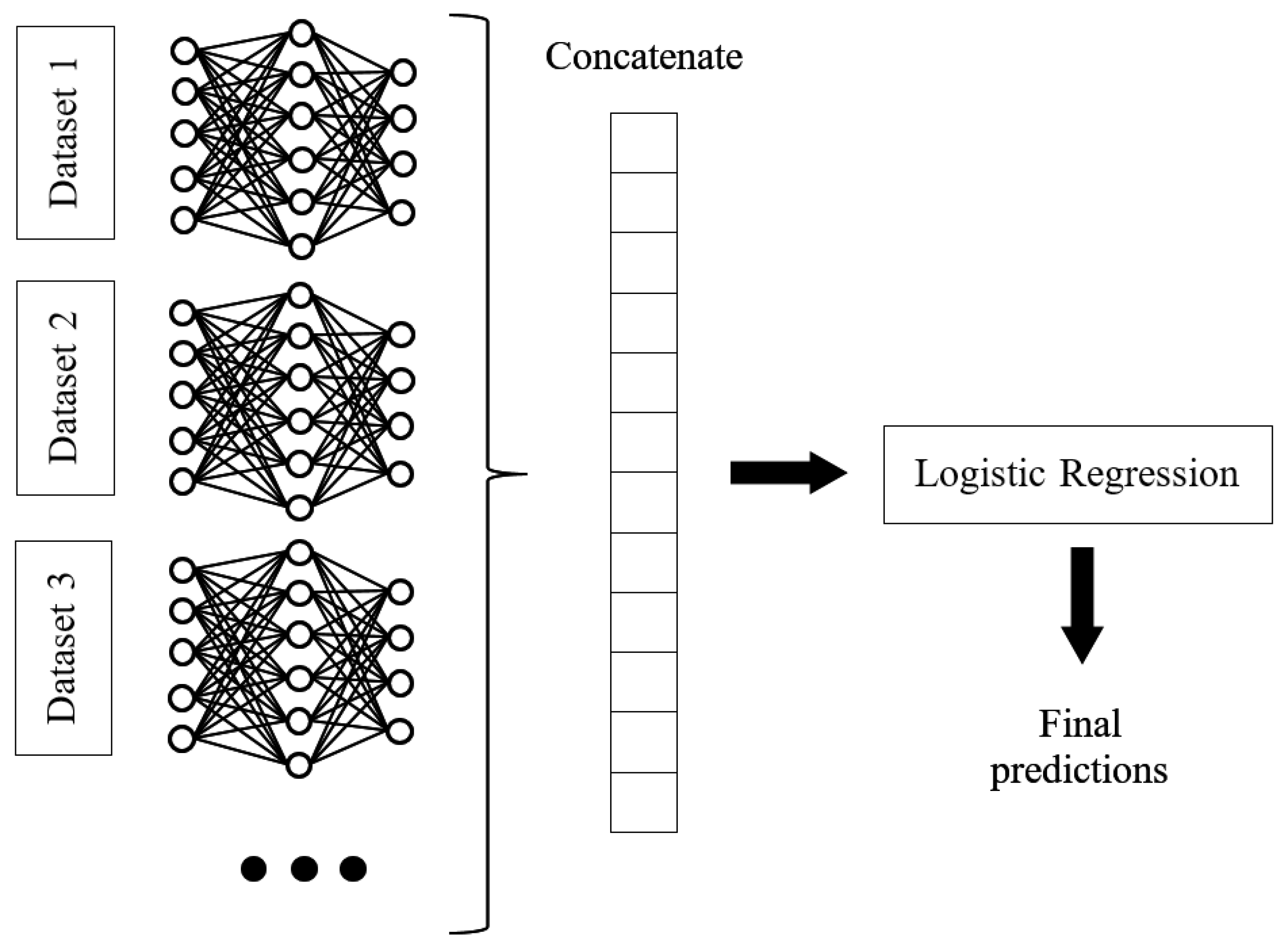
  • Neural network models combined with ensemble methods (stacking and boosting) are used to improve the performance of ANN models to handle tabular data.
  • The importance of input features is examined to identify significant earthquake and structural parameters for refining ML models.
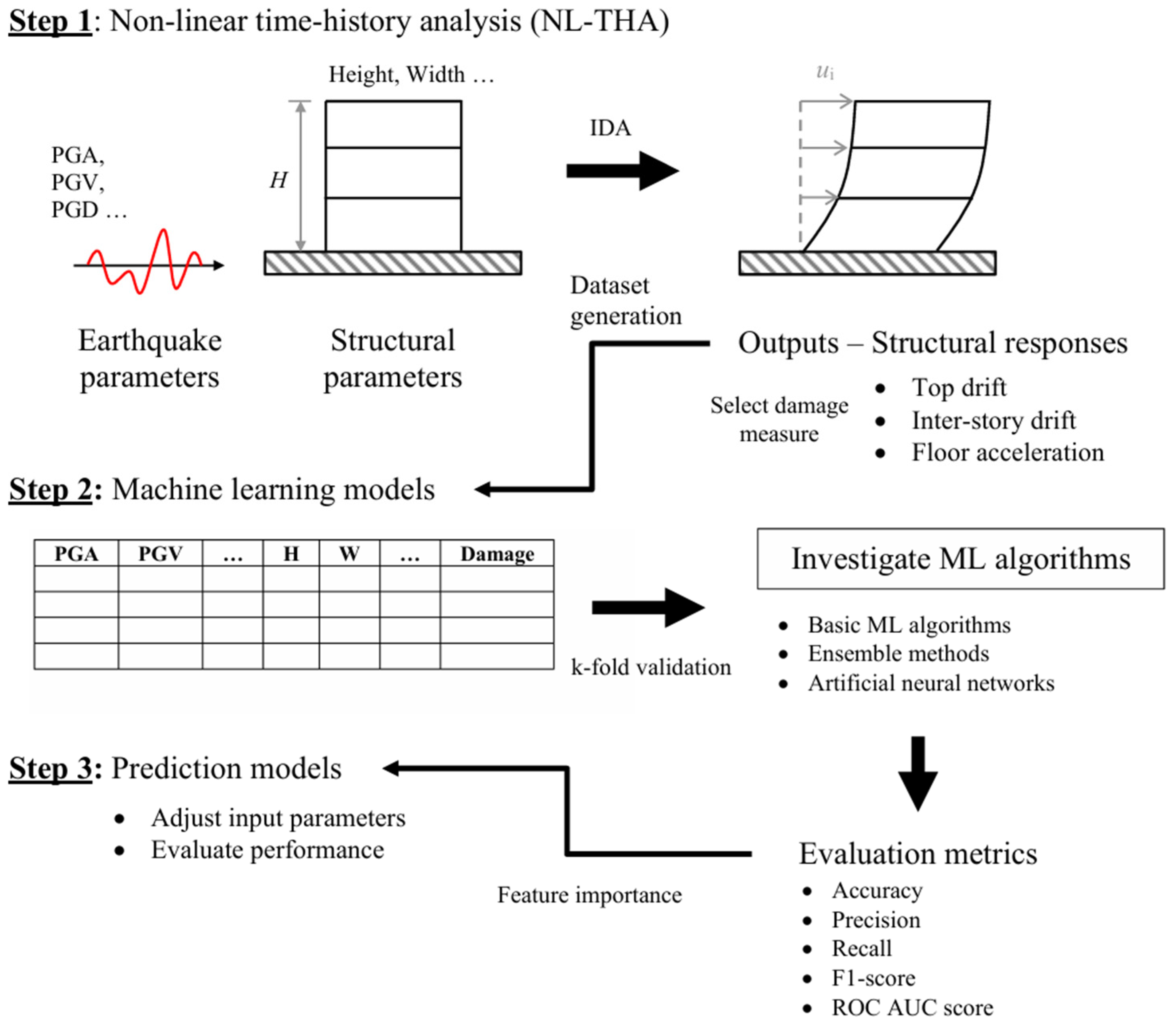
2. Methodology

To accomplish the project objectives, representative datasets and diverse ML algorithms were required. The training and testing datasets were first generated through IDA, which involved analyzing the structural responses and damage states of buildings with different structural and geometric properties under different levels of earthquakes via NLTHA [11]. The results were consolidated and presented in tabular format for ML model development. A variety of ML algorithms, such as basic algorithms, ensemble methods, and ANNs, were adopted and their effectiveness was evaluated. Figure 1 shows the flow chart of the methodology. Details of the non-linear analysis, ML models, and parameters are summarized in the following sections.

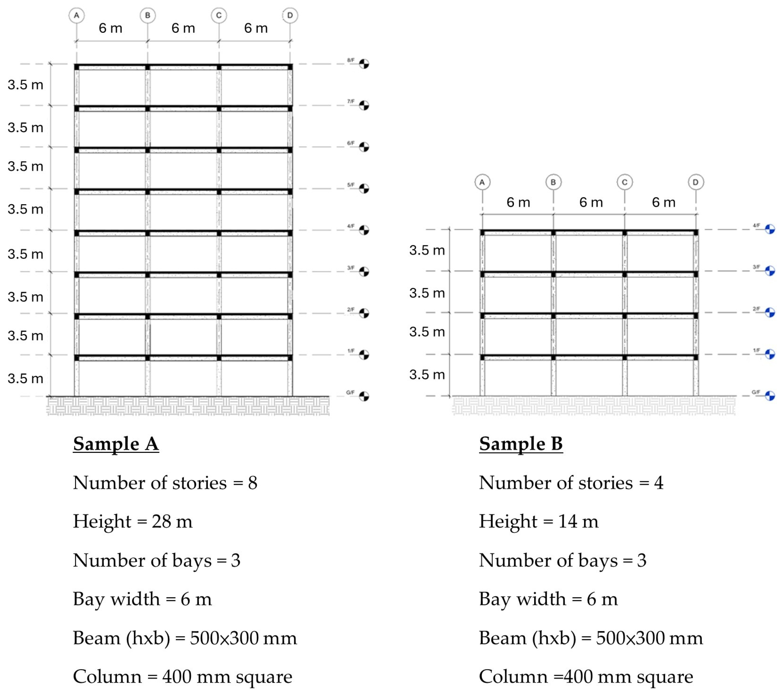
2.1. Building Models and Incremental Dynamic Analysis (IDA)

In total, 40 RC moment-resisting frames were developed in step 1 based on the code of practice in Hong Kong (HKCP2013) [46], which does not involve seismic-resistant design considerations. The dead load and imposed load were taken as 3.5 kN/m2 and 3.0 kN/m2, respectively. Some models were taken from previous studies [47,48]. Building models with overall height and width ranging from 14 m to 80 m and 18 m to 30 m were developed. The aspect ratio ranged from 0.778 to 4.276. Concrete grades C35, C45, and C50, with elastic modulus values of 23.7 kN/mm2, 26.4 kN/mm2, and 27.7 kN/mm2, respectively, were used in the design. The elastic modulus and yield strength of steel reinforcement were 200 kN/mm2 and 500 N/mm2, respectively. The steel ratio of beams ranged from 0.70% to 2.38%, while the steel ratio of columns ranged from 1.20% to 4.36%. Samples of 4- and 8-story buildings are shown in Figure 2. A variety of beam and column sizes were considered.
The building models were developed and analyzed using the finite element software ETABS, with the consideration of both material and geometric non-linearities. Material non-linearity was modeled using the lumped plasticity method, with FEMA356-defined plastic hinges assigned to member ends. Plastic hinge was modeled as an M3 hinge for beams, while a P-M2-M3 hinge was adopted for columns to take account for the coupled axial–flexural behavior. Geometric non-linearity was modeled by activating the second-order P-delta effects in the analysis setting.
All building models were first loaded by a dead load of 1.0 Gk and an imposed load of 0.3 Qk, where Gk and Qk are the dead and imposed loads, respectively. Second, NLTHA was performed to determine the seismic performance of buildings. Earthquake records are summarized in Table A1 in Appendix A. For each earthquake, the peak ground acceleration (PGA) was scaled from 0.1 g to 1.0 g for IDA. The simulation results were used to develop ML models.

2.2. Damage Class

There are several different ways to measure the damage levels of buildings or components, such as flexural damage ratio, the Park and Ang damage index, and the ratio between the final and initial vibration periods [2,49,50]. Table 2 lists some examples of damage indices in literature [48]. Among all damage indices, the maximum inter-story drift ratio (MIDR) was selected as the damage measure (DM) in this study. The MIDR is a widely used global indicator to assess damage levels of buildings in many international guidelines [4,5] and research [25,29].
The damage class of a building can be determined using predefined thresholds of the selected damage measure. According to FEMA356 [5], seismic performance levels are categorized into Immediate Occupancy (IO), Life Safety (LS), and Collapse Prevention (CP). According to HAZUS [53], damage states are categorized into five levels, including None Damage (ND), Slight Damage (SD), Moderate Damage (MD), Extensive Damage (ED), and Complete Damage (CD). In the current study, the damage level of buildings was defined with reference to a previous study [47], as shown in Table 3. The MIDRs of buildings with different structural and earthquake parameters were determined through numerous IDAs. Their performance was then categorized according to different damage levels (from 0 to 3) to train the supervised ML models for classification.

2.3. Machine Learning Algorithms

The application of a data-driven approach via ML was investigated in this study using the data that were generated via NLTHA in step 1. Five basic ML algorithms, namely logistic regression, support vector machine, K-nearest neighbor, decision tree, and Gaussian Naïve Bayes, were used. Four ensemble methods, namely voting, stacking, bagging, and boosting methods, were adopted. In addition, artificial neural networks were explored to evaluate their effectiveness in damage classification. The performance of the selected ML algorithms was evaluated and compared, which will be discussed later. Most of these basic and ensemble algorithms are available in a powerful ML tool in python version 3.11 called scikit-learn library [54]. Moreover, neural network-based models can be developed using the libraries tensorflow and keras. The python library optuna was used with minor adjustments to set the hyper-parameters for the basic and ensemble ML algorithms [55]. The hyper-parameters of interest were first selected, and then, the optuna library was used to search for the most suitable values by optimizing the loss based on the scores obtained using cross-validation. The Tree-structured Parzen Estimator algorithm was used for the sampler. The number of trials was set as 100 in this study. The ranges of hyper-parameters considered in tuning are presented in Appendix B. The hyper-parameters adopted for each ML model are summarized in Table 4. The following paragraphs roughly summarize the basic characteristics of the ML algorithms adopted in this study [23,48].

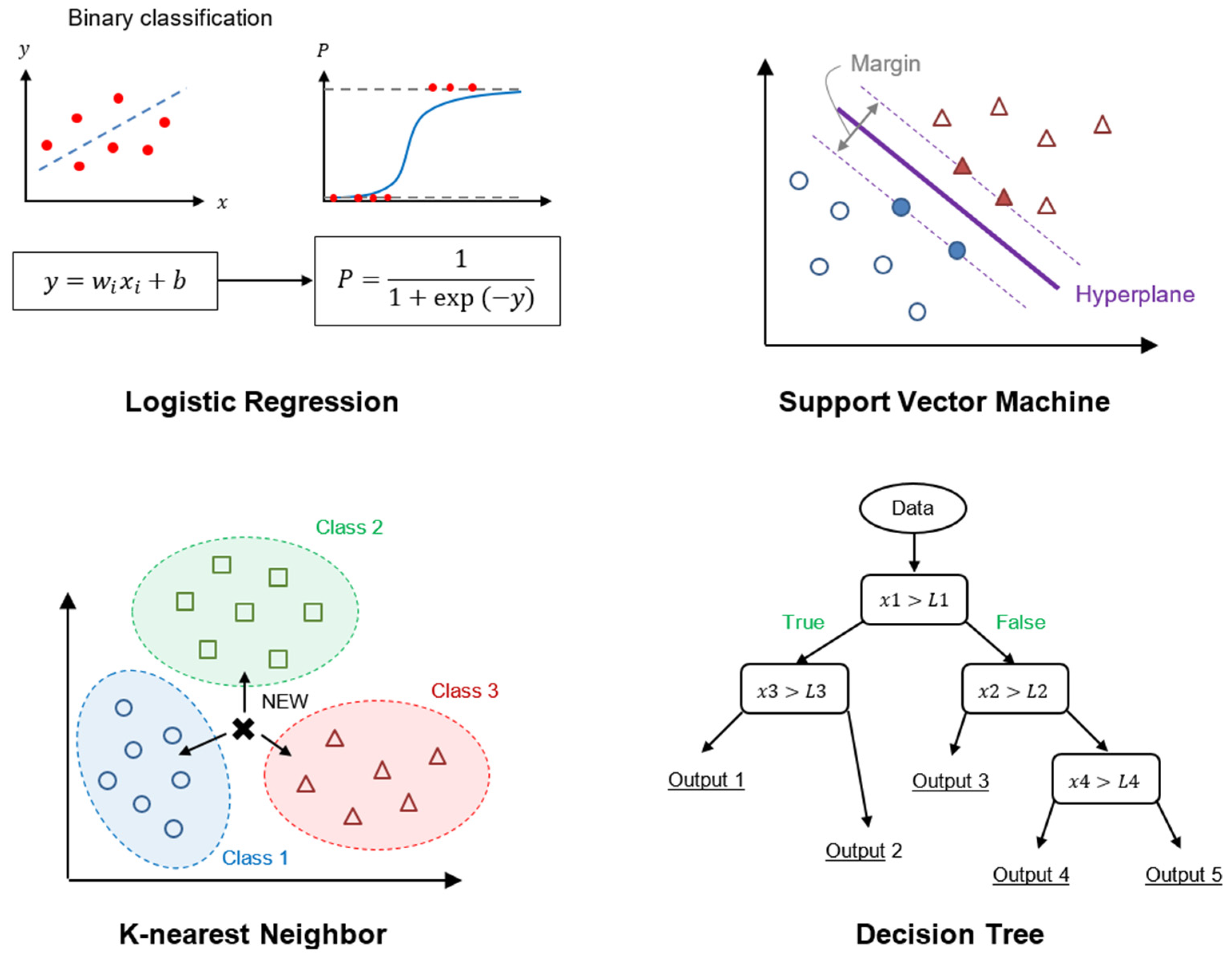
2.3.1. Basic Machine Learning Algorithms

Machine learning offers a diverse range of algorithms for regression or classification, each founded on distinct mathematical theorems and assumptions. The effectiveness of different algorithms depends on the problem context, making ML algorithm selection to often rely on experience or iterative experimentation. Figure 3 illustrates the major characteristics of five basic ML algorithms.
Logistic regression (LR) is a typical linear model for classification problems [56]. For problems with K-classes, the probability of the target being class k can be expressed as
p k ( X i ) = e x p ( X i W k + W o , k ) l = 0 k 1 e x p ( X i W l + W o , l ) ,
where X i is the feature array, while W k and W o , k are the coefficients (weight and bias) that can be determined by minimizing the cost function. In general, this algorithm works very well if the dataset is linearly separable.
Support vector machine (SVM) is a powerful ML algorithm for regression and classification [57]. This method identifies optimal hyperplanes for classifying data into different classes by maximizing the margin, expressed as 2 / w , which represents the distance between the hyperplane and the data points, where w is the length of the coefficient vector w . The slack variable ζ k 0 is added for classifying non-linearly separable problems. For classification problems, SVM is equivalent to optimization problems, written as
min w , b , ζ 1 2 w T w + c i = 1 n ζ i
and subjected to a constraint, written as y i b + w T x i 1 ζ i , where x i is the training feature vector, y i is either equal to 1 or −1, and c is a factor used to control the penalty for misclassification. SVM can be extended to non-linear classification problems via kernel methods. These methods employ mapping functions (e.g., polynomial, radial basis functions) to transform non-linearly separable data into a higher-dimensional space where linear separation becomes possible. SVM normally performs very well for both separable and non-separable datasets.
Nearest neighbors is an instance-based algorithm in which ML models are constructed by memorizing the training data rather than directly training a function with coefficients. This approach relies on the spatial distribution and distance metrics of the datasets. One widely used algorithm is the K-nearest neighbor (KNN) [58]. In this case, a pre-defined integer k is selected by the user. The training data are divided into k-classes based on their spatial distribution. Given a new data point, the distances between this new data and the labeled datasets are calculated. The new point can be classified based on the computed distances following a plurality vote of its neighbors. Another nearest neighbor method is radius-based neighbors. In this approach, users need to pre-define a fixed radius rather than pre-defining the numbers of classes.
Decision tree (DT) is a non-parametric algorithm that uses a hierarchical tree structure for decision making [59]. The tree is composed of nodes presenting different decisions. During construction, information gain, which can be calculated based on the probabilities of occurrence, and impurity measures of the training data are computed. Commonly used impurity measures include Gini impurity, entropy, and log loss. By tracing all possibilities under consideration, all new data can be classified into existing groups. A key advantage of decision trees is their interpretability, where the model can be presented as a tree diagram to illustrate the decision logic.
Naïve Bayes (NB) is a classical ML algorithm used for classification exercises based on probability theory. In this algorithm, the conditional probabilities of input features belonging to each class are computed. The results are then used to evaluate the probability of all classes for prediction purposes. The Gaussian Naïve Bayes algorithm assumes that all input features follow a Gaussian distribution.

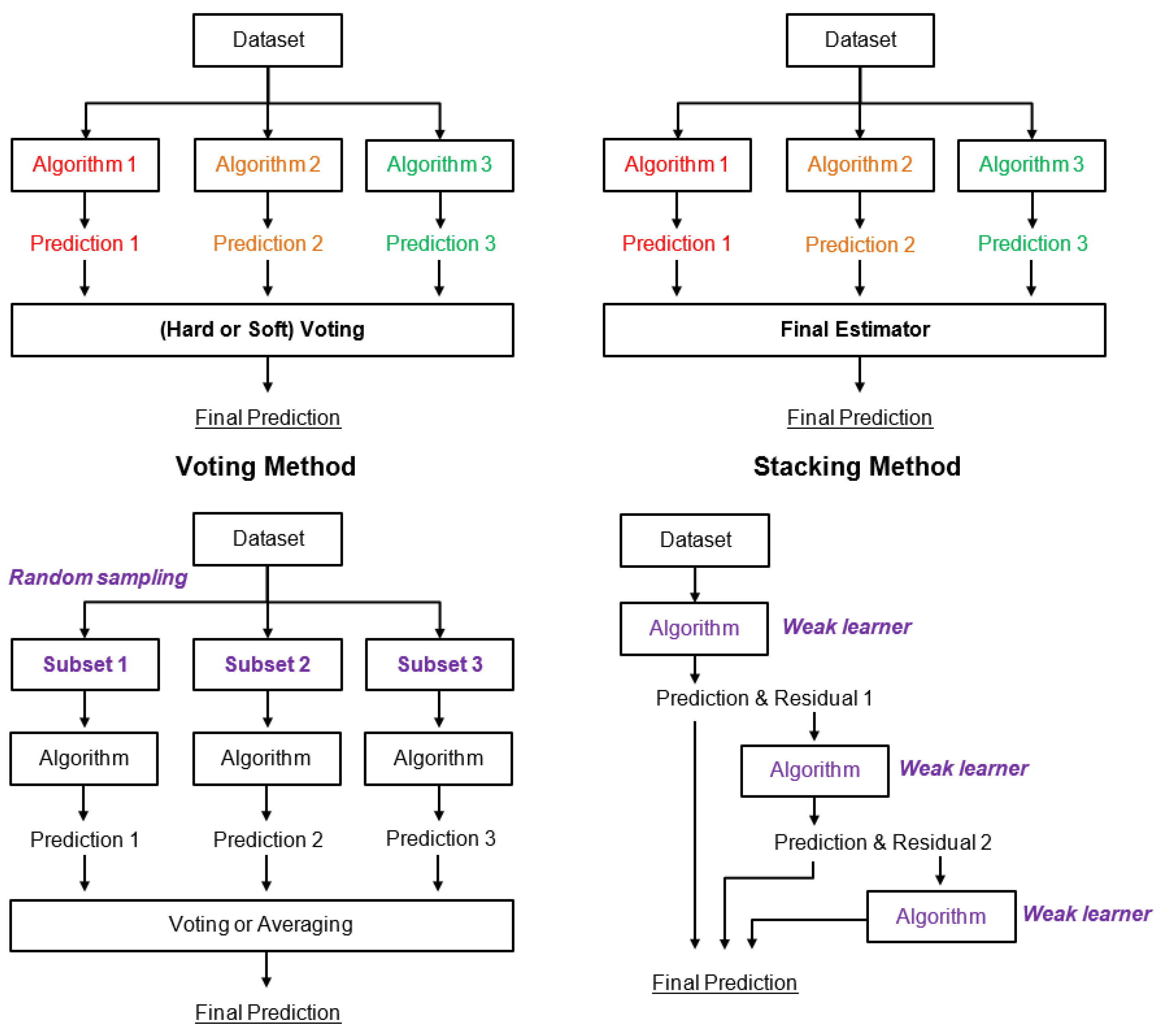
2.3.2. Ensemble Methods

The ensemble method combines multiple ML models together to enhance the overall performance and generalizability. Each ML model can work in parallel with the other models. The final predictions are obtained by combining the results of each model together via a suitable method. Moreover, ensemble models can be built by combining ML models sequentially to reduce the residuals from previous models. Figure 4 presents the general architecture of the selected ensemble methods used in this study. Their basic characteristics are summarized in the following paragraphs.
The voting method provides an effective way to combine multiple ML models to improve the predictive performance. This method utilizes the selected ML algorithms as base estimators, each generating independent predictions from the training dataset. The final prediction can be determined using either a majority vote (hard voting) or weighted average probability (soft voting). Averaging the predictions from different ML models can minimize the weaknesses of each individual ML model. In the current study, several basic classifiers and ensemble models were selected as base estimators. Soft voting was used to compute the final prediction.
The stacking method employs a two-stage learning process to improve the overall performance [60]. First, several base learners are trained independently using the training dataset to generate preliminary predictions. Second, a final estimator, which is called the meta-learner, is trained by taking the preliminary predictions as inputs. This hierarchical two-stage process allows the meta-learner to capture and leverage the complementary strengths of the diverse base models. In this study, basic and ensemble models served as base estimators, while the logistic regression classifier was selected as the meta-learner.
The bagging method improves model robustness by training multiple models with the same ML algorithm on different randomly sampled data subsets. Each subset, which is generated through random sampling, trains an independent classifier. The final prediction can be obtained by combining the predictions from different classifiers. This method can help to reduce the over-fitting of ML models. A famous example is random forest (RF), which applies the bagging method to decision trees [61]. RF typically outperforms simple decision trees but involves a higher computational effort. In this study, random forest and two bagging models with support vector machine and extra-trees classifier as the base learners were considered.
The boosting method is a special ensemble method that uses several weak learners to enhance the models’ accuracy. In this method, all learners are trained sequentially to handle the residuals of previous learners. The basic concept of boosting algorithms is illustrated in Figure 4. For example, adaptive boosting (AdaBoost) assigns weights to each data point, and wrongly classified data will be assigned higher weights for training the next weak learner [62]. By repeating the process through training, many weaker learners in sequence could help to improve prediction, which can be achieved by combining the results of weak learners via majority voting.
On the other hand, gradient boosting trains models in sequence using the gradients of the loss function (residuals) to minimize the loss in new models. The final prediction can be obtained using an additive calculation,
F m x = F m 1 x + β m h m ( x )
where F m 1 x is the results from previous models, and β m is the weight of the m-th weak learner, h m ( x ) . Gradient boosting decision tree (GBDT) [63], eXtremely gradient boosting (XGBoost) [64], and light gradient boosting machine (LightGBM) [65], are examples of gradient-based boosting algorithms with decision trees as weaker learners. Both adaptive and gradient boosting methods were explored in this study.

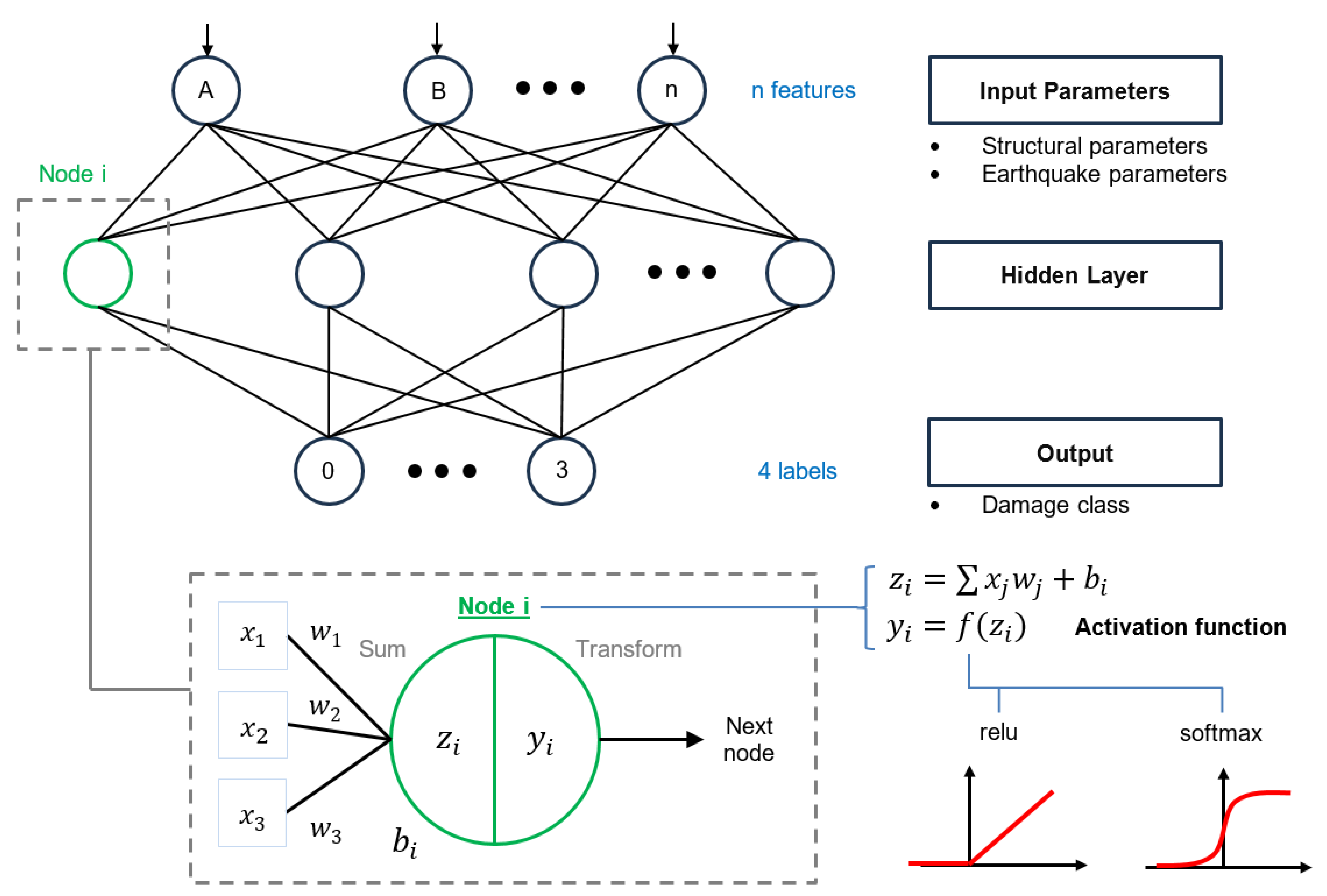
2.3.3. Artificial Neural Networks (ANNs)

Recently, ANNs and their relevant algorithms have been successfully applied to different real-life problems. A vanilla ANN model consists of layers that are composed of nodes [66]. The number of layers and nodes depends on the problem. Each node processes inputs x i from the previous layer via weights w i and bias b i . The result is then passed through an activation function to introduce non-linearity in the system, written as
y i = f w i x i + b i ,
where the output y i can be continuous or discrete values, depending on the nature of the problem. Figure 5 shows a simple neural network architecture with one input layer, one output layer, and one hidden layer in the middle. The optimal values of weights and bias can be determined via training using the input and output datasets with a backpropagation algorithm [67]. Deep learning methods use ANNs with many hidden layers to extract important features from the original dataset. Examples of deep learning include convolutional neural networks and recurrent neural networks. The former is a famous ML algorithm in the field of computer visuals, while the latter is an efficient algorithm for processing sequential data, such as time-series data and text data.
In this study, ANN models were developed based on multi-layer perceptron (MLP), which is also called a feedforward neural network. Three different network architectures, with one, two, and three hidden layers, were explored to assess the capability of each architecture in classification problems. The Relu function was used as the activation function for most of the units, with the exception that softmax function was adopted for the last layer to convert the results to probabilities. Dropout layers with a dropout rate of 0.2 were used for dense layers to control over-fitting issues. The output parameter was the damage levels, which is modeled using one-hot vector. The epochs and batch sizes were taken as 150 and 16, respectively, during the training of the ANN models.
In addition to the classic ANN discussed above, stacking and gradient boosting techniques were also employed to investigate the effects of ensemble techniques on the ANNs. For the stacking method, five ANN models were trained using datasets that were randomly selected from the original training dataset. After that, the predictions from individual ANN models were consolidated, as shown in Figure 6. The results were then used for training the meta-learner. Logistic regression classifier was adopted as the meta-learner in this study. For the gradient boosting method, the algorithm used was similar to the GBDT mentioned above, with the exception that an ANN was adopted as the weaker learner rather than a decision tree [68].

2.4. Data Consolidation

In supervised learning, input parameters (features) and output parameters (label or target) are required for training the ML models. In the study, input parameters were divided into earthquake parameters and structural parameters. Instead of considering the ground motion histories, earthquake parameters were used to represent the major characteristics of an earthquake. Some studies have considered a variety of earthquake parameters as input features [36,69]. In total, 15 earthquake parameters were considered, including peak ground acceleration (PGA), peak ground velocity (PGV), peak ground displacement (PGD), spectral acceleration at 1.0 s (Sa1), spectral acceleration in the fundamental period of the building (Sa(T1)), acceleration spectrum intensity (ASI), Housner intensity (HI), displacement spectrum intensity (DSI), PGV/PGA, Arias intensity (Ia), mean period (Tm), predominant period (Tp), significant period (Ts), specific energy density (SED), and resonant area (A1). The earthquake parameters and their definitions adopted in this study are summarized in Table 5.
Structural parameters are used to represent structural properties. In total, 18 structural parameters were considered in this study, including the number of bays, bay width, width of building (W), number of stories, total height of building (H), structural aspect ratio (H/W), maximum axial load level (vd), moments of inertia of beam and column (Ib and Ic), moment resistances of beam and column (Mb and Mc), steel reinforcement ratios of beam and column ( ρ s b and ρ s c ), fundamental periods for mode 1 to 4 (T1 to T4), and story stiffness (K). Moments of inertia are computed based on the dimension of beams and columns. Moments of resistance of members are determined in the ETABS models. The maximum axial load level is calculated as
v d = N f c u A c ,
where N is the maximum axial force at columns determined by NLTHA, fcu is the concrete strength, and Ac is the column’s area. The steel reinforcement ratio depends on the reinforcement provided in the members. The four modal periods are obtained from the modal analysis in ETABS. Story stiffness is determined based on the approximate method of analysis for a rigid frame [70], expressed by
K = 12 E h 2 1 B + 1 C ,
where E is the elastic modulus, B = I b / L , C = I c / h , L is the beam length, and h is the column height. In addition, the influences of different input parameters were investigated. The structural parameters are summarized in Table 6.
The output parameters are the expected results that will be generated by the ML models. For the purpose of damage classification, the damage class was selected as the output parameter. In this study, the damage class of a building was defined based on the MIDR from NLTHA (Table 3).

2.5. Data Preprocessing

Before training the ML models, pre-processing the training and testing datasets should be carried out to improve the models’ accuracy and convergence. The input features x i are typically normalized or standardized before training since some ML algorithms are sensitive to the magnitude of the input features. In this study, the min–max normalization technique was adopted to convert the data to a range between 0 and 1 using the following equation:
x i n o r = x i   x m i n x m a x   x m i n
where x i is the i-th feature and x m i n and x m a x are the minimum and maximum values of the i-th feature. This conversion can be performed by using the method MinMaxScaler in the scikit-learn pre-processing package.

2.6. Training and Testing

During training and testing, the k-fold cross-validation method was adopted, where k = 5. This method is commonly used to assess the performance of ML algorithms and to obtain less biased results. In this case, the entire dataset was divided into 5 subsets. Four subsets were used for training the ML models and the remaining subset was used for testing the performance of the ML models. This process continued until all subsets were used for both training and testing. The labeled output y i contained discrete values (0, 1, 2, 3) representing the damage level of buildings. The output data were converted using the one-hot encoding technique when the ANN algorithm was under consideration. In this study, the number of samples for each damage class [0, 1, 2, 3] were [1907, 1843, 1273, 457]. More samples belong to damage levels 0 and 1 since the buildings had a satisfactory performance under the considered levels of earthquakes.

3. Data Analysis and Discussion

3.1. Performance of ML Models for Damage Classification

ML models for the damage classification of RC buildings were developed using the dataset described in the previous sections. Different approaches, including the basic ML algorithms, ensemble methods, and ANN models, were considered. This section presents the models developed using all input features. The performance of each ML model for the damage classification of buildings under earthquakes was evaluated using four commonly used evaluation metrics for classification problems, including accuracy, precision, recall, and F1-score. They are defined as follows:
A c c u r a c y = T P + T N T P + T N + F P + F N ,
P r e c i s i o n = T P T P + F P ,
R e c a l l = T P T P + F N ,
F 1 = 2 T P 2 T P + F P + F N
where TP, TN, FP, and FN represent true positive, true negative, false positive, and false negative, respectively. In addition, the values of the computer area under the receiver operating characteristic curve (ROC AUC score) are also provided.
Figure 7 presents the confusion matrices for the four selected ML models with good performance, namely SVM, RF, XGBoost, and ANN. Note that the confusion matrices in the figure are evaluated by summing up the matrices obtained in each fold during the k-fold validation process. A confusion matrix is helpful to evaluate the predictability of a particular ML model for each class (or damage level, as shown in Table 3). Table 3 summarizes the predictions from the models and the actual values. The value inside each box represents the number of predictions for a damage class. The diagonal elements in the confusion matrix represent correct prediction. The results show that the majority of the predictions are correct for all damage levels. This indicates that the four selected ML models have adequate capacity to classify the damage levels of RC buildings.
Figure 8 shows the overall ROC curves and the ROC curves for each damage class for the four selected models. The ROC curve, which is a plot of the true positive rate against the false positive rate, is also an effective indicator to assess the performance of ML models. The results illustrate that all ROC curves are far above the diagonal line (i.e., random guess), indicating that the performance of the selected models is good.

3.1.1. Performance of Basic Models

The overall performance, including accuracy, precision, recall, F1-score, and ROC AUC score, of all ML algorithms under consideration is summarized in Table 7. Macro average is used to evaluate the overall performance instead of the individual damage level. Among all five basic ML models, SVM performs the best in all evaluation metrics, with accuracy equal to 86.5%, followed by DT, except for precision and ROC AUC score. The accuracy of decision tree is 82%. The performance of KNN is comparable to LR, with accuracy between 80.1% and 80.4%. Similar trends were found for recall and F1-score. In contrast, the ROC AUC score of DT is the lowest among all basic ML models. The accuracy of the Gaussian Naïve Bayes algorithm is 69.7%, which is about 10% lower than that of the other basic ML algorithms. In general, all basic models have good accuracy, with values approximately equal to 80%, except for the Naïve Bayes algorithm. The results of the basic algorithms can serve as reference for comparing ensemble methods and the ANN.

3.1.2. Performance of Ensemble Models

The overall performance of ensemble methods is generally great, as most of the evaluation metrics are larger than 85%, as shown in Table 7. In general, the results show that three boosting methods, including GBDT, XGBoost, and LightGBM, outperform the basic methods in this problem. In particular, XGBoost performs the best among all boosting models in all metrics, with accuracy of 89.1%. LightGBM performs slightly better than GBDT, with accuracies of 88.1% and 87.7% for LightGBM and GBDT, respectively. Similar trends are observed in the other metrics. The excellent performance of the boosting methods indicates that introducing weak learners sequentially can significantly help to improve the models’ overall performance.
In addition to boosting methods, bagging methods, which train several classifiers using datasets that are extracted randomly from the original dataset and then combine the predictions together as the final outputs, are also effective in enhancing the models’ overall performance. Table 7 shows that RF performs better than the other two bagging models and the basic models in all metrics. It achieves an accuracy of 88%, which is comparable to that of most boosting models. On the other hand, the bagging model with the extra-trees classifier as the estimator performs slightly better than the bagging model with SVM as the estimator, particularly in terms of recall and F1-score.
Voting and stacking methods are developed by combining several base estimators together in parallel and generating the final outputs using different mechanisms. Voting methods generate the final outputs from the predictions of base estimators using soft voting or the majority rule. In this study, two voting models with two different sets of base estimators, involving four basic models (LR, SVM, DT, and KNN) and three ensemble models (RF, XGBoost, and GBDT), were considered. Soft voting was adopted to produce the final outputs. It was observed that neither voting models showed significant improvement in the final prediction. This may be due to the fact that the performance of their base estimators was not uniform, with some models outperforming others.
The stacking method introduces a final estimator to generate the final output. Two stacking models with two different sets of base estimators, involving the four basic models (LR, SVM, DT, and KNN) and three ML ensemble models (RF, XGBoost, and GBDT), were investigated. The logistic regression classifier was selected as the final estimator for both stacking models in this study. Different from our expectation, the results show that neither stacking models show significant improvement in their overall performance compared with their base learners. This may be due to the selection of the ML algorithm for the final estimator. Other effective ML algorithms, such as SVM, may be used as an alternative.

3.1.3. Performance of ANN Models

The performance of ANN models depends on the network’s architecture, such as the number of units, number of layers, and layer properties. In this study, ANN models constructed based on MLP with one hidden layer, two hidden layers, and three hidden layers were investigated. Note that large numbers of units and layers may significantly increase the computational effort and possibly lead to over-fitting issues.
The results show that the ANN model with three hidden layers and 128 units (ANN-5) performs the best among all ANN models. It achieves accuracy of 87.2%, which is slightly lower than that of ensemble methods in this classification problem. Similar trends were found for the other metrics. In general, the accuracy of ANN models is around 86% to 87%, regardless of the number of layers and units. Increasing the numbers of layers and units cannot always improve the models’ overall performance.
This study also explores the use of stacking and boosting techniques for ANN models. For the stacking ANN model, five ANN models with two hidden layers and 128 units per layer were trained separately using the training dataset. The results from each ANN model were then concatenated as the input for training an LR meta-learner. The results show that the stacking techniques can slightly improve the overall performance of ANN models. The accuracy of the stacking ANN model is about 1% better than that of the ANN models with two hidden layers. The performance of the gradient boosting ANN model is similar to that of the stacking ANN model. The results reveal that ANN models are capable of resolving classification problems. However, they normally need longer training times and more advanced knowledge in ML model development. Therefore, to handle tabular data, using tree-based ensemble models, such as XGBoost and RF, can achieve high accuracy with limited computational efforts for model development.
Simple comparisons of past works are valuable to understand the performance level of the ML models in this study. ML models in [32] were developed for predicting the damage class (class 0 to 2) of three selected RC structures based on DT, linear discriminant analysis, NB, SVM, and KNN. The results revealed that KNN performed the best, with an accuracy of 93.6%. The study in [33] developed ML models for classifying damage into five levels using XGBoost, RF, and active learning model. The best model was active learning, with an average accuracy of 84% for testing dataset, while the accuracy of XGBoost was 80%. The ML model comparison in [34] considered a total of 18 classifiers, and SVM with Gaussian kernel outperformed the others, with accuracies of 88.5% and 91.1% after fine tuning. Despite differences in training datasets and output labels compared to the previous studies, the ML models developed in this study, such as XGBoost with an accuracy of 89.1%, can achieve satisfactory performance in damage classification. The results further indicate that ANN models with ensemble techniques, such as gradient boosting ANN, can achieve accuracy comparable to efficient algorithms, like RF and SVM. ANNs offer the advantage of flexibility, allowing the model to incorporate multiple complex input features, such as time-series data and images, for future development.

3.2. Feature Importance

In the previous section, the performances of different ML models with extensive input parameters were assessed and compared in detail. However, ML models with too many input parameters with low correlations may affect the final predictions. Moreover, ML models with too many inputs will increase the difficulty of applying them for the rapid damage assessment of buildings. Hence, ML models can be further improved by optimizing the numbers of input parameters. The effectiveness of input parameters can be studied via feature importance and SHAP values.
The importance of input parameters depends on the ML algorithms. Two ensemble models with good performance, namely XGBoost and RF, were considered. Figure 9a,b present the impurity-based feature importance of input parameters in the ML models. For earthquake parameters, the specific energy density (SED) contributes the most in XGBoost. In addition, the influences of the other velocity-related earthquake parameters, such as peak ground velocity (PGV) and Housner intensity (HI), are also significant. However, the contribution of the widely used parameter, peak ground acceleration (PGA), is not very high in XGBoost. For RF, in addition to velocity-related parameters, spectral acceleration (Sa(T1)), displacement spectrum intensity (DSI), and resonance area (A1) are highly important for the models’ predictions.
The importance of structural parameters in the two prediction models varies. In XGBoost, the width of buildings is the most important structural parameter, followed by the moment of inertia of each column (Ic) and the first-mode vibration period (T1). The height of buildings (H) is another important structural parameter in this model. On the other hand, the maximum axial load level (vd) is the most important structural parameter in RF, followed by the first-mode vibration period and the height of buildings. In short, the building’s geometry and first-mode vibration period are generally important in both prediction models.
SHAP values are effective indicators to reflect the contributions of each input feature to the predictions of the ML models. Figure 10 and Figure 11 present the SHAP values for each damage class of XGBoost and RF, respectively, with the damage classes defined in Table 3. Only the best 20 features are shown in the figures. The color of each dot in the figure reflects the value of the parameter. A positive SHAP value indicates that the parameter has a positive impact on the model output.
For the earthquake parameters, spectral acceleration in the fundamental period (Sa(T1)) significantly affects the final predictions in both models. In XGBoost, low values of Sa(T1) tend to have positive contributions to lower damage classes (0 and 1), while high values of Sa(T1) tend to result in higher damage classes (2 and 3). Similar observations were found for parameters such as PGV, HI, SED, and DSI. The trend for PGD is similar, but the impact values are smaller. The impacts of ASI are not very clear, since the SHAP values are generally small and have no unique patterns. The impacts of these parameters (Sa(T1), PGV, HI, SED, and DSI) are similar in RF. Moreover, the parameters V/A and ASI show the same trend, whereby high values of these parameters are favorable in predicting higher damage classes.
The contributions of structural parameters are quite diversified in different damage classes. In XGBoost, the first-mode vibration period T1 and axial load level vd are important parameters that influence predictions. Lower values of these parameters tend to make a high contribution to damage class 0, while high values have a high contribution to damage classes 2 and 3. Height has certain impacts on the predictions. Large height values have positive impacts on damage class 0, while low height values have certain impacts on damage class 2. Another potential parameter is the width of buildings. Low values have a positive impact on damage class 0, while high values tend to be favorable for higher damage classes. The moment of inertia of each column has certain impacts on predictions, except for damage class 3. The other structural parameters, such as moment resistances of members, contribute to certain damage classes but not all. In RF, the trends of T1 and vd are similar to those in XGBoost, but the contributions are lower. The trends of height and width are also similar in general, but the contributions are higher in RF.
In short, SHAP values provide valuable insights to identify significant features of the prediction models. After that, physical interpretations of key features to the buildings’ performance can be explored. Among all earthquake parameters, the specific energy density (SED) is a key parameter influencing the predictions in this study. This is because earthquakes with a high SED typically result in more significant structural responses due to high energy inputs, thereby causing severe damage to buildings. In addition to SED, spectral acceleration Sa(T1) is also significant since this parameter directly reflects the maximum earthquake-induced accelerations (and forces) on the structures. Higher values of Sa(T1) increase seismic forces, leading to a greater structural response. Among all structural parameters, building geometry, such as building width, can influence predictions, but the relationship is not always simple. This is because the building width is related to the mass of buildings. This affects both the seismic forces and dynamic properties of buildings (e.g., natural periods of vibration), leading to variations in seismic responses.

3.3. Prediction Models with Reduced Parameters

For practical applications, the number of input parameters for the prediction models should be optimized such that the selected parameters should make a significant contribution to the prediction task but should not be too excessive so as to avoid inconvenient applications. In light of this, simplified prediction models for the preliminary damage classification of buildings were developed using reduced input parameters.
In the previous section, important features that significantly affect the models’ performance were identified, and hence, representative parameters can be selected with reference to the previous results. In addition, the selected parameters should be able to be obtained in practice. In view of feature importance and data availability, the earthquake parameters were reduced to PGA, PGV, PGD, Sa(T1), and V/A, while the structural parameters included height and width of buildings, maximum axial load level (vd), moment of inertia of each column, and first-mode vibration period. Only effective ML models were considered. The performance of the modified models is shown in Table 8.
The results indicate that most of the ML models maintain a similar performance level when the input parameters are optimized. For basic model, SVM performs similarly to the SVM model with a full set of input parameters. SVM generally performs lower than the ensemble models, except GBDT. XGBoost performs the best among all the methods under consideration, followed by AdaBoost. XGBoost achieves an accuracy of 88.2%, which is about 0.9% lower than that of the model with a full set of input parameters. The precision of AdaBoost is similar to that of XGBoost, but the other metrics are slightly lower. RF and LightGBM can also achieve satisfactory performance when the optimized input features are used. GBDT reaches an accuracy of 86%, which is slightly lower than that of the other ensemble models under consideration. Similar trends are observed for the other evaluation metrics. On the other hand, the average accuracy of ANN models is around 86–87%, which is slightly lower than that of the ensemble methods, such as RF and AdaBoost. Several neural network configurations were considered. The results show that increases in the number of layers cannot significantly enhance the models’ performance. The model with two hidden layers is generally sufficient in this problem. Ensemble techniques, such as stacking and boosting methods, can slightly enhance the models’ performance by reducing the computational time. However, the performance is still lower than that of XGBoost.

4. Conclusions

This study investigated the feasibility of using ML models for classifying the damage levels of RC buildings during earthquakes. Building models were designed without seismic consideration. Numerous NLTHAs were conducted to generate the dataset for training and testing the ML models. Representative earthquake and structural parameters were selected as the input features, while the damage level defined according to the MIDR was adopted as the output for ML model development through supervised learning. The performance and effectiveness of the selected ML algorithms, including five basic algorithms, four ensemble methods, and ANNs, were studied using suitable evaluation metrics, which were computed based on the k-fold validation method. The importance of different earthquakes and structural parameters was evaluated.
The results reveal that ML models can serve as an alternative method for a rapid vulnerability assessment of typical RC buildings instead of using the time-consuming NLTHA. This can be beneficial, particularly for vulnerability assessments of buildings at a regional scale. The major findings of this study are summarized below:
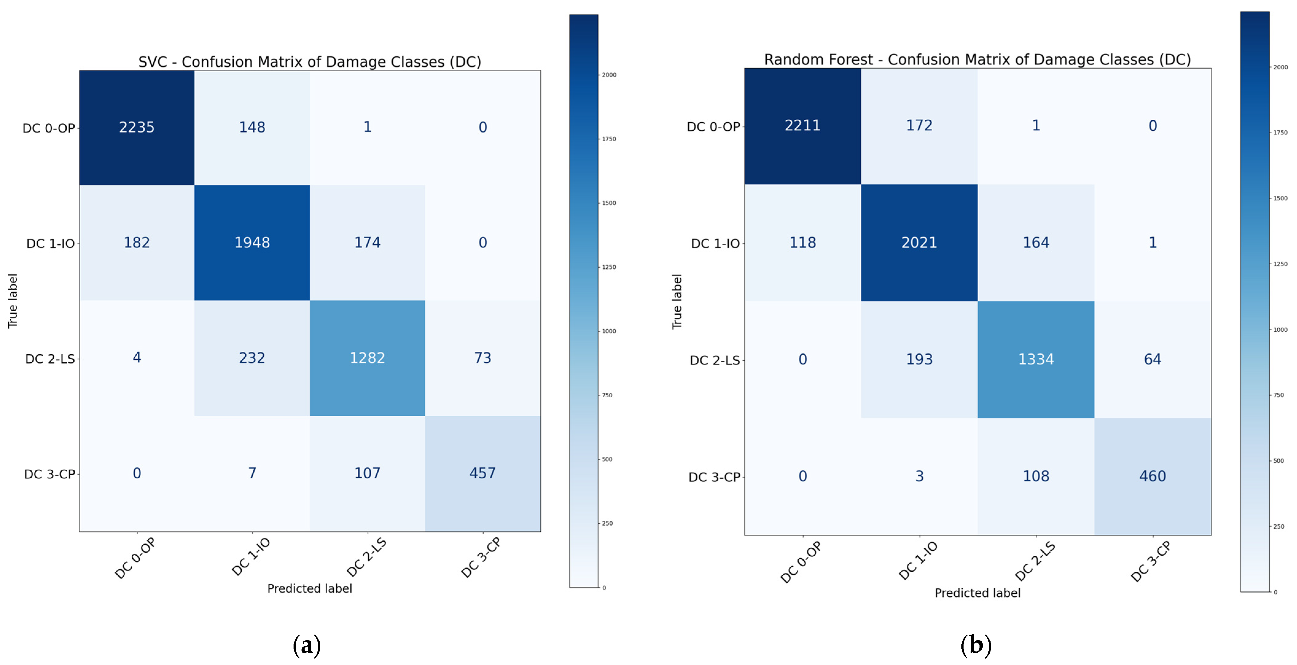
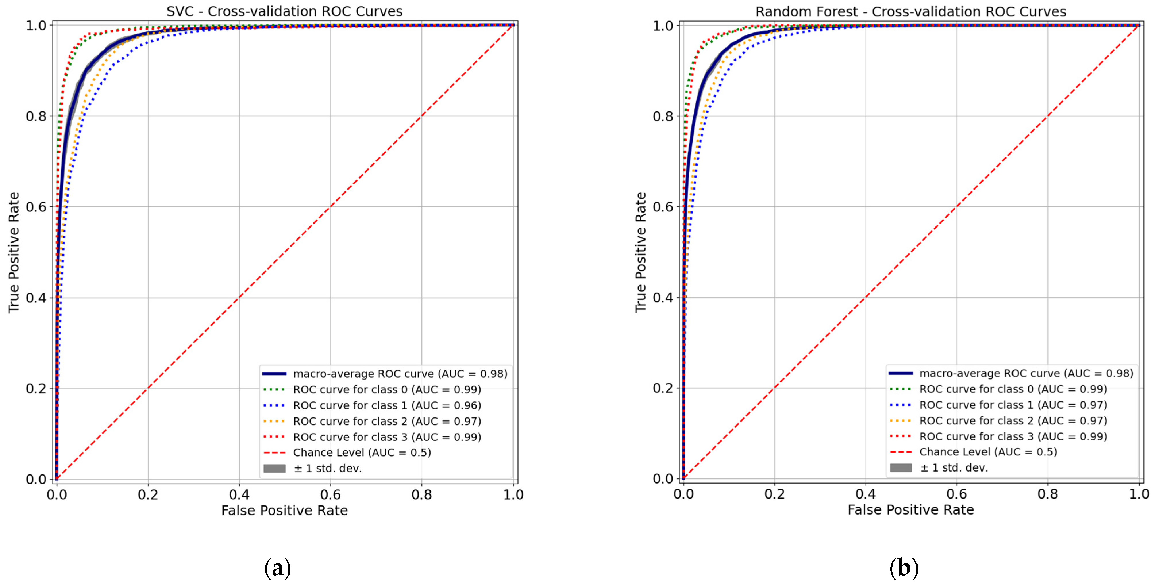
  • Among the five basic ML algorithms under consideration, SVM outperformed the other four basic algorithms in damage level classification. The performance of SVM is generally lower than that of the ensemble methods.
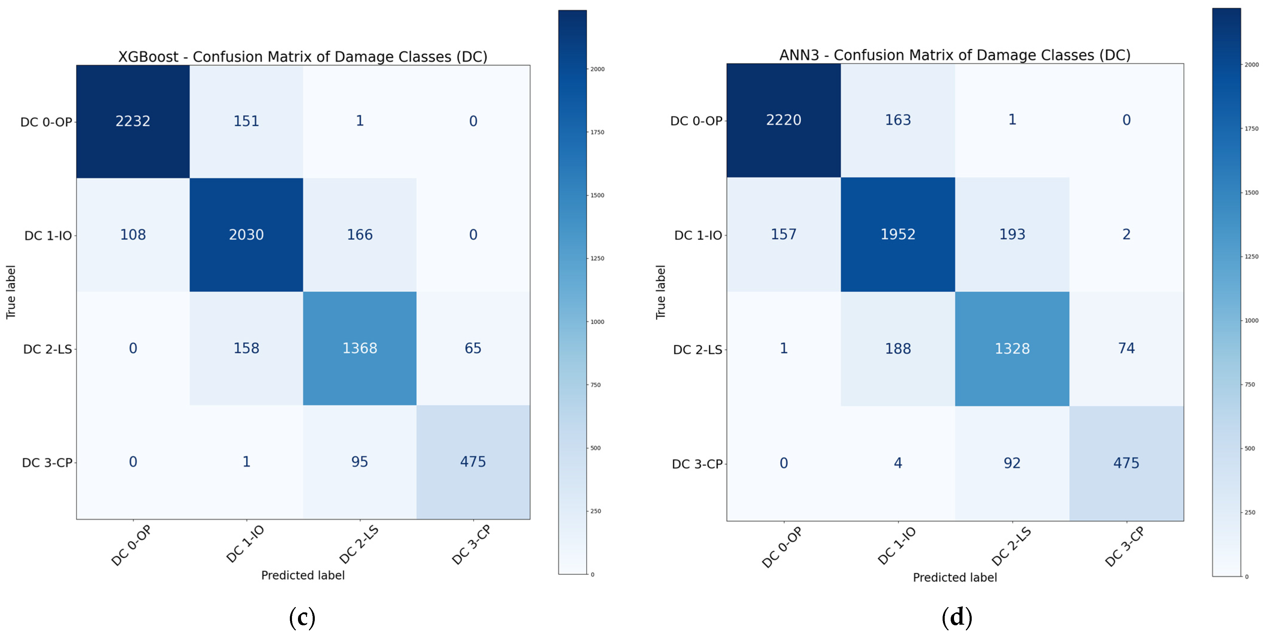
  • The performance of ensemble methods was generally better than that of the basic ML algorithms. Boosting and bagging methods, particularly XGBoost and RF, were the two most effective ML algorithms and could achieve high evaluation metrics in classification tasks. On the other hand, voting and stacking methods could not always enhance the overall performance of ML models.
  • ANN models were suitable for damage classification, with their performance comparable to many ensemble models. In this study, ANN models with two to three hidden layers were generally sufficient to achieve a good balance between accuracy and computation effort for classification. Further increasing the number of hidden layers cannot improve the models’ accuracy. The overall performance of ANN models could be enhanced by using stacking and boosting methods.
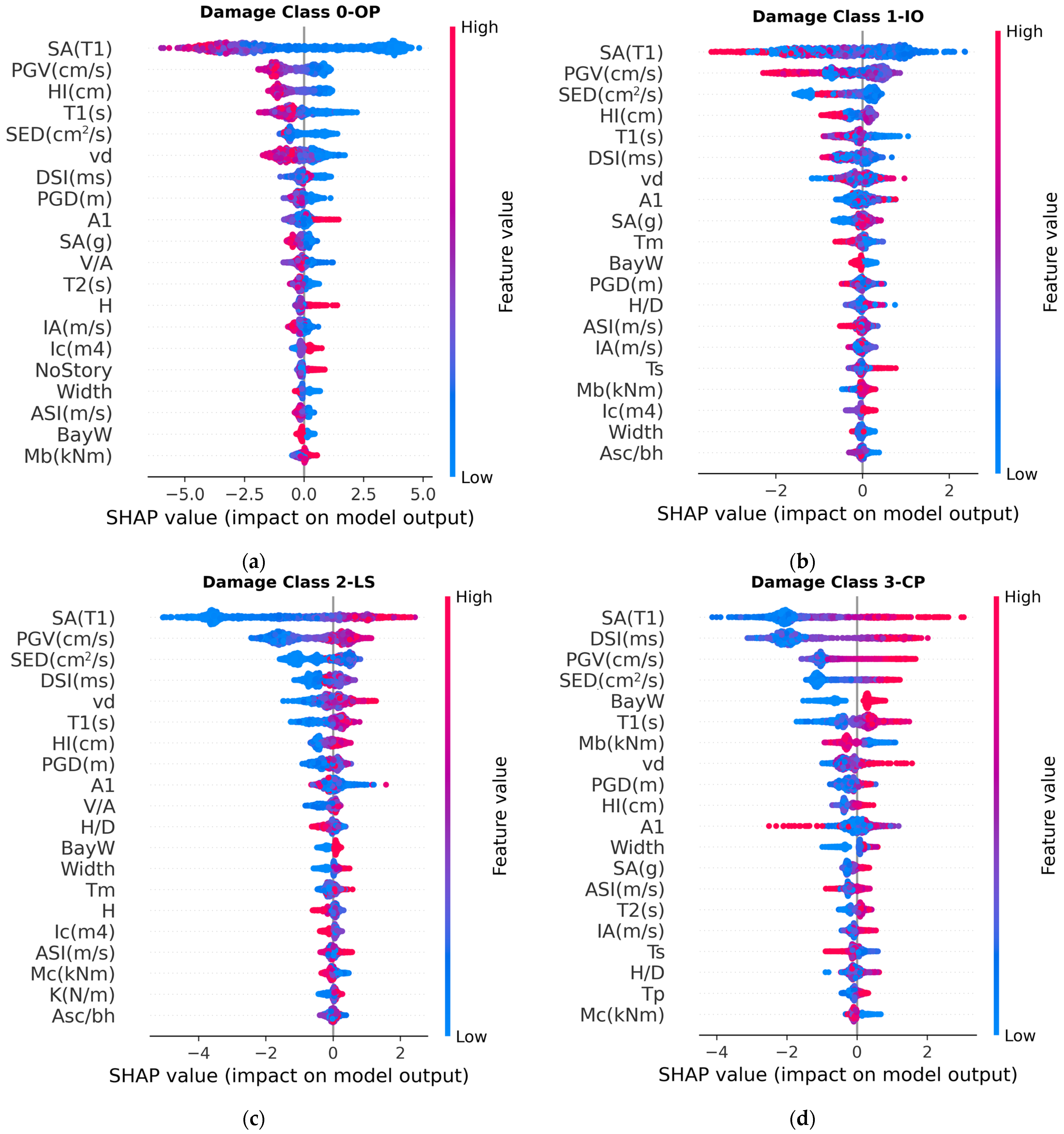
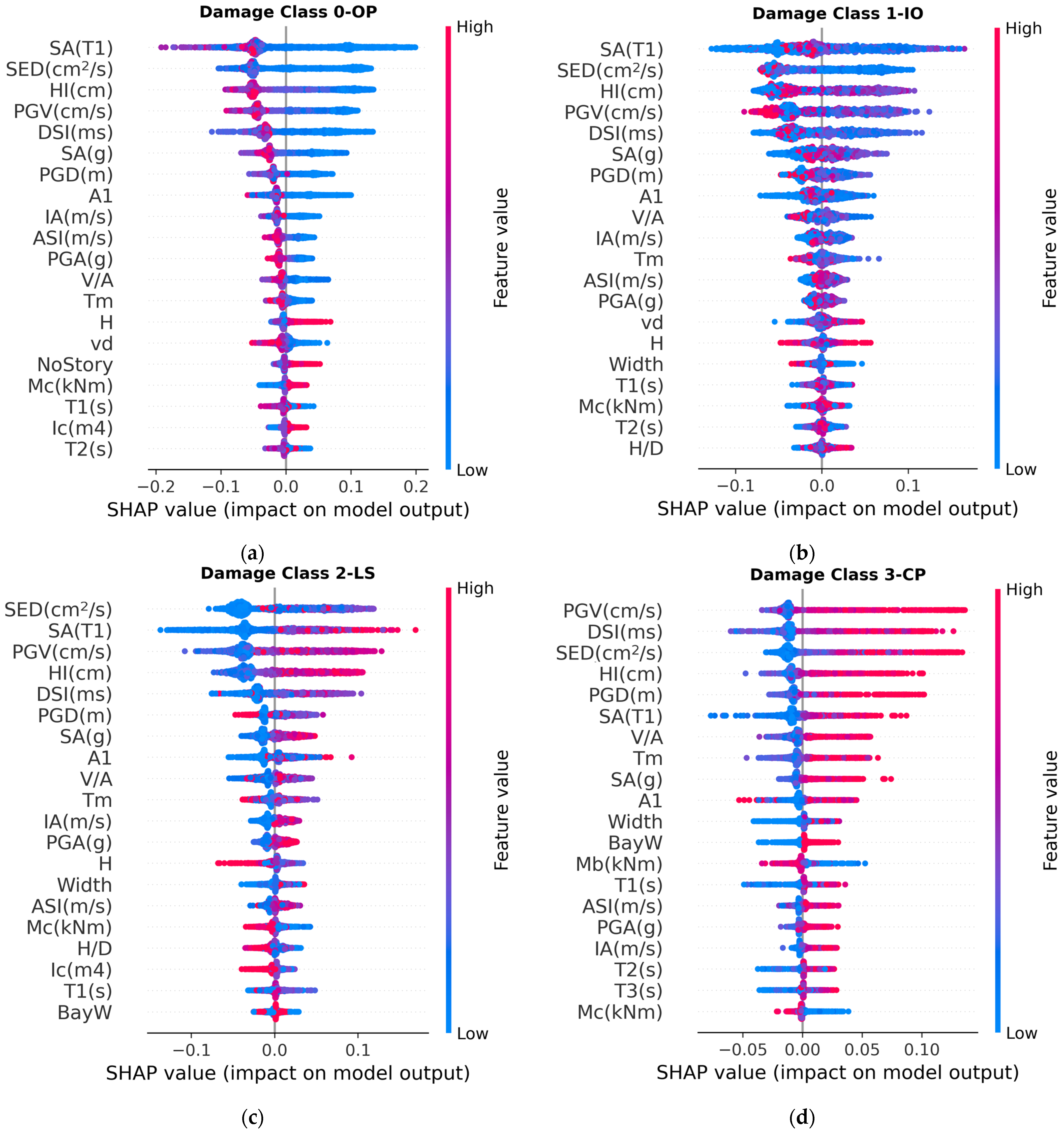
  • The feature importance study based on impurity-based feature importance and SHAP values revealed that earthquake parameters, such as velocity-related parameters and spectral acceleration in the fundamental period, generally have large impacts on the outputs. Moreover, the geometry of buildings, maximum axial load level, first-mode vibration period, and column properties were important structural parameters that affect the outputs. The results provide valuable insights for selecting input features for future ML model development.
  • ML models with optimized numbers of input features for preliminary damage classification were developed for practical applications. The studies indicated that most of the ML models could reach adequate accuracy even though the number of input features decreased. In this case, XGBoost performed the best among the other ML models under consideration. The performance of AdaBoost and RF was slightly lower than that of XGBoost. On the other hand, the performance of ANN models was satisfactory but lower than that of most of the ensemble methods.
  • The ML models developed in this study are suitable for estimating the damage class of RC frames that are designed without considering seismic effects, and as such, they are suitable for buildings located in non-seismically active regions. In addition, the models were trained using far-field earthquakes. Under the conditions of near-field earthquakes, models may fail to account for the pulse-like characteristics of seismic waves.

Future Work

The dataset can be further increased to capture buildings and structures with various conditions. For example, structural eccentricity, shear wall ratios, etc., could be considered. On the other hand, regression models for the prediction of structural responses, such as MIDR, could be developed. Possible improvements in ML model development, such as using the entire earthquake history instead of earthquake parameters, should be investigated. Moreover, the architecture of the neural network models can be further enhanced by introducing other techniques, such as convolutional layers, transformer layers, or transfer learning. Instead of using earthquake parameters, earthquake histories could be taken as inputs of ML models. In this case, CNN is helpful to extract important features from earthquake histories before passing to the dense layers. On the other hand, CNN and transformers can be adopted to process tabular data by finding out the possible relationships between input features so as to improve the accuracy of the ANN models.

Funding

This study was supported by the grant from the Research Grants Council of the Hong Kong Special Administrative Region, China (Project No. UGC/FDS25/E05/21).

Data Availability Statement

The data will be made available upon request.

Acknowledgments

This article is a revised and expanded version of a paper entitled “Damage Class Prediction using Machine Learning Algorithm”, which was presented at ASEM23, Seoul National University, Seoul, Korea [48].

Conflicts of Interest

The author declares no conflicts of interest.

Abbreviations

The following abbreviations are used in this manuscript:
ANNArtificial Neural Network
ASIAcceleration Spectrum Intensity
AdaBoostAdaptive Boosting
CNNConvolutional Neural Network
DTDecision Tree
DSIDisplacement Spectrum Intensity
ETExtra Tree
FRPFiber-Reinforced Polymer
GBDTGradient Boosting Decision Tree
GFRPGlass Fiber-Reinforced Polymer
IDAIncremental Dynamic Analysis
IMIntensity Measure
KNNK-Nearest Neighbor
LightGBMLight Gradient Boosting Machine
LRLogistic Regression
MIDRMaximum Inter-story Drift Ratio
MLMachine Learning
NBNaïve Bayes
NLTHANon-Linear Time–History Analysis
PGAPeak Ground Acceleration
PGDPeak Ground Displacement
PGVPeak Ground Velocity
RFRandom Forest
ROCReceiver Operating Characteristic
SEDSpecific Energy Density
SHAPSHapley Additive exPlanations
SVMSupport Vector Machine
XGBoosteXtreme Gradient Boosting

Appendix A

The list of earthquake records used in the incremental dynamic analyses is presented in Table A1. The earthquake records used in this study were taken from ATC-63 Ground Motion Set [71]. The far-field ground motion set was utilized. Earthquakes from different events were considered to minimize the possibility that the results are dominated by a single event.
Table A1. List of earthquake records.
IndexName
A1940 Elcentro
B1995 Kobe
C1999 Chichi
D1994 Northridge
E1980 Campano Lucano
F1979 Imperial Valley
G1989 Loma Prieta
H1999 Duzce
I1999 Kocaeli
J1971 San Fernando
K1976 Friuli
L1999 Hector Mine
M1992 Landers
N1990 Manjil
O1987 Superstition Hills
P1992 Cape Mendocino

Appendix B

The ranges of hyper-parameters for basic models and ensemble models adopted in optuna are presented in Table A2. The number of trails was taken as 100.
Table A2. Ranges of hyper-parameters used in optuna.
ModelHyper-Parameter
Logistic regression (LR)‘C’: [0.1, 30.0]
‘solver’: [‘newton-cg’, ‘lbfgs’, ‘liblinear’, ‘saga’]
Support vector machine (SVM)‘C’: [1, 50]
‘kernel’: [‘linear’, ‘poly’, ‘rbf’]
Decision tree (DT)‘criterion’: [‘gini’, ‘entropy’, ‘log_loss’]
‘max_depth’: [5, 50]
K-nearest neighbor (KNN)‘algorithm’: [‘auto’, ‘ball_tree’, ‘kd_tree’, ‘brute’]
‘n_neighbors’: [5, 20]
Bagging (SVM)‘n_estimators’: [10, 200]
Random forest (RF)‘n_estimators’: [100, 500]
Bagging (extra trees)‘n_estimators’: [100, 500]
Gradient boosting DT (GBDT)‘n_estimators’: [100, 500]
AdaBoost (ADA)‘n_estimators’: [50, 200]
XGBoost‘n_estimators’: [100, 500]
‘alpha’: [0.001, 1.0]
‘subsample’: [0.2, 1.0]
LightGBM‘num_leaves’: [10, 200]
‘max_depth’: [10, 200]

References

  1. Nazari, Y.R.; Saatcioglu, M. Seismic vulnerability assessment of concrete wall buildings through fragility analysis. J. Build. Eng. 2017, 12, 202–209. [Google Scholar] [CrossRef]
  2. Saleemuddin, M.Z.M.; Sangle, K.K. Seismic damage assessment of reinforced concrete structure using non-linear static analysis. KSCE J. Civ. Eng. 2017, 21, 1319–1330. [Google Scholar] [CrossRef]
  3. Bektas, N.; Kegyes-Brassai, O. Enhancing seismic assessment and risk management of buildings: A neural network-based rapid visual screening method development. Eng. Struct. 2024, 304, 117606. [Google Scholar] [CrossRef]
  4. EN1998-1:2004; Eurocode 8: Design of Structures for Earthquake Resistance. European Committee for Standardization: Brussels, Belgium, 2004.
  5. FEMA356; Prestandard and Commentary for the Seismic Rehabilitation of Buildings. American Society of Civil Engineers: Reston, VA, USA, 2000.
  6. ASCE41-17; Seismic Evaluation and Retrofit of Existing Buildings. American Society of Civil Engineers: Reston, VA, USA, 2017.
  7. Kuria, K.K.; Kegyes-Brassai, O.K. Pushover analysis in seismic engineering: A detailed chronology and review of techniques for structural assessment. Appl. Sci. 2024, 14, 151. [Google Scholar] [CrossRef]
  8. Chopra, A.K.; Goel, R.K. A modal pushover analysis procedure for estimating seismic demands for buildings. Earthq. Eng. Struct. Dyn. 2001, 31, 561–582. [Google Scholar] [CrossRef]
  9. Kreslin, M.; Fajfar, P. The extended N2 method considering higher mode effects in both plan and elevation. Bull. Earthq. Eng. 2012, 10, 695–715. [Google Scholar] [CrossRef]
  10. Xu, W.X.; Zhao, Y.S.; Yang, W.S.; Yu, D.H.; Zhao, Y.D. Seismic fragility analysis of RC frame structures based on IDA analysis and machine learning. Structures 2024, 65, 106774. [Google Scholar] [CrossRef]
  11. Vamvatsikos, D.; Cornell, C.A. Incremental dynamic analysis. Earthq. Eng. Struct. Dyn. 2002, 31, 491–514. [Google Scholar] [CrossRef]
  12. Cardone, D.; Rossino, M.; Cesualdi, G. Estimating fragility curves of pre-70 RC frame buildings considering different performance limit states. Soil Dyn. Earthq. Eng. 2018, 115, 868–881. [Google Scholar] [CrossRef]
  13. Pandikkadavath, M.S.; Shaijal, K.M.; Mangalathu, S.; Davis, R. Seismic robustness assessment of steel moment resisting frames employing material uncertainty incorporated incremental dynamic analysis. J. Constr. Steel Res. 2022, 191, 107200. [Google Scholar] [CrossRef]
  14. Peng, W.J.; Li, Z.A.; Tao, M.X. Evaluation of performance and storey drift ratio limits of high-rise structural systems with separated gravity and lateral load resisting systems using time history analysis and incremental dynamic analysis. Structures 2023, 56, 104961. [Google Scholar] [CrossRef]
  15. Pizarro, P.N.; Massone, L.M.; Rojas, F.R.; Ruiz, R.O. Use of convolutional networks in the conceptual structural design of shear wall buildings layout. Eng. Struct. 2021, 239, 1–19. [Google Scholar] [CrossRef]
  16. di Stefano, A.G.; Ruta, M.; Masera, G.; Hoque, S. Leveraging machine learning to forecast neighborhood energy use in early design stages: A preliminary application. Buildings 2024, 14, 3866. [Google Scholar] [CrossRef]
  17. Hosamo, H.; Mazzetto, S. Performance evaluation of machine learning models for predicting energy consumption and occupant dissatisfaction in buildings. Buildings 2025, 15, 39. [Google Scholar] [CrossRef]
  18. Salehi, H.; Burgueno, R. Emerging artificial intelligence methods in structural engineering. Eng. Struct. 2018, 171, 170–189. [Google Scholar] [CrossRef]
  19. Xie, Y.; Sichani, M.E.; Padgett, J.E.; DesRoches, R. The promise of implementing machine learning in earthquake engineering: A state-of-the-art review. Earthq. Spectra 2020, 36, 1769–1801. [Google Scholar] [CrossRef]
  20. Sun, H.; Burton, H.V.; Huang, H. Machine learning applications for building structural design and performance assessment: State-of-the-art review. J. Build. Eng. 2021, 33, 101816. [Google Scholar] [CrossRef]
  21. Pan, Y.; Zhang, L. Roles of artificial intelligence in construction engineering and management: A critical review and future trends. Autom. Constr. 2021, 122, 103517. [Google Scholar] [CrossRef]
  22. Thai, H.T. Machine learning for structural engineering: A state-of-the-art review. Structures 2022, 38, 448–491. [Google Scholar] [CrossRef]
  23. Raschka, S.; Mirjalili, V. Python Machine Learning, Machine Learning and Deep Learning with Python, Scikit-Learn and TensorFlow 2, 3rd ed.; Packt Publishing Ltd.: Birmingham, UK, 2019. [Google Scholar]
  24. Giovanis, D.G.; Fragiadakis, M.; Papadopoulos, V. Epistemic uncertainty assessment using incremental dynamic analysis and neural networks. Bull. Earthq. Eng. 2015, 14, 529–547. [Google Scholar] [CrossRef]
  25. Morfidis, K.; Kostinakis, K. Approaches to the rapid seismic damage prediction of r/c buildings using artificial neural networks. Eng. Struct. 2018, 165, 120–141. [Google Scholar] [CrossRef]
  26. Dabiri, H.; Faramarzi, A.; Dall’Asta, A.; Tondi, E.; Fabio, M. A machine learning-based analysis for predicting fragility curve parameters of buildings. J. Build. Eng. 2022, 62, 105367. [Google Scholar] [CrossRef]
  27. Demertzis, K.; Kostinakis, K.; Morfidis, K.; Iliadis, L. An interpretable machine learning method for the prediction of R/C buildings’ seismic response. J. Build. Eng. 2023, 63, 105493. [Google Scholar] [CrossRef]
  28. Shahnazaryan, D.; O’Reilly, G.J. Next-generation non-linear and collapse prediction models for short-to-long-period systems via machine learning methods. Eng. Struct. 2024, 306, 117801. [Google Scholar] [CrossRef]
  29. Demir, A.; Sahin, E.K.; Demir, S. Advanced tree-based machine learning methods for predicting the seismic response of regular and irregular RC frames. Structures 2024, 64, 106524. [Google Scholar] [CrossRef]
  30. Işık, M.F.; Avcil, F.; Harirchian, E.; Bülbül, M.A.; Hadzima-Nyarko, M.; Işık, E.; İzol, R.; Radu, D. A hybrid artificial neural network—Particle swarm optimization algorithm model for the determination of target displacements in mid-rise regular reinforced-concrete buildings. Sustainability 2023, 15, 9715. [Google Scholar] [CrossRef]
  31. Payán-Serrano, O.; Bojórquez, E.; Carrillo, J.; Bojórquez, J.; Leyva, H.; Rodríguez-Castellanos, A.; Carvajal, J.; Torres, J. Seismic performance prediction of RC, BRB and SDOF structures using deep learning and the intensity measure INp. AI 2024, 5, 1496–1516. [Google Scholar] [CrossRef]
  32. Hwang, S.H.; Mangalathu, S.; Shin, J.; Jeon, J.S. Machine learning-based approaches for seismic demand and collapse of ductile reinforced concrete building frame. J. Build. Eng. 2021, 34, 101905. [Google Scholar] [CrossRef]
  33. Bhatta, S.; Dang, J. Seismic damage prediction of RC buildings using machine learning. Earthq. Eng. Struct. Dyn. 2023, 52, 3504–3527. [Google Scholar] [CrossRef]
  34. Mahmoudi, H.; Bitaraf, M.; Salkhordeh, M.; Soroushian, S. A rapid machine learning-based damage detection algorithm for identifying the extent of damage in concrete shear-wall buildings. Structures 2023, 47, 482–499. [Google Scholar] [CrossRef]
  35. Zhang, H.Y.; Cheng, X.W.; Li, Y.; He, D.J.; Du, X.L. Rapid seismic damage state assessment of RC frames using machine learning methods. J. Build. Eng. 2023, 65, 105797. [Google Scholar] [CrossRef]
  36. Kostinakis, K.; Morfidis, K.; Demertzis, K.; Iliadis, L. Classification of buildings’ potential for seismic damage using a machine learning model with auto hyperparameter tuning. Eng. Struct. 2023, 290, 116359. [Google Scholar] [CrossRef]
  37. Wei, Z.; Wang, X.; Fan, B.; Shahzad, M.M. A stacking ensemble-based multi-channel CNN strategy for high-accuracy damage assessment in mega-sub controlled structures. Buildings 2025, 15, 1775. [Google Scholar] [CrossRef]
  38. Imam, M.H.; Mohiuddin, M.; Shuman, N.M.; Oyshi, T.I.; Debnath, B.; Liham, M.I.M.H. Prediction of seismic performance of steel frame structures: A machine learning approach. Structures 2024, 69, 107547. [Google Scholar] [CrossRef]
  39. Asgarkhani, N.; Kazemi, F.; Jakubczyk-Galczynska, A.; Mohebi, B.; Jankowski, R. Seismic response and performance prediction of steel buckling-restrained braced frames using machine-learning methods. Eng. Appl. Artif. Intell. 2024, 128, 107388. [Google Scholar] [CrossRef]
  40. Kazemi, P.; Ghisi, A.; Mariani, S. Classification of the structural behavior of tall buildings with a diagrid structure: A machine learning-based approach. Algorithms 2022, 15, 349. [Google Scholar] [CrossRef]
  41. To, Q.B.; Lee, K.; Cuong, N.H.; Shin, J. Development of machine learning based seismic retrofit scheme for AFRP retrofitted RC column. Structures 2024, 69, 107279. [Google Scholar] [CrossRef]
  42. Babiker, A.; Abbas, Y.M.; Khan, M.I.; Ismail, F.I. From robust deep-learning regression to refined design formulas for punching shear strength of internal GFRP-reinforced flat slab-column connections. Eng. Struct. 2025, 326, 119534. [Google Scholar] [CrossRef]
  43. Wu, C.; Ma, G.; Zhu, D.; Qu, H.; Zhuang, H. Seismic retrofitting of GFRP-reinforced concrete columns using precast UHPC plates. Soil Dyn. Earthq. Eng. 2024, 187, 109024. [Google Scholar] [CrossRef]
  44. Junda, E.; Malaga-Chuquitaype, C.; Chawgien, K. Interpretable machine learning models for the estimation of seismic drifts in CLT buildings. J. Build. Eng. 2023, 70, 106365. [Google Scholar] [CrossRef]
  45. Zong, C.; Zhai, J.; Sun, X.; Liu, X.; Cheng, X.; Wang, S. Analysis of seismic responses and vibration serviceability in a high-rise timber-concrete hybrid building. Buildings 2024, 14, 2614. [Google Scholar] [CrossRef]
  46. Buildings Department. The Hong Kong Code of Practice for Structural Use of Concrete 2013; Hong Kong Special Administrative Region (HKSAR): Hong Kong, China, 2020. [Google Scholar]
  47. Luk, S.H.; Wong, H.F. Fragility curves for buildings in Hong Kong. In Proceedings of the 2019 World Congress on Advances in Structural Engineering and Mechanics (ASEM19), Jeju Island, Republic of Korea, 17–21 September 2019. [Google Scholar]
  48. Luk, S.H. Damage Class Prediction using Machine Learning Algorithm. In Proceedings of the 2023 World Congress on Advances in Structural Engineering and Mechanics (ASEM23), Seoul National University, Seoul, Republic of Korea, 16–18 August 2023. [Google Scholar]
  49. Park, Y.J.; Ang, A.H. Mechanistic seismic model for reinforced concrete. J. Struct. Eng. 1985, 111, 722–739. [Google Scholar] [CrossRef]
  50. Kappos, A.J. Seismic damage indices for RC buildings. Prog. Struct. Eng. Mater. 1997, 1, 78–87. [Google Scholar] [CrossRef]
  51. Banon, H.; Biggs, J.M.; Irvine, H.M. Seismic damage in reinforced concrete frames. J. Struct. Eng. 1981, 107, 1713–1729. [Google Scholar] [CrossRef]
  52. Di Pasquale, E.; Cakmak, A.S. Identification of the Serviceability Limit State and Detection of Seismic Structural Damage; Technical Report NCEER-87-0022; State University of New York: Buffalo, NY, USA, 1988. [Google Scholar]
  53. FEMA. Hazus Earthquake Model Technical Manual; Hazus 5.1; Federal Emergency Management Agency: Washington, DC, USA, 2022.
  54. Pedregosa, F.; Varoquaux, G.; Gramfort, A.; Michel, V.; Thirion, B.; Grisel, O.; Blondel, M.; Prettenhofer, P.; Weiss, R.; Dubourg, V.; et al. Scikit-learn: Machine learning in Python. J. Mach. Learn. Res. 2011, 12, 2825–2830. [Google Scholar] [CrossRef]
  55. Akiba, T.; Sano, S.; Yanase, T.; Ohta, T.; Koyama, M. A next-generation hyperparameter optimization framework. In Proceedings of the 25th SIGKDD Conference on Knowledge Discovery & Data Mining, Anchorage, AK, USA, 4–8 August 2019. [Google Scholar] [CrossRef]
  56. Hosmer, D.W.; Lemeshow, S. Applied Logistic Regression, 2nd ed.; John Wiley: Hoboken, NJ, USA, 2000. [Google Scholar]
  57. Cortes, C.; Vapnik, V. Support-vector networks. Mach. Learn. 1995, 20, 273–297. [Google Scholar] [CrossRef]
  58. Goldberger, J.; Roweis, S.; Hinton, G.; Salakhutdinov, R. Neighborhood components analysis. In Advances in Neural Information Processing Systems 17; MIT Press: Cambridge, MA, USA, 2005; pp. 513–520. [Google Scholar]
  59. Breiman, L.; Friedman, J.; Olshen, R.A.; Stone, C.J. Classification and Regression Trees, 1st ed.; Chapman and Hall/CRC: New York, NY, USA, 1984. [Google Scholar] [CrossRef]
  60. Wolpert, D.H. Stacked generalization. Neural Netw. 1992, 5, 241–259. [Google Scholar] [CrossRef]
  61. Ho, T.K. Random decision forests. In Proceedings of the 3rd International Conference on Document Analysis and Recognition, Montreal, QC, Canada, 14–16 August 1995. [Google Scholar] [CrossRef]
  62. Freund, Y.; Schapiren, R.E. A decision-theoretic generalization of on-line learning and an application to boosting. J. Comput. Syst. Sci. 1997, 55, 119–139. [Google Scholar] [CrossRef]
  63. Friedman, J.H. Greedy function approximation: A gradient boosting machine. Ann. Stat. 2001, 29, 1189–1232. [Google Scholar] [CrossRef]
  64. Chen, T.; Guestrin, C. XGBoost: A scalable tree boosting system. In Proceedings of the 22nd ACM SIGKDD International Conference on Knowledge Discovery and Data Mining, Association for Computing Machinery, San Francisco, CA, USA, 13–17 August 2016. [Google Scholar] [CrossRef]
  65. Ke, G.; Meng, Q.; Finley, T.; Wang, T.; Chen, W.; Ma, W.; Ye, Q.; Liu, T.Y. LightGBM: A highly efficient gradient boosting decision tree. Advances in Neural Information Processing Systems. In Proceedings of the 31st Conference on Neural Information Processing Systems (NIPS 2017), Red Hook, NY, USA, 4–9 December 2017. [Google Scholar]
  66. Atienza, R. Advanced Deep Learning with TensorFlow 2 and Keras, 2nd ed.; Packt Publishing Ltd.: Birmingham, UK, 2020. [Google Scholar]
  67. Rumelhart, D.; Hinton, G.; Williams, R. Learning representations by back-propagating errors. Nature 1986, 323, 533–536. [Google Scholar] [CrossRef]
  68. Emami, S.; Martínez-Muñoz, G. Sequential training of neural networks with gradient boosting. IEEE Access 2023, 11, 42738–42750. [Google Scholar] [CrossRef]
  69. Oh, B.K.; Glisic, B.; Park, S.W.; Park, H.S. Neural network-based seismic response prediction model for building structures using artificial earthquakes. J. Sound Vib. 2020, 468, 115109. [Google Scholar] [CrossRef]
  70. Stafford Smith, B.; Coull, A. Tall Building Structures: Analysis and Design; John Wiley & Sons, Inc.: Hoboken, NJ, USA, 1991. [Google Scholar]
  71. FEMA P-695. Quantification of Building Seismic Performance Factors; Federal Emergency Management Agency: Washington, DC, USA, 2009.
Figure 1. Flow chart of the methodology.
Buildings 15 02395 g001
Figure 2. Sample of building models.
Buildings 15 02395 g002
Figure 3. Basic machine learning algorithms.
Buildings 15 02395 g003
Figure 4. Ensemble methods.
Buildings 15 02395 g004
Figure 5. General neural network architecture.
Buildings 15 02395 g005
Figure 6. Architecture of a stacking ANN.
Buildings 15 02395 g006
Figure 7. Confusion matrices for (a) support vector machine, (b) random forest, (c) XGBoost, and (d) ANN with three hidden layers (128 units).
Buildings 15 02395 g007aBuildings 15 02395 g007b
Figure 8. ROC curves for (a) SVM, (b) random forest, (c) XGBoost, and (d) ANN.
Buildings 15 02395 g008aBuildings 15 02395 g008b
Figure 9. Feature importance: (a) XGBoost and (b) random forest.
Buildings 15 02395 g009
Figure 10. SHAP values for XGBoost: (a) damage class 0; (b) damage class 1; (c) damage class 2; and (d) damage class 3.
Buildings 15 02395 g010
Figure 11. SHAP values for RF: (a) damage class 0; (b) damage class 1; (c) damage class 2; and (d) damage class 3.
Buildings 15 02395 g011
Table 2. Examples of damage indices.
NameDefinitionProposed by
Flexural damage ratio (stiffness-based) D I = M u ϕ m M m ϕ u Banon et al. [51]
Park and Ang damage index (combined) D = δ m δ u + β F y δ u d E Park and Ang [49]
Period-based damage D I = 1 T a T m DiPasquale and Cakmak [52]
Max. inter-story drift ratio M I D R = max u i + 1 u i h -
Table 3. Definition of damage levels (FEMA 356).
Damage Level/Label0123
Performance 1OPIOLSCP
MIDR<1.0%>1.0%>2.0%>4.0%
1 OP—operational performance; IO—immediate occupancy performance; LS—life safety performance; CP—collapse prevention performance.
Table 4. Summary of hyper-parameters for the ML models.
ML ModelHyper-Parameters
Logistic regression (LR)C = 25, solver = lbfgs
Support vector machine (SVM)C = 45, kernel = poly
Decision tree (DT)max_depth = 20, criterion = gini
K-nearest neighbor (KNN)n_neighbors = 10, weights = distance
Gaussian Naïve Bayes (NB)-
Bagging (SVM)n_estimators = 100
Random forest (RF)n_estimators = 300, criterion = log_loss
Bagging (extra trees)n_estimators = 210, criterion = log_loss
Gradient boosting DT (GBDT)n_estimators = 240, learning_rate = 0.5
AdaBoost (ADA)estimator = DT (max_depth = 10), n_estimators = 180, learning_rate = 1.0
XGBoostbooster = gbtree, eta = 0.1, n_estimators = 450, lambda = 1.0, alpha = 0.01, subsample = 0.7
LightGBMmax_depth = 100, num_leaves = 200, num_iterations = 200
Voting (basic)estimator = (LR, SVM, DT, KNN)
Voting (ensemble)estimator = (RF, XGB, GBDT)
Stacking (basic)estimator = (LR, SVM, DT, KNN), final estimator = LR (C = 20)
Stacking (ensemble)estimator = (RF, XGB, GBDT), final estimator = LR (C = 20)
ANN-11 hidden layer: 128
ANN-21 hidden layer: 256
ANN-32 hidden layers: 128, 128
ANN-42 hidden layers: 256, 256
ANN-53 hidden layers: 128, 128, 128
ANN-63 hidden layers: 256, 256, 256
Stacking ANN5 ANN models (2 hidden layers: 128, 128), meta-learner = LR (C = 3.0)
Boosting ANNN = 25, eta = 0.2, weak learner = ANN (2 hidden layers: 128, 128)
Table 5. Definitions of earthquake parameters.
Earthquake ParameterNameDefinitionMeanStandard Deviation (S.D.)
PGA (g)Peak ground acceleration m a x u ¨ ( t ) 0.550.29
PGV (cm/s)Peak ground velocity m a x u ˙ ( t ) 64.3144.33
PGD (m)Peak ground displacement m a x u ( t ) 0.370.34
Sa1Spectrum acceleration at T = 1.0 s S a ( T = 1.0   s , ξ = 5 % ) 0.640.40
Sa(T1)Spectrum acceleration at T1 S a ( T 1 , ξ = 5 % ) 0.270.31
ASI (m/s)Acceleration spectrum intensity A S I = 0.1 0.5 S a ( ξ = 5 % ) d T 0.470.25
HI (cm)Housner intensity H I = 0.1 2.5 S v ( ξ = 5 % ) d T 203.18127.49
DSI (m-s)Displacement spectrum intensity D S I = 5.0 2.0 S d ( ξ = 5 % ) d T 1.291.29
V/ARatio between PGV and PGA P G V / P G A 0.120.05
Ia (m/s)Arias intensity I a = π 2 g 0 t u ˙ ( t ) 2 d t 4.984.76
Tm (s)Mean period T m = i N C i 2 × 1 f i i N C i 2
where C i is the Fourier amplitude at frequency f i
0.670.29
Tp (s)Predominant periodTime to reach max S a 0.300.17
Ts (s)Significant durationTime between 5% and 95% of I a 14.917.47
SED (cm2/s)Specific energy density S E D = 0 t u ˙ ( t ) 2 d t 9856.8116,053.95
A1 [69]Resonance areaFFT area of a seismic wave at a frequency range near the natural frequency of the building112.73158.19
Table 6. Definitions of structural parameters.
NameMeanStandard Deviation (S.D.)
Number of stories10.15.38
Height, H (m)37.720.39
Number of bays3.30.57
Bay width (m)5.60.49
Width of building, W (m)18.33.86
Aspect ratio, H/W2.01.23
Max axial load ratio, vd = N/fcuAc1.110.12
Moment of inertia of beam, Ib = bh3/12 (m4)2.83 × 10−32.44 × 10−3
Moment of inertia of column, Ic = bh3/12 (m4)2.59 × 10−34.97 × 10−3
Moment resistance of beam, Mb (kNm)426.8488.2
Moment resistance of column, Mc (kNm)265.7529.01
First-mode period, T1 (s)2.651.23
Second-mode period, T2 (s)0.860.41
Third-mode period, T3 (s)0.500.24
Fourth-mode period, T4 (s)0.350.17
Steel ratio of beam, ρ s b = Asb/bh1.47%0.35%
Steel ratio of column, ρ s c = Asc/bh2.91%0.65%
Story stiffness, K (N/m) [70]21,811.123,277.4
Table 7. Performance of ML models for damage classification.
ML ModelAccuracyPrecisionRecallF1-ScoreROC AUC Score
1. Basic models
Logistic regression (LR)0.8010.7920.7710.7800.951
Support vector machine (SVM)0.8650.8600.8470.8530.976
Decision tree (DT)0.8200.8040.8080.8060.873
K-nearest neighbor (KNN)0.8040.8100.7820.7940.954
Gaussian Naïve Bayes0.6970.6730.6770.6730.904
2. Ensemble models
Bagging (SVM)0.8680.8810.8360.8530.978
Random forest (RF)0.8800.8760.8630.8690.981
Bagging (Extra trees, ET)0.8740.8680.8560.8610.980
Gradient Boosting DT (GBDT)0.8770.8690.8570.8620.978
AdaBoost (AdaBoost)0.8860.8860.8650.8740.982
XGBoost (XGBoost)0.8910.8850.8770.8800.984
LightGBM0.8810.8760.8650.8700.980
Voting (LR, KNN, DT, SVM)0.8610.8620.8420.8510.976
Voting (RF, XGB, ADA)0.8830.8780.8680.8720.982
Stacking (KNN, DT, SVM, LR)0.8620.8640.8410.8510.964
Stacking (RF, XGB, ADA)0.8880.8840.8710.8770.964
3. Artificial neural networks
ANN-1 (1 layer: 128)0.8660.8640.8490.8540.977
ANN-2 (1 layer: 256)0.8680.8660.8500.8560.979
ANN-3 (2 layers: 128, 128)0.8710.8670.8580.8610.980
ANN-4 (2 layers: 256, 256)0.8680.8610.8620.8600.979
ANN-5 (3 layers: 128, 128, 128)0.8720.8680.8620.8640.980
ANN-6 (3 layers: 256, 256, 256)0.8670.8570.8580.8560.978
Stacking ANN0.8820.8790.8690.8740.983
Gradient boosting ANN0.8850.8850.8690.8760.982
Table 8. Performance of the modified ML models.
ML ModelAccuracyPrecisionRecallF1-ScoreROC AUC Score
1. Basic model
Support vector machine (SVM)0.8660.8630.8400.8500.975
2. Ensemble models
Random forest (RF)0.8750.8660.8540.8590.980
Bagging (extra trees, ET)0.8680.8620.8480.8540.978
Gradient boosting DT (GBDT)0.8600.8480.8350.8410.971
AdaBoost (AdaBoost)0.8780.8750.8560.8640.980
XGBoost (XGBoost)0.8820.8740.8630.8680.982
LightGBM0.8730.8620.8520.8560.978
3. Artificial neural networks
ANN-1 (2 layers: 128, 128)0.8640.8550.8370.8440.976
ANN-2 (2 layers: 256, 256)0.8680.8590.8470.8520.977
ANN-3 (3 layers: 128, 128, 128)0.8640.8570.8430.8480.976
ANN-4 (3 layers: 256, 256, 256)0.8560.8410.8430.8410.976
Stacking ANN0.8700.8630.8480.8540.977
Gradient boosting ANN0.8730.8660.8520.8580.979
Disclaimer/Publisher’s Note: The statements, opinions and data contained in all publications are solely those of the individual author(s) and contributor(s) and not of MDPI and/or the editor(s). MDPI and/or the editor(s) disclaim responsibility for any injury to people or property resulting from any ideas, methods, instructions or products referred to in the content.

